1. INTRODUCTION
Recently, advances in the high-intensity laser technology has enabled researcher to explore new physics of laser–plasma interaction. The major issue of research in all laser–plasma applications, including laser-induced fusion (Deutsch et al., Reference Deutsch, Furukawa, Mima, Murakami and Nishihara1996; Reference Deutsch, Bret, Firpo, Gremillet, Lefebrave and Lifschitz2008; Canaud et al., Reference Canaud, Fortin, Garaude, Meyer and Philippe2004; Hora et al., Reference Hora and Hoffmann2008; Hong et al., Reference Hong, He, Wen, Du, Teng, Qing, Huang, Huang, Liu, Wang, Huang, Zhu, Ding and Peng2009; Stancalie, Reference Stancalie2009) and plasma-based accelerators (Tajima & Dawson, Reference Tajima and Dawson1979; Kruer, Reference Kruer1988; Baiwen et al., Reference Baiwen, Ishiguro, Škoric, Takamaru and Sato2004; Giulietti et al., Reference Giulietti, Galimberti, Giulietti, Gizzi, Labate and Tomassini2005; Karmakar & Pukhov, Reference Karmakar and Pukhov2007; Shi, Reference Shi2007; Liu et al., Reference Liu, Cheng, Qian, Ge, Zhang and Wang2009) is to improve the propagation characteristics of the laser beam so as to get efficient coupling in laser–plasma interaction (Nakamura et al., Reference Nakamura, Mima, Sakagami, Johzaki and Nagatomo2008; Hora & Hoffmann, Reference Hora and Hoffmann2008; Kulagin et al., Reference Kulagin, Cherepenin, Hur, Lee and Suk2008; Laska et al., Reference Laska, Jungwirth, Krasa, Krousky, Pfeifer, Rohlena, Velyhan, Ullschmied, GAmmino, Torrisi, Badziak, Parys, Rosinski, Ryc and Wolowski2008; Hong et al., Reference Hong, He, Wen, Du, Teng, Qing, Huang, Huang, Liu, Wang, Huang, Zhu, Ding and Peng2009; Kline et al., Reference Kline, Montgomery, Rousseaux, Baton, Tassin, Hardin, Flippo, Johnson, Shimada, Yin, Albright, Rose and Amiranoff2009; Malekynia et al., Reference Malekynia, Ghoranneviss, Hora and Miley2009; Niknam et al., Reference Niknam, Rastbood, Bafandeh and Khorashadizadeh2014). The propagation of laser beam in plasma can lead to various parametric instabilities such as stimulated Raman (Purohit et al., Reference Purohit, Sharma and Sharma2012; Verma et al., Reference Verma, Sajal, Varshney, Kumar and Sharma2014) and Brillouin scattering (Gao et al., Reference Gao, Lu, Wang, He and Hasi2010; Sharma et al., Reference Sharma, Bhardwaj and Sharma2012) filamentation (Kaw et al., Reference Kaw, Schmidt and Wilcox1973; Sharma et al., Reference Sharma, Sharma and Chauhan2007; Deutsch et al., Reference Deutsch, Bret, Firpo, Gremillet, Lefebrave and Lifschitz2008; Bawaaneh et al., Reference Bawaaneh, Assayed, Said and Al-Awfi2014) and self-focusing of laser beam, two plasmon instability, and harmonic generation. The filamentation of laser beam during its propagation in the plasma is the fundamental issue in the context of laser–plasma coupling (Kaw et al., Reference Kaw, Schmidt and Wilcox1973; Sharma & Sharma, Reference Sharma and Sharma2009). One of the major difficulties in understanding the features of the experimental results is that most of the theories of laser–plasma interactions are based on the assumption of a uniform laser pump. This is contrary to almost all the experimental situations where laser beams of finite transverse size having nonuniform intensity distribution along their wave front are used. Such beams may modify the background plasma density and suffer filamentation. The origin of filamentation instability may also be attributed to small scale density perturbations resulting from quasi neutrality or small-scale intensity spikes associated with the main beam (Kothari & Kobayashi, Reference Kothari and Kobayashi1983). Thus, direct and indirect experimental evidence reveals that an apparently smooth looking laser beam has intensity spikes that may lead to optical distortion in nonlinear media.
Laser propagation in underdense plasma is characterized by several time scales and demonstrated for specific intensities. In many situations the laser can create different type of nonlinearities at different time scales according to the inequalities (a) τ<τpe or (b) τpe<τ<τpi; hence one can have different time regimes. Here τ is the laser pulse duration,τpi is the ion plasma period, and τpe is the electron plasma period. In case of (a) τ<τpe the relativistic nonlinearity is setup. This nonlinearity is setup almost instantaneously and electrons acquire relativistic quiver velocities within a few optical periods; therefore, they will be modeled as a relativistic fluid. The massive ions will form a cold nonrelativistic fluid. The relation τpi≫τpe shows that the electron motion is adiabatic with respect to the ions; therefore, the multiple scales analysis of the electron fluid equations can be generalized by simply allowing for a nonzero ion velocity. In case of (b) relativistic and ponderomotive nonlinearities are operative. In this case, electrons are expelled from the channel due to electron ponderomotive force but ions are not expelled due to their inertia. When the laser propagates in the plasma the relativistic mass variation of the electrons is very important source of nonlinearity in the refractive index (Esarey et al., Reference Esarey, Ting and Sprangle1988; Osman et al., Reference Osman, Castillo and Hora1999). The relativistic dependence of electronic mass on the quiver speed of electrons in the field of the beams causes a modification in the plasma frequency ω p. In the relativistic regime of interaction, the relativistic dielectric constant of the plasma takes the form  ${\rm \varepsilon} = 1 - {\rm \omega} _{\rm p}^2 /{\rm \gamma} {\rm \omega} _0^2, $ where γ = (1+α2/2)1/2, α = eE/m 0cωp, E is the electric field of the laser pulse. In this case, the uneven variation in γ along the wave front of the laser pulse causes the same effect as the ponderomotive force does in the nonrelativistic case. It is the change of the plasma frequency which is responsible for the attraction or repulsion of the beams. The theoretical work related to the relativistic nonlinearity was first started by C. E. Max and others (Max et al., Reference Max, Arons and Langdon1974; Sun et al., Reference Sun, Ott, Lee and Guzdar1987). Experiments are now being carried out, in which plasmas are irradiated by laser light with intensities >10l8 W/cm2. At such intensities, the free electrons in plasma undergo nonlinear motion due to their relativistic mass change as their quiver velocity approaches the speed of light. The experimental observation on relativistic self-focusing of a laser beam was reported by Borisov et al. (Reference Borisov, Borovskiy, Korobkin, Prokhorov, Shiryaev, Shi, Luk, McPherson, Solem, Boyer and Rhodes1992). Further, the study of laser–plasma interaction has been done with relativistic nonlinearity (Sprangle et al., Reference Sprangle, Ting and Tang1987; Shukla, Reference Shukla1990) and plasma wave excitation. Relativistic Langmuir wave generated by ultra-short pulse lasers is studied by Bingham et al. (Reference Bingham, de Angelis, Amin, Cairns and McNamara1992). The effect of relativistic self-focusing on plasma wave excitation by a hollow Gaussian beam has been investigated by Gupta et al. (Reference Gupta, Rafat and Sharma2011). Therefore, the study of laser–plasma interaction considering relativistic nonlinearity is significant.
When this relativistic motion is included, it is found that the equation for the light wave contains nonlinear terms, which contribute to the generation of harmonics of the incident light. Moreover, the highly nonlinear nature of the interaction of the laser pulse with plasmas can be studied with the harmonic emission (Meyer & Zhu, Reference Meyer and Zhu1987; Sprangle et al., Reference Sprangle, Tang and Esarey1987; Esarey et al., Reference Esarey, Ting, Sprangle, Umstadter and Liu1993; Mori et al., Reference Mori, Decker and Leemans1993; Zeng et al., Reference Zeng, Shen, Yu and Xu1996; Nuzzo et al., Reference Nuzzo, Zarcone, Ferrante and Basile2000) because it contains a significant feature of such interaction. Harmonics produced from short pulse laser-driven plasmas have several attractive characteristics; and it will allow for the direct study of relativistic motion of electrons and has received wider attention in the studies of oscillations of electrons in the intense laser fields. Relativistic laser guiding, harmonic generation, and wake field acceleration have been reported by Esarey et al. (Reference Esarey, Schroeder, Shadwick, Wurtele and Leemans2000). Esarey et al. (Reference Esarey, Ting, Sprangle, Umstadter and Liu1993) proposed a nonlinear cold fluid model valid for ultra-high intensities and used to analyze relativistic harmonic generation. Banerjee et al. (Reference Banerjee, Umstadter, Shah, Valenzuela and Maksimchuk2002) have studied experimentally the high-harmonic generation in relativistic laser–plasma interaction. Effect of self-focusing of Gaussian laser beam on the second-harmonic generation in relativistic plasma has been discussed by Walia and Singh (Reference Walia and Singh2014). Further, if the magnetic field occurs in the system externally or generated spontaneously the study of harmonic plays vital role in laser–plasma interaction. Besides, Harmonic generation offers an alternative source for short wavelength generation and an important tool for diagnostics of nonlinear media. Apart from that, many of the specific optical materials possess magnetic controllability and hence the study of harmonic generation is significant in various laboratory situations of dealing with those materials. Thus, we cannot overlook the study of harmonic generation with magnetic field as it is not ignorable in diagnostics. Harmonic generation in magneto plasma has been studied by various researchers. Resonant second-harmonic generation of a Gaussian electromagnetic beam in a collisional magneto plasma is studied by Kaur et al. (Reference Kaur, Sharma and Salih2009). Harmonic generation in multi-resonant plasma films has been studied by Vincenti et al. (Reference Vincenti, de Ceglia, Haus and Scalora2013). Direct observation of density-gradient effects in harmonic generation from plasma mirrors by Kahaly et al. (Reference Kahaly, Monchocé, Vincenti, Dzelzainis, Dromey, Zepf, Martin and Quéré2013). The plasma wave and the second-harmonic generation of intense laser beams due to relativistic effects have been studied by Salih et al. (Reference Salih, Sharma and Rafat2004). Phase matching for the third-harmonic generation in collisional magneto plasmas has been studied by Sodha et al. (Reference Sodha, Verma and Sharma2005). Generation of the plasma wave and the third-harmonic generation are studied by Gupta et al. (Reference Gupta, Sharma and Mahmoud2007); they have considered both the relativistic and ponderomotive nonlinearity in an unmagnetized plasma.
Further, there are several processes that can cause laser harmonics in plasmas. As far as the present work concerns, the plasma wave is considered and proposed as a source for producing the third-harmonics. Previously the phenomenon of plasma wave and harmonic generation has been investigated by several authors. The method accountable for plasma wave generation is usual  $\vec V \times \vec B$ force, where B is the static magnetic field and V is the drift velocity of plasma electrons in the laser field. Here, an electromagnetic wave propagating is considered in magneto plasma along the static magnetic field. Under the field of pump beam the energy of plasma electrons turn out to be relativistic and laser beam starts focusing and then again defocusing. Moreover, the focusing of small intensity spikes in the profile of the pump laser breaks it into multiple filamentary structures. These high-intensity filaments turn into the source of plasma wave generation at double of laser frequency. The interaction of this plasma wave with the laser beam leads to the generation of the third-harmonics in the plasma. The variation in the intensity of the magnetic field alters the dynamics of plasma electrons and hence the electron density gradient gets modified. This leads to change in the power of the plasma wave and hence harmonics.
Additionally, it is important to mention that most of the above cited research on harmonic generation deals with the propagation and transmission of laser beams in the paraxial approximation because in most cases the divergence angles of the investigated laser beams are very small, and the beam widths of the investigated laser beams are far greater than the wavelength. Hence, paraxial wave equation provides a precise explanation for wave beams adjacent to the axis if the beam width remains larger than the radiation wavelength λ during the transmission. Nevertheless, in particular investigational circumstances, it is essential to go beyond the paraxial calculation such as certain semiconductor injection lasers, solid-state lasers, generate wide-angle beams for which the paraxial estimate is not appropriate and certain improvements are required. Thus, in the present work we incorporate the off-axial rays also in the analysis.
Further, the present work is inspired by the work done by Gupta et al. (Reference Gupta, Sharma and Mahmoud2007) and Sodha et al. (Reference Sodha, Verma and Sharma2005). They have studied the third-harmonic generation in non-magneto plasma and magneto plasma, respectively. Gupta et al. (Reference Gupta, Sharma and Mahmoud2007) considered both relativistic and ponderomotive nonlinearities simultaneously with paraxial approximation. Salih et al. (Reference Salih, Sharma and Rafat2004) has investigated the second-harmonics with relativistic effects with paraxial approximation. So far, there are no attempts to study the third-harmonic generation in magneto plasma considering extended paraxial approximation with relativistic nonlinearity. Therefore in the present work, the study of the third-harmonic generation has been done considering relativistic nonlinearity with extended paraxial approximation. The paper is organized as follows. In Section 2, generation of electrostatic wave has been discussed. We have also derived the expression for the power of plasma wave by considering modified paraxial approximation when only relativistic nonlinearity is operative. In Section 3, we have derived the dynamical equation governing the power of third-harmonic generation and equation for the beam width parameter of the pump wave. In the last section, some conclusive comments are given.
2. EXCITATION OF ELECTROSTATIC WAVE IN MAGNETO PLASMA
Consider the propagation of a Gaussian laser beam of frequencies ω0 in a collisionless hot magneto plasma along the externally applied static magnetic field B 0, assumed to be along the z-axis. The electric vector is polarized along B 0. The initial intensity distribution of laser beam at z = 0 is given by
 $$E.E^{\ast} \left\vert {_{z = 0} \, = \,E_{00}^2} \right.e^{ - r^2 /r_0^2}, $$
where r is the radial coordinate of the cylindrical coordinate system, r 0 is the initial beam width, and E 00 is the axial amplitude of the electric field of the wave.
This laser beam can be self-focused due to relativistic nonlinearity if the initial laser power is more than the critical power. The laser beam has a steep intensity gradient in the transverse direction that leads to the excitation of the plasma wave. The magnitude of this plasma wave can be obtained using the equation of continuity, Poisson's equation, and the equation of motion. Following the standard techniques (Akhmanov et al., Reference Akhmanov, Sukhorukov and Khokhlov1968), one obtains the following equation for the plasma wave generation:
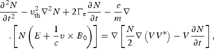 $$\eqalign{& \displaystyle{{\partial ^2 N} \over {\partial t^2}} - v_{{\rm th}}^2 \nabla ^2 N + 2\Gamma _{\rm e} \displaystyle{{\partial N} \over {\partial t}} - \displaystyle{e \over m}\nabla \cr & \quad . \left[ {N\left( {E + \displaystyle{1 \over c}v \times B_0} \right)} \right] = \nabla \left[ {\displaystyle{N \over 2}\nabla \left( {VV^{\ast}} \right) - V\displaystyle{{\partial N} \over {\partial t}}} \right],} $$
where E is the sum of electric vectors of the laser beam and self-consistent field, V is the sum of the drift velocities of the electron in the laser field and self-consistent field, Гe is the Landau damping factor, v th is the square of the electron thermal speed, and m is the relativistic mass of electrons. The equation for the generated electrostatic pulse at twice the pump frequency can be obtained from Eq. (2) by substituting
 $$N = N_3 + N_1 \,{\rm exp}(i{\rm \omega} _{\,0} t) + N_2 \,{\rm exp}(2i{\rm \omega} _{\,0} t) $$
Here we are interested in the component of the electron density (N 2), which is at the second-harmonic frequency, and is given by
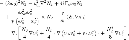 $$\eqalign{& - (2{\rm \omega} _0 )^2 N_2 - v_{{\rm th}}^2 \nabla ^2 N_2 + 4i\Gamma _{\rm e} {\rm \omega} _0 N_2 \cr & \quad + \displaystyle{{{\rm \omega} _{{\rm po}}^2 {\rm \omega} _{\rm o}^{\rm 2}} \over {{\rm \gamma} \left( {{\rm \omega} _{\rm o}^2 - {\rm \omega} _{\rm c}^2} \right)}} \times N_2 - \displaystyle{e \over m}\left( {E.\nabla n_0} \right) \cr & \quad = \nabla. \left[ {\displaystyle{{N_0} \over 4}\nabla \nu _0^2 + \displaystyle{{N_2} \over 4}\left\{ {\nabla \left( {\nu _0. \nu _0^{\ast} + \nu _2. \nu _2^{\ast}} \right)} \right\} + \displaystyle{{N_2^{\ast}} \over 8}\nabla \nu _2^2} \right],} $$
where v 0 and v 2 are the drift velocities of electron in the pump field and self-consistent field, ωc is the cyclotron frequency, n 0 is the time-independent component of electron density and relativistic factor
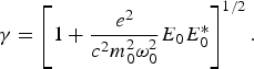 $${\rm {\rm \gamma}} = \left[ {1 + \displaystyle{{e^2} \over {c^2 m_0^2 {\rm \omega} _0^2}} E_0 E_0^{\ast}} \right]^{1/2}. $$
Further, N 2 can be written using the eikonal approximation
 $$N_2 = N_{20} (x,y,z)\,e^{ - ikz} e^{ - iks} + N_{21} (x,y,z)\,e^{ - 2ik_0 z} e^{ - 2ik_0 s_0}, $$
where N 20(x, y, z) and N 21(x, y, z) are the complex functions of their arguments and k satisfies the usual dispersion relation  ${\rm \omega} _0^2 = ({\rm \omega} _{\rm p}^2 {\rm \omega} _0^2 /({\rm \omega} _0^2 - {\rm \omega} _{\rm c}^2 )) + k^2 v_{{\rm th}}^2 $. Following the standard technique of Akhmanov et al. (Reference Akhmanov, Sukhorukov and Khokhlov1968), we separate the real and imaginary parts and separate the different phases, and we get the amplitude of the plasma wave as
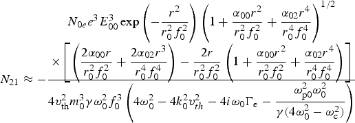 $$N_{21} \approx - \displaystyle{{\matrix{N_{0e} e^3 E_{00}^3 \,{\rm exp}\left( - \displaystyle{{r^2} \over {r_0^2 f_0^2}} \right) \left(1 + \displaystyle{{{\rm \alpha} _{00} r^2} \over {r_0^2 f_0^2}} + \displaystyle{{{\rm \alpha} _{02} r^4} \over {r_0^4 f_0^4}} \right)^{1/2} \cr \times \left[ \left( \displaystyle{{2{\rm \alpha} _{00} r} \over {r_0^2 f_0^2}} + \displaystyle{{2{\rm \alpha} _{02} r^3} \over {r_0^4 f_0^4}} \right) - \displaystyle{{2r} \over {r_0^2 f_0^2}} \left(1 + \displaystyle{{{\rm \alpha} _{00} r^2} \over {r_0^2 f_0^2}} + \displaystyle{{{\rm \alpha} _{02} r^4} \over {r_0^4 f_0^4}} \right) \right]}} \over {4v_{\rm th}^2 m_0^3 {\rm \gamma} {\rm \omega} _0^2 f_0^3 \left( 4{\rm \omega} _0^2 - 4k_0^2 v_{th}^2 - 4i{\rm \omega} _0 \Gamma _{\rm e} - \displaystyle{{{\rm \omega} _{{\rm p}0}^2 {\rm \omega} _0^2} \over {{\rm \gamma} (4{\rm \omega} _0^2 - {\rm \omega} _{\rm c}^{\rm 2} )}} \right)}} $$
Following Akhmanov et al. (Reference Akhmanov, Sukhorukov and Khokhlov1968) N 20 can be written as
 $$N_{20}^2 = \displaystyle{{B^{^{\prime}2}} \over {\,f^2}} {\rm exp}\left( {\displaystyle{{ - r^2} \over {a_0^2 f^2}}} \right){\rm exp}( - 2k_i z)\left( {1 + \displaystyle{{{\rm \alpha} _{0{\rm p}} r^2} \over {a_0^2 f^2}} + \displaystyle{{{\rm \alpha} _{2{\rm p}} r^4} \over {a_0^4 f^2}}} \right), $$
 $$S = \displaystyle{{S_{0{\rm p}}} \over {a_0^2}} + \displaystyle{{S_{2{\rm p}} r^4} \over {a_0^4}}, \quad {\rm where}\quad {\rm} S_{0{\rm p}} = \displaystyle{{r^2} \over {2f}}\displaystyle{{df} \over {dz}},$$
where B′ and a 0 are constants (to be determined by the boundary conditions that the amplitude of the generated plasma wave at z = 0 is zero)
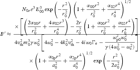 $$\eqalign{B^{\prime} \approx \displaystyle{\matrix{N_{0e} e^3 E_{00}^3 \,{\rm exp}\left( { - \displaystyle{{r^2} \over {r_0^2}}} \right)\left( {1 + \displaystyle{{{\rm \alpha} _{00} r^2} \over {r_0^2}} + \displaystyle{{{\rm \alpha} _{02} r^4} \over {r_0^4}}} \right)^{{1 / 2}}\cr \times\left[ {\left( {\displaystyle{{2{\rm \alpha} _{00} r} \over {r_0^2}} + \displaystyle{{4{\rm \alpha} _{02} r^3} \over {r_0^4}}} \right) - \displaystyle{{2r} \over {r_0^2}} \left( {1 + \displaystyle{{{\rm \alpha} _{00} r^2} \over {r_0^2}} + \displaystyle{{{\rm \alpha} _{02} r^4} \over {r_0^4}}} \right)} \right]} \over \matrix{4v_{{\rm th}}^2 m_0^3 {\rm \gamma} {\rm \omega} _0^2 \left[ {4{\rm \omega} _0^2 - 4k_0^2 v_{{\rm th}}^2 - 4i{\rm \omega} _0 \Gamma _{\rm e} - \displaystyle{{{\rm \omega} _{{\rm p}0}^2 {\rm \omega} _0^2} \over {{\rm \gamma} (4{\rm \omega} _0^2 - {\rm \omega} _{\rm c}^2 )}}} \right]\cr \times\left( {1 + \displaystyle{{{\rm \alpha} _{0{\rm p}} r^2} \over {a_0^2}} + \displaystyle{{{\rm \alpha} _{2{\rm p}} r^4} \over {a_0^4}}} \right)^{{1 / 2}} {\rm exp}\left( { - \displaystyle{{r^2} \over {2a_0^2}}} \right)}}} $$
and f is the dimensionless beam width parameter of plasma wave with the initial condition f is f = 1 and df/dz = 0 plane wave front at z = 0, governed by
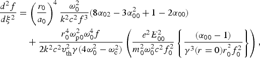 $$\eqalign{\displaystyle{{d^2 f} \over {d\xi ^2}} &= \left( {\displaystyle{{r_0} \over {a_0}}} \right)^4 \displaystyle{{{\rm \omega} _0^2} \over {k^2 c^2 f^3}} (8{\rm \alpha} _{02} - 3{\rm \alpha} _{00}^2 + 1 - 2{\rm \alpha} _{00} ) \cr & \quad + \displaystyle{{r_0^4 {\rm \omega} _{{\rm p}0}^2 {\rm \omega} _0^4 f} \over {2k^2 c^2 v_{{\rm th}}^2 {\rm \gamma} (4{\rm \omega} _0^2 - {\rm \omega} _{\rm c}^2 )}}\left( {\displaystyle{{e^2 E_{00}^2} \over {m_0^2 {\rm \omega} _0^2 c^2 f_0^2}} \left\{ {\displaystyle{{({\rm \alpha} _{00} - 1)} \over {{\rm \gamma} ^3 (r = 0)r_0 ^{^2} f_0^2}}} \right\}} \right),} $$
k i = 2Γeω0/kv th2, α0p, α2p are the contributions from the r 2 and r 4 coefficients and are the functions of z, also S 0p, S 2p are eikonal contributions for the electron plasma wave (EPW) from r 2 and r 4 coefficient in the non-paraxial region and, are functions of (r, z), a 0 is the half-width of the Gaussian distribution for the plasma wave. We have equations for S 2pα0p, α2p with initial condition and S 0p =S 2p = 0 at z = 0.
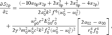 $$\eqalign{& \displaystyle{{\partial S_{2{\rm p}}} \over {\partial z}} = \displaystyle{{( - 10{\rm \alpha} _{0{\rm p}} {\rm \alpha} _{2{\rm p}} + 2{\rm \alpha} _{0{\rm p}}^3 + 2{\rm \alpha} _{0{\rm p}}^2 - 4{\rm \alpha} _{2{\rm p}} )} \over {2a_0^2 k^2 f^6 ({\rm \omega} _0^2 - {\rm \omega} _{\rm c}^2 )}} \cr & \quad + \displaystyle{{{\rm \omega} _{{\rm p}0}^2 e^2 E_{00}^2 r_0^2} \over {2{\rm {\rm \gamma}} ^3 m_0^2 {\rm \omega} _0^4 c^2 k^2 f_0^2 ({\rm \omega} _0^2 - {\rm \omega} _{\rm c}^2 )^2}} \left[ {\displaystyle{{2{\rm \alpha} _{02} - {\rm \alpha} _{00}} \over {r_0^4 f_0^4}}} \right],} $$
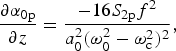 $$\displaystyle{{\partial {\rm \alpha} _{0{\rm p}}} \over {\partial z}} = \displaystyle{{ - 16S_{2{\rm p}} f^2} \over {a_0^2 ({\rm \omega} _0^2 - {\rm \omega} _{\rm c}^2 )^2}}, $$
 $$\displaystyle{{\partial {\rm \alpha} _{2{\rm p}}} \over {\partial z}} = \displaystyle{{8S_{2{\rm p}} f^2} \over {a_0^2 ({\rm \omega} _0^2 - {\rm \omega} _{\rm c}^2 )}} - \displaystyle{{24{\rm \alpha} _{0{\rm p}} S_{2{\rm p}} f^2} \over {a_0^2 ({\rm \omega} _0^2 - {\rm \omega} _{\rm c}^2 )^3}}. $$
Using Maxwell's equation
 $$\nabla. E_2 = - 4\rm \pi eN_2, $$
one can obtain the electric vector (E 2) of the plasma wave generated at the frequency 2ω0 as
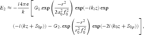 $$\eqalign{E_2 &\approx - \displaystyle{{i4\rm \pi e} \over k}\left[ G_1. {\rm exp}\left( {\displaystyle{{ - r^2} \over {2a_0^2 f_0^2}}} \right)\,{\rm exp}( - ik_i z)\,{\rm exp}\right.\cr &\quad \left.( - i(kz + S_{0p} )) - G_2. \,{\rm exp}\left( {\displaystyle{{ - r^2} \over {r_0^2 f_0^2}}} \right)\,{\rm exp}( - 2i(k_0 z + S_{0p} )) \right],} $$
where
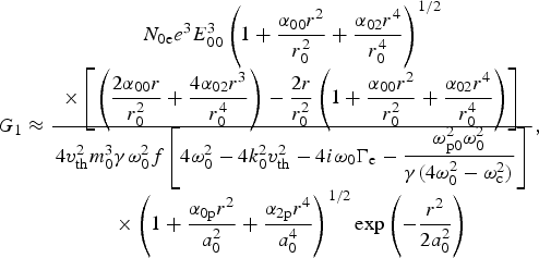 $$G_1 \approx \displaystyle{\matrix{N_{0{\rm e}} e^3 E_{00}^3 \left( {1 + \displaystyle{{{\rm \alpha} _{00} r^2} \over {r_0^2}} + \displaystyle{{{\rm \alpha} _{02} r^4} \over {r_0^4}}} \right)^{{1 / 2}}\cr \times\left[ {\left( {\displaystyle{{2{\rm \alpha} _{00} r} \over {r_0^2}} + \displaystyle{{4{\rm \alpha} _{02} r^3} \over {r_0^4}}} \right) - \displaystyle{{2r} \over {r_0^2}} \left( {1 + \displaystyle{{{\rm \alpha} _{00} r^2} \over {r_0^2}} + \displaystyle{{{\rm \alpha} _{02} r^4} \over {r_0^4}}} \right)} \right]} \over \matrix{4v_{{\rm th}}^2 m_0^3 {\rm {\rm \gamma}} {\rm \omega} _0^2 f\left[ {4{\rm \omega} _0^2 - 4k_0^2 v_{{\rm th}}^2 - 4i{\rm \omega} _0 \Gamma _{\rm e} - \displaystyle{{{\rm \omega} _{{\rm p}0}^2 {\rm \omega} _0^2} \over {{\rm \gamma} (4{\rm \omega} _0^2 - {\rm \omega} _{\rm c}^2 )}}} \right]\cr \times\left( {1 + \displaystyle{{{\rm \alpha} _{0{\rm p}} r^2} \over {a_0^2}} + \displaystyle{{{\rm \alpha} _{2{\rm p}} r^4} \over {a_0^4}}} \right)^{{1 / 2}} {\rm exp}\left( { - \displaystyle{{r^2} \over {2a_0^2}}} \right)}},$$
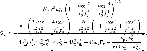 $$\eqalign{G_2 &\approx - \displaystyle{\matrix{N_{0{\rm e}} e^3 E_{00}^3 \left( {1 + \displaystyle{{{\rm \alpha} _{00} r^2} \over {r_0^2 f_0^2}} + \displaystyle{{{\rm \alpha} _{02} r^4} \over {r_0^4 f_0^4}}} \right)^{{1 / 2}} \cr \times\left[ {\left( {\displaystyle{{2{\rm \alpha} _{00} r} \over {r_0^2 f_0^2}} + \displaystyle{{4{\rm \alpha} _{02} r^3} \over {r_0^4 f_0^4}}} \right) - \displaystyle{{2r} \over {r_0^2 f_0^2}} \left( {1 + \displaystyle{{{\rm \alpha} _{00} r^2} \over {r_0^2 f_0^2}} + \displaystyle{{{\rm \alpha} _{02} r^4} \over {r_0^4 f_0^4}}} \right)} \right]} \over {4v_{{\rm th}}^2 m_0^3 {\rm {\rm \gamma}} {\rm \omega} _0^2 f_0^3 \left[ {4{\rm \omega} _0^2 - 4k_0^2 v_{{\rm th}}^2 - 4i{\rm \omega} _0 \Gamma _{\rm e} - \displaystyle{{{\rm \omega} _{{\rm p}0}^2 {\rm \omega} _0^2} \over {{\rm \gamma} (4{\rm \omega} _0^2 - {\rm \omega} _{\rm c}^2 )}}} \right]}}.}$$
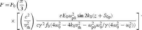
The power of plasma wave at twice the pump wave frequency, incident across the transverse cross-section at z can be obtained by integrating E 2E 2* over r from 0 to ∞, that is,
 $$\eqalign{P = & P_0 \left( {\displaystyle{\rm \pi \over 3}} \right) \cr & \times \left[ {\left( {\displaystyle{{c^2} \over {v_{{\rm th}}^2}}} \right)\displaystyle{{eE_0 {\rm \omega} _{{\rm p}0}^2 \sin 2k_0 (z + S_{0{\rm p}} )} \over {c{\rm \gamma} ^2 f_0 (4{\rm \omega} _0^2 - 4k_0 v_{{\rm th}}^2 - {{{\rm \omega} _{{\rm p}0}^2 {\rm \omega} _0^2} / {{\rm \gamma} (4{\rm \omega} _0^2 - {\rm \omega} _{\rm c}^2 )}})}}} \right]}. $$
Above expression shows the power of the plasma wave across the transverse cross-section. Equation (17) can be solved along with the numerical computation of Eq. (15) with the help of Eq. (16a) and (16b) to obtain the variation in the power of plasma wave.
3. THIRD-HARMONIC GENERATION
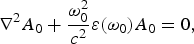
As discussed above, the plasma wave is generated at twice the pump frequency. This plasma wave can interact with the incident laser beam and the third-harmonic can be generated. Using Eq. (1) one can obtain the third-harmonic field by laser beam. Equation (1) splits up in terms of vector potential for the fundamental (A 0) and the third-harmonic generation (A 3) as
 $$\nabla ^2 A_0 + \displaystyle{{{\rm \omega} _0^2} \over {c^2}} {\rm \varepsilon} ({\rm \omega} _0 )A_0 = 0, $$
 $$\nabla ^2 A_3 + \displaystyle{{{\rm \omega} _3^{^2}} \over {c^2}} {\rm \varepsilon} _3 ({\rm \omega} _3 )A_3 = \displaystyle{{{\rm \omega} _{{\rm p}0}^2} \over {2c^2}} \displaystyle{{N_2} \over {n_0}} A_0, $$
where ω 3 = ω0 + 2ω0, ε(ω0), and ε3(ω 3) are the effective dielectric constants of the plasma at the fundamental and third-harmonic frequency.
Now the effective dielectric constant of the plasma at frequency ω0 is given by
 $${\rm \varepsilon} ({\rm \omega} _0 ) = {\rm \varepsilon} _0 ({\rm \omega} _0 ) + {\rm \phi} (E_0. E_0^{\ast}), $$
where
 $${\rm \phi} (E_0. E_0^{\ast}) = \displaystyle{{{\rm \omega} _{\rm p}^2} \over {{\rm \omega} _0 ({\rm \omega} _0 - {\rm \omega} _{\rm c} )}}\left( {1 - \displaystyle{1 \over {\rm {\rm \gamma}}}} \right). $$
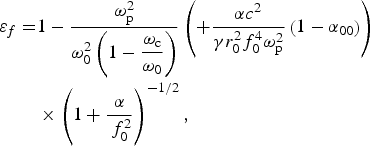
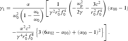
Expending dielectric constant around r = 0 by Taylor expansion, one can write
 $${\rm \varepsilon} ({\rm \omega} _0 ) = {\rm \varepsilon} _f ({\rm \omega} _0 ) + {\rm {\rm \gamma}} _1 ({\rm \omega} _0 )r^2, $$
where
 $$\eqalign{{\rm \varepsilon} _f = & 1 - \displaystyle{{{\rm \omega} _{\rm p}^2} \over {{\rm \omega} _0^2 \left( {1 - \displaystyle{{{\rm \omega} _{\rm c}} \over {{\rm \omega} _0}}} \right)}}\left( { + \displaystyle{{{\rm \alpha} c^2} \over {{\rm {\rm \gamma}} r_0^2 f_0^4 {\rm \omega} _{\rm p}^2}} \left( {1 - {\rm \alpha} _{00}} \right)} \right)\cr & \times \left( {1 + \displaystyle{{\rm \alpha} \over {\,f_0^2}}} \right)^{ - {1 / 2}},} $$
 $$\eqalign{{\rm \gamma} _1 &= \displaystyle{{\rm \alpha} \over {{\rm \omega} _0^2 \left( {1 - \displaystyle{{{\rm \omega} _{\rm c}} \over {{\rm \omega} _0}}} \right)}}\left[ \displaystyle{1 \over {{\rm \gamma} ^2 r_0^2 f_0^4}} \left( { - \displaystyle{{{\rm \omega} _{\rm p}^2} \over {2{\rm \gamma}}} - \displaystyle{{3c^2} \over {r_0^2 f_0^4}}} \right)\left( {{\rm \alpha} _{00} - 1} \right)\right.\cr &\quad \left. - \displaystyle{{{\rm \alpha} ^2 c^2} \over {{\rm {\rm \gamma}} ^4 r_0^4 f_0^8}} \left\{ {3\left( {6{\rm \alpha} _{02} - {\rm \alpha} _{00}} \right) + \left( {{\rm \alpha} _{00} - 1} \right)^2} \right\} \right].} $$
The effective dielectric constant of the plasma at the third-harmonic frequency is given by
 $${\rm \varepsilon} _3 ({\rm \omega} _3 ) = {\rm \varepsilon} _{3f} ({\rm \omega} _3 ) + {\rm \gamma} _3 ({\rm \omega} _3 )r^2, $$
where
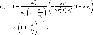 $$\eqalign{{\rm \varepsilon} _{3f} \, = & \,1 - \displaystyle{{{\rm \omega} _{\rm p}^2} \over {{\rm \omega} _3^2 \left( {1 - \displaystyle{{{\rm \omega} _{\rm c}} \over {{\rm \omega} _3}}} \right)}}\left( { + \displaystyle{{{\rm \alpha} c^2} \over {{\rm \gamma} r_0^2 f_0^4 {\rm \omega} _p^2}} \left( {1 - {\rm \alpha} _{00}} \right)} \right) \cr & \times \left( {1 + \displaystyle{{\rm \alpha} \over {\,f_0^2}}} \right)^{ - {1 / 2}},} $$
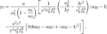 $$\eqalign{{\rm {\rm \gamma}} _3 &= \displaystyle{{\rm \alpha} \over {{\rm \omega} _3^2 \left( {1 - \displaystyle{{{\rm \omega} _{\rm c}} \over {{\rm \omega} _3}}} \right)}}\left[ \displaystyle{1 \over {{\rm \gamma} ^2 r_0^2 f_0^4}} \left( { - \displaystyle{{{\rm \omega} _{\rm p}^2} \over {2{\rm \gamma}}} - \displaystyle{{3c^2} \over {r_0^2 f_0^4}}} \right)({\rm \alpha} _{00} - 1)\right. \cr &\left. - \displaystyle{{{\rm \alpha} ^2 c^2} \over {{\rm {\rm \gamma}} ^4 r_0^4 f_0^8}} \left\{ {3(6{\rm \alpha} _{02} - {\rm \alpha} _{00} ) + ({\rm \alpha} _{00} - 1)^2} \right\} \right],} $$
where  ${\rm \alpha} = {{e^2} / {m^2 c^4}} A_{00}^2 $. Equation (18) may be solved using the standard techniques of Akhmanov et al. (Reference Akhmanov, Sukhorukov and Khokhlov1968) where the laser electric field A 0 and eikonal S 0 are given by
 $$A_0 = \left( {1 + \displaystyle{{{\rm \alpha} _{00} r^2} \over {r_0^2 f_0^2}} + \displaystyle{{{\rm \alpha} _{02} r^4} \over {r_0^4 f_0^4}}} \right)^{{1 / 2}} \displaystyle{{E_{00}} \over {\,f_0}} \exp \left( {\displaystyle{{ - r^2} \over {2r_0^2 f_0^2}}} \right), $$
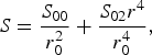 $$S = \displaystyle{{S_{00}} \over {r_0^2}} + \displaystyle{{S_{02} r^4} \over {r_0^4}} {\rm,} $$
where
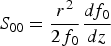 $$S_{00} = \displaystyle{{r^2} \over {2f_0}} \displaystyle{{df_0} \over {dz}}$$
f 0 is governed with the initial condition df 0/dz = 0, f 0 = 1 at z = 0 and can be written as
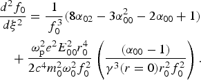 $$\eqalign{& \displaystyle{{d^2 f_0} \over {d\rm \xi ^2}} = \displaystyle{1 \over {\,f_0^3}} (8{\rm \alpha} _{02} - 3{\rm \alpha} _{00}^2 - 2{\rm \alpha} _{00} + 1) \cr & \quad + \displaystyle{{{\rm \omega} _{\rm p}^2 e^2 E_{00}^2 r_0^4} \over {2c^4 m_0^2 {\rm \omega} _0^2 f_0^2}} \left( {\displaystyle{{({\rm \alpha} _{00} - 1)} \over {{\rm {\rm \gamma}} ^3 (r = 0)r_0^2 f_0^2}}} \right).} $$
We obtain the following equation:
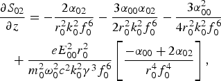 $$\eqalign{& \displaystyle{{\partial S_{02}} \over {\partial z}} = - \displaystyle{{2{\rm \alpha} _{02}} \over {r_0^2 k_0^2 f_0^6}} - \displaystyle{{3{\rm \alpha} _{00} {\rm \alpha} _{02}} \over {2r_0^2 k_0^2 f_0^6}} - \displaystyle{{3{\rm \alpha} _{00}^2} \over {4r_0^2 k_0^2 f_0^6}} \cr & \quad + \displaystyle{{eE_{00}^2 r_0^2} \over {m_0^2 {\rm \omega} _0^2 c^2 k_0^2 {\rm {\rm \gamma}} ^3 f_0^6}} \left[ {\displaystyle{{ - {\rm \alpha} _{00} + 2{\rm \alpha} _{02}} \over {r_0^4 f_0^4}}} \right],} $$
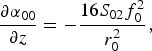 $$\displaystyle{{\partial {\rm \alpha} _{00}} \over {\partial z}} = - \displaystyle{{16S_{02} f_0^2} \over {r_0^2}}, $$
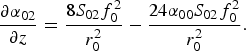 $$\displaystyle{{\partial {\rm \alpha} _{02}} \over {\partial z}} = \displaystyle{{8S_{02} f_0^2} \over {r_0^2}} - \displaystyle{{24{\rm \alpha} _{00} S_{02} f_0^2} \over {r_0^2}}. $$
Further, the solution for A 3 can be written as
 $$A_3 = A_{30} (r,z)\,{\rm exp}( - i(k_3 z + S_3 )) + A_{31} (r,z)\,{\rm exp}( - 3i(k_0 z + S_0 )). $$
The expression for A 31 is obtained as
 $$\eqalign{& A_{31} \cong \displaystyle{{{\rm \omega} _{{\rm p}0}^2} \over {2c^2}} \displaystyle{{{\rm \omega} _3} \over {{\rm \omega} _0}} \left( {\displaystyle{{N_{12}^{\prime}} \over {n_0}}} \right)\displaystyle{{E_{00}} \over {\,f_0}} \left( {1 + \displaystyle{{{\rm \alpha} _{0{\rm h}} r^2} \over {b_0^2 f_3^2}} + \displaystyle{{{\rm \alpha} _{3{\rm h}} r^4} \over {b_0^4 f_3^4}}} \right)^{{1 / 2}} \displaystyle{{{\rm exp}({{ - r^2} / {b_0^2 f_3^2}} )} \over {(k_3^2 - 9k_0^2 )}}.} $$
Then we can solve Eq. (33) by assuming A 30 as
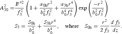 $$\eqalign{A_{30}^2 = & \displaystyle{{{B^{{\prime \prime}2}}} \over {\,f_3^2 }}\left( {1 + \displaystyle{{{{\rm \alpha} _{0{\rm h}}}{r^2}} \over {b_0^2 f_3^2 }} + \displaystyle{{{{\rm \alpha} _{{\rm 3h}}}{r^4}} \over {b_0^4 f_3^4 }}} \right){\rm exp}\left( {\displaystyle{{ - {r^2}} \over {b_0^2 f_3^2 }}} \right) \cr & {S_3} = \displaystyle{{{S_{0{\rm h}}}} \over {b_0^2 }} + \displaystyle{{{S_{{\rm 3h}}}{r^4}} \over {b_0^4 }},\quad {\rm where}\quad {\rm }{S_{{\rm 0h}}} = \displaystyle{{{r^2}} \over {2{\,f_3}}}\displaystyle{{d{\,f_3}} \over {dz}}.}$$
α0h and α3h are the contributions from r 2 and r 4 coefficients and are the functions of z in the modified-paraxial region, S 0h and S 3h are the eikonal contributions from r 2 and r 4 coefficients and are the functions of (r, z), here b 0 is the third-harmonic beam width. Using initial conditions, df 3/dz = 0, f 3 = 1 at z = 0, and solving for α0h and α3h in similar way as we did in the previous section, the dimensionless beam width parameter f 3 of third-harmonic radiation is governed by
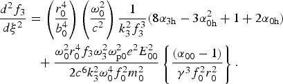 $$\eqalign{& \displaystyle{{d^2 f_3} \over {d\rm \xi ^2}} = \left( {\displaystyle{{r_0^4} \over {b_0^4}}} \right)\left( {\displaystyle{{{\rm \omega} _0^2} \over {c^2}}} \right)\displaystyle{1 \over {k_3^2 f_3^3}} (8{\rm \alpha} _{3{\rm h}} - 3{\rm \alpha} _{0{\rm h}}^2 + 1 + 2{\rm \alpha} _{0{\rm h}} ) \cr & \qquad\quad + \displaystyle{{{\rm \omega} _0^2 r_0^4 f_3 {\rm \omega} _3^2 {\rm \omega} _{{\rm p}0}^2 e^2 E_{00}^2} \over {2c^6 k_3^2 {\rm \omega} _0^4 f_0^2 m_0^2}} \left\{ {\displaystyle{{({\rm \alpha} _{00} - 1)} \over {{\rm \gamma} ^3 f_0^2 r_0^2}}} \right\}.} $$
The constant B″ and b 0 are also determined by the boundary condition that the third-harmonic generation is zero at z = 0
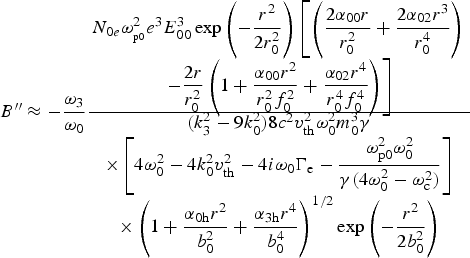 $$\eqalign{B^{\prime\prime} &\approx - \displaystyle{{{\rm \omega} _3} \over {{\rm \omega} _0}} \displaystyle{\matrix{N_{0e} {\rm \omega} _{_{{\rm p0}}} ^2 e^3 E_{00}^3 \,{\rm exp}\left( { - \displaystyle{{r^2} \over {2r_0^2}}} \right) \left[ \left( {\displaystyle{{2{\rm \alpha} _{00} r} \over {r_0^2}} + \displaystyle{{2{\rm \alpha} _{02} r^3} \over {r_0^4}}} \right)\right. \cr \left.- \displaystyle{{2r} \over {r_0^2}} \left( {1 + \displaystyle{{{\rm \alpha} _{00} r^2} \over {r_0^2 f_0^2}} + \displaystyle{{{\rm \alpha} _{02} r^4} \over {r_0^4 f_0^4}}} \right) \right]} \over {\matrix{(k_3^2 - 9k_0^2 )8c^2 v_{{\rm th}}^2 {\rm \omega} _0^2 m_0^3 {\rm \gamma} \cr \times\left[ {4{\rm \omega} _0^2 - 4k_0^2 v_{{\rm th}}^2 - 4i{\rm \omega} _0 \Gamma _{\rm e} - \displaystyle{{{\rm \omega} _{{\rm p}0}^2 {\rm \omega} _0^2} \over {{\rm \gamma} (4{\rm \omega} _0^2 - {\rm \omega} _{\rm c}^2 )}}} \right]\cr \times\left( {1 + \displaystyle{{{\rm \alpha} _{0{\rm h}} r^2} \over {b_0^2}} + \displaystyle{{{\rm \alpha} _{3{\rm h}} r^4} \over {b_0^4}}} \right)^{{1 / 2}} {\rm exp}\left( { - \displaystyle{{r^2} \over {2b_0^2}}} \right)}}}} $$
and b 0 = r 0
Using Eqs. (34)–(37) in Eq. (33), we get
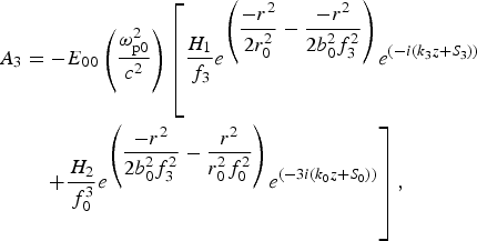 $$\eqalign{A_3 &= - E_{00} \left( {\displaystyle{{{\rm \omega} _{{\rm p}0}^2} \over {c^2}}} \right)\left[ \displaystyle{{H_1} \over {\,f_3}} e^{\left( {\displaystyle{{ - r^2} \over {2r_0^2}} - \displaystyle{{ - r^2} \over {2b_0^2 f_3^2}}} \right)} e^{\left( { - i\left( {k_3 z + S_3} \right)} \right)}\right. \cr &\quad \left. + \displaystyle{{H_2} \over {\,f_0^3}} e^{\left( {\displaystyle{{ - r^2} \over {2b_0^2 f_3^2}} - \displaystyle{{r^2} \over {r_0^2 f_0^2}}} \right)} e^{\left( { - 3i\left( {k_0 z + S_0} \right)} \right)} \right],} $$
where
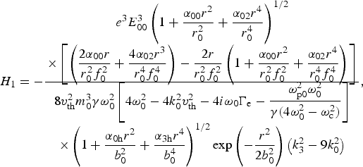 $$\eqalign{H_1 = - \displaystyle{\matrix{e^3 E_{00}^3 \left( {1 + \displaystyle{{{\rm \alpha} _{00} r^2} \over {r_0^2}} + \displaystyle{{{\rm \alpha} _{02} r^4} \over {r_0^4}}} \right)^{{1 / 2}}\cr \times\left[ {\left( {\displaystyle{{2{\rm \alpha} _{00} r} \over {r_0^2 f_0^2}} + \displaystyle{{4{\rm \alpha} _{02} r^3} \over {r_0^4 f_0^4}}} \right) - \displaystyle{{2r} \over {r_0^2 f_0^2}} \left( {1 + \displaystyle{{{\rm \alpha} _{00} r^2} \over {r_0^2 f_0^2}} + \displaystyle{{{\rm \alpha} _{02} r^4} \over {r_0^4 f_0^4}}} \right)} \right]} \over \matrix{8v_{{\rm th}}^2 m_0^3 {\rm {\rm \gamma}} {\rm \omega} _0^2 \left[ {4{\rm \omega} _0^2 - 4k_0^2 v_{{\rm th}}^2 - 4i{\rm \omega} _0 \Gamma _{\rm e} - \displaystyle{{{\rm \omega} _{{\rm p}0}^2 {\rm \omega} _0^2} \over {{\rm \gamma} (4{\rm \omega} _0^2 - {\rm \omega} _{\rm c}^2 )}}} \right]\cr \times\left( {1 + \displaystyle{{{\rm \alpha} _{0{\rm h}} r^2} \over {b_0^2}} + \displaystyle{{{\rm \alpha} _{3{\rm h}} r^4} \over {b_0^4}}} \right)^{{1 / 2}} {\rm exp}\left( { - \displaystyle{{r^2} \over {2b_0^2}}} \right)\left( {k_3^2 - 9k_0^2} \right)}},}$$
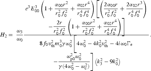 $$\eqalign{H_2 &= \,\displaystyle{{{\rm \omega} _3} \over {{\rm \omega} _0}} \displaystyle{\matrix{e^3 E_{00}^3 \left( {1 + \displaystyle{{{\rm \alpha} _{00} r^2} \over {r_0^2 f_0^2}} + \displaystyle{{{\rm \alpha} _{02} r^4} \over {r_0^4 f_0^4}}} \right)\left[ \left( {\displaystyle{{2{\rm \alpha} _{00} r} \over {r_0^2 f_0^2}} + \displaystyle{{2{\rm \alpha} _{02} r^3} \over {r_0^4 f_0^4}}} \right)\right.\cr \left.- \displaystyle{{2r} \over {r_0^2 f_0^2}} \left( {1 + \displaystyle{{{\rm \alpha} _{00} r^2} \over {r_0^2 f_0^2}} + \displaystyle{{{\rm \alpha} _{02} r^4} \over {r_0^4 f_0^4}}} \right) \right]} \over \matrix{ 8f_0 v_{{\rm th}}^2 m_0^3 {\rm {\rm \gamma}} {\rm \omega} _0^2 \left[\vphantom{\displaystyle{{{\rm \omega} _{{\rm p}0}^2 {\rm \omega} _0^2} \over {{\rm \gamma} (4{\rm \omega} _0^2 - {\rm \omega} _{\rm c}^2 )}}} 4{\rm \omega} _0^2 - 4k_0^2 v_{{\rm th}}^2 - 4i{\rm \omega} _0 \Gamma _{\rm e}\right. \cr \left. - \displaystyle{{{\rm \omega} _{{\rm p}0}^2 {\rm \omega} _0^2} \over {{\rm \gamma} (4{\rm \omega} _0^2 - {\rm \omega} _{\rm c}^2 )}} \right]\left( {k_3^2 - 9k_0^2} \right)}}.}$$
Therefore the third-harmonic power P 3 incident across the transverse cross-section at z comes out as
 $$\eqalign{& P_3 \approx P_0 \left( {\displaystyle{{{\rm \omega} _{{\rm po}}} \over {c^2}}} \right)^2 \times \left[ {\displaystyle{{H_1^2} \over {2(1 + f_3^2 )}} + \displaystyle{{H_2^2} \over {4f_0^4}} + \displaystyle{{2H_1 H_2 f_3 \cos \left[ {(k_3 - 3k_0 )z} \right]} \over {\left[ {\,f_0^2 (1 + f_3^2 ) + 2f_3^2} \right]}}} \right].} $$
We have solved Eq. (32) numerically for the same set of the parameters used in Section 2 and the results are shown in Figure 4.
4. DISCUSSIONS
In order to study the plasma wave excitation and harmonic generation in the relativistic magneto plasma, we have considered collisionless magneto plasma in which a laser beam is considered to be propagated. It is very well known that during the propagation of laser beam in the plasma the density of the plasma is considered to be varied due to the relativistic mass change of the electron and the refractive index of the medium increases at the position of maximum irradiance of the laser beam and the laser gets focused in the plasma. The intensity profile of the laser beam in the plasma is shown by Eq. (28) along the radial direction. The focusing/defocusing activity of laser beams is subjective to the magnitudes of the nonlinear coupling term of Eq. (29).
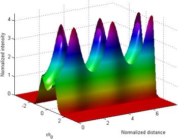
To show the intensity profile of the laser beam in the plasma, we made computations of Eq. (28) with the help of Eqs (28)–(32). These coupled equations are solved for the initial wave front of the laser beam. For the initial plane wave front of the beam, the initial conditions for laser beam width parameter f 0 are f 0 = 1 and df 0/dz = 0, S 00 = S 02 = 0 at z = 0. Figure 1 shows the intensity profile of the laser beam. It is obvious form the figure that laser beam travels with split profile as the restriction of paraxial approximation is relaxed on the laser beam profile. The calculations are done with the typical laser, plasma parameters: [The vacuum wavelength of the laser beam (λ = 1064 nm), the initial radius of the laser beam (18 μm), laser power flux (1018 W/cm2) at plasma density (ωp = 0.2ω0), and (υ th = 0.1c)].
Variation in laser beam intensity with normalized distance ξ(=zc/ω0r 02) and radial distance (r) for laser power when relativistic nonlinearity is operative.

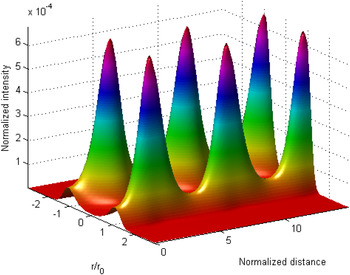
For the purpose of study of the plasma wave excitation, we have solved Eq. (8) numerically with the help of Eqs (9)–(13) to obtain the amplitude of the density perturbation at finite z. The profile of EPW depends on the beam width parameters f and the coefficients (α0p and α2p) of r 2 and r 4 in the modified-paraxial region. Figure 2 shows the profile of the EPW, when relativistic nonlinearity is operative for typical laser parameters as we have used above in this section. The nonlinear coupling between the high-power laser beam and seed plasma wave leads to the excitation of plasma wave. This coupling is so strong that the initial plasma wave is localized. The behavior of EPW as shown in Figure 2 can be explained using Eq. (10), in which the electric field vector of the plasma wave depend on the beam width parameter of the laser beam f 0 and on the other coefficients (α00 andα02) in a very complex way. Figure 2 depicts that the EPW is also having the split profile with minimum power on the axis. It is clearly shown in the figure that the EPW has the maxima at those points where the laser beam is focused (as shown in Fig. 1).
Variation in plasma wave intensity with normalized distance ξ(=zc/ω0r 02) and radial distance (r) for laser power when relativistic nonlinearity is operative.

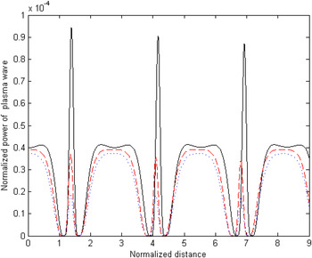
However, to appreciate the dependence of the power of plasma wave on magnetic field, we have solved Eq. (17) numerically along with the numerical computation of Eq. (15) with the help of Eqs. (16a) and (16b) to obtain the variation in the power of plasma wave. Results are presented in the form of Figure 3. Figure 3 displays the variation of the dimensionless power of the plasma wave with the normalized distance of propagation with different strengths of the magnetic field. When the laser beam propagates in the plasma, the plasma wave gets excited due to nonlinear coupling with high-power laser beam because of the relativistic nonlinearity. This ultra-intense laser beam interacts with plasma electrons and these electrons will gain momentum, but the mass of electron will be increased due to relativistic effect, and their dynamics will be influenced. This coupling is so strong that the initial plasma wave becomes highly localized, and this will change the electron density of the plasma channel. It is evident from the figure that the plasma wave power is significantly affected with the distance of propagation. It is seen from the figure that as the strength of magnetic field increases the power of plasma wave decrease.
Variation in plasma wave power normalized by the power of the incident beam |P|/|P 0| with normalized distance ξ(=zc/ω0r 02), when relativistic nonlinearity is operative for different values of ωc/ω0. Black solid, red dashed, and blue dotted line are, respectively, for ωc/ω0 = 0.16, ωc/ω0 = 0.34, and ωc/ω0 = 0.52.

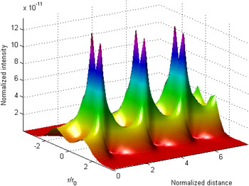
The theory of the third-harmonic generation is developed when relativistic nonlinearity is operative. Moreover, the efficiency of the harmonic generation process is significantly affected due to the phase mismatch between the fundamental and generated harmonic radiation. We have solved Eq. (38) numerically for the same set of the parameters and plotted the graph showing the intensity of the third-harmonics for normalized distance and radial distance. The result is shown in the form of Figure 4. Figure 4 shows the variation of the intensity of the third-harmonics with normalized distance and the radial distance. It is clearly shown in the figure that the third-harmonic wave also follows the split pattern in the extended-paraxial region. It is evident from Eq. (35) that the third-harmonic intensity depends upon coefficient B″ and beam width parameter of third-harmonic wave. Further, the third-harmonic beam width parameter is governed by Eq. (36) and the coefficient B″ is given by Eq. (37). Now we can see that A 30 will be maximum when B″ will be maximum. We can explain the same on the basis of the fact that Figure 4 shows the maximum intensity at the point where the phase matching condition is satisfied and vice versa. In Figure 4, when the amplitude reaches the maximum it demands the condition k 3 = 3k 0; the condition k 3 = 3k 0 makes the analytical value of A 31 the highest. Similarly, the value of B″ will be highest when k 3 = 3k 0. Thus the condition k 3 = 3k 0 makes the maximum value of A 3 maximum being H 1 and H 2 maximum. In addition to that dependence of f 3 on relativistic factor γ also makes the relativistic dependence of the intensity of the third-harmonic. However, it was shown that the second- and third-harmonic emitted from the plasma had the characteristic angular distributions and the process is expected to be incoherent. Interest in this process has continued because it offers the possibility of studying some of the basic physics of the interaction of relativistic electrons with strong fields, with possible applications to processes occurring in astrophysical plasmas. In the present work, we want to study rough estimate of the change in the third-harmonic efficiency with the change in magnetic field considering the relativistic nonlinearity only.
Variation in the third-harmonic intensity with normalized distance ξ(=zc/ω0r 02) and radial distance (r) for laser power when relativistic nonlinearity is operative.

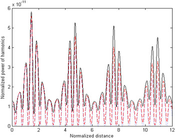
We have solved Eq. (40) numerically for the same set of the parameters used in Section 2 and the results are shown in Figure 5. Figure 5 shows the variation of third-harmonic power (normalized by the pump wave power) with the normalized distance of propagation with different strengths of magnetic field. As discussed above the plasma wave power is significantly affected with the distance of propagation and hence the power of third-harmonic is also considerably modified.
Variation in the third-harmonic power normalized by the power of the incident beam |P 3|/|P 0| with normalized distance ξ(=zc/ω0r 02), when relativistic nonlinearity is operative in modified – paraxial region for different values of ωc/ω0. Black solid, red dashed, and blue dotted line are, respectively, for ωc/ω0 = 0.16, ωc/ω0 = 0.34, and ωc/ω0 = 0.52.

5. CONCLUSION
In summary, we have studied that the plasma wave generation can be a considerable process for third-harmonic generation in magneto plasma along with the effect of relativistic nonlinearity within the modified paraxial ray approximation. We have observed the effect of relativistic nonlinearity on the propagation of pump beam and plasma wave excitation. The coupling term between intense laser beam and plasma wave due to relativistic nonlinearity with modified-paraxial approximation has been derived. The third-harmonic power as a result of this plasma wave has considerable magnitude and the influence of the magnetic field on third-harmonic power is investigated. It is observed that with the change in the magnitude of magnetic field strength the power of plasma wave generation and the third-harmonic generation is significantly affected.
ACKNOWLEDGMENT
This work was partially supported by the University Grant Commission (UGC), (F. No. 42-820/2013 SR) New Delhi, India. The author is also grateful to Professor R.P. Sharma, IIT, Delhi for his guidance.