2.1. Governing equations

In many liquid film flows, there are two-dimensional (2-D) and three-dimensional (3-D) disturbance waves. For example, some experiments of falling films show that initially, the waves are 2-D, with straight wave fronts. But transverse modulations grow as the waves travel downstream, so the wave become 3-D (Liu, Schneider & Gollub Reference Liu, Schneider and Gollub1995; Park & Nosoko Reference Park and Nosoko2003; Nosoko & Miyara Reference Nosoko and Miyara2004; Kalliadasis et al. Reference Kalliadasis, Ruyer-Quil, Scheid and Velarde2011). Thus 3-D analysis is considered suitable to scrutinise the dynamics of an arbitrary liquid film (Tomlin, Papageorgiou & Pavliotis Reference Tomlin, Papageorgiou and Pavliotis2017).

However, the disturbance waves can be considered 2-D in some region according to our experimental observations (figure 23 and supplementary movie 1). Thus in the present work, we restrict ourselves to 2-D flows with Cartesian coordinates (x, z). The dimensionless governing equations are

(2.2a) \begin{align}&\qquad\qquad\qquad\qquad \frac{\partial u}{\partial x}+\frac{\partial w}{\partial z}=0, \end{align}

(2.2b) \begin{align}&\quad\,\, \textit{Re}\left(\frac{\partial u}{\partial t}+u\frac{\partial u}{\partial x}+w\frac{\partial u}{\partial z}\right)=-\frac{\partial p}{\partial x}+\frac{\partial ^{2}u}{\partial x^{2}}+\frac{\partial ^{2}u}{\partial z^{2}}, \end{align}

(2.2c) \begin{align}& \textit{Re}\left(\frac{\partial w}{\partial t}+u\frac{\partial w}{\partial x}+w\frac{\partial w}{\partial z}\right)=-\frac{\partial p}{\partial z}+\frac{\partial ^{2}w}{\partial x^{2}}+\frac{\partial ^{2}w}{\partial z^{2}}-G. \end{align}

Here, (u, $ w $ ) and p stand for the velocity and pressure. The boundary conditions are

(2.3) \begin{equation} u=w=0\quad\mathrm{on}\ z=0, \end{equation}

and

(2.4a) \begin{align}&\qquad\qquad \partial _{t}\eta +u \boldsymbol{\cdot} \partial _{x}\eta =w, \\[-9pt] \nonumber \end{align}

(2.4b) \begin{align}& {-}p+\boldsymbol{n} \boldsymbol{\cdot} \boldsymbol{\tau } \boldsymbol{\cdot} \boldsymbol{n}=-\textit{Ca}^{-1}\,(\boldsymbol{\nabla} _{s} \boldsymbol{\cdot} \boldsymbol{n}), \\[-9pt] \nonumber \end{align}

(2.4c) \begin{align}&\qquad\qquad\quad \boldsymbol{t} \boldsymbol{\cdot} \boldsymbol{\tau } \boldsymbol{\cdot} \boldsymbol{n}=1, \end{align}

on the free surface $z=\eta (x,t)$ , where

(2.5a) \begin{align}& \boldsymbol{\tau }=\boldsymbol{\nabla }\boldsymbol{u}+\left(\boldsymbol{\nabla }\boldsymbol{u}\right)^{\mathrm{T}}, \quad \boldsymbol{\nabla} _{s}=\left(\boldsymbol{I}-\boldsymbol{nn}\right) \boldsymbol{\cdot} \boldsymbol{\nabla }, \quad \boldsymbol{\nabla} _{s} \boldsymbol{\cdot} \boldsymbol{n}= -\frac{1}{\sqrt{E^{3}}}\frac{\partial ^{2}\eta }{\partial x^{2}}, \end{align}

(2.5b) \begin{align}&\quad \boldsymbol{n}=\frac{1}{\sqrt{E}}\left(-\frac{\partial \eta }{\partial x},1\right),\quad \boldsymbol{t}=\frac{1}{\sqrt{E}}\left(1,\frac{\partial \eta }{\partial x}\right),\quad E=1+\left(\frac{\partial \eta }{\partial x}\right)^{2} \!. \end{align}

2.2. Long-wave approximation

The long-wave approximation is used in the investigation of surface waves, i.e $\varpi = d/l \ll 1$ . A scale transformation on the parameters is performed:

(2.6) \begin{equation} x=\varpi ^{-1}X,\quad z=Z,\quad u=U,\quad w=\varpi W,\quad p = \textit{Re} \boldsymbol{\cdot} P,\quad t=\varpi ^{-1}\widetilde{t} . \end{equation}

Thus the governing equations (2.2)–(2.5) can be written as

(2.7a) \begin{align}&\qquad\qquad\qquad\qquad\qquad\qquad \frac{\partial U}{\partial X}+\frac{\partial W}{\partial Z}=0, \\[-9pt] \nonumber \end{align}

(2.7b) \begin{align}&\quad\,\, \varpi\, \textit{Re}\left(\frac{\partial U}{\partial \tilde{t}}+U\frac{\partial U}{\partial X}+W\frac{\partial U}{\partial Z}\right)=-\varpi\, \textit{Re}\,\frac{\partial P}{\partial X}+\varpi ^{2}\frac{\partial ^{2}U}{\partial X^{2}}+\frac{\partial ^{2}U}{\partial Z^{2}}, \\[-9pt] \nonumber \end{align}

(2.7c) \begin{align}& \varpi ^{2}\,\textit{Re}\left(\frac{\partial W}{\partial \tilde{t}}+U\frac{\partial W}{\partial X}+W\frac{\partial W}{\partial Z}\right)=-\textit{Re}\,\frac{\partial P}{\partial Z}+\varpi ^{3}\frac{\partial ^{2}W}{\partial X^{2}}+\varpi \frac{\partial ^{2}W}{\partial Z^{2}}-G, \end{align}

while the boundary conditions are

(2.8a,b) \begin{equation} U=W=0\quad\mathrm{on}\ Z=0, \end{equation}

and those on the free surface $Z=\eta (X,\widetilde{t})$ are

(2.9a) \begin{align}&\qquad\qquad\qquad\qquad\qquad\qquad\qquad W=\frac{\partial \eta }{\partial \tilde{t}}+U\frac{\partial \eta }{\partial X},\\[-9pt] \nonumber \end{align}

(2.9b) \begin{align}&\quad -\textit{Re}\left(1+\varpi ^{2}\left(\frac{\partial \eta }{\partial X}\right)^{2}\right)P+2\varpi ^{3}\left(\frac{\partial \eta }{\partial X}\right)^{2}\frac{\partial U}{\partial X}-2\varpi \frac{\partial \eta }{\partial X}\left(\frac{\partial U}{\partial Z}+\varpi ^{2}\frac{\partial W}{\partial X}\right)\nonumber \\& \qquad +2\varpi \frac{\partial W}{\partial Z} = \textit{Ca}^{-1}\varpi ^{2}\frac{\partial ^{2}\eta }{\partial X^{2}} \left(1+\varpi ^{2}\left(\frac{\partial \eta }{\partial X}\right)^{2}\right)^{-\tfrac{1}{2}}, \\[-9pt] \nonumber \end{align}

(2.9c) \begin{align}& 2\varpi ^{2}\frac{\partial \eta }{\partial X}\left(\frac{\partial W}{\partial Z}-\frac{\partial U}{\partial X}\right)+\left(1-\varpi ^{2}\left(\frac{\partial \eta }{\partial X}\right)^{2}\right)\left(\varpi ^{2}\frac{\partial W}{\partial X}+\frac{\partial U}{\partial Z}\right)= \left(1 + \varpi ^{2}\left(\frac{\partial \eta }{\partial X}\right)^{2}\right) \!. \end{align}

Equations (2.7)–(2.9) are the same as those in the case of small Re (HDC), except that the pressure P is multiplied by a factor 1/Re.

2.2.1. Governing equation at moderate Reynolds numbers

In the present work, we consider the flow at moderate Re ( $\varpi \times \textit{Re}=O(1)$ ), meaning that the inertial force and the surface tension are comparable. Let

(2.10a,b,c) \begin{equation} \begin{array}{lll} \textit{Re}=\varpi ^{-1}\textit{Re}_{\varpi }, & G= \textit{Ge} \boldsymbol{\cdot} \textit{Re}, & \textit{Ca} \boldsymbol{\cdot} \textit{Re}=\hat{\textit{We}}=\varpi ^{2} \boldsymbol{\cdot} \textit{We} \end{array} \!\!. \end{equation}

According to the above definitions, we can see that $\textit{Ge}={d}g/\overline{U}^{2}$ is the inverse Froude number, reflecting the magnitude of gravitational force relative to inertial force, while $\hat{W}e=\rho {d}\overline{U}^{2}/\sigma$ is the Weber number, reflecting the magnitude of inertial force relative to surface tension, and We is the Weber number after a scale transformation. In the following, Ge< 0 (Ge> 0) corresponds to the film on the bottom (top) of a plate.

Substituting (2.10) into (2.7)–(2.9) and neglecting high orders of $\varpi$ , the governing equations and boundary conditions can be simplified as follows:

(2.11a) \begin{align} \frac{\partial U}{\partial X}+\frac{\partial W}{\partial Z}&=0, \\[-9pt] \nonumber \end{align}

(2.11b) \begin{align} \frac{\partial U}{\partial \tilde{t}}+U\frac{\partial U}{\partial X}+W\frac{\partial U}{\partial Z}&=-\frac{\partial P}{\partial X}+\frac{1}{\textit{Re}_{\varpi }}\frac{\partial ^{2}U}{\partial Z^{2}}, \\[-12pt] \nonumber \end{align}

(2.11c) \begin{align} -\frac{\partial P}{\partial Z}-\textit{Ge}&=0, \\[-9pt] \nonumber \end{align}

(2.12a,b) \begin{align} P=-\frac{1}{\textit{We}}\frac{\partial ^{2}\eta }{\partial X^{2}},\quad \frac{\partial U}{\partial Z}=1\quad \mathrm{on}\ Z = \eta \left(X,\widetilde{t}\, \right)\!. \end{align}

Thus the solution forP can be obtained:

(2.13) \begin{equation} P=-\frac{1}{\textit{We}}\frac{\partial ^{2}\eta }{\partial X^{2}}+\textit{Ge} (\eta -Z)\!. \end{equation}

Then we use the IBL method to simplify (2.11)–(2.12). Integrating (2.11a ) along the z direction gives

(2.14) \begin{equation} \left(\int _{0}^{\eta }\frac{\partial U}{\partial X}\,\mathrm{d}Z\right)+\left.W\right| _{{Z}=\eta }=0, \end{equation}

where $\eta =\eta (X,\widetilde{t})$ . According to the integral formula with parameters, (2.14) can be written as

(2.15) \begin{equation} \left(\frac{\partial }{\partial X}\int _{0}^{\eta }U\,\mathrm{d}Z\right)-\left.U\right| _{{Z}=\eta }\boldsymbol{\cdot} \frac{\partial \eta }{\partial X}+\left.W\right| _{{Z}=\eta }=0. \end{equation}

Substituting (2.15) into the kinematic boundary condition (2.9a ), and defining the flux as

(2.16) \begin{equation} q=\int _{0}^{\eta }U\,\mathrm{d}Z, \end{equation}

(2.15) can be simplified as

(2.17) \begin{equation} \frac{\partial \eta }{\partial \widetilde{t}}+\frac{\partial q}{\partial X}=0. \end{equation}

Similarly, integrating (2.11b ) along the Z direction, we can obtain

(2.18) \begin{equation} \frac{\partial q}{\partial \widetilde{t}}+\frac{\partial }{\partial X}\left(\int _{0}^{\eta }U^{2}\,\mathrm{d}Z\right)=\left(\frac{1}{\textit{We}}\frac{\partial ^{3}\eta }{\partial X^{3}}-\textit{Ge}\,\frac{\partial \eta }{\partial X}\right)\eta +\frac{1}{\textit{Re}_{\varpi }}\left(1-\left.\frac{\partial U}{\partial Z}\right| _{Z=0}\right)\!. \end{equation}

We use a quadratic function to approximate the velocity distribution:

(2.19) \begin{equation} U=A_{1}Z^{2}+A_{2}Z+A_{3}. \end{equation}

Using the boundary conditions (2.8a ), (2.12b ), and the definition of flux (2.16), the following solution can be determined:

(2.20) \begin{equation} U=\frac{3q}{\eta }\left[-\frac{1}{2}\left(\frac{Z}{\eta }\right)^{2}+\left(\frac{Z}{\eta }\right)\right]+\eta \left[\frac{3}{4}\left(\frac{Z}{\eta }\right)^{2}-\frac{1}{2}\left(\frac{Z}{\eta }\right)\right]\!. \end{equation}

Thus (2.18) can be written as

(2.21) \begin{equation} \frac{\partial q}{\partial \tilde{t}}+\frac{\partial }{\partial X}\left(\frac{6q^{2}}{5\eta }+\frac{q\eta }{20}+\frac{\eta ^{3}}{120}\right)=\left(\frac{1}{\textit{We}}\frac{\partial ^{3}\eta }{\partial X^{3}}-\textit{Ge}\,\frac{\partial \eta }{\partial X}\right)\eta +\frac{1}{\textit{Re}_{\varpi }}\left(\frac{3}{2}-\frac{3q}{\eta ^{2}}\right)\!. \end{equation}

The continuity equation (2.17) and the velocity profile (2.20) are consistent with equations (5)–(6) in Vozhakov et al (Reference Vozhakov, Cherdantsev and Arkhipov2016). The momentum equation (2.21) is basically the same as equation (5) of the latter, with the only difference being the gravity effect term $(-\textit{Ge}({\partial \eta }/{\partial X}))\eta$ . The reason is that in this paper, gravity acts in the normal direction (figure 1), whereas in Vozhakov et al (Reference Vozhakov, Cherdantsev and Arkhipov2016), gravity acts in the streamwise direction.

Let $X = \textit{Re}_{\varpi }\,X' ,\ \tilde{t} = \textit{Re}_{\varpi }\,t'$ . Then (2.17) and (2.21) can be simplified as

(2.22a) \begin{align}&\qquad\qquad\qquad\qquad\qquad\qquad\quad \frac{\partial \eta }{\partial t'}+\frac{\partial q}{\partial X'}=0, \\[-9pt] \nonumber \end{align}

(2.22b) \begin{align}& \frac{\partial q}{\partial t'}+\frac{\partial }{\partial X'}\left(\frac{6q^{2}}{5\eta }+\frac{q\eta }{20}+\frac{\eta ^{3}}{120}\right)=\left(\frac{1}{{\textit{We}}'}\frac{\partial ^{3}\eta }{\partial X'^{3}}-\textit{Ge}'\,\frac{\partial \eta }{\partial X'}\right)\eta +\left(\frac{3}{2}-\frac{3q}{\eta ^{2}}\right)\!, \end{align}

where

(2.22c) \begin{equation} {We}'={We} \boldsymbol{\cdot} (\textit{Re}_{\varpi })^{2},\quad \textit{Ge}'=\textit{Ge}. \end{equation}}

In a reference frame moving uniformly at speed C, we can perform Galilean transformation on the equation and introduce a new coordinate system

(2.23) \begin{equation} X''=X'-Ct' ,\quad t''=t', \end{equation}

so

(2.24) \begin{equation} \frac{\partial }{\partial t'}=-C\, \frac{\partial }{\partial X''} + \frac {\partial }{\partial t''} ,\quad \frac {\partial }{\partial X'} = \frac{\partial }{\partial X''}. \end{equation}

Then the following equations can be obtained:

(2.25a) \begin{align}&\qquad\qquad\qquad\qquad\qquad\qquad \frac{\partial \eta }{\partial t''}+\frac{\partial \left(q-C\eta \right)}{\partial X''}=0, \\[-9pt] \nonumber \end{align}

(2.25b) \begin{align}& \frac{\partial q}{\partial t''}+\frac{\partial }{\partial X''}\left(\frac{6q^{2}}{5\eta }+\frac{q\eta }{20}+\frac{\eta ^{3}}{120}-Cq\right)=\left(\frac{1}{{\textit{We}}'}\frac{\partial ^{3}\eta }{\partial X''^{3}}-\textit{Ge}'\,\frac{\partial \eta }{\partial X''}\right)\eta +\left(\frac{3}{2}-\frac{3q}{\eta ^{2}}\right)\!. \end{align}

For the sake of writing convenience, we unify (2.25) in the form

(2.26a) \begin{align}&\qquad\qquad\qquad\qquad\qquad\qquad \frac{\partial \eta }{\partial t}+\frac{\partial (q-C\eta )}{\partial x}=0, \\[-9pt] \nonumber \end{align}

(2.26b) \begin{align}& \frac{\partial q}{\partial t}+\frac{\partial }{\partial x}\left(\frac{6q^{2}}{5\eta }+\frac{q\eta }{20}+\frac{\eta ^{3}}{120}-Cq\right)=\left(\frac{1}{\textit{We}}\frac{\partial ^{3}\eta }{\partial x^{3}}-\textit{Ge}\,\frac{\partial \eta }{\partial x}\right)\eta +\left(\frac{3}{2}-\frac{3q}{\eta ^{2}}\right)\!. \end{align}

In the following, two types of disturbances are considered, which are the solitary wave satisfying

(2.27) \begin{equation} x\rightarrow \pm \infty ,\quad\frac{\partial \eta }{\partial x}\rightarrow 0, \end{equation}

and the periodic wave satisfying

(2.28)

where is the period in the spatial direction.

We use theoretical and numerical methods to determine the solutions of (2.26). The finite difference method is used in the numerical simulation. For ${\partial \eta }/{\partial x},\, {\partial ^{3}\eta }/{\partial x^{3}}, {\partial q}/{\partial x}$ , we adopt the central difference schemes that are fourth-order-accurate in the spatial direction. For ${\partial \eta }/{\partial t},\ {\partial q}/{\partial t}$ , the first-order-accurate explicit difference scheme in the temporal direction is used. The specific forms of the difference schemes, boundary conditions, time step and space step are the same as those in HDC, and will not be elaborated here.

3.1. Temporal mode

In the temporal mode, k is real while $\omega$ can be complex. First, we consider the neutral mode where $\omega$ is real. It can be seen that the left-hand side of (3.6) is real, so the necessary condition for the right-hand side also to be real is

(3.7) \begin{equation} \omega =k. \end{equation}

Thus the wave speed of disturbance is $\omega /k=1$ , which is the same as the velocity of flow on the surface. Meanwhile, (3.6) can be simplified as

(3.8) \begin{equation} \textit{Ge}=-\frac{1}{\textit{We}}k^{2}, \end{equation}

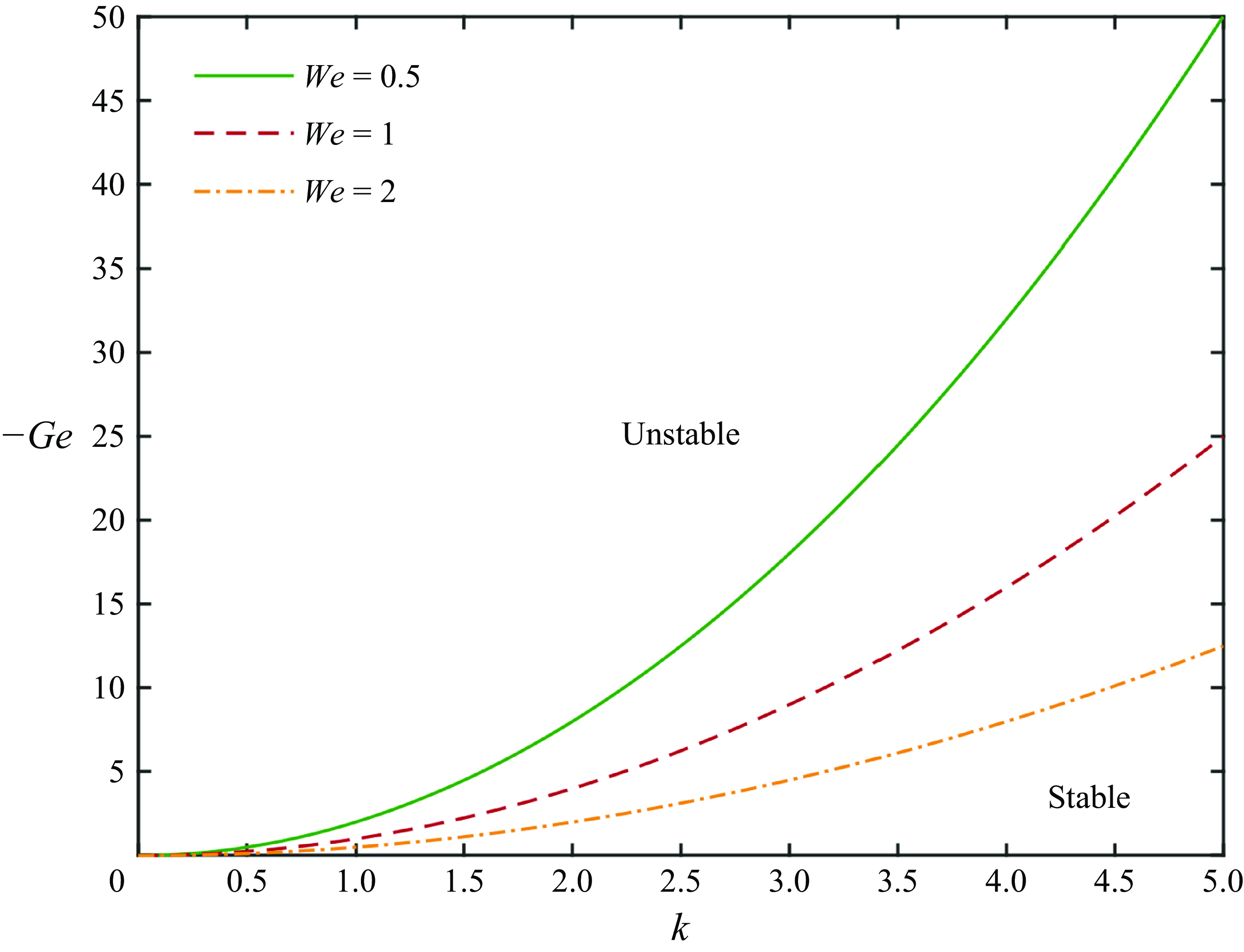
which is the condition for the neutral mode. We display the neutral curve as well as the stable and unstable regions in figure 2.

Figure 2.

The neutral curve of the linear stability analysis. The areas above and below the curve correspond to the unstable and stable regions, respectively.

It can be inferred from (3.8) and figure 2 that at moderate Re, unstable modes can occur only when Ge< 0. Conversely, when Ge $ \geqslant $ 0, the flow is linearly stable.

The linear stability of a shear liquid film on a horizontal plate has been studied by several authors. These works focus mainly on the cases where Ge = 0 (Smith & Davis Reference Smith and Davis1982) or Ge> 0 (Jurman & McCready Reference Jurman and McCready1989; Özgen, Degrez & Sarma Reference Özgen, Degrez and Sarma1998; Kadam, Patibandla & Roy Reference Kadam, Patibandla and Roy2023). The results suggest that the flow is linearly stable at moderate Re, and gravity is stabilising. This is consistent with the conclusions obtained in this paper.

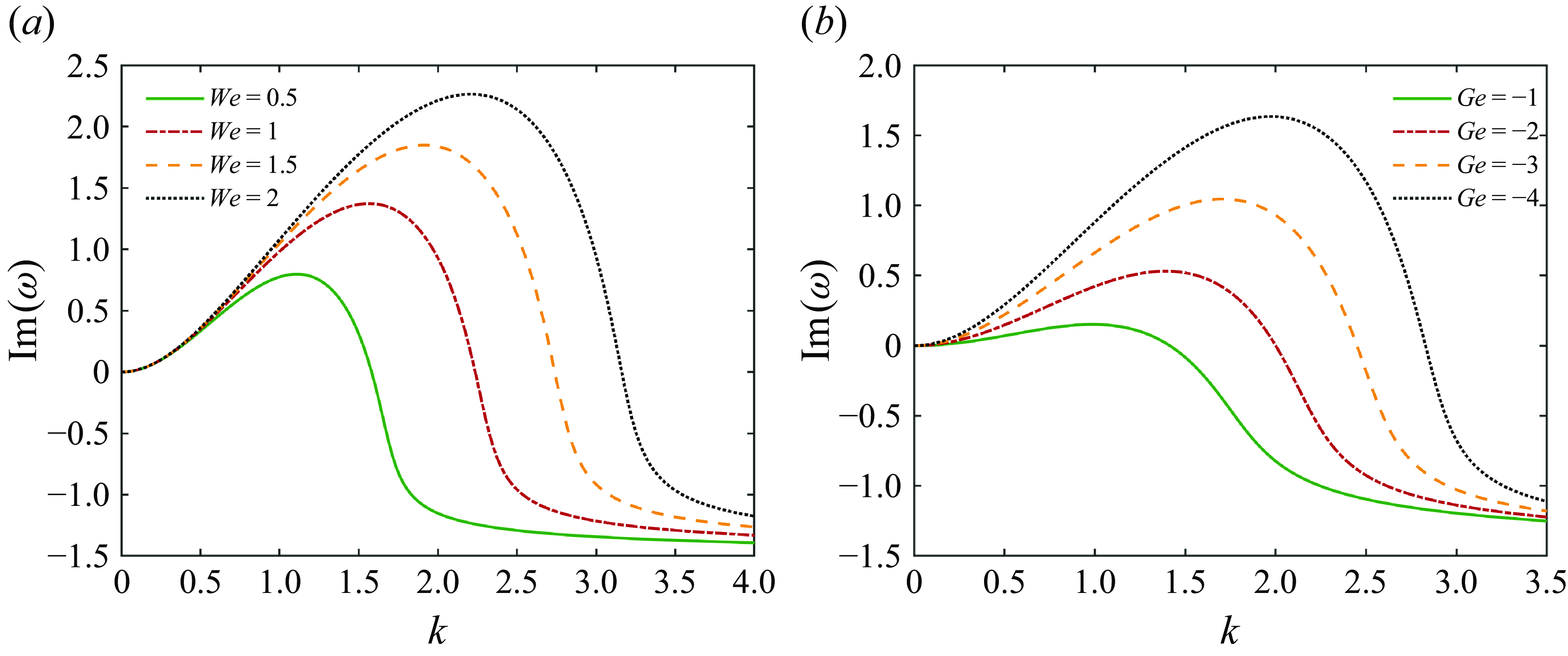
Then we study the dispersion curves of the perturbation growth rate $\mathrm{Im}(\omega )$ as a function of the wavenumber k. The dispersion curves at different parameters are displayed in figure 3. It can be found that the dispersion curves all pass through the origin $(0,0)$ . Subsequently, the growth rate first increases and then decreases with k, indicating the existence of a maximum growth rate. Additionally, when Ge decreases (increase of gravity) or We increases (decrease of surface tension), the growth rate also increases.

Figure 3.

The dispersion curves: (a) $\textit{Ge}=-5$ , (b) $\textit{We}=2$ .

3.2. Spatial-temporal mode

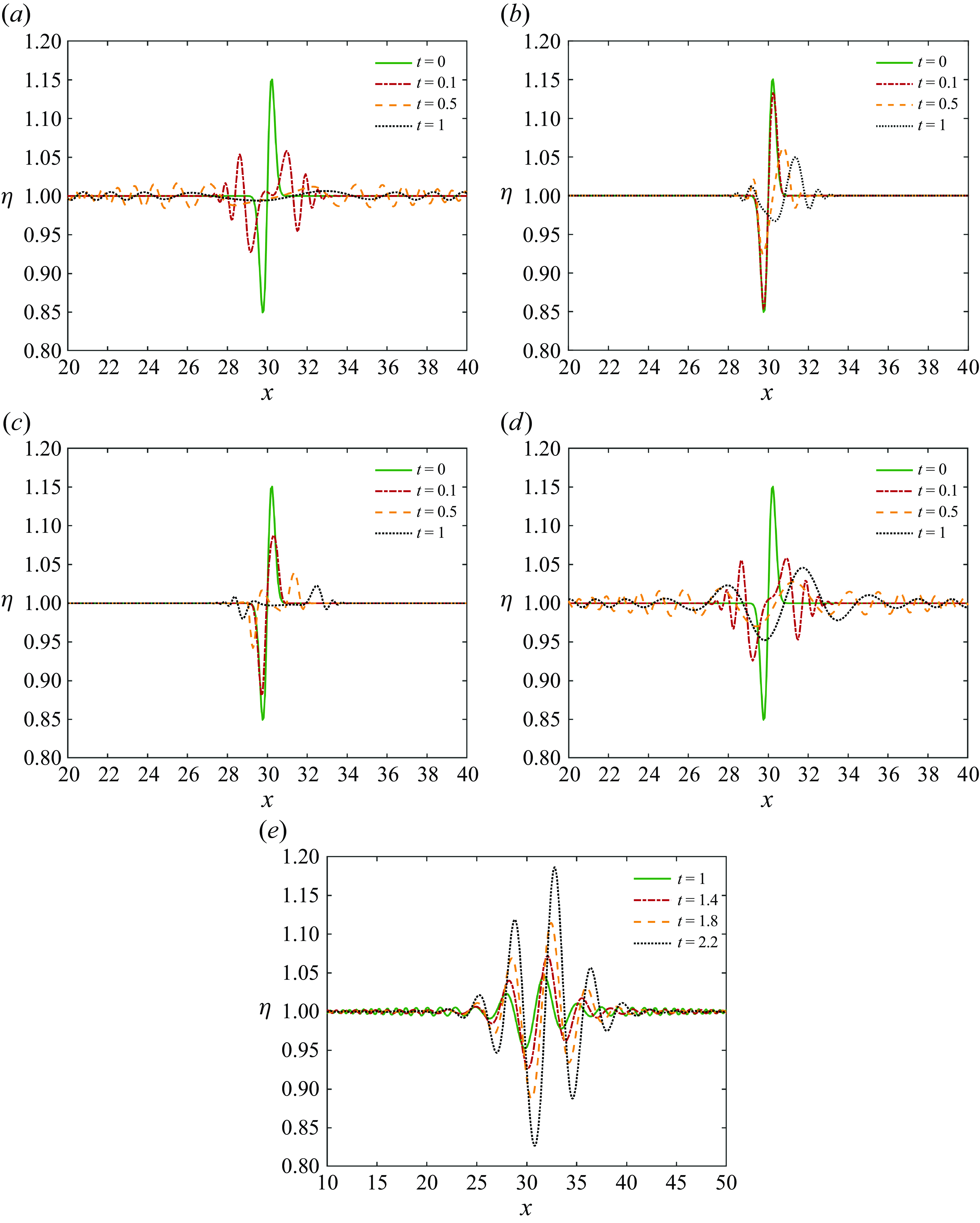
Many previous works on liquid films show that the disturbance waves can grow and spread (Kalliadasis et al. Reference Kalliadasis, Ruyer-Quil, Scheid and Velarde2011). Our numerical results in figure 4 also reveal that the wave amplitude varies over time, while the disturbances can propagate both upstream and downstream. In order to examine this property, the modal spatial-temporal analysis should be performed.

Figure 4.

The evolution of $\eta$ for a solitary wave at C = 1: (a) Ge = 0, We = 1; (b) Ge = 0, We = 100; (c) Ge = 2, We = 100; (d,e) $\textit{Ge}=-5$ , We = 1.

Vellingiri, Tseluiko & Kalliadasis (Reference Vellingiri, Tseluiko and Kalliadasis2015) considered the convective/absolute instability of a liquid film flowing down an inclined plate in the presence of a counter-current turbulent gas flow. The results show that at both low and high gas flow rates, the system exhibits convective instability, with the localised disturbances being convected downwards and upwards, respectively. When the gas flow rate is moderate, the instability becomes absolute, and localised disturbances spread across the whole domain.

Naraigh, Spelt & Shaw (Reference Náraigh, Spelt and Shaw2013) examined the convective/absolute instability in laminar and turbulent gas–liquid two-layer channel flow on a horizontal plate. The boundary between convective and absolute instability is determined. The regions of parameter space that produce absolute instability involve viscosity ratios of direct relevance to oil and gas flows.

In these two works, gravity is one of the driven forces for the flow (Vellingiri, Tseluiko & Kalliadasis Reference Vellingiri, Tseluiko and Kalliadasis2015), or stabilising as Ge> 0 (Naraigh, Spelt & Shaw Reference Náraigh, Spelt and Shaw2013). Here, we consider the instability for a suspended film, where Ge< 0.

In the spatial-temporal mode, both k and $\omega$ are complex. By differentiating both sides of (3.6) with respect to k simultaneously, the group velocity of disturbance can be obtained:

(3.9) \begin{equation} \frac{\mathrm{d}\omega }{\mathrm{d}k}=\frac{\dfrac{5}{4}\omega +2k\left(\textit{Ge}-\dfrac{1}{4}\right)+\dfrac{4}{\textit{We}}k^{3}+3\mathrm{i}}{2\omega -\dfrac{5}{4}k+3\mathrm{i}}. \end{equation}

Let $\mathrm{d}\omega /\mathrm{d}k=0$ . Then

(3.10) \begin{equation} \omega =-\frac{8}{5}k\left(\textit{Ge}-\frac{1}{4}\right)-\frac{16}{5\textit{We}}k^{3}-\frac{12}{5}\mathrm{i}. \end{equation}

Substituting (3.10) into (3.6), we can obtain the equation fork:

(3.11) \begin{align} \frac{256}{25\textit{We}^{2}}k^{6} &+ \frac{11+256\textit{Ge}}{25\textit{We}}k^{4}+\frac{144}{25\textit{We}}\mathrm{i}k^{3}+\frac{256\textit{Ge}^{2}-28\textit{Ge}-9}{100}k^{2}\nonumber \\ & +\frac{72\textit{Ge}-18}{25}\mathrm{i}k+\frac{36}{25}=0. \end{align}

Combining (3.10) and (3.11), $\omega$ can be determined. When its imaginary part is $\mathrm{Im}(\omega )=\omega _{i}\gt 0$ , the perturbation will grow exponentially with time at the point of excitation, which is an absolute instability. When $\omega _{i}\lt 0$ , the localised perturbation will be convected downwards, which is a convective instability. In addition, in absolute and convective instability, k corresponding to $\mathrm{d}\omega /\mathrm{d}k=0$ should be a pinch point in the complex k plane (Huerre & Rossi Reference Huerre, Rossi, Godreche and Manneville1998). Thus another condition should be satisfied: $\mathrm{d}^{2}\omega /\mathrm{d}k^{2}\neq 0$ .

By differentiating both sides of (3.9) with respect to k, and substituting $\mathrm{d}\omega /\mathrm{d}k=0$ , we derive

(3.12) \begin{equation} \frac{\mathrm{d}^{2}\omega }{\mathrm{d}k^{2}}=\frac{2\left(\textit{Ge}-\dfrac{1}{4}\right)+\dfrac{12}{\textit{We}}k^{2}}{2\omega -\dfrac{5}{4}k+3\mathrm{i}}. \end{equation}

For any parameters Ge, We, (3.11) has six complex roots for k. By substituting the numerically derived roots of (3.11) into (3.10) and (3.12), we find that at least one root makes $\omega _{i}\gt 0$ and $\mathrm{d}^{2}\omega /\mathrm{d}k^{2}\neq 0$ . So the instability is always an absolute instability. Thus we no longer need to show the absolute/convective instability regimes in the Ge–We plane.

4.1. Effects of Ge and We

First, we examine the effects of Ge and We on perturbations. In numerical calculations, the explicit difference scheme is used, where the temporal direction is first-order accurate, the spatial direction is fourth-order accurate, and the boundary conditions are second-order accurate (HDC). The size of the computational domain is $x\in [0,60]$ , the space step is ${\unicode[Arial]{x0394}} x=0.06$ and the time step is ${\unicode[Arial]{x0394}} t=10^{-7}$ .

The evolution of $\eta$ for a solitary wave is displayed in figure 4. The initial condition is

(4.1) \begin{equation} \eta | _{t=0}=1+0.58\exp (-10(x-30)^{2}) \boldsymbol{\cdot} \sin [2(x-30)] ,\quad q| _{t=0}=0.5. \end{equation}

When Ge = 0 (figure 4 a,b), the perturbation always decays over time. When We becomes larger, the attenuation speed slows down. This is because the surface tension is the main reason for suppressing the perturbation, and the increase in We corresponds to the decrease in the surface tension coefficient.

In figure 4(c), we find that the perturbation decays more rapidly at Ge> 0, while in figures 4(d) and 4(f), the perturbation starts to grow again after a period of attenuation at Ge< 0. Meanwhile, it can be seen that as time goes by, the oscillations generated by the perturbation continuously spread to the surrounding areas. However, at small Re, this propagation effect is far less obvious (figures 4 and 5 in HDC).

In order to study the effect of $q| _{t=0}$ on the evolution of $\eta$ , we choose the following initial conditions in figure 5:

(4.2) \begin{align} \eta | _{t=0} & = 1+0.58\exp (-10(x-30)^{2})^{\, \ast} \sin [2(x-30)] ,\nonumber \\ q| _{t=0} & = 0.5\pm 0.1\exp (-0.5(x-30)^{2})^ {\, \ast} \sin (2x-30). \end{align}

Here, the initial conditions of q in figures 5(a) and 5(b) are in the opposite phase. By comparing figure 4(a), figures 5(a) and 5(b), it can be found that the differences among the three are relatively small. So the evolution of $\eta$ is not very sensitive to $q| _{t=0}$ , and the influence of the latter is limited to a short initial period.

Figure 5.

The evolution of $\eta$ for a solitary wave at C = 1, Ge = 0, We = 1: (a)  $q| _{t=0}=0.5+ 0.1\exp (-0.5(x-30)^{2})^{\,*}\sin (2x-30)$ , (b)  $q| _{t=0}=0.5-0.1\exp (-0.5(x-30)^{2})^{\,*}\sin (2x-30)$ .

4.2. Steady travelling waves

The previous results suggest that surface tension will suppress the perturbation, while gravity will strengthen the perturbation at Ge< 0. Therefore, within a certain parameter range, the effects of the two may be comparable. Thus we can suppose that (2.26) has a steady-state solution at Ge< 0. Then ${\partial q}/{\partial t}={\partial \eta }/{\partial t} = 0$ , and (2.26a ) becomes

(4.3a) \begin{equation} q-C\eta =C_{1}, \end{equation}

where C ₁ is a constant. Substituting (4.3a ) into (2.26b ), we can obtain

(4.3b) \begin{align} \frac{\partial }{\partial x}\left[\left(\frac{1}{5}C^{2}+\frac{C_{1}}{20}\right)\eta +\frac{6{C_{1}}^{2}}{5\eta }+\frac{C}{20}\eta ^{2}+\frac{\eta ^{3}}{120}\right]&=\left(\frac{1}{\textit{We}}\frac{\partial ^{3}\eta }{\partial x^{3}}-\textit{Ge}\,\frac{\partial \eta }{\partial x}\right)\eta \nonumber \\ &\quad +\left[\frac{3}{2}-\frac{3\left(C\eta +C_{1}\right)}{\eta ^{2}}\right] \! . \end{align}

Solitary and periodic waves are discussed for (4.3b ) in the following.

4.2.1. Solitary waves

We consider the solitary wave in phase space coordinates $(\eta _{1},\eta _{2},\eta _{3})$ , where

(4.4) \begin{equation} \eta _{1}=\eta ,\quad \eta _{2}=\frac{\partial \eta }{\partial x},\quad \eta _{3}=\frac{\partial ^{2}\eta }{\partial x^{2}}. \end{equation}

Then we have

(4.5a,b) \begin{align}&\qquad\qquad\qquad\qquad\qquad\qquad\qquad \eta '_{1}=\eta _{2}, \quad \eta '_{2}=\eta _{3}, \\[-9pt] \nonumber \end{align}

(4.5c) \begin{align}& \eta '_{3}=\left\{\left[\left(\frac{1}{5}C^{2}+\frac{C_{1}}{20}\right)-\frac{6{C_{1}}^{2}}{5\eta _{1}^{2}}+\frac{C}{10}\eta _{1}+\frac{1}{40}\eta _{1}^{2}\right]\eta _{2}-3\left(\frac{1}{2}-\frac{C\eta _{1}+C_{1}}{\eta _{1}^{2}}\right)\right\}\frac{\textit{We}}{\eta _{1}}\nonumber \\& \qquad +{\textit{We}}\,\textit{Ge}\,\eta _{2}. \\[6pt] \nonumber \end{align}

Here, $\eta '_{i}$ indicates the derivative of $\eta _{i}$ with respect to x. When $x\rightarrow -\infty ,\ \eta \rightarrow \eta _{\infty },\ \eta ',\eta '''\rightarrow 0$ , it can be known from (2.26a ) that

(4.6) \begin{equation} q=\tfrac{1}{2}\eta _{\infty }^{2}, \quad \tfrac{1}{2}\eta _{\infty }^{2}-C\eta _{\infty }=C_{1}. \end{equation}

There are two stationary points $\mathrm{O}_{1}(\kappa _{1},0,0)$ and $\mathrm{O}_{2}(\kappa _{2},0,0)$ in the phase space, which have

(4.7) \begin{equation}\kappa _{1}=\eta _{\infty },\quad\kappa _{2}=2C-\eta _{\infty }.\end{equation}

Then we examine the linear stability of the stationary points:

(4.8) \begin{equation} \eta =\overline{\eta }+\widetilde{\eta }, \end{equation}

where $\overline{\eta }=\kappa _{1},\kappa _{2}$ , $\widetilde{\eta }=A\exp (\lambda x)$ , $A$ is a small amplitude, and $\lambda$ is the eigenvalue. Substituting (4.8) into (4.5), the eigenvalue equation of $\lambda$ can be derived. For $\mathrm{O}_{1}(\kappa _{1},0,0)$ ,

(4.9a) \begin{equation} \lambda ^{3}-\left[\frac{-C^{2}+5C\eta _{\infty }-\eta _{\infty }^{2}}{4\eta _{\infty }}+\textit{Ge}\right]{\textit{We}} \boldsymbol{\cdot} \lambda +\frac{3\textit{We}(\eta _{\infty }-C)}{\eta _{\infty }^{3}}=0, \end{equation}

and for $\mathrm{O}_{2}(\kappa _{2},0,0)$ ,

(4.9b) \begin{equation} \lambda ^{3}-\left[\frac{5C^{2}-C\eta _{\infty }-\eta _{\infty }^{2}}{4(2C-\eta _{\infty })}+\textit{Ge}\right]{\textit{We}} \boldsymbol{\cdot} \lambda -\frac{3\textit{We}(\eta _{\infty }-C)}{\left(2C-\eta _{\infty }\right)^{3}}=0. \end{equation}

When $2C-\eta _{\infty }\leqslant 0$ , there is only one stationary point. When $\eta _{\infty }=C$ , two stationary points overlap. In these two cases, no solitary waves are found.

When $C\gt ({1}/{2})\eta _{\infty },\ C\neq \eta _{\infty }$ , according to the root-finding formula, it can be known that both (4.9a ) and (4.9b ) have solutions with a real part greater than 0, suggesting that the liquid film is unstable. We obtain the trajectory in figure 6 by the numerical integration of (4.5), where the initial condition is chosen as a point near the stationary point O₁. Quasi-periodic oscillations occur between two stationary points O₁ and O₂ in figure 6(a), indicating the presence of heteroclinic trajectories. There are rapid oscillations for the heteroclinic trajectories in figure 6(b). The condition for the existence of the heteroclinic trajectories is $(-\textit{Ge})\in [Mi,Mx]$ , where Mi and Mx are the minimum and maximum allowable values of the parameter, respectively. If $(-\textit{Ge})\lt Mi$ or $(-\textit{Ge})\gt Mx$ , then the liquid film will rupture at a certain position ( $\eta \rightarrow 0$ ).

Figure 6.

The evolution of $\eta$ for heteroclinic trajectories between two stationary points: (a) $x\in (200,620)$ , (b) $x\in (240,370)$ . Here, $\eta _{\infty }=\kappa _{1}=2,\ \kappa _{2}=1,\ C=1.5$ , and We = 10, Ge = -2.

The computation suggests that the specific region of Ge depends on the initial disturbance, while the approximate range is displayed in figure 7. It can be found that both Mx and Mi decrease with the increase of We, while the variations of Mx and Mi with C are non-monotonic.

Figure 7.

The approximate range of Ge when there exist heteroclinic trajectories between the two stationary points. Here, $\eta _{\infty }=\kappa _{1}=2$ .

4.2.2. Periodic waves

For periodic waves, the evolution of $\eta$ is examined by the numerical simulation. The results show that the shapes of the steady-state periodic waves under different parameters can be divided into five types. The corresponding parameter range depends on the initial perturbation. In the following, we take $\eta | _{t=0}=1+0.15 \boldsymbol{\cdot} \sin x ,\ q| _{t=0}=0.5$ as the initial conditions and draw five types of perturbation waves. In the following calculations, we present the results in a stationary reference frame, where C = 0. The waves propagate along the positive x-axis, and the wave speeds $V_w$ are shown in figures 8–12.

Figure 8.

The evolution of $\eta$ for a periodic wave at C = 0, We = 2: (a) $\textit{Ge}=-0.5$ , (b) $\textit{Ge}=-0.6$ , (c) $\textit{Ge}=-0.7$ . The wave speeds of these waves are $V_w$ = 1.05, 0.97 and 0.90, respectively.

The first wave speed is displayed in figure 8 at We = 2, where the perturbation wave tends to exhibit a sine-function-like behaviour. In figure 8(a) ( $\textit{Ge}=-0.5$ ), the perturbation wave will decay over time, while in figure 8(b) ( $\textit{Ge}=-0.6$ ) and figure 8(c) ( $\textit{Ge}=-0.7$ ), the perturbation wave can reach a steady state after a certain period of time. This indicates that there can be multiple Ge values in equilibrium with We. In addition, the amplitude of the steady-state perturbation wave increases with the decrease of Ge.

Figure 9.

The evolution of $\eta$ for a periodic wave at C = 0, $\textit{Ge}=-1.4$ and We = 2. The wave speed is $V_w$ = 0.90.

Figure 10.

The evolution of $\eta$ for a periodic wave at C = 0, $\textit{Ge}=-0.05$ and We = 60. The wave speed is $V_w$ = 1.05.

Figure 11.

The evolution of $\eta$ for a periodic wave at C = 0, $\textit{Ge}=-0.07$ and We = 60. The wave speed is $V_w$ = 0.97.

Figure 12.

The evolution of $\eta$ for a periodic wave at C = 0, $\textit{Ge}=-0.11$ and We = 60. The wave speed is $V_w$ = 0.97.

Further calculations show that when We is small (We ∼ O(1)), if Ge takes an appropriate value, then the perturbation wave will present the above-mentioned sine function pattern. When Ge is appropriately reduced, the perturbation will change into the second pattern, as shown in figure 9, where $\textit{Ge}=-1.4$ and We = 2.

It can be seen from figure 9 that when the perturbation wave reaches steady state, the maximum and minimum values of $\eta$ are $\eta _{\textit{max}}\approx 2.3$ and $\eta _{\textit{min}}\approx 0.3$ , respectively. The troughs of the waves are relatively flat, while the perturbation amplitude increases significantly compared with that at the initial moment. This is because the decrease in Ge corresponds to the increase in gravity, which makes the perturbation more unstable. Further decreasing Ge will make the amplitude continue to grow and eventually lead to the rupture of the liquid film.

Frank (Reference Frank2006) numerically investigated nonlinear periodic 2-D waves on a liquid film driven by laminar flow of a gas. The wave pattern at Re = 13.8 and $\varpi =d/l\sim 0.03$ in figure 2 of this work is similar to that in figure 9. However, more than one capillary ripple can be seen in figure 2 of Frank (Reference Frank2006), while this is not the case here. The difference might be due to the fact that gravity was not considered in the former, whereas in this study, gravity is a significant factor contributing to the instability. This results in the capillary ripples being less pronounced.

When We is relatively large (We > O(1)), another three types of perturbation waves are detected. Figure 10 shows the evolution of $\eta$ for a periodic wave at C = 0, $\textit{Ge}=-0.05$ and We = 60. It can be found that the amplitude of the steady-state wave is significantly reduced compared with that of the initial state. In addition, the length of the rising section (from the trough to the peak) is significantly greater than that of the descending section, which are the main features distinguishing it from the sine function wave in figure 8.

When Ge decreases slightly, the perturbation can change into the pattern displayed in figure 11, where $\textit{Ge}=-0.07$ and We = 60. The amplitude in its steady state is obviously larger than that shown in figure 10. There are significant fluctuations in the rising section from the trough to the peak.

When Ge continues to decrease, we find the fifth type of wave pattern, displayed in figure 12, where $\textit{Ge}=-0.11$ and We = 60. Although the wave pattern is also similar to the sine function, its wavenumber has changed from 1 at the initial moment to 2 in the steady state. In contrast, for all the perturbation waves in figures 8–11, the wavenumber in the steady state is 1, which is the same as that at the initial moment. This shows that gravity can increase not only the wave amplitude but also the wavenumber.

In addition, the capillary ripples disappear in figure 12. This can be explained as follows. When We increases, the ratio of gravity to surface tension becomes larger, leading to an increase in the amplitude of capillary ripples that were originally suppressed by surface tension, thereby increasing the wavenumber. When We is increased further, the system may becomes chaotic (see figure 19 below), and there are also no capillary ripples.

4.3. Quasi-periodic and chaotic solutions

In addition, within some parameter ranges, we find that $\eta$ shows no sign of tending towards a steady state even after a long period of time. It can be found in figure 13(a) that the amplitude of the perturbation wave seems to decrease with the increase of time. However, figure 13(b) shows that after a sufficiently long time, the perturbation does not decay. The wave patterns at different moments all have significant differences. Some waves have two peaks and two troughs, while others have only one peak or one trough. Moreover, the amplitudes of their peaks and troughs are also different.

Figure 13.

The evolution of $\eta$ for a periodic wave at C = 0, $\textit{Ge}=-0.1$ and We = 60: (a) $t=0{-}2700$ , (b) $t=2700{-}5400$ .

In order to study these evolution characteristics, we use (4.4) and display the variation of $\eta ,\ {\partial \eta }/{\partial x},\ {\partial ^{2}\eta }/{\partial x^{2}}$ at x = 0 with time in the phase space coordinates $(\eta _{1},\eta _{2},\eta _{3})$ . The attractor of the evolution is displayed in figure 14, showing a strange shape. This easily reminds us of the strange attractor in the Lorenz system. However, at this time, it is still difficult to judge whether this solution is chaotic or not.

Figure 14.

The attractor in the phase space for a periodic wave at C = 0, $\textit{Ge}=-0.1$ and We = 60: (a) 3-D view; (b) $\eta _{1},\eta _{2}$ section; (c) $\eta _{2},\eta _{3}$ section; (d) $\eta _{1},\eta _{3}$ section. The initial conditions are $\left.\eta \right| _{t=0}=1+0.15 \boldsymbol{\cdot} \sin x$ and $q| _{t=0}=0.5$ .

Therefore, we display the Poincaré section of the attractor in figure 15, where $\eta _{1}=1$ . It can be seen that although the orbits of the attractor are very dense in figure 14, most points on the Poincaré section are located in several lines. However, in a chaotic system, the points on the Poincaré section usually present a complex and random distribution, which covers a large area. Based on this property, we believe that the system in figure 14 has not reached chaos, and classify it as a quasi-periodic solution.

Figure 15.

The Poincaré section ( $\eta _{1}=1$ ) of the attractor in figure 14.

Then we examine the dependence of evolution on initial conditions. Figure 16 shows the evolutions of $\eta$ at two close initial conditions. It can be found that after a long period of time, the difference between the two is still very small. This further indicates that the system has not reached chaos.

Figure 16.

The evolutions of $\eta$ at x = 0 for a periodic wave at different initial conditions: (a) $\left.\eta \right| _{t=0}=1+0.15 \boldsymbol{\cdot} \sin x$ , (b) $\eta | _{t=0}=1+0.15 \boldsymbol{\cdot} \sin x+0.01 \boldsymbol{\cdot} \sin 5x$ . Other conditions and parameters are $q| _{t=0}=0.5$ , C = 0, $\textit{Ge}=-0.1$ and We = 60.

However, we find chaotic evolutions at other parameters and initial conditions. Figure 17 shows the attractor in the phase space with the parameters $\textit{Ge}=-0.11$ , We = 100 and initial conditions $\eta | _{t=0}=1+0.3 \boldsymbol{\cdot} \sin x ,\ q| _{t=0}=0.5$ . Its Poincaré section is displayed in figure 18. It can be found that although the shape of the attractor in figure 17 is similar to that in figure 14, there are significant differences between their Poincaré sections. In figure 18, dense points are distributed in a very wide area, which is a remarkable feature of chaos.

Figure 17.

The attractor in the phase space for a periodic wave at C = 0, $\textit{Ge}=-0.11$ and We = 100. The initial conditions are $\eta | _{t=0}=1+0.3 \boldsymbol{\cdot} \sin x$ and $q| _{t=0}=0.5$ .

Figure 18.

The Poincaré section ( $\eta _{1}=1$ ) of the attractor in figure 17.

Figure 19.

The evolutions of $\eta$ at x = 0 for a periodic wave at different initial conditions: (a) $\left.\eta \right| _{t=0}=1+0.3 \boldsymbol{\cdot} \sin x$ , (b) $\left.\eta \right| _{t=0}=1+0.3 \boldsymbol{\cdot} \sin x + 0.01 \boldsymbol{\cdot} \sin 5x$ . Other conditions and parameters are $q| _{t=0}=0.5$ , C = 0, $\textit{Ge}=-0.11$ and We = 100.

Similarly, we would like to check the sensitivity of the evolution to initial conditions for the system in figure 17. In figure 19, we compare the evolutions of $\eta$ at two close initial conditions. The results suggests that after a period of time, the evolutions of the two systems have become completely different, indicating that the system is in a chaotic state.

It should be pointed out that the chaotic state in figure 17 is a spatial-temporal chaos governed by the partial differential equations in (2.26), and figure 17 shows only the attractor at x = 0. For comparison, some chaotic systems in phase space are governed by ordinary differential equations, such as the homoclinic chaos (Kalliadasis et al. Reference Kalliadasis, Ruyer-Quil, Scheid and Velarde2011, p. 223) and the strange attractor of Lorenz equations (Strogatz Reference Strogatz2015). Therefore, the complexity of the former is much greater than that of the latter two.

Figures 14–19 display the evolution at x = 0. In order to examine the evolutions at other positions, we plot the attractors and the Poincaré sections at $x=2\pi /3$ and $x=4\pi /3$ in figures 20 and 21, respectively. The results show that they are similar to those at x = 0 in figures 14 and 15.

Figure 20.

The evolutions of $\eta$ for a periodic wave at (a) $x=2\pi /3$ , (b) $x=4\pi /3$ . Other conditions and parameters are the same as those in figure 14.

Figure 21.

The Poincaré sections ( $\eta _{1}=1$ ) of the attractors in figure 20: (a) $x=2\pi /3$ , (b) $x=4\pi /3$ .

Figure 22.

The parameter ranges corresponding to different wave patterns at the initial condition $\left.\eta \right| _{t=0}=1 + 0.15 \boldsymbol{\cdot} \sin x$ . Here, types 1–7 correspond to the wave patterns in figures 8– 13 and 17, respectively.

4.4. Parameter ranges of wave patterns

We have demonstrated the various patterns that periodic waves can make under different parameters. Here, we present the parameter ranges corresponding to these patterns in figure 22. When (–Ge) is small, surface waves gradually decay over time, whereas when (–Ge) is sufficiently large, the amplitude of surface waves continuously increases until the film eventually breaks. Between these two regimes, the system admits steady travelling wave solutions (types 1–5) or solutions that neither decay nor diverge (types 6 and 7). Here, types 1–7 correspond to the patterns in figures 8–13 and 17, respectively. As We increases, the wave pattern undergoes successive bifurcations, giving rise to many new types. Additionally, if the initial conditions are modified as $\left.\eta \right| _{t=0}=1+0.3 \boldsymbol{\cdot} \sin x$ , then the boundaries between different regions in the figure 22 will shift slightly, but the overall shapes of the regions remain largely unchanged.