Aims

The idea of measuring living standards by means of ‘outputs’ (consumption and expenditure) rather than ‘inputs’ (income and wealth) is increasingly influential among academics and policy-makers. There is a particular interest in using ‘deprivation indicators’ to investigate living standards at the lower end of the scale. This idea goes back at least to Townsend's monumental study of Poverty in the United Kingdom (1979). A more recent study of Poverty and Social Exclusion in Britain (Gordon et al., Reference Gordon, Adelman, Ashworth, Bradshaw, Levitas, Middleton, Pantazis, Patsios, Payne, Townsend and Williams2000; Pantazis et al., Reference Pantazis, Gordon and Levitas2006) aimed to take the approach to its logical conclusion – though for a sceptical view see McKay (Reference McKay2004). Although most analyses of deprivation indicators have been undertaken by researchers specialising in social policy, others approaching the data from an economist's perspective include Desai and Shah (Reference Desai and Shah1988) and Cappellari and Jenkins (Reference Cappellari and Jenkins2006). The European Union is placing increasing emphasis on the use of indicators to monitor social conditions (Guio, Reference Guio2005; Marlier et al., Reference Marlier, Atkinson, Cantillon and Nolan2007); and the UK government now includes deprivation indicators among its suite of measures to monitor progress towards the abolition of child poverty (DWP, 2003, 2008; Willitts, Reference Willitts2006).

Given the alternative approaches to assessing living standards, it is increasingly important to analyse the relationship between deprivation indicators and income, and to discuss the implications of that relationship for our understanding of poverty. In particular, most of the analyses to date have been of cross-sectional data. A series of articles by Whelan et al. (for example, Reference Whelan, Layte and Maitre2003, Reference Whelan, Layte and Maitre2004) has shown that households in persistent poverty report more material deprivation than those in transitory poverty, but as far as we know this paper is the first systematic analysis of the joint changes in deprivation and income from year to year.

This paper uses nine consecutive years of a household panel survey to show what happens to deprivation scores when people's incomes go up or down. To motivate the research questions, the next section is a preamble to the main analysis, briefly discussing theoretical issues around the interpretation of deprivation indicators. The main research questions about the relationship between income and deprivation over time follow. We then describe the data, focusing especially on the measures of income and of deprivation. The empirical content starts with a cross-sectional analysis, replicating the approach adopted in previous studies, and then uses a longitudinal analysis to distinguish between what we call the ‘underlying’ and ‘dynamic’ effects of low income (operationalised as between and within cases effects). The final section discusses conclusions both for poverty measurement and for policy.

Interpreting deprivation indicators

A formal definition of poverty was adopted by the European Union in 1984:

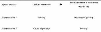
The EU definition does not make clear which of the two problems – ‘limited resources’ or ‘exclusion from the minimum way of life’ – constitutes the essence of ‘poverty’ (Figure 1). One view could be that poverty consists of a lack of resources (one of whose main symptoms is exclusion from a minimum way of life). Another view could be that poverty consists of social exclusion (one of whose main causes is lack of resources).

Figure 1.

Two interpretations of the essence of poverty

Townsend (Reference Townsend1979) adopted the former approach. He used a multi-item deprivation index to study the relationship between income and deprivation, looking for evidence that there was a boundary line in the income distribution below which living standards plunged to unacceptably low levels. He and many successors used deprivation indicators to demonstrate in one way or another that low income is a bad thing, and should be labelled ‘poverty’.

The contrasting perspective is that deprivation is a bad thing. Ringen (Reference Ringen1988) argued that a low income was only an indirect measure of poverty, and that direct measures of social exclusion were required. A second school of researchers has used deprivation indicators to define poverty and count the poor (Mack and Lansley, Reference Mack and Lansley1985; Gordon et al., Reference Gordon, Adelman, Ashworth, Bradshaw, Levitas, Middleton, Pantazis, Patsios, Payne, Townsend and Williams2000; Pantazis et al., Reference Pantazis, Gordon and Levitas2006). Several researchers have noted that those on low income and those with high deprivation scores are not necessarily the same people (Nolan and Whelan, Reference Nolan and Whelan1996; Whelan et al., Reference Whelan, Layte and Maitre2004). One interpretation has been that income is a weak predictor of poverty.

While arguments about what ‘poverty’ consists of may seem theoretical, or even merely linguistic, there are important empirical implications. The use of an index of material deprivation as just an indicator, to identify groups at risk of poverty or to calibrate a poverty line, can be based on a fairly weak set of assumptions. The principal requirement is that the items in the index should collectively reflect basic living standards, and be appropriately sensitive to income variations at the lower end of the scale. The indicator's job is to tell us about the different experiences of households analysed by income, family composition, age and so on.

In contrast, using an index as an actual measure of poverty requires a very strong set of assumptions. The index should sample the whole range of areas of consumption (including those where no deprivation is in fact experienced, and others where deprivation is not associated with low income), in order to obtain a balanced measure of output inequality. A concept of secondary poverty may be required (as originally proposed by Seebohm Rowntree in 1901) to account for people whose high deprivation score is not associated with low income, and is presumably caused by ‘wasteful’ spending.

We argue that no index can support the strong set of assumptions required to treat it as a direct measure of poverty. This article is based on the weak set of assumptions required to treat an index of deprivation as just an indicator of living standards. The tool makes a more valuable contribution to research and policy if it is not burdened with too heavy a responsibility.

We have stylised this debate as two opposing schools of thought, in order to focus on some important measurement issues which require careful consideration. In practice, many analysts use low income and high deprivation scores as complements, rather than as alternatives. A compromise is to define the poor as households who combine low income with high deprivation scores (Nolan and Whelan, Reference Nolan and Whelan1996; DWP, 2003). The main focus in this article is on the relationship between the two, especially over time.

Research questions

The dynamics of low income have been much discussed since the Panel Study on Income Dynamics (PSID) first provided panel data in the US in the 1970s (Bane and Ellwood, Reference Bane and Ellwood1994), followed in Britain by the British Household Panel Study (BHPS) in the 1990s (Jenkins and Rigg, Reference Jenkins and Rigg2001; Devicienti, Reference Devicienti2001). A rigorous analysis of deprivation requires a dynamic approach too. Our research questions are not concerned with deprivation taken on its own, but on the links between deprivation and income (and other household characteristics) over time.

The key questions are:

• • Given (as we confirm) that households with low incomes in any year tend to report high deprivation scores in the same year, does a household's deprivation systematically rise when its income falls (and vice versa) from year to year?

• • Or is the cross-sectional association based on long-term similarities in households’ positions on the two dimensions, with each fluctuating from year to year independently of the other?

• • Are the effects of income on deprivation confounded by other predictor variables, such as family structure, ill health, housing or employment characteristics?

• • The relationship between income and deprivation is usually interpreted as a causal one (low income makes people deprived). Does the dynamic relationship identified in the data support causal inferences?

• • Is there evidence that people smooth their living standards across short periods of unusually low or high income (Brewer et al., Reference Brewer, Goodman and Leicester2006)?

• • Is there evidence that changes in deprivation respond to changes in income over a period of years, rather than immediately – a lagged effect?

• • What does the analysis tell us about the relative severity of spells of persistent, recurrent or temporary poverty?

• • What are the conclusions for poverty measurement, and for policy?

Income and deprivation measures in the British Household Panel Survey sample

The BHPS is based on a random sample of about 5,500 households originally selected in 1991. All adult members of those households, plus their children as they have reached the age of 16, have been interviewed each year since then. The analysis here uses the nine years between 1996 and 2004: wave 6 through to wave 14. The analysis is confined to the original Great Britain sample, and does not include the booster samples added later in Scotland, Wales and Northern Ireland.

A parallel analysis of BHPS deprivation data among older people by members of the same research team (Berthoud et al., Reference Berthoud, Blekesaune and Hancock2006, Reference Berthoud, Blekesaune and Hancock2009) showed that in that group the construction of deprivation indices is highly sensitive to respondents’ subjective interpretations. It also identified distinct ageing and cohort effects among the pensioner population. The issues addressed in the current paper are in some ways more straightforward, and it would have been difficult to address both sets of research questions at the same time. So the analysis here is confined to respondents (including children) below pensionable age (60 for women, 65 for men).

The sample analysed is confined to those who took part on at least five occasions (and whose household reported complete income and deprivation data on each of those occasions). All the variables analysed are defined for whole households, so that all household members share the same position in each year. Benchmarks (such as median, mean, standard deviation, centiles) of the distributions of income and of deprivation, used to define variables, are derived from an analysis at the household level, covering all age groups. But the unit at the analysis stage is the individual (within the non-pensioner age range), because only individuals can be followed from year to year through potential changes of household membership.Footnote ¹

Calculations of robust standard errors are based on treating the household from which the respondent was originally sampled in 1991 as the ‘cluster’: this technique usefully compensates both for the common outcome within each household in any wave, and for the association across waves for each individual.

The sample analysed consists of 6,590 individuals from 2,279 original households, providing 50,159 person-wave observations.

Deprivation index

The deprivation score was compiled with reference to three principles.

• • There should be a fairly large number of items contributing to the index, rather than require the analysis to lean too heavily on one indicator which might behave idiosyncratically.

• • The candidate items should be correlated with each other, indicating the existence of a common underlying construct (which we label deprivation).

• • Each of the items, and the index as a whole, should be correlated with (low) income.

No doubt other analysts would have defined an index slightly differently, and there is no suggestion that the chosen index is ideal, or that such an ideal exists (in the sense that one might conceive of, though possibly not achieve, an ideal measure of household income). It is one of a potentially large family of deprivation indicators, all of which should yield approximately the same results if the approach has any validity.

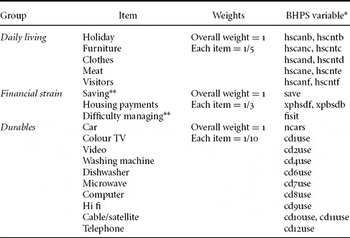
The index was compiled from 18 question items organised in three groups, as recorded in Table 1. Each item and group were initially scored between 0 and 1 as follows:

• Daily living: 0.5 for each item the household did not have; 1.0 for each item they said they could not afford.Footnote ²

• Financial strain: equal-interval scores ranging from 0 for best possible answer to 1 for worst possible

• Durables: –1 for each item possessed.Footnote ³

TABLE 1.

Components of the BHPS deprivation index

Notes: *Full wording of the questions can be checked by looking up the BHPS variable names at www.iser.essex.ac.uk/ulsc/bhps.

**These two questions were asked of every member of each household. The index is based on the answers by the conventionally defined ‘head of household’. All the other questions were asked of one member of the household on behalf of all.

The raw scores for each of the 18 items were then standardised (Z scores) to have a mean of 0 and a standard deviation equal to the weight assigned to the item in the overall index (see third column of Table 1). This meant that when the sub-scores were averaged within each household, each of the three groups contributed approximately the same variance to the total (to avoid giving undue weight to the group which happened to have the largest number of questions). The resulting overall index had a Chronbach's α of 0.75.Footnote ⁴

The steps described so far are appropriate for deriving an index based on data referring to one point in time. The present study required consideration of an issue not relevant to previous cross-sectional studies: the validity of an index over time. What happens if the average score consistently rises or falls over the years? This is crucial both for a dynamic analysis, and for time-series such as measuring the reduction in child poverty.

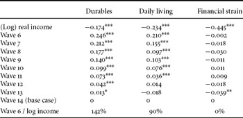
The three groups within the overall index had very different patterns of variation over time. Table 2 presents regressions showing the evolution over time of the deprivation score for each group of items, controlling for the log of real (absolute) income.

TABLE 2.

Wave on wave trends in the average score on each group of deprivation items (regression coefficients)

Notes: Both deprivation and income are measured absolutely in this table. Subsequent analysis expresses each relative to the wave average. Additional controls for household structure, age, health, education, income sources, housing tenure and region, as shown in Table 3, were included but not reported in this table. *** = significant at 99.9 per cent level; ** at 99 per cent level; * at 95 per cent level.

As one would have expected, the ownership of consumer durables – including many electronic gadgets that have been invented quite recently – has been spreading rapidly – so deprivation measured as lack of consumer durables has been reducing. This apparent reduction is explained in part by rising income, but the year-on-year ‘improvement’ is visible even after that has been taken into account.

One would not have expected a trend over time in households’ access to the basics of daily living represented by the items labelled ‘meat’ to ‘friends round’. These were intended by the questions’ authors to have some absolute validity as indicators of restricted living standards. But it turns out that there has also been a steady reduction in deprivation measured by the daily living questions – part of it accounted for by rising average incomes, and a larger part of it running ahead of income growth. The trend is not as strong as it was for durables deprivation, but nevertheless significant.

There was a slight reduction in deprivation measured as financial strain over the period analysed, but the trend was insignificant once rising incomes had been allowed for.

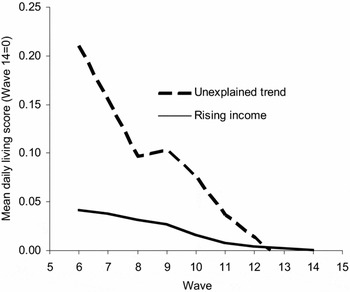
Figure 2 illustrates the wave-on-wave changes in daily living deprivation scores. This element of the overall index is important both because the down-trend could not have been predicted, and also because it is most similar to the deprivation index based on the Family Resources Survey used by the government for its monitoring of child poverty. There has indeed been a reduction in daily living deprivation, attributable to rising incomes, but there has been a much larger fall in average scores, which cannot be explained by changes in income or any of the other covariates included in the model.Footnote ⁵

Figure 2.

Trends in daily living deprivation score: reduction attributable to changing incomes compared with unexplained reduction

The sharp unexplained reduction in the level of deprivation, as measured by daily living, is surprising; so much so that many analysts have interpreted the apparent improvement in living standards as the result of rising incomes (McKay and Collard, Reference McKay and Collard2004; Willitts, Reference Willitts2006). Very similar trends have been observed in the Families and Children Survey, and in 13 out of 14 countries covered by the European Community Household Panel survey.Footnote ⁶

So the deprivation scores analysed in the remainder of this paper are relative to annual averages. This was achieved by undertaking the standardisation of each input variable (Z scores, see above) separately for each BHPS wave.

Cross-sectional relationships

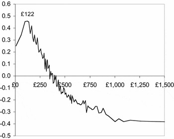
The objective of the research was to analyse the relationship between income and deprivation in detail. Figure 3 is designed to show whether this relationship is consistent across the whole of the income distribution. Households have been divided into centile groups according to their position in each wave's income distribution. Each group is plotted according to its mean weekly income, using the values from the Wave 14 distribution (x-axis) and mean relative deprivation score (y-axis).

Figure 3.

Deprivation score plotted by income: pooled wave-specific centile groups of the income distribution.

Note: The x-axis is presented in pounds per week of the wave 14 income distribution.

The graph shows a very consistent relationship between high income and low deprivation, above the third percentile. The downwards slope of the graph over most its course is exactly what would have been expected on the assumption that low income is associated with low living standards (high deprivation scores). The shape of the curve (steep to start with and becoming shallower) is consistent with the view that lower levels of deprivation are most closely associated with a proportionate, rather than an absolute, increase in income. This curve is captured in the following analysis by using the log of income as the main predictor variable.

But the bottom three centile groups – below £122 per week at 2005 rates – were less deprived than would have been expected, given their reported incomes. This twist in the tail of the income distribution has been noted before in many analyses of the relation between income and outcomes (see Elam et al., Reference Elam, Lee and Tadd1999; Berthoud et al., Reference Berthoud, Bryan and Bardasi2004; Brewer et al., Reference Brewer, Goodman and Leicester2006, Reference Brewer, O'Dea, Paull and Sibieta2009).

The inconsistency in the apparent relationship between very low income and various outcome measures gives rise to the suspicion that some of the very low incomes are under-reported. There are two ways of dealing with it in more detailed analysis. One is to include all incomes in the regression models, but with an explicit term to represent the deviant behaviour of very low incomes. The other is to omit very low incomes from the analysis altogether, on the assumption that measurement error is distorting the estimates of the true relationships. In the remainder of this paper, we adopt the latter approach, as it provides a much clearer picture, especially for readers who may not be very familiar with statistical techniques.Footnote ⁷

All following analysis in the main paper is therefore confined to households whose reported income (in the year analysed) was above the third percentile

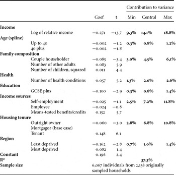
Table 3 presents a straightforward cross-sectional regression model, explaining variations between households’ deprivation scores in terms of their incomes and other predictor variables. The equation is estimated by ordinary least squares (OLS), using Wave 10 (the middle of the available sequence, and so broadly representative of the period analysed). The subsequent longitudinal analysis is more important to the conclusions of this paper, but the initial cross-sectional version serves two purposes: to replicate the approach used by previous, and probable future, analysts of snapshot deprivation scores; and to use a simple model to introduce the variables and the outputs from the equation before moving on to the more complex longitudinal versions.

TABLE 3.

Cross-sectional regressions predicting relative deprivation score in wave 10 (ordinary least squares, originally sampled households treated as clusters)

The results are presented in Table 3.

• Income. As explained, each household's total income was calculated as a percentage of the national median for the wave in question, and expressed as a logarithm. Relative deprivation falls with increasing income, and especially over the lower ranges of the distribution (for given absolute increases in income).

• Age. Age (based on the oldest member of the household) was included in the analysis in two sequences – up to 40 and above 40.Footnote ⁸ Neither was significant. Remember that pensioners, who are known to have low deprivation scores in relation to their income, are not included in this analysis.

• Family composition. Where the conventionally defined head of household was a member of a couple, deprivation scores were lower. This result contradicts most equivalence scales (which assume that additional people raise costs and lower living standards), but the same relationship has been observed in several other studies (see Berthoud and Ford, Reference Berthoud and Ford1996). However, additional adults other than the partner of the householder increase deprivation. The majority of such additional adults are the offspring of the householder, no longer of dependent age. Families with dependent children tend to have higher deprivation scores, controlling for income. The effect is stronger for larger numbers of children. (A linear term in number of children was not significant when combined with the quadratic term.)

• Health. Ill health and disability are known to add to household expenditure needs, and previous studies (Zaidi and Burchardt, Reference Zaidi and Burchardt2005) have shown that they are associated with higher deprivation scores. The analysis here counts the total number of ill-health conditions reported by any member of the household – if more than one member, then the one with the most conditions. Worse health measured in this way means more deprivation.

• Education. Households containing at least one person with qualifications to O/GCSE level or above were significantly less deprived than less-educated households, after taking account of other factors, including income.

• Income sources. Households containing one or more worker, self-employed or an employee, appeared to have lower deprivation scores than expected, given their other characteristics, but these coefficients were not significant. If the household reported receipt of any means-tested benefits or tax credits (apart from child credit), then it was more deprived, even after taking account of the low incomes available to such families.

• Housing tenure. Outright owners were less deprived than households still paying a mortgage. Those who rented their homes were more deprived. It might be thought that these variations could be explained by the housing costs faced by each tenure type, but the effects were only slightly reduced if a direct measure of housing costs was added to the model.

• Region. Among 18 regions and conurbations, coefficients ranged from –0.162 (less deprived than expected) in Merseyside to +0.082 (more than expected) in Inner London – both compared with the largest region, the Rest of the South East, treated as the base case. These regional variations were collectively significant, but to save space are not shown in detail in the tables.

The variables in Table 3 explained 37 per cent of the variance in the dependent variable (R²). The right-hand side of the table decomposes this explanatory power across the groups of variables.Footnote ⁹

According to this analysis, income is easily the most powerful predictor of deprivation scores, accounting for about two-fifths of the overall explanation of variance. But income sources and housing tenure are also important contributors, although the wide range of variance–share estimates for these two groups suggests that these variables overlap with others (especially income itself). Household composition and health also contribute to the variance, but these two well-established indicators of objective need seem to be less important than the institutional relationships captured by tenure and income sources.

Of course, this cross-sectional analysis – comparing households’ deprivation scores, income, household composition and so on all at the same point in time – describes the position in the sense of showing who is most likely to be deprived. It does not explain the process in the sense of showing how they come to be deprived. The obvious assumption based on the cross-sectional model is that, for example, people become less deprived as their income rises: escaping income-poverty should mean escaping from hardship. But this is only an assumption, and the task of the longitudinal analysis is to test its validity.

Longitudinal relationships

The panel survey provides an opportunity to undertake the first systematic analysis of how deprivation responds to changes in household circumstances. We have a sample of individuals, each with between five and nine reports both of their deprivation score, and of the circumstances of their household. We can think of these individuals as each having an underlying position (taking account of all their reports over the period as a whole) and as each having a dynamic (taking account of the variations they experienced from year to year). These two perspectives can be expressed analytically by using ‘between’ and ‘within’ regression techniques.Footnote ¹⁰ The latter is well-known as a ‘fixed-effects’ model, but we use the term ‘within effects’ to emphasise the comparison with ‘between effects’.Footnote ¹¹

Differences within individuals can be used to establish a longitudinal relationship by looking at how individuals’ rises and falls in deprivation coincide with (that is, occur in the same years as) the falls and rises in their income (and so on).

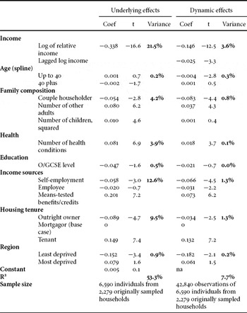
The left panel of Table 4 shows that the underlying relationship linking people's average income over the period and their average deprivation score is rather stronger than could be observed when we had only one wave's set of observations to compare. In general, all the relationships from the cross-sectional model are confirmed, with coefficients of the same sign and a similar order of magnitude. The most striking difference, though, is that the underlying model explains a higher proportion of the variance in the dependent variable: 53 per cent compared with the 37 per cent shown in Table 3. All of the groups of variables are more effective predictors when underlying characteristics are used to analyse underlying outcomes.

TABLE 4.

Underlying and dynamic regressions predicting relative deprivation score (panel models, originally sampled households treated as clusters)

Notes: the column headed ‘variance’ shows the central estimate of the contribution to variance, as discussed in relation to the cross-sectional analysis in the previous table. The dynamic model has fewer observations than the total reported in the text, because the decision to include a lagged income variable reduced the length of the sequences available.

The coefficients from the dynamic (within-effects) model shown in the right-hand side of Table 4 are the longitudinal relationships. A household's deprivation score falls when its income rises, and vice versa. These outcomes are usually interpreted as true causal effects, so it can be concluded that deprivation is at least partly a direct result of a low income. But the income coefficient in the dynamic model is less than half of that observed in the underlying model, indicating that about half of the overall association between income and deprivation is mediated by underlying characteristics of poor households. The model also allows for the possibility that deprivation responds to rises and falls in income a bit sluggishly, perhaps because households tend to smooth their expenditure across periods of rising and falling income (Brewer et al., Reference Brewer, Goodman and Leicester2006). The coefficient on last year's (lagged) income is significant, though not large in relation to the gap between the two models’ estimates for this year's income. Tests of a second and third lagged income variable did not show significant influences.

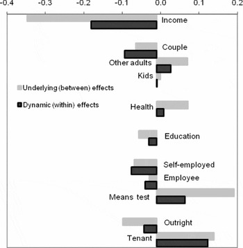
Figure 4 illustrates the differences between the underlying and dynamic coefficients for all the main independent variables. The dynamic effect due to income includes the first lag. Where the dynamic effect (black) is about as strong as the underlying effect (grey), both can be interpreted as causal explanations. So, for example, the analysis suggests that acquiring a partner reduces deprivation and separating increases it. Changing one's employment status, and moving in and out of rented accommodation, are also associated with the expected changes in deprivation scores. On the other hand, the other family composition measures – ill health, education, means-tested benefits and outright ownership – are, like income, only partly associated with transitions into and out of these states, with some underlying characteristics contributing to an explanation of people's current position. Indeed, there is no significant evidence of a longitudinal relationship between number of children and level of deprivation (controlling for income): a highly surprising finding with some potentially controversial policy implications.Footnote ¹²

Figure 4.

Comparison of coefficients from the underlying and dynamic effects models

Notes: 1 The graph is designed to illustrate the differences between the two coefficients for each covariate. It does not illustrate the relative strengths of the predictive power of the different covariates, because they do not use the same units.

2 The within-effects (dynamic) coefficient for income shown here is the sum of the current and the lagged effects from Table 4.

The most striking difference between the two models is, though, their explanatory power, with the overall R² falling from 53 per cent to 8 per cent. And while the crucial income coefficients reduced by about half, their contribution to the variance reduced from 21.5 per cent to 3.6 per cent. This means that while households’ deprivation scores decreased on average when their incomes rose, there was a wide range of variation in their particular experiences: some enjoying a much bigger fall in their deprivation scores, others facing a rise in reported deprivation in spite an improvement in their income. We interpret this range of error in the predicted outcomes in terms of noise in the deprivation variables being analysed: random wobbles either in households’ actual experience, or in the accuracy of their survey responses, which are not substantively important but which interfere with the reliability with which changes in one can be related to changes in the other.

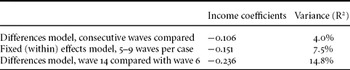
The dynamic model is based on between five and nine pooled observations for each member of the sample, showing how far people's deprivation scores tended to be high during the low-income years of their personal sequence and vice versa. Analysts might be tempted to look for this longitudinal relationship in a transition matrix between two consecutive waves of data. But the first line of Table 5 shows that the relationship between income and deprivation appears even weaker when two consecutive years are compared (though it is still significant). A consecutive differences model – which can be thought of as a dynamic (within-effects) model with only two observations per case – reduces the income coefficient by a third, and the variance explained by getting on for a half. We needed the long run of BHPS data to establish even the weak causal association between income and deprivation reported in Table 4 (dynamic).

TABLE 5.

Three alternative estimates of the longitudinal relationship between income and deprivation

Note: All three models include the complete set of covariates reported in Table 4, except for lagged income.

On the other hand, a differences model comparing two observations eight years apart yielded a substantially larger income coefficient and explanation of variance than the standard dynamic (within-effects) model had estimated.

One explanation for the findings reported in Table 5 is in terms of random measurement error. The true gap in personal experience in neighbouring years will be quite small, and the random error in both dependent and independent variables relatively important, while the true gap between widely spaced years will be larger, with the same absolute random error now relatively unimportant. The evidence based on the widely spaced pairs of years suggests that the dynamic model using all observations may underestimate the true relationships, biased downwards by attenuation. The main methodological lesson is that we may need many observations over a long period to measure the dynamics of deprivation with any accuracy.

Review and conclusions

Although deprivation indicators have been of significant research interest for many years, this is the first study in which the longitudinal dimension has been a main focus. Analysis of deprivation indicators over time sheds much light on the consequences of changing income for families’ welfare.