1 Introduction
We examine the nonlinear resonant excitation of an array of curved oscillating gates in a semi-infinite channel. The gate model is similar to that shown in Mei, Stiassnie & Yue (Reference Mei, Stiassnie and Yue2005), though here we consider a generalised weak horizontal displacement of the gate wetted surface about the vertical plane and the presence of a linear damper exerting a force proportional to the gate velocity. This gives rise to new terms in the evolution equation and to richer dynamics than the case of flat undamped gates.
The array spans the entire channel width, thus the model presented here allows simulation of an infinite periodic array of gates as well (Linton & McIver Reference Linton and McIver2001; Li & Mei Reference Li and Mei2003). This particular configuration admits eigenfrequencies and corresponding homogeneous trapped-mode solutions at the leading order (Mei et al. Reference Mei, Sammarco, Chan and Procaccini1994). Physically, trapped modes of a gate barrier are described by unforced, self-sustained fluid oscillations that decay exponentially from the gates and that do not lose energy through wave radiation (Mei et al. Reference Mei, Stiassnie and Yue2005). We remark that the wave trapping phenomenon is of considerable interest in several applications such as acoustic resonance in pipes (Hein & Koch Reference Hein and Koch2008), gratings (Porter & Evans Reference Porter and Evans1999), thin elastic plates (Porter Reference Porter2007), waveguides (Callan, Linton & Evans Reference Callan, Linton and Evans1991; Linton & Ratcliffe Reference Linton and Ratcliffe2004), open channels (Evans & Linton Reference Evans and Linton1991), cylinders in a channel (Evans & Porter Reference Evans and Porter1997; Utsunomya & Taylor Reference Utsunomya and Taylor1997), edge waves (Blondeaux & Vittori Reference Blondeaux and Vittori1995; Li Reference Li2007), Venice gates (Li & Mei Reference Li and Mei2003; Sammarco, Michele & d’Errico Reference Sammarco, Michele and d’Errico2013), internal waves (Kuznetsov Reference Kuznetsov1993; Nazarov & Videman Reference Nazarov and Videman2009) and wave energy conversion Michele, Sammarco & d’Errico (Reference Michele, Sammarco and d’Errico2018b ).
Linear resonance of trapped modes of a gate barrier in a channel by normally incident waves is not possible because of orthogonality between the modal matrix and the forcing terms (Adamo & Mei Reference Adamo and Mei2005); hence we need to extend the analysis to weakly nonlinear waves by taking into account higher-order effects. Similar considerations apply to edge waves (Guza & Bowen Reference Guza and Bowen1976; Rockliff Reference Rockliff1978), resonance of trapped surface waves around a fixed cylinder (Li & Mei Reference Li and Mei2006), cross-waves (Lichter & Chen Reference Lichter and Chen1987), Faraday waves (Miles Reference Miles1984; Holmes Reference Holmes1986; Gu & Sethna Reference Gu and Sethna1987; Miles & Henderson Reference Miles and Henderson1990) and trapped modes for the Venice gates (Mei et al. Reference Mei, Sammarco, Chan and Procaccini1994; Vittori, Blondeaux & Seminara Reference Vittori, Blondeaux and Seminara1996; Sammarco, Tran & Mei Reference Sammarco, Tran and Mei1997b ; Sammarco et al. Reference Sammarco, Tran, Gottlieb and Mei1997a ).
Here we extend the previous theories by coupling nonlinearity with a small horizontal deviation of the gate surface with respect to the channel depth. We show that this small horizontal deviation of the gate surface produces significant changes in the behaviour of the system. The method of solution adopted here is similar to that used for the Bragg scattering phenomenon of incident waves by bottom ripples (Kirby Reference Kirby1986; Mei, Hara & Naciri Reference Mei, Hara and Naciri1988; Mei et al.
Reference Mei, Stiassnie and Yue2005; Alam, Liu & Yue Reference Alam, Liu and Yue2010). Using perturbation-harmonic expansion up to the third order, we decompose the nonlinear governing equations in a sequence of linear boundary-value problems of order
 $n$
and harmonic
 $m$
(Mei et al.
Reference Mei, Stiassnie and Yue2005; Jordan & Smith Reference Jordan and Smith2011). Gate shape effects give secular terms for the first harmonic at the second order, so that three timing with a slow time scale and a super-slow time scale is necessary (Nayfeh & Mook Reference Nayfeh and Mook1995).
First, we investigate the synchronous resonance mechanism by monochromatic waves with small amplitude and frequency corresponding to the eigenfrequency of the trapped mode. Note that synchronous excitation is not possible for flat gates, because in that case the evolution equation would be damped and unforced. Here, on the contrary, we obtain products between the gate shape function and the second-order terms that force the first harmonic at the third order. We derive the corresponding complex nonlinear evolution equation of the Ginzburg–Landau form (Aranson & Kramer Reference Aranson and Kramer2002; Drazin Reference Drazin2002), which describes the time evolution of the resonated trapped mode. Such an equation is more complicated than that already studied by Sammarco et al. (Reference Sammarco, Tran and Mei1997b ,Reference Sammarco, Tran, Gottlieb and Mei a ) and Michele et al. (Reference Michele, Sammarco and d’Errico2018b ), because it includes new additional terms depending on the shape of the array.
Finally, we apply the theory to the case of an array of surge-type wave energy converters (WECs) with curved geometry. Such bodies oscillate under the action of incident waves and are capable of absorbing energy with potentially large efficiency. For an extensive review we refer to Babarit et al. (Reference Babarit, Hals, Muliawan, Kurniawan, Moan and Krokstad2012), Dias et al. (Reference Dias, Renzi, Gallagher, Sarkar, Wei, Abadie, Cummins and Rafiee2017) and Babarit (Reference Babarit2018). The literature on the hydrodynamic behaviour of gate-type devices is vast and deeply developed by several authors (Linton & McIver Reference Linton and McIver2001; Mei et al. Reference Mei, Stiassnie and Yue2005; Renzi & Dias Reference Renzi and Dias2012, Reference Renzi and Dias2013, Reference Renzi and Dias2014; Sammarco et al. Reference Sammarco, Michele and d’Errico2013; Michele et al. Reference Michele, Sammarco, d’Errico, Renzi, Abdolali, Bellotti and Dias2015; Noad & Porter Reference Noad and Porter2015; Sarkar, Renzi & Dias Reference Sarkar, Renzi and Dias2015; Michele, Sammarco & d’Errico Reference Michele, Sammarco and d’Errico2016a ,Reference Michele, Sammarco and d’Errico b ). Experimental campaigns (Folley, Whittaker & van’t Hoff Reference Folley, Whittaker and van’t Hoff2007; Henry et al. Reference Henry, Doherty, Cameron, Whittaker and Doherty2010; Wilkinson et al. Reference Wilkinson, Whittaker, Thies, Day and Ingram2017) and numerical investigations (Renzi et al. Reference Renzi, Abdolali, Bellotti and Dias2014; Schmitt & Elsaesser Reference Schmitt and Elsaesser2015) are available as well. However, a large part of the theoretical models developed so far on the dynamics of surging WECs neglects nonlinear contributions. This can be unjustified when trapped modes are resonantly excited by incident waves. Indeed, Michele et al. (Reference Michele, Sammarco and d’Errico2018b ) showed that subharmonic resonance and mode competition of trapped natural modes significantly increase energy production of a system of gate-type devices. Furthermore, recent investigations on curved flap-type gates suggest that using curved structure could further improve the economics of WECs by maximising wave power extraction in non-resonant configurations (Hodge et al. Reference Hodge, Bateman, Yuan, Thies and Bruce2017; Michele, Renzi & Sammarco Reference Michele, Renzi and Sammarco2018a ).
We show that nonlinear synchronous resonance of curved WECs yields constructive interactions in terms of generated power that can be significant for design purposes. We remark that this mechanism is not possible for linearised theories or flat WECs. Then we investigate the case of subharmonic resonance and define an optimum criterion to find the power take-off (PTO) coefficient which maximises power extraction. Large efficiency is attained, with the capture factor reaching much greater values than the theoretical maximum of a two-dimensional absorber described by the linear theory (Mei et al. Reference Mei, Stiassnie and Yue2005). However, in this case the performance of curved gates is sub-optimal with respect to that of flat gates.
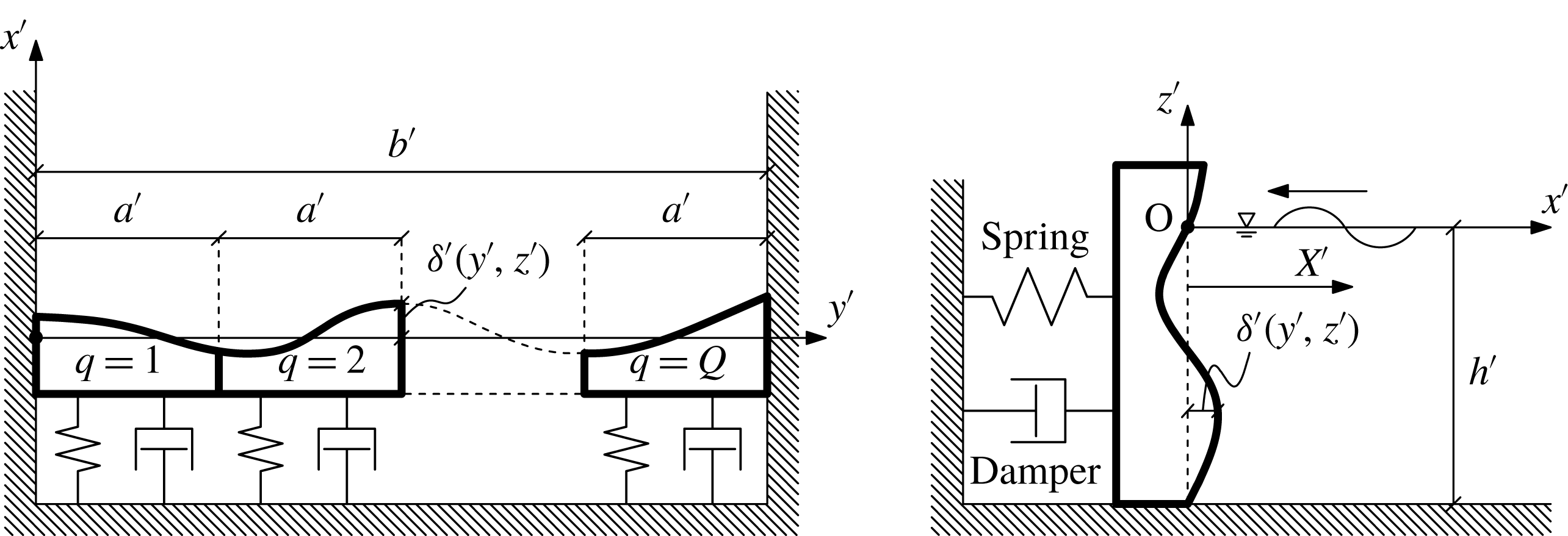
Plan geometry of the system and side view of the gate in physical variables.

2 Governing equations
With reference to figure 1, consider a semi-infinite channel of constant depth
 $h^{\prime }$
and width
 $b^{\prime }$
. Define a Cartesian reference system
 $(x^{\prime },y^{\prime },z^{\prime })$
with the
 $x^{\prime }$
and
 $y^{\prime }$
-axes lying on the undisturbed free surface level and the
 $z^{\prime }$
axis pointing upward. Primes indicate physical variables. At
 $x^{\prime }=0$
rests an array of gates, each with mass
 $M^{\prime }$
and width
 $a^{\prime }$
, allowed to move horizontally (surge) along the channel, under the action of incident harmonic waves. Each gate is connected to the channel back wall by a spring–damper system operating in parallel. The spring has elastic constant
 $C^{\prime }$
, while the linear damper has constant damping
 $\unicode[STIX]{x1D708}^{\prime }$
and exerts a force proportional to the gate velocity. Let us assume incoming waves from
 $x^{\prime }\rightarrow +\infty$
, normally incident to the gates. Let
 $G_{q}$
,
 $q=1,\ldots ,Q$
, denote the
 $q$
th gate and
 $X_{q}^{\prime }$
be the displacement of
 $G_{q}$
positive rightward. Then we can define
 $X^{\prime }(y^{\prime },t^{\prime })=\{X_{1}^{\prime }(t^{\prime }),\ldots ,X_{q}^{\prime }(t^{\prime }),\ldots ,X_{Q}^{\prime }(t^{\prime })\}$
as the displacement function of the entire array. The fluid is assumed to be inviscid and incompressible and the flow irrotational. Hence, the velocity potential
 $\unicode[STIX]{x1D6F7}^{\prime }(x^{\prime },y^{\prime },z^{\prime },t^{\prime })$
satisfies the Laplace equation in the fluid domain
 $\unicode[STIX]{x1D6FA}^{\prime }(x^{\prime },y^{\prime },z^{\prime })$
. The position of the wetted gate surface is described by
 $$\begin{eqnarray}x^{\prime }-X^{\prime }(y^{\prime },t^{\prime })-\unicode[STIX]{x1D6FF}^{\prime }(y^{\prime },z^{\prime })=0,\end{eqnarray}$$
where
 $\unicode[STIX]{x1D6FF}^{\prime }$
denotes the deviation of the array surface from
 $x^{\prime }=0$
. Let
 $A_{T}^{\prime }\ll \unicode[STIX]{x1D706}^{\prime }$
be the scale of the free-surface trapped oscillations,
 $\unicode[STIX]{x1D706}^{\prime }$
the wavelength,
 $\unicode[STIX]{x1D714}^{\prime }$
the eigenfrequency of the natural mode and
 $g^{\prime }$
the acceleration due to gravity. Then introduce the following non-dimensional quantities:
 $$\begin{eqnarray}\left.\begin{array}{@{}c@{}}(x,y,z)=(x^{\prime },y^{\prime },z^{\prime })/\unicode[STIX]{x1D706}^{\prime },\quad \unicode[STIX]{x1D6F7}=\unicode[STIX]{x1D6F7}^{\prime }/(A_{T}^{\prime }\unicode[STIX]{x1D714}^{\prime }\unicode[STIX]{x1D706}^{\prime }),\quad \unicode[STIX]{x1D701}=\unicode[STIX]{x1D701}^{\prime }/A_{T}^{\prime },\quad t=t^{\prime }\unicode[STIX]{x1D714}^{\prime },\\ (a,b,h)=(a^{\prime },b^{\prime },h^{\prime })/\unicode[STIX]{x1D706}^{\prime },\quad X=X^{\prime }/A_{T}^{\prime },\quad \unicode[STIX]{x1D6FF}=\unicode[STIX]{x1D6FF}^{\prime }/\unicode[STIX]{x1D6FF}_{g}^{\prime },\quad G=g^{\prime }/(\unicode[STIX]{x1D714}^{\prime 2}\unicode[STIX]{x1D706}^{\prime }),\end{array}\right\}\end{eqnarray}$$
where
 $\unicode[STIX]{x1D701}^{\prime }$
is the free-surface elevation,
 $\unicode[STIX]{x1D6FF}_{g}^{\prime }=\mathit{O}(A_{T}^{\prime })$
the length scale for
 $\unicode[STIX]{x1D6FF}^{\prime }$
and
 $G$
the non-dimensional eigenfrequency. Let the following length ratios be much smaller than unity
 $$\begin{eqnarray}\unicode[STIX]{x1D716}=A_{T}^{\prime }/\unicode[STIX]{x1D706}^{\prime }\ll 1,\quad \unicode[STIX]{x1D707}=\unicode[STIX]{x1D6FF}_{g}^{\prime }/\unicode[STIX]{x1D706}^{\prime }\ll 1,\quad \unicode[STIX]{x1D707}=\mathit{O}(\unicode[STIX]{x1D716}).\end{eqnarray}$$
Since the derivatives of
 $\unicode[STIX]{x1D6FF}^{\prime }$
with respect to the coordinates
 $(y^{\prime },z^{\prime })$
are of order
 $\unicode[STIX]{x1D716}$
as well, the latter assumptions imply that the shape of the array must be smooth and regular.
Using the dimensionless variables (2.2)–(2.3), we derive the following governing equations, boundary conditions and equation of motion in non-dimensional form. The Laplace and Bernoulli equations in the fluid domain are, respectively,
 $$\begin{eqnarray}\displaystyle & \unicode[STIX]{x1D6FB}^{2}\unicode[STIX]{x1D6F7}=0, & \displaystyle\end{eqnarray}$$
 $$\begin{eqnarray}\displaystyle & \displaystyle -\frac{p^{\prime }}{\unicode[STIX]{x1D70C}^{\prime }\unicode[STIX]{x1D714}^{\prime 2}\unicode[STIX]{x1D706}^{\prime 2}}=Gz+\unicode[STIX]{x1D716}\unicode[STIX]{x1D6F7}_{t}+\unicode[STIX]{x1D716}^{2}\frac{1}{2}|\unicode[STIX]{x1D735}\unicode[STIX]{x1D6F7}|^{2}, & \displaystyle\end{eqnarray}$$
where
 $\unicode[STIX]{x1D70C}^{\prime }$
is the fluid density, while subscripts denote differentiation with respect to the relevant variable. The dynamic and mixed boundary conditions on the free surface read, respectively,
 $$\begin{eqnarray}-G\unicode[STIX]{x1D701}=\unicode[STIX]{x1D6F7}_{t}+\unicode[STIX]{x1D716}{\textstyle \frac{1}{2}}|\unicode[STIX]{x1D735}\unicode[STIX]{x1D6F7}|^{2},\quad z=\unicode[STIX]{x1D716}\unicode[STIX]{x1D701},\end{eqnarray}$$
 $$\begin{eqnarray}\unicode[STIX]{x1D6F7}_{tt}+G\unicode[STIX]{x1D6F7}_{z}+\unicode[STIX]{x1D716}|\unicode[STIX]{x1D735}\unicode[STIX]{x1D6F7}|_{t}^{2}+\unicode[STIX]{x1D716}^{2}{\textstyle \frac{1}{2}}\unicode[STIX]{x1D735}\unicode[STIX]{x1D6F7}\boldsymbol{\cdot }\unicode[STIX]{x1D735}|\unicode[STIX]{x1D735}\unicode[STIX]{x1D6F7}|^{2}=0,\quad z=\unicode[STIX]{x1D716}\unicode[STIX]{x1D701},\end{eqnarray}$$
while the no-flux conditions at the bottom and channel walls require
 $$\begin{eqnarray}\displaystyle & \unicode[STIX]{x1D6F7}_{z}=0,\quad z=-h, & \displaystyle\end{eqnarray}$$
 $$\begin{eqnarray}\displaystyle & \unicode[STIX]{x1D6F7}_{y}=0,\quad y=0\quad \text{and}\quad y=b. & \displaystyle\end{eqnarray}$$
The kinematic condition on the array surface
 $$\begin{eqnarray}x=\unicode[STIX]{x1D716}X+\unicode[STIX]{x1D707}\unicode[STIX]{x1D6FF},\end{eqnarray}$$
can be now written as
 $$\begin{eqnarray}\unicode[STIX]{x1D6F7}_{x}=X_{t}+\unicode[STIX]{x1D707}(\unicode[STIX]{x1D6F7}_{y}\unicode[STIX]{x1D6FF}_{y}+\unicode[STIX]{x1D6F7}_{z}\unicode[STIX]{x1D6FF}_{z}).\end{eqnarray}$$
The equation of motion of the
 $q$
th curved gate coupled with a linear damper is given by
 $$\begin{eqnarray}\unicode[STIX]{x1D716}MX_{q,tt}+\unicode[STIX]{x1D716}CGX_{q}+\unicode[STIX]{x1D716}^{3}\unicode[STIX]{x1D708}X_{q,t}=\int _{(q-1)a}^{qa}\,\text{d}y\left\{\int _{-1}^{\unicode[STIX]{x1D716}\unicode[STIX]{x1D701}}\,\text{d}z\left(\unicode[STIX]{x1D716}\unicode[STIX]{x1D6F7}_{t}+\unicode[STIX]{x1D716}^{2}\frac{1}{2}|\unicode[STIX]{x1D735}\unicode[STIX]{x1D6F7}|^{2}\right)+\int _{0}^{\unicode[STIX]{x1D716}\unicode[STIX]{x1D701}}Gz\,\text{d}z\right\},\end{eqnarray}$$
where
 $M=M^{\prime }/(\unicode[STIX]{x1D70C}^{\prime }\unicode[STIX]{x1D706}^{\prime 3})$
is the non-dimensional mass of the gate,
 $C=C^{\prime }/(g^{\prime }\unicode[STIX]{x1D70C}^{\prime }\unicode[STIX]{x1D706}^{\prime 2})$
the non-dimensional stiffness of the spring and
 $\unicode[STIX]{x1D708}=\unicode[STIX]{x1D708}^{\prime }/(A_{T}^{\prime 2}\unicode[STIX]{x1D714}^{\prime }\unicode[STIX]{x1D70C}^{\prime }\unicode[STIX]{x1D706}^{\prime })$
the non-dimensional damping coefficient. In (2.12) we have assumed the contribution due to the damping force on the gate motion to be small if compared to the other terms. Large values of
 $\unicode[STIX]{x1D708}^{\prime }$
comparable with leading-order terms would render the equation of motion at
 $\mathit{O}(1)$
damped and unforced, so that a trapped-mode solution would not be possible anymore (Michele et al.
Reference Michele, Sammarco and d’Errico2018b
). Assuming
 $A_{T}^{\prime }\sim \mathit{O}(1)~\text{m}$
,
 $\unicode[STIX]{x1D714}^{\prime }\sim \mathit{O}(1)~\text{rad}~\text{s}^{-1}$
,
 $\unicode[STIX]{x1D706}^{\prime }\sim \mathit{O}(10){-}\mathit{O}(10^{2})~\text{m}$
, the values of
 $\unicode[STIX]{x1D708}^{\prime }$
that satisfy the scale above should be of order
 $\mathit{O}(10^{4}){-}\mathit{O}(10^{5})~\text{kg}~\text{s}^{-1}$
. In § 5 we demonstrate that these orders of magnitude are physically congruent with power take-off systems for practical engineering applications (Mei et al.
Reference Mei, Stiassnie and Yue2005).
The free-surface boundary conditions are evaluated in correspondence of
 $z=\unicode[STIX]{x1D716}\unicode[STIX]{x1D701}$
, thus Taylor expanding (2.6) and (2.7) about
 $z=0$
up to
 $\mathit{O}(\unicode[STIX]{x1D716}^{2})$
yields, respectively,
 $$\begin{eqnarray}-G\unicode[STIX]{x1D701}=[\unicode[STIX]{x1D6F7}_{t}]_{z=0}+\unicode[STIX]{x1D716}\unicode[STIX]{x1D701}[\unicode[STIX]{x1D6F7}_{tz}]_{z=0}+\unicode[STIX]{x1D716}^{2}\frac{\unicode[STIX]{x1D701}^{2}}{2}[\unicode[STIX]{x1D6F7}_{tzz}]_{z=0}+\unicode[STIX]{x1D716}\frac{1}{2}[|\unicode[STIX]{x1D735}\unicode[STIX]{x1D6F7}|^{2}]_{z=0}+\unicode[STIX]{x1D716}^{2}\frac{\unicode[STIX]{x1D701}}{2}[|\unicode[STIX]{x1D735}\unicode[STIX]{x1D6F7}|_{z}^{2}]_{z=0},\end{eqnarray}$$
 $$\begin{eqnarray}\displaystyle & & \displaystyle [\unicode[STIX]{x1D6F7}_{tt}+G\unicode[STIX]{x1D6F7}_{z}]_{z=0}+\unicode[STIX]{x1D716}\unicode[STIX]{x1D701}[\unicode[STIX]{x1D6F7}_{ttz}+G\unicode[STIX]{x1D6F7}_{zz}]_{z=0}+\unicode[STIX]{x1D716}^{2}\frac{\unicode[STIX]{x1D701}^{2}}{2}[\unicode[STIX]{x1D6F7}_{ttzz}+G\unicode[STIX]{x1D6F7}_{zzz}]_{z=0}+\unicode[STIX]{x1D716}[|\unicode[STIX]{x1D735}\unicode[STIX]{x1D6F7}|_{t}^{2}]_{z=0}\nonumber\\ \displaystyle & & \displaystyle \quad +\,\unicode[STIX]{x1D716}^{2}\unicode[STIX]{x1D701}[|\unicode[STIX]{x1D735}\unicode[STIX]{x1D6F7}|_{tz}^{2}]_{z=0}+\unicode[STIX]{x1D716}^{2}\frac{1}{2}[\unicode[STIX]{x1D735}\unicode[STIX]{x1D6F7}\boldsymbol{\cdot }\unicode[STIX]{x1D735}|\unicode[STIX]{x1D735}\unicode[STIX]{x1D6F7}|^{2}]_{z=0}=0.\end{eqnarray}$$
Similarly, the kinematic boundary condition on the gate surface can be Taylor expanded about
 $x=0$
:
 $$\begin{eqnarray}\displaystyle [\unicode[STIX]{x1D6F7}_{x}]_{x=0} & = & \displaystyle X_{t}-(\unicode[STIX]{x1D716}X+\unicode[STIX]{x1D707}\unicode[STIX]{x1D6FF})[\unicode[STIX]{x1D6F7}_{xx}]_{x=0}-\frac{1}{2}(\unicode[STIX]{x1D716}X+\unicode[STIX]{x1D707}\unicode[STIX]{x1D6FF})^{2}[\unicode[STIX]{x1D6F7}_{xxx}]_{x=0}\nonumber\\ \displaystyle & & \displaystyle +\,\unicode[STIX]{x1D707}[\unicode[STIX]{x1D6F7}_{y}\unicode[STIX]{x1D6FF}_{y}+\unicode[STIX]{x1D6F7}_{z}\unicode[STIX]{x1D6FF}_{z}]_{x=0}+\unicode[STIX]{x1D707}(\unicode[STIX]{x1D716}X+\unicode[STIX]{x1D707}\unicode[STIX]{x1D6FF})[\unicode[STIX]{x1D6F7}_{xy}\unicode[STIX]{x1D6FF}_{y}+\unicode[STIX]{x1D6F7}_{xz}\unicode[STIX]{x1D6FF}_{z}]_{x=0}.\end{eqnarray}$$
Finally the equation of motion (2.12) becomes:
 $$\begin{eqnarray}\displaystyle & & \displaystyle MX_{q,tt}+GCX_{q}+\unicode[STIX]{x1D716}^{2}\unicode[STIX]{x1D708}X_{q,t}=\int _{(q-1)a}^{qa}\,\text{d}y\int _{-1}^{0}\,\text{d}z\left\{\unicode[STIX]{x1D6F7}_{t}+\unicode[STIX]{x1D716}\left[\unicode[STIX]{x1D6F7}_{tx}\left(X+\frac{\unicode[STIX]{x1D707}\unicode[STIX]{x1D6FF}}{\unicode[STIX]{x1D716}}\right)+\frac{|\unicode[STIX]{x1D735}\unicode[STIX]{x1D6F7}|^{2}}{2}\right]\right.\nonumber\\ \displaystyle & & \displaystyle \quad +\left.\unicode[STIX]{x1D716}^{2}\left(X+\frac{\unicode[STIX]{x1D707}\unicode[STIX]{x1D6FF}}{\unicode[STIX]{x1D716}}\right)\left[\frac{\unicode[STIX]{x1D6F7}_{txx}}{2}\left(X+\frac{\unicode[STIX]{x1D707}\unicode[STIX]{x1D6FF}}{\unicode[STIX]{x1D716}}\right)+\frac{|\unicode[STIX]{x1D735}\unicode[STIX]{x1D6F7}|_{x}^{2}}{2}\right]\right\}_{x=0}+\unicode[STIX]{x1D716}\int _{(q-1)a}^{qa}\,\text{d}y\left\{\left[\frac{G\unicode[STIX]{x1D701}^{2}}{2}+\unicode[STIX]{x1D6F7}_{t}\unicode[STIX]{x1D701}\right]\right.\nonumber\\ \displaystyle & & \displaystyle \quad +\left.\unicode[STIX]{x1D716}\left[\left(G\unicode[STIX]{x1D701}\unicode[STIX]{x1D701}_{x}+\unicode[STIX]{x1D6F7}_{tx}\unicode[STIX]{x1D701}\right)\left(X+\frac{\unicode[STIX]{x1D707}\unicode[STIX]{x1D6FF}}{\unicode[STIX]{x1D716}}\right)+\frac{\unicode[STIX]{x1D6F7}_{tz}\unicode[STIX]{x1D701}^{2}}{2}+\frac{\unicode[STIX]{x1D701}|\unicode[STIX]{x1D735}\unicode[STIX]{x1D6F7}|^{2}}{2}\right]\right\}_{x=0,z=0}.\end{eqnarray}$$
3 Multiple-scale analysis and three timing
Let us introduce the following expansions of the non-dimensional velocity potential, free-surface elevation and gate oscillation:
 $$\begin{eqnarray}\displaystyle & \unicode[STIX]{x1D6F7}=\unicode[STIX]{x1D6F7}_{1}(x,y,z,t,t_{1},t_{2})+\unicode[STIX]{x1D716}\unicode[STIX]{x1D6F7}_{2}(x,y,z,t,t_{1},t_{2})+\unicode[STIX]{x1D716}^{2}\unicode[STIX]{x1D6F7}_{3}(x,y,z,t,t_{1},t_{2})+\mathit{O}(\unicode[STIX]{x1D716}^{3}),\qquad & \displaystyle\end{eqnarray}$$
 $$\begin{eqnarray}\displaystyle & \unicode[STIX]{x1D701}=\unicode[STIX]{x1D701}_{1}(x,y,t,t_{1},t_{2})+\unicode[STIX]{x1D716}\unicode[STIX]{x1D701}_{2}(x,y,t,t_{1},t_{2})+\unicode[STIX]{x1D716}^{2}\unicode[STIX]{x1D701}_{3}(x,y,t,t_{1},t_{2})+\mathit{O}(\unicode[STIX]{x1D716}^{3}), & \displaystyle\end{eqnarray}$$
 $$\begin{eqnarray}\displaystyle & X_{q}=X_{q,1}(t,t_{1},t_{2})+\unicode[STIX]{x1D716}X_{q,2}(t,t_{1},t_{2})+\unicode[STIX]{x1D716}^{2}X_{q,3}(t,t_{1},t_{2})+\mathit{O}(\unicode[STIX]{x1D716}^{3}), & \displaystyle\end{eqnarray}$$
 $$\begin{eqnarray}\displaystyle & X=X_{1}(y,t,t_{1},t_{2})+\unicode[STIX]{x1D716}X_{2}(y,t,t_{1},t_{2})+\unicode[STIX]{x1D716}^{2}X_{3}(y,t,t_{1},t_{2})+\mathit{O}(\unicode[STIX]{x1D716}^{3}), & \displaystyle\end{eqnarray}$$
where
 $t_{1}=\unicode[STIX]{x1D716}t$
and
 $t_{2}=\unicode[STIX]{x1D716}^{2}t$
denote two slow time scales of the modal amplitude growth. Unlike the case of Michele et al. (Reference Michele, Sammarco and d’Errico2018b
), the three-timing assumption is necessary here because of the presence in the governing equations of terms representing the shape of the array. These terms correspond to a resonant forcing for the first-harmonic solution at the second order, so that a solvability condition at
 $\mathit{O}(\unicode[STIX]{x1D716})$
must be applied in order to avoid secularity. The three time scales add terms in the evolution equation for the modal amplitude at the third order
 $\mathit{O}(\unicode[STIX]{x1D716}^{2})$
and the corresponding stability analysis for the equilibrium states increases in complexity. Usage of the expansions (3.1)–(3.4) for the unknowns yields for
 $n=1,2,3,$
the following equations.
Laplace’s equation:
 $$\begin{eqnarray}\unicode[STIX]{x1D6FB}^{2}\unicode[STIX]{x1D6F7}_{n}=0,\quad \text{in }\unicode[STIX]{x1D6FA}.\end{eqnarray}$$
Free-surface dynamic condition:
 $$\begin{eqnarray}-G\unicode[STIX]{x1D701}_{n}=\unicode[STIX]{x1D6F7}_{n_{t}}+{\mathcal{B}}_{n},\quad z=0,\end{eqnarray}$$
where
 $$\begin{eqnarray}{\mathcal{B}}_{1}=0,\quad {\mathcal{B}}_{2}=\unicode[STIX]{x1D6F7}_{1_{t_{1}}}+\unicode[STIX]{x1D6F7}_{1_{tz}}\unicode[STIX]{x1D701}_{1}+{\textstyle \frac{1}{2}}|\unicode[STIX]{x1D735}\unicode[STIX]{x1D6F7}_{1}|^{2},\end{eqnarray}$$
 $$\begin{eqnarray}{\mathcal{B}}_{3}=\unicode[STIX]{x1D6F7}_{1_{t2}}+\unicode[STIX]{x1D6F7}_{2_{t_{1}}}+\unicode[STIX]{x1D6F7}_{1_{t_{1}z}}\unicode[STIX]{x1D701}_{1}+\unicode[STIX]{x1D6F7}_{1_{tz}}\unicode[STIX]{x1D701}_{2}+\unicode[STIX]{x1D6F7}_{2_{tz}}\unicode[STIX]{x1D701}_{1}+\frac{\unicode[STIX]{x1D6F7}_{1_{tzz}}\unicode[STIX]{x1D701}_{1}^{2}}{2}+\unicode[STIX]{x1D735}\unicode[STIX]{x1D6F7}_{1}\boldsymbol{\cdot }\unicode[STIX]{x1D735}\unicode[STIX]{x1D6F7}_{2}+\frac{\unicode[STIX]{x1D701}_{1}}{2}|\unicode[STIX]{x1D735}\unicode[STIX]{x1D6F7}_{1}|_{z}^{2}.\quad\end{eqnarray}$$
Free-surface mixed condition:
 $$\begin{eqnarray}\unicode[STIX]{x1D6F7}_{n_{tt}}+G\unicode[STIX]{x1D6F7}_{n_{z}}={\mathcal{F}}_{n},\quad z=0,\end{eqnarray}$$
where
 $$\begin{eqnarray}{\mathcal{F}}_{1}=0,\quad {\mathcal{F}}_{2}=-2\unicode[STIX]{x1D6F7}_{1_{tt_{1}}}-\unicode[STIX]{x1D701}_{1}(\unicode[STIX]{x1D6F7}_{1_{ttz}}+G\unicode[STIX]{x1D6F7}_{1_{zz}})-|\unicode[STIX]{x1D735}\unicode[STIX]{x1D6F7}_{1}|_{t}^{2},\end{eqnarray}$$
 $$\begin{eqnarray}\displaystyle {\mathcal{F}}_{3} & = & \displaystyle -2\unicode[STIX]{x1D6F7}_{1_{tt_{2}}}-2\unicode[STIX]{x1D6F7}_{2_{tt_{1}}}-\unicode[STIX]{x1D6F7}_{1_{t_{1}t_{1}}}-2\unicode[STIX]{x1D6F7}_{1_{tzt_{1}}}\unicode[STIX]{x1D701}_{1}-\unicode[STIX]{x1D701}_{2}(\unicode[STIX]{x1D6F7}_{1_{ttz}}+G\unicode[STIX]{x1D6F7}_{1_{zz}})-\unicode[STIX]{x1D701}_{1}(\unicode[STIX]{x1D6F7}_{2_{ttz}}+G\unicode[STIX]{x1D6F7}_{2_{zz}})\nonumber\\ \displaystyle & & \displaystyle -\,\frac{\unicode[STIX]{x1D701}_{1}^{2}}{2}(\unicode[STIX]{x1D6F7}_{1_{ttzz}}+G\unicode[STIX]{x1D6F7}_{1_{zzz}})-2(\unicode[STIX]{x1D735}\unicode[STIX]{x1D6F7}_{1}\boldsymbol{\cdot }\unicode[STIX]{x1D735}\unicode[STIX]{x1D6F7}_{2})_{t}-\unicode[STIX]{x1D701}_{1}|\unicode[STIX]{x1D735}\unicode[STIX]{x1D6F7}_{1}|_{tz}^{2}-\frac{1}{2}\unicode[STIX]{x1D735}\unicode[STIX]{x1D6F7}_{1}\boldsymbol{\cdot }\unicode[STIX]{x1D735}|\unicode[STIX]{x1D735}\unicode[STIX]{x1D6F7}_{1}|^{2}\nonumber\\ \displaystyle & & \displaystyle -\,|\unicode[STIX]{x1D735}\unicode[STIX]{x1D6F7}_{1}|_{t_{1}}^{2}.\end{eqnarray}$$
No-flux boundary condition at the horizontal bottom:
 $$\begin{eqnarray}\unicode[STIX]{x1D6F7}_{n_{z}}=0,\quad z=-h.\end{eqnarray}$$
No-flux boundary condition on the channel vertical walls:
 $$\begin{eqnarray}\unicode[STIX]{x1D6F7}_{n_{y}}=0,\quad y=0\quad \text{and}\quad y=b.\end{eqnarray}$$
Kinematic condition on the array surface:
 $$\begin{eqnarray}\unicode[STIX]{x1D6F7}_{n_{x}}=X_{n_{t}}+{\mathcal{G}}_{n},\quad x=0,\end{eqnarray}$$
where
 $$\begin{eqnarray}{\mathcal{G}}_{1}=0,\quad {\mathcal{G}}_{2}=X_{1_{t_{1}}}-\unicode[STIX]{x1D6F7}_{1_{xx}}\left(X_{1}+\frac{\unicode[STIX]{x1D707}\unicode[STIX]{x1D6FF}}{\unicode[STIX]{x1D716}}\right)+\frac{\unicode[STIX]{x1D707}}{\unicode[STIX]{x1D716}}(\unicode[STIX]{x1D6F7}_{1_{y}}\unicode[STIX]{x1D6FF}_{y}+\unicode[STIX]{x1D6F7}_{1_{z}}\unicode[STIX]{x1D6FF}_{z}),\end{eqnarray}$$
 $$\begin{eqnarray}\displaystyle {\mathcal{G}}_{3} & = & \displaystyle X_{1_{t_{2}}}+X_{2_{t_{1}}}-\unicode[STIX]{x1D6F7}_{1_{xx}}X_{2}-\unicode[STIX]{x1D6F7}_{2_{xx}}\left(X_{1}+\frac{\unicode[STIX]{x1D707}\unicode[STIX]{x1D6FF}}{\unicode[STIX]{x1D716}}\right)-\frac{\unicode[STIX]{x1D6F7}_{1_{xxx}}}{2}\left(X_{1}+\frac{\unicode[STIX]{x1D707}\unicode[STIX]{x1D6FF}}{\unicode[STIX]{x1D716}}\right)^{2}\nonumber\\ \displaystyle & & \displaystyle +\,\frac{\unicode[STIX]{x1D707}}{\unicode[STIX]{x1D716}}(\unicode[STIX]{x1D6F7}_{2_{y}}\unicode[STIX]{x1D6FF}_{y}+\unicode[STIX]{x1D6F7}_{2_{z}}\unicode[STIX]{x1D6FF}_{z})+\frac{\unicode[STIX]{x1D707}}{\unicode[STIX]{x1D716}}(\unicode[STIX]{x1D6F7}_{1_{xy}}\unicode[STIX]{x1D6FF}_{y}+\unicode[STIX]{x1D6F7}_{1_{xz}}\unicode[STIX]{x1D6FF}_{z})\left(X_{1}+\frac{\unicode[STIX]{x1D707}\unicode[STIX]{x1D6FF}}{\unicode[STIX]{x1D716}}\right).\end{eqnarray}$$
Equation of motion of the
 $q$
th gate:
 $$\begin{eqnarray}MX_{q,n_{tt}}+GCX_{q,n}=\int _{(q-1)a}^{qa}\,\text{d}y\int _{-1}^{0}\unicode[STIX]{x1D6F7}_{n_{t}}\,\text{d}z+{\mathcal{D}}_{n},\end{eqnarray}$$
where
 $$\begin{eqnarray}\displaystyle {\mathcal{D}}_{1}=0, & & \displaystyle\end{eqnarray}$$
 $$\begin{eqnarray}\displaystyle {\mathcal{D}}_{2} & = & \displaystyle -2MX_{1_{tt_{1}}}+\int _{(q-1)a}^{qa}\,\text{d}y\left\{G\frac{\unicode[STIX]{x1D701}_{1}^{2}}{2}+\unicode[STIX]{x1D6F7}_{1_{t}}\unicode[STIX]{x1D701}_{1}\right\}_{x=0,z=0}\nonumber\\ \displaystyle & & \displaystyle +\,\int _{(q-1)a}^{qa}\,\text{d}y\int _{-1}^{0}\,\text{d}z\left\{\unicode[STIX]{x1D6F7}_{1_{t_{1}}}+\unicode[STIX]{x1D6F7}_{1_{tx}}\left(X_{1}+\frac{\unicode[STIX]{x1D707}\unicode[STIX]{x1D6FF}}{\unicode[STIX]{x1D716}}\right)+\frac{1}{2}|\unicode[STIX]{x1D735}\unicode[STIX]{x1D6F7}_{1}|^{2}\right\}_{x=0},\end{eqnarray}$$
 $$\begin{eqnarray}\displaystyle {\mathcal{D}}_{3} & = & \displaystyle -M(2X_{1_{tt_{2}}}+2X_{2_{tt_{1}}}+X_{1_{t_{1}t_{1}}})+\int _{(q-1)a}^{qa}\,\text{d}y\left\{G\unicode[STIX]{x1D701}_{1}\unicode[STIX]{x1D701}_{2}+\frac{\unicode[STIX]{x1D6F7}_{1_{tz}}\unicode[STIX]{x1D701}_{1}^{2}}{2}+\unicode[STIX]{x1D6F7}_{1_{t}}\unicode[STIX]{x1D701}_{2}+\unicode[STIX]{x1D6F7}_{2_{t}}\unicode[STIX]{x1D701}_{1}\right.\nonumber\\ \displaystyle & & \displaystyle +\left.\unicode[STIX]{x1D6F7}_{1_{t_{1}}}\unicode[STIX]{x1D701}_{1}+\unicode[STIX]{x1D6F7}_{1_{tx}}\unicode[STIX]{x1D701}_{1}\left(X_{1}+\frac{\unicode[STIX]{x1D707}\unicode[STIX]{x1D6FF}}{\unicode[STIX]{x1D716}}\right)+\frac{\unicode[STIX]{x1D701}_{1}}{2}|\unicode[STIX]{x1D735}\unicode[STIX]{x1D6F7}_{1}|^{2}+G\unicode[STIX]{x1D701}_{1}\unicode[STIX]{x1D701}_{1_{x}}\left(X_{1}+\frac{\unicode[STIX]{x1D707}\unicode[STIX]{x1D6FF}}{\unicode[STIX]{x1D716}}\right)\right\}_{x=0,z=0}\nonumber\\ \displaystyle & & \displaystyle +\,\int _{(q-1)a}^{qa}\,\text{d}y\int _{-1}^{0}\,\text{d}z\left\{\unicode[STIX]{x1D6F7}_{1_{t_{2}}}+\unicode[STIX]{x1D6F7}_{2_{t_{1}}}+\unicode[STIX]{x1D6F7}_{1_{tx}}X_{2}+\unicode[STIX]{x1D735}\unicode[STIX]{x1D6F7}_{1}\boldsymbol{\cdot }\unicode[STIX]{x1D735}\unicode[STIX]{x1D6F7}_{2}+\frac{\unicode[STIX]{x1D6F7}_{1_{txx}}}{2}\left(X_{1}+\frac{\unicode[STIX]{x1D707}\unicode[STIX]{x1D6FF}}{\unicode[STIX]{x1D716}}\right)^{2}\right.\nonumber\\ \displaystyle & & \displaystyle +\left.\left(\unicode[STIX]{x1D6F7}_{2_{tx}}+\unicode[STIX]{x1D6F7}_{1_{t_{1}x}}+\frac{1}{2}|\unicode[STIX]{x1D735}\unicode[STIX]{x1D6F7}_{1}|_{x}^{2}\right)\left(X_{1}+\frac{\unicode[STIX]{x1D707}\unicode[STIX]{x1D6FF}}{\unicode[STIX]{x1D716}}\right)\vphantom{\left(X_{1}+\frac{\unicode[STIX]{x1D707}\unicode[STIX]{x1D6FF}}{\unicode[STIX]{x1D716}}\right)^{2}}\right\}_{x=0}-\unicode[STIX]{x1D708}X_{q,1_{t}}.\end{eqnarray}$$
Because of harmonic motion, higher-order solutions imply higher harmonics (Jordan & Smith Reference Jordan and Smith2011). Hence we return to physical variables except for
 $t_{1}$
and
 $t_{2}$
, omit the primes for convenience and assume the following harmonic expansions of the unknowns:
 $$\begin{eqnarray}\{\unicode[STIX]{x1D6F7}_{n},\unicode[STIX]{x1D701}_{n},X_{q,n},X_{n}\}=\mathop{\sum }_{m=0}^{n}\{\unicode[STIX]{x1D719}_{nm},\unicode[STIX]{x1D702}_{nm},\unicode[STIX]{x1D712}_{q,nm},\unicode[STIX]{x1D712}_{nm}\}\text{e}^{-\text{i}m\unicode[STIX]{x1D714}t}+\ast ,\end{eqnarray}$$
where the symbol
 $\ast$
indicates the complex conjugate of the terms inside the series. Substitution of the latter expansion into the governing equation and boundary conditions allows us to split the nonlinear problem in a sequence of linear boundary-value problems of order
 $n$
and harmonic
 $m$
:
 $$\begin{eqnarray}\displaystyle & \unicode[STIX]{x1D6FB}^{2}\unicode[STIX]{x1D719}_{nm}=0,\quad \text{in }\unicode[STIX]{x1D6FA}, & \displaystyle\end{eqnarray}$$
 $$\begin{eqnarray}\displaystyle & \unicode[STIX]{x1D719}_{nm_{z}}=\unicode[STIX]{x1D719}_{nm}{\displaystyle \frac{m^{2}\unicode[STIX]{x1D714}^{2}}{g}}+{\mathcal{F}}_{nm},\quad z=0, & \displaystyle\end{eqnarray}$$
 $$\begin{eqnarray}\displaystyle & \unicode[STIX]{x1D702}_{nm}=\unicode[STIX]{x1D719}_{nm}{\displaystyle \frac{\text{i}m\unicode[STIX]{x1D714}}{g}}+{\mathcal{B}}_{nm},\quad z=0, & \displaystyle\end{eqnarray}$$
 $$\begin{eqnarray}\displaystyle & \unicode[STIX]{x1D719}_{nm_{z}}=0,\quad z=-h, & \displaystyle\end{eqnarray}$$
 $$\begin{eqnarray}\displaystyle & \unicode[STIX]{x1D719}_{nm_{y}}=0,\quad y=0,y=b, & \displaystyle\end{eqnarray}$$
 $$\begin{eqnarray}\displaystyle & \unicode[STIX]{x1D719}_{nm_{x}}=-\text{i}m\unicode[STIX]{x1D714}\unicode[STIX]{x1D712}_{nm}+{\mathcal{G}}_{nm},\quad x=0. & \displaystyle\end{eqnarray}$$
The latter must be solved jointly with the equation of motion for each gate
 $G_{q}$
(3.17), which now becomes:
 $$\begin{eqnarray}-m^{2}\unicode[STIX]{x1D714}^{2}M\unicode[STIX]{x1D712}_{q,nm}+C\unicode[STIX]{x1D712}_{q,nm}=-\text{i}m\unicode[STIX]{x1D714}\unicode[STIX]{x1D70C}\int _{(q-1)a}^{qa}\,\text{d}y\int _{-h}^{0}\unicode[STIX]{x1D719}_{nm}\,\text{d}z+{\mathcal{D}}_{nm},\end{eqnarray}$$
where the forcing terms
 ${\mathcal{F}}_{nm}$
,
 ${\mathcal{B}}_{nm}$
,
 ${\mathcal{G}}_{nm}$
and the
 ${\mathcal{D}}_{nm}$
values are defined for each order
 $n$
and harmonic
 $m$
in appendix A. Having obtained the governing equations at the different orders, we are now in a position to investigate the nonlinear synchronous excitation of trapped modes.
4 Nonlinear synchronous excitation of a single trapped mode
In this section we analyse the synchronous excitation of a single trapped mode by small incident waves at the second order
 $\mathit{O}(\unicode[STIX]{x1D716})$
. We remark that such nonlinear dynamics is peculiar to curved gates and nonlinear resonance mechanisms. Indeed, trapped modes cannot be resonated in linear theories by normally incident waves because of orthogonality between the modal matrix and forcing terms, while flat-gate systems do not allow nonlinear synchronous excitation when the incident waves are small compared to the trapped wave field. This is due to the absence of first-harmonic terms at the third order that include the forcing incident wave potential. In that case, the evolution equation would be damped and unforced and the corresponding solution would be given by the trivial stable state.
As in Michele et al. (Reference Michele, Sammarco and d’Errico2018b
), we perform an asymptotic analysis up to the third order
 $\mathit{O}(\unicode[STIX]{x1D716}^{2})$
. For the sake of brevity, we show the solutions of each boundary-value problem of order
 $n$
and harmonic
 $m$
in appendix A. We obtain that the second-order inhomogeneous problem is forced by products between the first-order solution
 $\unicode[STIX]{x1D719}_{11}$
and the gate shape function
 $\unicode[STIX]{x1D6FF}$
. Since
 $\unicode[STIX]{x1D714}$
and
 $\unicode[STIX]{x1D719}_{11}$
solve the homogeneous first-harmonic problem at the leading order
 $\mathit{O}(1)$
(see § A.2), a solvability condition must be now applied to
 $\unicode[STIX]{x1D719}_{11}$
and
 $\unicode[STIX]{x1D719}_{21}$
to avoid secularity. Green’s theorem over the entire fluid domain
 $\unicode[STIX]{x1D6FA}$
yields
 $$\begin{eqnarray}\iiint _{\unicode[STIX]{x1D6FA}}(\unicode[STIX]{x1D719}_{11}\unicode[STIX]{x1D6FB}^{2}\unicode[STIX]{x1D719}_{21}-\unicode[STIX]{x1D719}_{21}\unicode[STIX]{x1D6FB}^{2}\unicode[STIX]{x1D719}_{11})\,\text{d}\unicode[STIX]{x1D6FA}=\iint _{\unicode[STIX]{x2202}\unicode[STIX]{x1D6FA}}\left(\unicode[STIX]{x1D719}_{11}\frac{\unicode[STIX]{x2202}\unicode[STIX]{x1D719}_{21}}{\unicode[STIX]{x2202}n}-\unicode[STIX]{x1D719}_{21}\frac{\unicode[STIX]{x2202}\unicode[STIX]{x1D719}_{11}}{\unicode[STIX]{x2202}n}\right)\text{d}S=0,\end{eqnarray}$$
where the normal
 $n$
points outward the volume boundaries
 $\unicode[STIX]{x2202}\unicode[STIX]{x1D6FA}$
. By performing straightforward algebra we obtain the evolution equation
 $$\begin{eqnarray}\unicode[STIX]{x1D712}_{t_{1}}-\frac{\text{i}c_{\unicode[STIX]{x1D6FF}}}{\unicode[STIX]{x1D714}\unicode[STIX]{x1D716}}\unicode[STIX]{x1D712}=0,\end{eqnarray}$$
where the coefficient
 $c_{\unicode[STIX]{x1D6FF}}$
is real and given by
 $$\begin{eqnarray}c_{\unicode[STIX]{x1D6FF}}=\frac{1}{c_{f}}\int _{0}^{b}\,\text{d}y\int _{-h}^{0}\,\text{d}z\{f_{11}(f_{11_{xx}}\unicode[STIX]{x1D6FF}-f_{11_{y}}\unicode[STIX]{x1D6FF}_{y}-f_{11_{z}}\unicode[STIX]{x1D6FF}_{z})+r\unicode[STIX]{x1D714}\unicode[STIX]{x1D6FF}f_{11_{x}}\},\end{eqnarray}$$
in which
 $$\begin{eqnarray}c_{f}=\int _{0}^{b}\,\text{d}y\int _{0}^{+\infty }\frac{2\unicode[STIX]{x1D714}f_{11}^{2}}{g}\,\text{d}x+\int _{0}^{b}\,\text{d}y\int _{-h}^{0}2f_{11}r\,\text{d}z+\mathop{\sum }_{q=1}^{Q}\frac{2a\unicode[STIX]{x1D714}Mr_{q}^{2}}{\unicode[STIX]{x1D70C}}.\end{eqnarray}$$
In the previous expressions,
 $f_{11}$
represents the spatial dependence of the first-order trapped velocity potential (A 3), while
 $r_{q}$
is the modal shape given by the solution of the equation of motion at the leading order (see also Michele et al.
Reference Michele, Sammarco and d’Errico2018b
). The complex evolution equation (4.2) is linear, so the corresponding solution is readily given by
 $$\begin{eqnarray}\unicode[STIX]{x1D712}(t_{1},t_{2})=\unicode[STIX]{x1D717}(t_{2})\text{e}^{-(\text{i}c_{\unicode[STIX]{x1D6FF}}t_{1}/\unicode[STIX]{x1D714}\unicode[STIX]{x1D716})}=\unicode[STIX]{x1D717}(t_{2})\text{e}^{-\text{i}c_{\unicode[STIX]{x1D6FF}}t}.\end{eqnarray}$$
Thus, the coefficient
 $c_{\unicode[STIX]{x1D6FF}}$
represents a modulation of the modal amplitude growth given by gate curvature. On the other hand, for flat gates (
 $\unicode[STIX]{x1D6FF}=0$
) the coefficient
 $c_{\unicode[STIX]{x1D6FF}}=0$
and
 $\unicode[STIX]{x1D712}$
depends on the super-slow time scale
 $t_{2}$
only (Sammarco et al.
Reference Sammarco, Tran and Mei1997b
; Michele et al.
Reference Michele, Sammarco and d’Errico2018b
). We point out that curved gates do not always give
 $c_{\unicode[STIX]{x1D6FF}}\neq 0$
. For example, anti-symmetrical shapes with respect to the vertical plane
 $y=b/2$
yield
 $c_{\unicode[STIX]{x1D6FF}}=0$
.
At the third order, the inhomogeneous problem is forced by second-order and first-order solutions, respectively. For the same reasons of the first-harmonic problem at the second order, analysed before, we invoke the solvability condition by applying Green’s theorem to
 $\unicode[STIX]{x1D719}_{11}$
and
 $\unicode[STIX]{x1D719}_{31}$
over
 $\unicode[STIX]{x1D6FA}$
. After some lengthy algebra we obtain
 $$\begin{eqnarray}\int _{0}^{b}\,\text{d}y\int _{0}^{+\infty }f_{11}{\mathcal{F}}_{31}\,\text{d}x-\int _{0}^{b}\,\text{d}y\int _{-h}^{0}f_{11}{\mathcal{G}}_{31}\,\text{d}z+\mathop{\sum }_{q=1}^{Q}\frac{\text{i}{\mathcal{D}}_{31}r_{q}}{\unicode[STIX]{x1D70C}}=0.\end{eqnarray}$$
Combination of the latter terms with the shape function
 $\unicode[STIX]{x1D6FF}$
and its derivatives gives the following evolution equation of the Ginzburg–Landau type (Drazin Reference Drazin2002) for the modal amplitude depending on the slow time scale
 $t_{2}$
:
 $$\begin{eqnarray}-\unicode[STIX]{x1D716}^{2}\text{i}\unicode[STIX]{x1D717}_{t_{2}}=\unicode[STIX]{x1D717}(c_{A}+\text{i}c_{B})+\unicode[STIX]{x1D717}^{2}\unicode[STIX]{x1D717}^{\ast }(c_{N}+\text{i}c_{R})+A\text{e}^{(-\text{i}c_{\unicode[STIX]{x1D6FF}}t_{1}/\unicode[STIX]{x1D716})}(c_{S}+\text{i}c_{U})+\text{i}\unicode[STIX]{x1D717}\unicode[STIX]{x1D708}c_{L},\end{eqnarray}$$
where
 $\unicode[STIX]{x1D717}^{\ast }$
is the complex conjugate of
 $\unicode[STIX]{x1D717}$
. The expressions for the real coefficients
 $c_{A}$
,
 $c_{B}$
,
 $c_{N}$
,
 $c_{R}$
,
 $c_{S}$
,
 $c_{U}$
,
 $c_{L}$
in (4.7) are quite long and can be found in appendix B. The latter equation now has additional terms when compared to the evolution equation in Michele et al. (Reference Michele, Sammarco and d’Errico2018b
) for flat WECs, or the evolution equation for Venice gates in Sammarco et al. (Reference Sammarco, Tran and Mei1997b
). These are the new terms
 $c_{A}$
,
 $c_{B}$
, the complex forcing coefficient
 $(c_{S}+\text{i}c_{U})$
and the real coefficient
 $c_{\unicode[STIX]{x1D6FF}}$
given by (4.3).
The coefficients
 $c_{A}$
and
 $c_{B}$
represent, respectively, detuning and damping caused by the shape of the array. Flat gates (
 $\unicode[STIX]{x1D6FF}=0$
) give
 $c_{A}=c_{B}=0$
. Note also that
 $c_{A}$
and
 $c_{B}$
are invariant for profiles that are symmetric about
 $x=0$
. In other words
 $[c_{A}(\unicode[STIX]{x1D6FF}),c_{B}(\unicode[STIX]{x1D6FF})]=[c_{A}(-\unicode[STIX]{x1D6FF}),c_{B}(-\unicode[STIX]{x1D6FF})]$
. Concerning the other coefficients,
 $c_{N}$
represents nonlinearity,
 $c_{R}$
is the radiation damping due to the second-harmonic radiation at the second order,
 $c_{S}$
and
 $c_{U}$
represent the energy influx by the incident waves, while
 $c_{L}$
represents the effects due to the linear damper.
Instead of perfect resonance, we consider a detuning
 $\unicode[STIX]{x0394}\unicode[STIX]{x1D714}$
between the trapped mode and the incident waves such that the ratio
 $\unicode[STIX]{x0394}\unicode[STIX]{x1D714}/\unicode[STIX]{x1D714}=\unicode[STIX]{x1D714}_{2}\unicode[STIX]{x1D716}^{2}$
(Sammarco et al.
Reference Sammarco, Tran and Mei1997b
). Then, the evolution equation becomes
 $$\begin{eqnarray}-\text{i}\unicode[STIX]{x1D717}_{t_{2}}=\unicode[STIX]{x1D717}(c_{A}+\text{i}c_{B})+\unicode[STIX]{x1D717}^{2}\unicode[STIX]{x1D717}^{\ast }(c_{N}+\text{i}c_{R})+A\text{e}^{-\text{i}(\unicode[STIX]{x1D714}_{2}t_{2}+(c_{\unicode[STIX]{x1D6FF}}t_{1}/\unicode[STIX]{x1D716}))}(c_{S}+\text{i}c_{U})+\text{i}\unicode[STIX]{x1D717}\unicode[STIX]{x1D708}c_{L}.\end{eqnarray}$$
After the following change of variables
 $$\begin{eqnarray}\unicode[STIX]{x1D717}=\overline{\unicode[STIX]{x1D717}}\text{e}^{-\text{i}(\unicode[STIX]{x1D714}_{2}t_{2}+(t_{1}c_{\unicode[STIX]{x1D6FF}}/\unicode[STIX]{x1D714}\unicode[STIX]{x1D716}))},\end{eqnarray}$$
we get
 $$\begin{eqnarray}-\text{i}\overline{\unicode[STIX]{x1D717}}_{t}=\overline{\unicode[STIX]{x1D717}}(\unicode[STIX]{x0394}\unicode[STIX]{x1D714}+c_{A}+\text{i}c_{B})+\overline{\unicode[STIX]{x1D717}}^{2}\overline{\unicode[STIX]{x1D717}}^{\ast }(c_{N}+\text{i}c_{R})+A(c_{S}+\text{i}c_{U})+\text{i}\overline{\unicode[STIX]{x1D717}}\unicode[STIX]{x1D708}c_{L}.\end{eqnarray}$$
By multiplying by
 $\overline{\unicode[STIX]{x1D717}}^{\ast }$
both sides of (4.10) and subtracting its complex conjugate we obtain the energy equation for synchronous excitation:
 $$\begin{eqnarray}\frac{\text{d}|\overline{\unicode[STIX]{x1D717}}|^{2}}{\text{d}t}=-2(c_{B}+\unicode[STIX]{x1D708}c_{L})|\overline{\unicode[STIX]{x1D717}}|^{2}-2c_{R}|\overline{\unicode[STIX]{x1D717}}|^{4}-2A\,\text{Im}\{(c_{S}-\text{i}c_{U})\overline{\unicode[STIX]{x1D717}}\}.\end{eqnarray}$$
Since
 $c_{R}$
and the term
 $c_{B}+\unicode[STIX]{x1D708}c_{L}$
are both positive, their effect is to damp the modal amplitude.
Now define
 $\overline{\unicode[STIX]{x1D717}}$
in action-angle variables form, i.e.
 $\overline{\unicode[STIX]{x1D717}}=R\text{e}^{\text{i}\unicode[STIX]{x1D713}}$
. Then, from (4.10) we obtain the following system of two real differential equations:
 $$\begin{eqnarray}\left.\begin{array}{@{}c@{}}R_{t}=-R(c_{L}\unicode[STIX]{x1D708}+c_{B})-R^{3}c_{R}-A(c_{U}\cos \unicode[STIX]{x1D713}-c_{S}\sin \unicode[STIX]{x1D713}),\\ \unicode[STIX]{x1D713}_{t}=\unicode[STIX]{x0394}\unicode[STIX]{x1D714}+R^{2}c_{N}+{\displaystyle \frac{A}{R}}(c_{S}\cos \unicode[STIX]{x1D713}+c_{U}\sin \unicode[STIX]{x1D713}).\end{array}\right\}\end{eqnarray}$$
The trivial fixed point does not exist, while non-trivial fixed points related to unstable and stable equilibria correspond to the roots of the equation
 $$\begin{eqnarray}-R(c_{L}\unicode[STIX]{x1D708}+c_{B}+R^{2}c_{R})+\sqrt{A^{2}(c_{S}^{2}+c_{U}^{2})-R^{2}(c_{N}R^{2}+\unicode[STIX]{x0394}\unicode[STIX]{x1D714}+c_{A})^{2}}=0.\end{eqnarray}$$
The latter equation admits either a single stable fixed point or the coexistence of three roots, i.e. two stable points and one unstable saddle. This depends on the values of both detuning
 $\unicode[STIX]{x0394}\unicode[STIX]{x1D714}$
and damping coefficient
 $\unicode[STIX]{x1D708}$
and will be investigated in the next section. Differently from what was obtained by Sammarco et al. (Reference Sammarco, Tran and Mei1997b
) and Michele et al. (Reference Michele, Sammarco and d’Errico2018b
), the stable branch never coincides with the origin, hence the amplitude at the equilibrium is always positive.
5 Application to surge-type wave energy converters
The theory developed so far is now applied to surge-type WECs. Here, the linear damper represents a power take-off (PTO) system with damping coefficient
 $\unicode[STIX]{x1D708}=\unicode[STIX]{x1D708}_{pto}$
(Mei et al.
Reference Mei, Stiassnie and Yue2005). Let us consider the simplest case of
 $Q=2$
gates. Solution of the
 $\mathit{O}(1)$
problem yields a single out-of-phase trapped mode with eigenvector
 $r_{q}=\{1,-1\}$
. The water depth is
 $h=5~\text{m}$
and the gate width is
 $a=5~\text{m}$
. The amplitude of the incident waves must be at the second order, thus we assume
 $A=0.1~\text{m}$
. Since we require that
 $\unicode[STIX]{x1D708}_{pto}\sim \mathit{O}(A_{T}^{2}\unicode[STIX]{x1D714}\unicode[STIX]{x1D70C}\unicode[STIX]{x1D706})$
(see § 2), if
 $\unicode[STIX]{x1D714}\sim \mathit{O}(1)~\text{rad}~\text{s}^{-1}$
and the wavelength
 $\unicode[STIX]{x1D706}\sim \mathit{O}(10){-}\mathit{O}(10^{2})~\text{m}$
, the numerical values of
 $\unicode[STIX]{x1D708}_{pto}$
that satisfy the scale above ought to be of order
 $\mathit{O}(10^{4}){-}\mathit{O}(10^{5})~\text{kg}~\text{s}^{-1}$
. To prove that this range is reasonably valid for practical engineering applications, let us maximise power extraction when a flat gate moves in phase. Solution of the linearised two-dimensional radiation velocity potential yields the following expression for the radiation damping
 $$\begin{eqnarray}\overline{\unicode[STIX]{x1D708}}=\frac{\unicode[STIX]{x1D70C}\unicode[STIX]{x1D714}a\sinh ^{2}k_{0}h}{k_{0}^{3}}\left(\frac{2k_{0}h+\sinh 2k_{0}h}{4k_{0}}\right)^{-1},\end{eqnarray}$$
where
 $k_{0}$
is the solution of the dispersion relation
 $\unicode[STIX]{x1D714}^{2}=gk_{0}\tanh k_{0}h$
. Maximum power extraction efficiency requires resonance and
 $\unicode[STIX]{x1D708}_{pto}=\overline{\unicode[STIX]{x1D708}}$
(Mei et al.
Reference Mei, Stiassnie and Yue2005), hence the latter expression gives a first estimate for the optimal damping which maximises the generated power for a surging gate. For the array dimensions considered here, expression (5.1) yields
 $\overline{\unicode[STIX]{x1D708}}\sim \mathit{O}(10^{5})~\text{kg}~\text{s}^{-1}$
when
 $\unicode[STIX]{x1D714}\sim 1~\text{rad}~\text{s}^{-1}$
, i.e. a value that matches the damping coefficient scaling assumed in this work. This means that nonlinear effects due to hydrodynamic contributions can be important, because they are comparable to the PTO damping term. Thus, neglecting nonlinear hydrodynamic terms might cause one to overlook constructive resonance phenomena like the synchronous resonance mechanism analysed here.
Now, let us compare the flat gate (
 $\unicode[STIX]{x1D6FF}=0$
) with five different gate configurations that can be of practical engineering interest, respectively
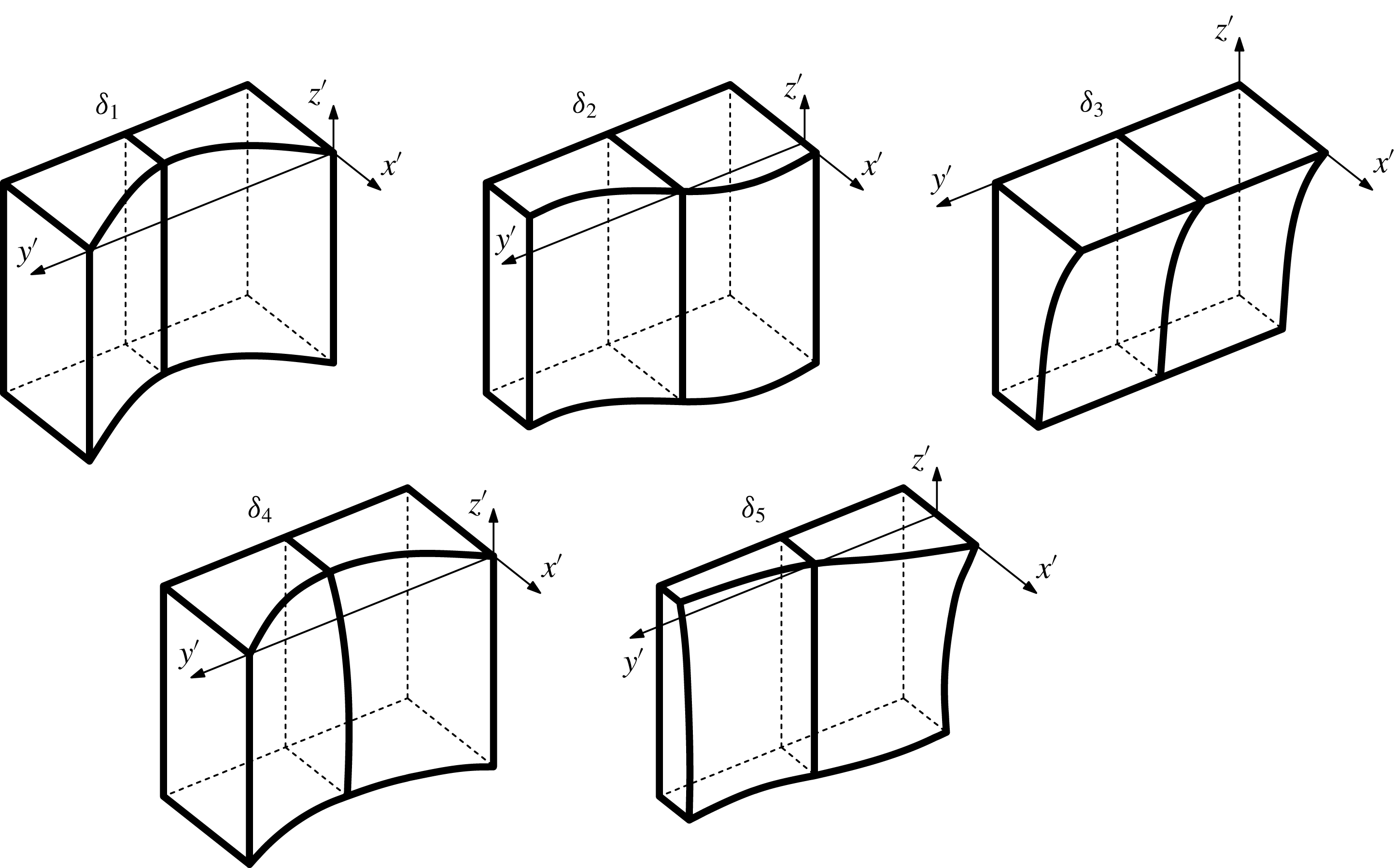
 $$\begin{eqnarray}\left.\begin{array}{@{}c@{}}\unicode[STIX]{x1D6FF}_{1}=-{\displaystyle \frac{b}{10}}\sin {\displaystyle \frac{\unicode[STIX]{x03C0}y}{b}},\quad \unicode[STIX]{x1D6FF}_{2}={\displaystyle \frac{b}{10}}\cos {\displaystyle \frac{\unicode[STIX]{x03C0}y}{b}},\quad \unicode[STIX]{x1D6FF}_{3}={\displaystyle \frac{b\cosh 0.24(h+z)}{10\cosh 0.24h}},\\ \unicode[STIX]{x1D6FF}_{4}=-{\displaystyle \frac{b\sin \displaystyle {\displaystyle \frac{\unicode[STIX]{x03C0}y}{b}}\cosh 0.24(h+z)}{10\cosh 0.24h}},\quad \unicode[STIX]{x1D6FF}_{5}={\displaystyle \frac{b\cos \displaystyle {\displaystyle \frac{\unicode[STIX]{x03C0}y}{b}}\cosh 0.24(h+z)}{10\cosh 0.24h}}.\end{array}\right\}\end{eqnarray}$$
These continuous shapes are represented in figure 2. Note that each shape is smooth and does not present irregularities that can increase significantly design costs or complicate feasibility of surging WECs in real operational conditions. Note also that configurations 1–2 depend on
 $y$
only, configuration 3 varies with the vertical
 $z$
while configurations 4–5 depend on both coordinates. The number 0.24 (in
 $\text{m}^{-1}$
) inside the expressions for
 $\unicode[STIX]{x1D6FF}_{3,4,5}$
denotes the wavenumber
 $k_{0}$
corresponding to the eigenfrequency
 $\unicode[STIX]{x1D714}=1.4~\text{rad}~\text{s}^{-1}$
. The latter value has been chosen to check whether the gates interact constructively or destructively in correspondence of that frequency. Now we investigate the effects of both synchronous and subharmonic resonance in terms of power extraction.
Sketch of the five configurations defined by expressions (5.2).

5.1 Nonlinear synchronous resonance
Let us consider the evolution equation (4.7). The values of the real coefficients
 $c_{L}$
,
 $c_{N}$
,
 $c_{R}$
,
 $c_{S}$
,
 $c_{U}$
,
 $c_{A}$
and
 $c_{B}$
with respect to the eigenfrequency
 $\unicode[STIX]{x1D714}$
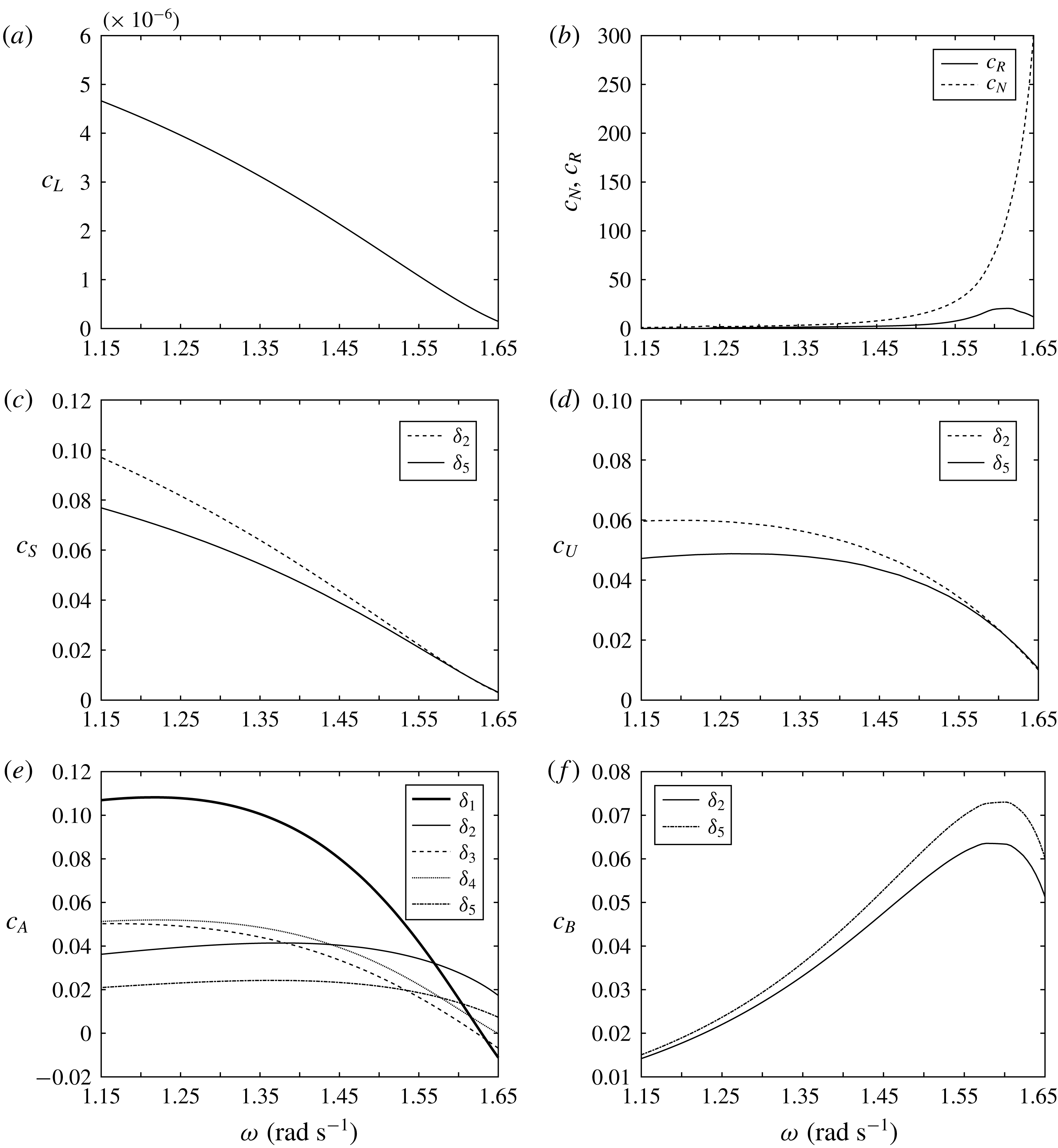
are shown in figure 3. The limiting values
 $\unicode[STIX]{x1D714}=1.15~\text{rad}~\text{s}^{-1}$
and
 $\unicode[STIX]{x1D714}=1.65~\text{rad}~\text{s}^{-1}$
correspond respectively to
 $c_{R}=0$
and the cutoff frequency at which
 $k_{0}=\unicode[STIX]{x03C0}/b$
. We remark that
 $c_{R}$
must be greater than zero because it represents damping of radiating waves (Li & Mei Reference Li and Mei2006). Figure 3(e,f) shows that
 $c_{A}$
and
 $c_{B}$
both have smooth trends without peaks or minima around
 $\unicode[STIX]{x1D714}=1.4~\text{rad}~\text{s}^{-1}$
. Therefore, contrary to intuition, matching the gate profile to the vertical eigenfunction does not give significant contributions. Sample values of the new forcing coefficients
 $c_{S}$
and
 $c_{U}$
are shown in figure 3(c,d). Symmetrical configurations about
 $y=b/2$
, i.e.
 $\unicode[STIX]{x1D6FF}_{1,3,4}$
, yield
 $c_{S}=c_{U}=0$
and cannot be resonated synchronously.
Behaviour of the coefficients of the evolution equation (4.7) versus the eigenfrequency
 $\unicode[STIX]{x1D714}$
.

Let us focus our attention on a fixed eigenfrequency and analyse the effects of the PTO damping coefficient
 $\unicode[STIX]{x1D708}=\unicode[STIX]{x1D708}_{pto}$
on the dynamic behaviour. For example, take
 $\unicode[STIX]{x1D714}=1.2~\text{rad}~\text{s}^{-1}$
and assume two values of
 $\unicode[STIX]{x1D708}_{pto}$
, respectively
 $10^{3}$
and
 $10^{4}~\text{kg}~\text{s}^{-1}$
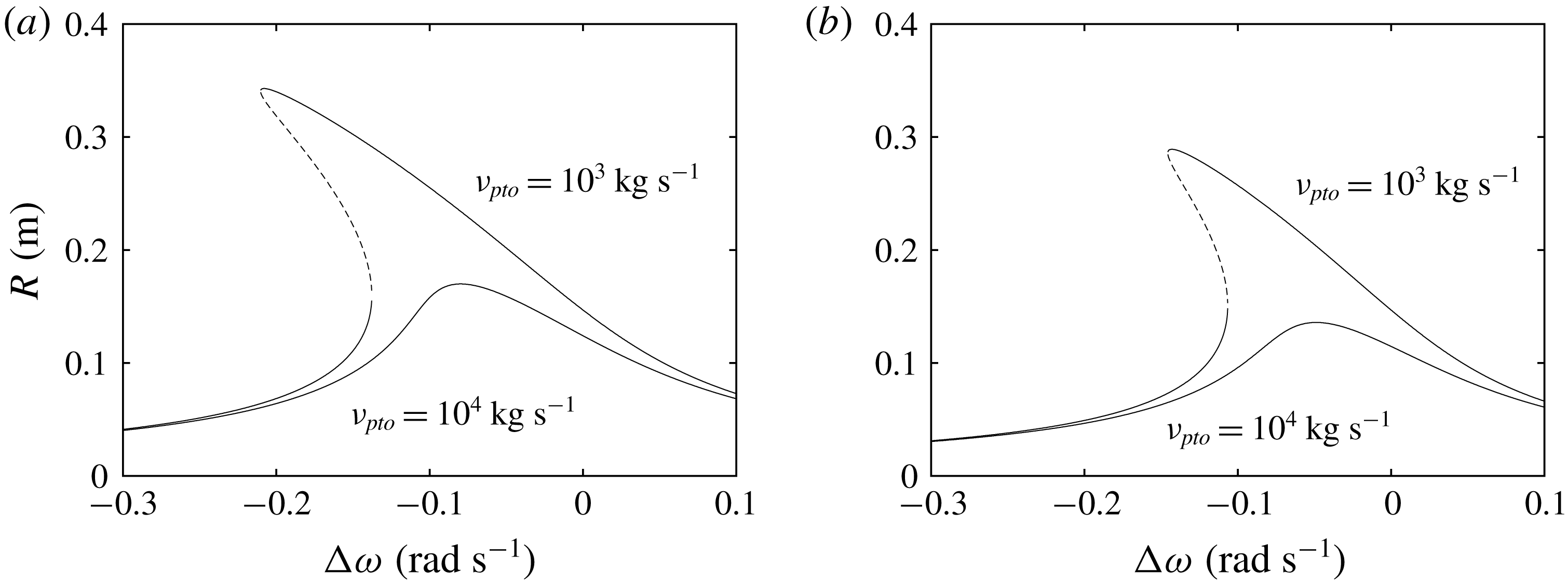
. The corresponding equilibrium branches defined by (4.13) for configurations
 $\unicode[STIX]{x1D6FF}_{2,5}$
are plotted in figure 4. The continuous lines correspond to stable fixed points, while the dashed line is related to unstable saddles (Jordan & Smith Reference Jordan and Smith2011). Note that for large values of
 $\unicode[STIX]{x1D708}_{pto}$
the unstable fixed point disappears, thus we have one stable fixed point for the entire range of detuning
 $\unicode[STIX]{x0394}\unicode[STIX]{x1D714}$
and absence of non-trivial instability.
Equilibrium branches given by (4.13) versus detuning of the incident wave
 $\unicode[STIX]{x0394}\unicode[STIX]{x1D714}$
for two different values of damping coefficient. (a) Corresponds to the shape function
 $\unicode[STIX]{x1D6FF}_{2}$
while (b) corresponds to
 $\unicode[STIX]{x1D6FF}_{5}$
. The solid lines represent the stable equilibrium branches while the dotted line represents the unstable branch. Trivial fixed points are not possible for synchronous excitation and thus the modal amplitude at the equilibrium is always positive.

Now, we evaluate the efficiency of the system excited through nonlinear synchronous interactions. The generated power by the array is given by
 $$\begin{eqnarray}P_{sync}=2\unicode[STIX]{x1D708}_{pto}(\unicode[STIX]{x1D714}+\unicode[STIX]{x0394}\unicode[STIX]{x1D714})^{2}\mathop{\sum }_{q=1}^{Q}r_{q}^{2}R^{2},\end{eqnarray}$$
thus, the capture factor (Renzi & Dias Reference Renzi and Dias2012) for synchronous resonance is
 $$\begin{eqnarray}{\mathcal{C}}_{sync}^{F}=\frac{P_{sync}}{EC_{g}b},\end{eqnarray}$$
where the term at the denominator represents the incident wave energy flux per array width
 $b$
(Michele et al.
Reference Michele, Sammarco and d’Errico2016b
), while
 $$\begin{eqnarray}EC_{g}=\frac{\unicode[STIX]{x1D70C}gA^{2}(\unicode[STIX]{x1D714}+\unicode[STIX]{x0394}\unicode[STIX]{x1D714})}{4k}\left(1+\frac{2kh}{\sinh 2kh}\right).\end{eqnarray}$$
In the latter equation, both group celerity
 $C_{g}$
and wavenumber
 $k$
are related to the frequency
 $(\unicode[STIX]{x1D714}+\unicode[STIX]{x0394}\unicode[STIX]{x1D714})$
. Figure 5 shows the maximum of
 ${\mathcal{C}}_{sync}^{F}$
for the configurations
 $\unicode[STIX]{x1D6FF}_{2,5}$
versus the eigenfrequency
 $\unicode[STIX]{x1D714}$
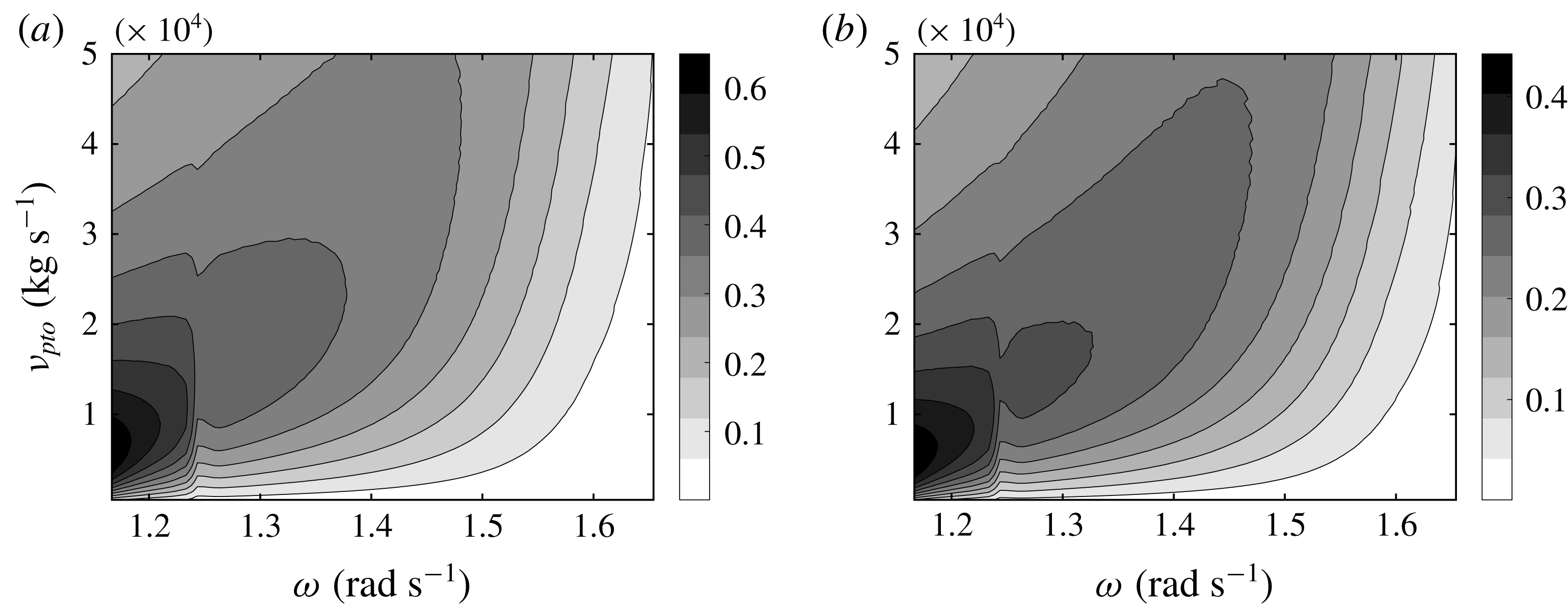
for different values of PTO coefficients. The maximum value is
 ${\sim}0.7$
for
 $\unicode[STIX]{x1D6FF}_{2}$
. This means that even in the presence of small-amplitude incident waves and trapped modes, a device designed to resonate synchronously can still achieve significant efficiency. Note that configuration
 $\unicode[STIX]{x1D6FF}_{2}$
is more efficient than
 $\unicode[STIX]{x1D6FF}_{5}$
. This can be seen from the figures 3(c) and 3(d) representing the behaviour of the forcing coefficients
 $c_{S}$
and
 $c_{U}$
, respectively. Both
 $c_{S}$
and
 $c_{U}$
for the second configuration are always greater than the coefficients for configuration 5, hence forcing contributions over
 $\unicode[STIX]{x1D6FF}_{2}$
are greater as well.
Behaviour of the maximum value of the capture factor
 ${\mathcal{C}}_{sync}^{F}$
(5.4) due to nonlinear synchronous resonance. (a) Corresponds to the shape function
 $\unicode[STIX]{x1D6FF}_{2}$
while (b) corresponds to
 $\unicode[STIX]{x1D6FF}_{5}$
.

5.2 Nonlinear subharmonic resonance
In this section we analyse the subharmonic resonance of a single trapped natural mode of an array of
 $Q$
gates. Subharmonic resonance mechanisms are already known to occur for the Venice gates (Blondeaux, Seminara & Vittori Reference Blondeaux, Seminara and Vittori1993a
,Reference Blondeaux, Seminara and Vittori
b
; Mei et al.
Reference Mei, Sammarco, Chan and Procaccini1994; Vittori et al.
Reference Vittori, Blondeaux and Seminara1996; Sammarco et al.
Reference Sammarco, Tran and Mei1997b
,Reference Sammarco, Tran, Gottlieb and Mei
a
), edge waves (Guza & Bowen Reference Guza and Bowen1976; Rockliff Reference Rockliff1978; Li Reference Li2007), cross-waves (Lichter & Chen Reference Lichter and Chen1987), Faraday waves (Miles Reference Miles1984; Holmes Reference Holmes1986; Gu & Sethna Reference Gu and Sethna1987; Miles & Henderson Reference Miles and Henderson1990) and trapped waves near a vertical cylinder in a channel (Li & Mei Reference Li and Mei2006). A similar resonance mechanism has recently been found in the context of WECs by Michele et al. (Reference Michele, Sammarco and d’Errico2018b
), but for flat gates. Here we explore the role of gate surface curvature in triggering subharmonic resonance effects. Again, the incident waves are assumed small and comparable with
 $\mathit{O}(\unicode[STIX]{x1D716})$
terms.
Let us assume a small detuning
 $2\unicode[STIX]{x0394}\unicode[STIX]{x1D714}$
between the trapped mode and the incident waves such that
 $\unicode[STIX]{x0394}\unicode[STIX]{x1D714}/\unicode[STIX]{x1D714}=\unicode[STIX]{x1D714}_{2}\unicode[STIX]{x1D716}^{2}$
(Sammarco et al.
Reference Sammarco, Tran and Mei1997b
). After some lengthy algebra, the evolution equation for subharmonic resonance is
 $$\begin{eqnarray}-\text{i}\unicode[STIX]{x1D717}_{t_{2}}=\unicode[STIX]{x1D717}(c_{A}+\text{i}c_{B})+\unicode[STIX]{x1D717}^{2}\unicode[STIX]{x1D717}^{\ast }(c_{N}+\text{i}c_{R})+A\text{e}^{-2\text{i}(\unicode[STIX]{x1D714}_{2}t_{2}+(c_{\unicode[STIX]{x1D6FF}}t_{1}/\unicode[STIX]{x1D716}))}\unicode[STIX]{x1D717}^{\ast }(c_{F}+\text{i}c_{T})+\text{i}\unicode[STIX]{x1D717}\unicode[STIX]{x1D708}c_{L},\end{eqnarray}$$
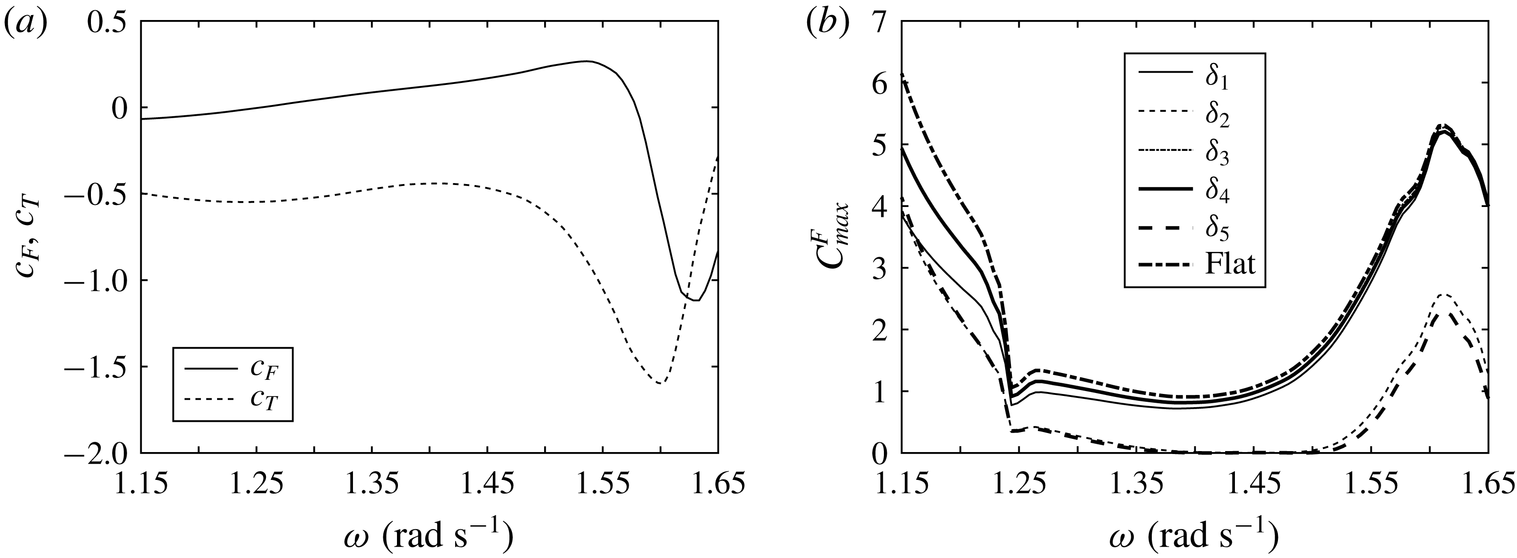
in which the behaviour of the real forcing coefficients
 $c_{F}$
,
 $c_{T}$
is represented in figure 6(a). Through the transformation
 $$\begin{eqnarray}\unicode[STIX]{x1D717}=\overline{\unicode[STIX]{x1D717}}\text{e}^{-\text{i}(\unicode[STIX]{x1D714}_{2}t_{2}+(t_{1}c_{\unicode[STIX]{x1D6FF}}/\unicode[STIX]{x1D714}\unicode[STIX]{x1D716}))},\end{eqnarray}$$
equation (5.6) becomes
 $$\begin{eqnarray}-\text{i}\overline{\unicode[STIX]{x1D717}}_{t}=\overline{\unicode[STIX]{x1D717}}(\unicode[STIX]{x0394}\unicode[STIX]{x1D714}+c_{A}+\text{i}c_{B})+\overline{\unicode[STIX]{x1D717}}^{2}\overline{\unicode[STIX]{x1D717}}^{\ast }(c_{N}+\text{i}c_{R})+A\overline{\unicode[STIX]{x1D717}}^{\ast }(c_{F}+\text{i}c_{T})+\text{i}\overline{\unicode[STIX]{x1D717}}\unicode[STIX]{x1D708}c_{L}.\end{eqnarray}$$
Equation (5.8) is similar to (4.10) and admits both trivial and non-trivial fixed points. For a detailed analysis about its properties we refer to the works of Sammarco et al. (Reference Sammarco, Tran and Mei1997b ) and Michele et al. (Reference Michele, Sammarco and d’Errico2018b ).
(a) Behaviour of the forcing coefficients
 $c_{F}$
and
 $c_{T}$
and (b) maximum of the optimal capture factor
 ${\mathcal{C}}_{max}^{F}$
versus the eigenfrequency of the array
 $\unicode[STIX]{x1D714}$
;
 ${\mathcal{C}}_{max}^{F}$
reaches values greater than 1, i.e. the maximum that can be reached with linear synchronous motion only by an asymmetric WEC.

By making use of the polar coordinates
 $R$
and
 $\unicode[STIX]{x1D713}$
(or action-angle variables) expressed by
 $\overline{\unicode[STIX]{x1D717}}=\text{i}\sqrt{R}\text{e}^{\text{i}\unicode[STIX]{x1D713}}$
, we obtain the two non-trivial fixed points with
 $R\neq 0$
:
 $$\begin{eqnarray}\displaystyle R^{\pm } & = & \displaystyle \frac{1}{c_{N}^{2}+c_{R}^{2}}\left\{\!\vphantom{\sqrt{A^{2}\left(c_{F}^{2}+c_{T}^{2}\right)\left(c_{N}^{2}+c_{R}^{2}\right)-\left[c_{N}\left(\unicode[STIX]{x1D708}c_{L}+c_{B}\right)-c_{R}\left(\unicode[STIX]{x0394}\unicode[STIX]{x1D714}+c_{A}\right)\right]^{2}}}-c_{R}(\unicode[STIX]{x1D708}c_{L}+c_{B})-c_{N}(\unicode[STIX]{x0394}\unicode[STIX]{x1D714}+c_{A})\right.\nonumber\\ \displaystyle & & \displaystyle \left.\pm \sqrt{A^{2}(c_{F}^{2}+c_{T}^{2})(c_{N}^{2}+c_{R}^{2})-[c_{N}(\unicode[STIX]{x1D708}c_{L}+c_{B})-c_{R}(\unicode[STIX]{x0394}\unicode[STIX]{x1D714}+c_{A})]^{2}}\right\}.\end{eqnarray}$$
Once the stable branch
 $R^{+}$
is evaluated (see Michele et al.
Reference Michele, Sammarco and d’Errico2018b
), the average generated power by the array due to subharmonic resonance of the natural mode is given by
 $$\begin{eqnarray}P_{sub}=2\unicode[STIX]{x1D708}(\unicode[STIX]{x1D714}+\unicode[STIX]{x0394}\unicode[STIX]{x1D714})^{2}\mathop{\sum }_{q=1}^{Q}r_{q}^{2}R^{+}.\end{eqnarray}$$
To find the maximum value of
 $P_{sub}$
we should equate to zero the partial derivatives of (5.10) with respect to
 $\unicode[STIX]{x0394}\unicode[STIX]{x1D714}$
and
 $\unicode[STIX]{x1D708}$
and then try to seek the roots of the corresponding system. However, finding an analytical expression is not possible and numerical methods are necessary. An optimum criterion can be still defined by approximating the detuning which maximises the generated power with
 $\unicode[STIX]{x0394}\unicode[STIX]{x1D714}=\unicode[STIX]{x0394}\unicode[STIX]{x1D714}_{max}$
when the gate oscillation reaches its maximum. To do so, we equate to zero the derivative of (5.10) with respect to
 $\unicode[STIX]{x1D708}$
evaluated at
 $\unicode[STIX]{x0394}\unicode[STIX]{x1D714}_{max}$
:
 $$\begin{eqnarray}\left.\frac{\text{d}P_{sub}}{\text{d}\unicode[STIX]{x1D708}}\right|_{\unicode[STIX]{x0394}\unicode[STIX]{x1D714}=\unicode[STIX]{x0394}\unicode[STIX]{x1D714}_{max}}=0.\end{eqnarray}$$
Solution of the latter equation yields
 $$\begin{eqnarray}\displaystyle \unicode[STIX]{x1D708} & = & \displaystyle \frac{1}{8c_{N}c_{L}}\left\{\vphantom{\left[\left(-9Ac_{N}\sqrt{c_{F}^{2}+c_{T}^{2}}+2c_{R}\unicode[STIX]{x1D714}\right)\right]^{1/2}}5Ac_{N}\sqrt{c_{F}^{2}+c_{T}^{2}}-5c_{B}c_{N}-2c_{R}\unicode[STIX]{x1D714}\right.\nonumber\\ \displaystyle & & \displaystyle +\left[9A^{2}c_{N}^{2}(c_{F}^{2}+c_{T}^{2})+9c_{B}^{2}c_{N}^{2}-4Ac_{N}c_{R}\unicode[STIX]{x1D714}\sqrt{c_{F}^{2}+c_{T}^{2}}+4c_{R}^{2}\unicode[STIX]{x1D714}^{2}\right.\nonumber\\ \displaystyle & & \displaystyle \left.\left.+2c_{B}c_{N}\left(-9Ac_{N}\sqrt{c_{F}^{2}+c_{T}^{2}}+2c_{R}\unicode[STIX]{x1D714}\right)\right]^{1/2}\right\}.\end{eqnarray}$$
The capture factor for subharmonic resonance
 ${\mathcal{C}}_{sub}^{F}$
becomes
 $$\begin{eqnarray}{\mathcal{C}}_{sub}^{F}=\frac{P_{sub}}{EC_{g}b},\end{eqnarray}$$
where the term at the denominator is related to the frequency
 $2(\unicode[STIX]{x1D714}+\unicode[STIX]{x0394}\unicode[STIX]{x1D714})$
.
We now define the optimal capture factor
 ${\mathcal{C}}_{max}^{F}$
as the capture factor that satisfies the optimum criterion expressed by (5.11). Figure 6(b) shows the behaviour of
 ${\mathcal{C}}_{max}^{F}$
for each configuration versus the eigenfrequency
 $\unicode[STIX]{x1D714}$
. We obtain that the flat configuration is the most efficient. This is because the coefficient
 $c_{B}$
is positive for curved anti-symmetrical shapes and generates hydrodynamic damping, which decreases efficiency. The same figure shows that the optimal capture factor is greater than 1 for a wide range of frequencies. This value corresponds to the maximum efficiency that a two-dimensional asymmetrical wave absorber can reach when excited synchronously in a linearised framework (Mei et al.
Reference Mei, Stiassnie and Yue2005). Thus, nonlinear subharmonic resonance can have beneficial effects on power extraction. Such a result confirms the previous findings of Michele et al. (Reference Michele, Sammarco and d’Errico2018b
) for flap-type WECs. However, figure 6(b) also reveals that all the curved configurations analysed here are sub-optimal with respect to a flat gate. The occurrence of the shape-dependent term
 $c_{B}$
in (5.6) has always resulted to be detrimental to the performance of the system in the case of subharmonic resonance. Therefore, our results suggest that the gate surface curvature does not increase wave power extraction when subharmonic resonance is triggered. This behaviour contrasts the positive impact that using a gate shape has in nonlinear synchronous resonance and in non-resonant states (Hodge et al.
Reference Hodge, Bateman, Yuan, Thies and Bruce2017; Michele et al.
Reference Michele, Renzi and Sammarco2018a
).
6 Conclusions
We analysed the hydrodynamic interactions between an array of curved gates and weakly nonlinear waves in a semi-infinite channel. Perturbation expansion and three timing with two slow time scales allowed us to find the complex evolution equations of the Ginzburg–Landau type both for synchronous and subharmonic excitation. New damping, detuning and forcing coefficients that are dependent on the array shape function and its derivatives appear in the equation. We remark also that this dynamics is possible only for nonlinear theories, because forcing contributions now depend on the products between the gate shape function and second-order velocity potentials at the third order.
Then we have applied the theory to the case of surge-type WECs and investigated the effects of curved shapes on the synchronous resonance mechanism by comparing a flat configuration with several curved shapes of practical engineering interest. We also demonstrated that the damping term at the third order is physically coherent with systems for power absorption. We found that effects of synchronous interactions on the generated power can be substantial for optimisation purposes. This highlights the importance of including nonlinear resonances in the cost–benefit analysis when choosing the gate shape.
We have also investigated the case of subharmonic excitation of the WEC array by normally incident waves. In all the cases analysed here, we found that the flat configuration is the most efficient for a wide range of frequencies. Several authors have recently advocated the use of curved gates to improve wave power production in non-resonant states. On the contrary, our results show that curved surfaces are usually penalised if subharmonic resonance occurs.
Finally, we point out that hydrodynamic effects such as fluid shear stresses and vortex shedding in the gap area between adjacent gates are inevitable in real conditions. These damping phenomena contribute to reduce the gate amplitude and should be considered to better evaluate the gate response and the corresponding hydrodynamics.
Acknowledgements
The work of S.M. and E.R. is supported by a Royal Society – CNR International Fellowship. Fruitful discussions with Professors B. Molin, M. Kashiwagi, P. Sclavounos and R. E. Taylor are kindly acknowledged.
Appendix A. Forcing terms and solutions of the boundary-value problems
In this appendix we derive the governing equations and the corresponding solution of each boundary-value problem with order
 $n$
and harmonic
 $m$
defined in § 3.
A.1 Leading-order problem
 $\mathit{O}(1)$
– zeroth harmonic

The forcing terms are all null:
 $$\begin{eqnarray}{\mathcal{F}}_{10}={\mathcal{B}}_{10}={\mathcal{G}}_{10}={\mathcal{D}}_{10}=0.\end{eqnarray}$$
The bounded solution is therefore independent on the fast coordinates, i.e.
 $$\begin{eqnarray}\unicode[STIX]{x1D719}_{10}=\unicode[STIX]{x1D719}_{10}(t_{1},t_{2}),\quad \unicode[STIX]{x1D712}_{10}=0,\quad \unicode[STIX]{x1D702}_{10}=0.\end{eqnarray}$$
A.2 Leading-order problem
$\mathit{O}(1)$
– first harmonic and trapped-mode solution

This problem is identical to that in Michele et al. (Reference Michele, Sammarco and d’Errico2018b ). Hereafter we recall the expression of the leading-order velocity potential
 $$\begin{eqnarray}\unicode[STIX]{x1D719}_{11}=\text{i}\unicode[STIX]{x1D712}\unicode[STIX]{x1D714}\mathop{\sum }_{q=1}^{Q}\mathop{\sum }_{m=1}^{\infty }\mathop{\sum }_{n=0}^{\infty }\frac{b_{mq}D_{n}}{C_{n}\unicode[STIX]{x1D6FC}_{nm}}\text{e}^{-\unicode[STIX]{x1D6FC}_{nm}x}\cos \frac{m\unicode[STIX]{x03C0}y}{b}\cosh k_{n}(h+z)\equiv \text{i}\unicode[STIX]{x1D712}f_{11}(x,y,z),\end{eqnarray}$$
In the latter, the terms
 $k_{n}$
are the roots of the dispersion relation
 $$\begin{eqnarray}\left.\begin{array}{@{}c@{}}\unicode[STIX]{x1D714}^{2}=gk_{0}\tanh k_{0}h,\\ \unicode[STIX]{x1D714}^{2}=-g\overline{k}_{n}\tan \overline{k}_{n}h,\quad k_{n}=\text{i}\overline{k}_{n},n=1,\ldots ,\infty .\end{array}\right\}\end{eqnarray}$$
The real coefficients in the expression for the velocity potential
 $\unicode[STIX]{x1D719}_{11}$
(A 3) are obtained by matching the velocity of the gate and of the surrounding fluid via (3.27):
 $$\begin{eqnarray}b_{mq}=r_{q}\frac{2}{m\unicode[STIX]{x03C0}}\left[\sin \frac{qm\unicode[STIX]{x03C0}}{Q}-\sin \frac{(q-1)m\unicode[STIX]{x03C0}}{Q}\right],\end{eqnarray}$$
 $$\begin{eqnarray}\unicode[STIX]{x1D6FC}_{nm}=\sqrt{\left(\frac{m\unicode[STIX]{x03C0}}{b}\right)^{2}-k_{n}^{2}},\quad C_{n}=\frac{1}{2}\left(h+\frac{g}{\unicode[STIX]{x1D714}^{2}}\sinh ^{2}k_{n}h\right),\quad D_{n}=\frac{\sinh k_{n}h}{k_{n}}.\end{eqnarray}$$
Finally, numerical solution of the equation of motion gives
 $(Q-1)$
trapped modes and related eigenfrequencies (Sammarco et al.
Reference Sammarco, Michele and d’Errico2013).
A.3 Second-order problem
$\mathit{O}(\unicode[STIX]{x1D716})$
– zeroth-harmonic drift

Combination of quadratic nonlinearities results in forcing terms of the drift flow:
 $$\begin{eqnarray}\displaystyle & \displaystyle {\mathcal{F}}_{20}=0, & \displaystyle\end{eqnarray}$$
 $$\begin{eqnarray}\displaystyle & \displaystyle {\mathcal{B}}_{20}=-\frac{\text{i}}{g\unicode[STIX]{x1D716}}[\unicode[STIX]{x1D719}_{10_{t_{1}}}\unicode[STIX]{x1D716}\unicode[STIX]{x1D714}+|\unicode[STIX]{x1D712}|^{2}(f_{11_{x}}^{2}+f_{11_{y}}^{2}-f_{11_{z}}^{2})], & \displaystyle\end{eqnarray}$$
 $$\begin{eqnarray}\displaystyle & \displaystyle {\mathcal{G}}_{20}=0, & \displaystyle\end{eqnarray}$$
 $$\begin{eqnarray}\displaystyle {\mathcal{D}}_{20} & = & \displaystyle \frac{\unicode[STIX]{x1D70C}}{\unicode[STIX]{x1D716}}\int _{(q-1)a}^{qa}\,\text{d}y\left\{\left.-\frac{\unicode[STIX]{x1D714}^{2}|\unicode[STIX]{x1D712}|^{2}}{g}f_{11}^{2}\right|_{z=0}\right.\nonumber\\ \displaystyle & & \displaystyle +\left.\int _{-h}^{0}\,\text{d}z[\unicode[STIX]{x1D719}_{10_{t_{1}}}\unicode[STIX]{x1D716}\unicode[STIX]{x1D714}+|\unicode[STIX]{x1D712}|^{2}(-f_{11_{x}}^{2}+f_{11_{y}}^{2}+f_{11_{z}}^{2})]\right\}_{x=0}.\end{eqnarray}$$
Since the forcing terms on the free surface
 ${\mathcal{F}}_{20}$
and on the gates
 ${\mathcal{G}}_{20}$
vanish, the velocity potential
 $\unicode[STIX]{x1D719}_{20}$
depends on the slow time scales in the same way as
 $\unicode[STIX]{x1D719}_{10}$
:
 $$\begin{eqnarray}\unicode[STIX]{x1D719}_{20}=\unicode[STIX]{x1D719}_{20}(t_{1},t_{2}).\end{eqnarray}$$
On the other hand, the trapped waves induce a bound wave
 $\unicode[STIX]{x1D702}_{20}$
and a static displacement
 $\unicode[STIX]{x1D712}_{q,20}$
with expressions
 $$\begin{eqnarray}\unicode[STIX]{x1D702}_{20}=-\frac{\text{i}}{g\unicode[STIX]{x1D716}}[\unicode[STIX]{x1D719}_{10_{t_{1}}}\unicode[STIX]{x1D716}\unicode[STIX]{x1D714}+|\unicode[STIX]{x1D712}|^{2}(f_{11_{x}}^{2}+f_{11_{y}}^{2}-f_{11_{z}}^{2})],\end{eqnarray}$$
 $$\begin{eqnarray}\displaystyle \unicode[STIX]{x1D712}_{q,20} & = & \displaystyle \frac{\unicode[STIX]{x1D70C}}{C\unicode[STIX]{x1D716}}\int _{(q-1)a}^{qa}\,\text{d}y\left\{\left.-\frac{\unicode[STIX]{x1D714}^{2}|\unicode[STIX]{x1D712}|^{2}}{g}f_{11}^{2}\right|_{z=0}\right.\nonumber\\ \displaystyle & & \displaystyle +\left.\int _{-h}^{0}\,\text{d}z\,[\unicode[STIX]{x1D719}_{10_{t_{1}}}\unicode[STIX]{x1D716}\unicode[STIX]{x1D714}+|\unicode[STIX]{x1D712}|^{2}(-f_{11_{x}}^{2}+f_{11_{y}}^{2}+f_{11_{z}}^{2})]\right\}_{x=0},\end{eqnarray}$$
in which the term
 $\unicode[STIX]{x1D719}_{10_{t_{1}}}$
is currently unknown and will be obtained at the third order (§ A.7).
A.4 Second-order problem
$\mathit{O}(\unicode[STIX]{x1D716})$
– first harmonic and gate shape effects

At the second order, the effects of the gate shape on the total wave field influence the first harmonic. Indeed, the forcing terms are non-null:
 $$\begin{eqnarray}\displaystyle & \displaystyle {\mathcal{F}}_{21}=-\unicode[STIX]{x1D712}_{t_{1}}\frac{2\unicode[STIX]{x1D714}^{2}f_{11}}{g}, & \displaystyle\end{eqnarray}$$
 $$\begin{eqnarray}\displaystyle & \displaystyle {\mathcal{B}}_{21}=-\unicode[STIX]{x1D712}_{t_{1}}\frac{\text{i}\unicode[STIX]{x1D714}f_{11}}{g}, & \displaystyle\end{eqnarray}$$
 $$\begin{eqnarray}\displaystyle & \displaystyle {\mathcal{G}}_{21}=r\unicode[STIX]{x1D712}_{t_{1}}\unicode[STIX]{x1D714}+\frac{\text{i}\unicode[STIX]{x1D712}}{\unicode[STIX]{x1D716}}(f_{11_{y}}\unicode[STIX]{x1D6FF}_{y}+f_{11_{z}}\unicode[STIX]{x1D6FF}_{z}-f_{11_{xx}}\unicode[STIX]{x1D6FF}), & \displaystyle\end{eqnarray}$$
 $$\begin{eqnarray}\displaystyle & \displaystyle {\mathcal{D}}_{21}=2\text{i}\unicode[STIX]{x1D714}^{2}Mr_{q}\unicode[STIX]{x1D712}_{t_{1}}+\frac{\unicode[STIX]{x1D70C}}{\unicode[STIX]{x1D716}}\int _{(q-1)a}^{qa}\,\text{d}y\int _{-h}^{0}\,\text{d}z\,[\text{i}f_{11}\unicode[STIX]{x1D712}_{t_{1}}\unicode[STIX]{x1D714}\unicode[STIX]{x1D716}+\unicode[STIX]{x1D714}f_{11_{x}}\unicode[STIX]{x1D6FF}\unicode[STIX]{x1D712}]_{x=0}. & \displaystyle\end{eqnarray}$$
Linearity allows us to decompose the velocity potential, i.e.
 $\unicode[STIX]{x1D719}_{21}=\unicode[STIX]{x1D719}_{21}^{G}+\unicode[STIX]{x1D719}_{21}^{F}$
, in which
 $\unicode[STIX]{x1D719}_{21}^{F}$
represents the solution with homogenous conditions on the gate, while
 $\unicode[STIX]{x1D719}_{21}^{G}$
is the solution with homogeneous conditions on the free surface. Both solutions can be found with the eigenfunction expansion method. After some lengthy algebra, we obtain, respectively,
 $$\begin{eqnarray}\unicode[STIX]{x1D719}_{21}^{G}=-\mathop{\sum }_{p=0}^{\infty }\mathop{\sum }_{l=0}^{\infty }\cosh k_{l}(h+z)\cos \left(\frac{p\unicode[STIX]{x03C0}y}{b}\right)\frac{\text{i}\text{e}^{\text{i}\overline{\unicode[STIX]{x1D6FC}}_{pl}x}}{\overline{\unicode[STIX]{x1D6FC}}_{pl}\unicode[STIX]{x1D716}}\left(\mathop{\sum }_{q=1}^{Q}\frac{\unicode[STIX]{x1D712}_{t_{1}}\unicode[STIX]{x1D714}\unicode[STIX]{x1D716}_{p}b_{pq}D_{l}\unicode[STIX]{x1D716}}{C_{l}}+\text{i}\unicode[STIX]{x1D712}\unicode[STIX]{x1D6E5}_{pl}\right),\end{eqnarray}$$
 $$\begin{eqnarray}\displaystyle \unicode[STIX]{x1D719}_{21}^{F} & = & \displaystyle \mathop{\sum }_{p=1}^{\infty }\mathop{\sum }_{l=0}^{\infty }\cosh k_{l}(h+z)\cos \left(\frac{p\unicode[STIX]{x03C0}y}{b}\right)\frac{2\unicode[STIX]{x1D712}_{t_{1}}\unicode[STIX]{x1D714}^{3}\cosh k_{l}h}{C_{l}g\unicode[STIX]{x1D6FC}_{pl}}\nonumber\\ \displaystyle & & \displaystyle \times \,\mathop{\sum }_{q=1}^{Q}\mathop{\sum }_{n=0}^{\infty }\frac{b_{pq}D_{n}\cosh k_{n}h(\overline{\unicode[STIX]{x1D6FC}}_{pn}\text{e}^{-x\unicode[STIX]{x1D6FC}_{pl}}-\unicode[STIX]{x1D6FC}_{pl}\text{e}^{-x\overline{\unicode[STIX]{x1D6FC}}_{pn}})}{\unicode[STIX]{x1D6FC}_{pn}C_{n}(\unicode[STIX]{x1D6FC}_{pl}^{2}-\overline{\unicode[STIX]{x1D6FC}}_{pn}^{2})},\end{eqnarray}$$
where
 $\unicode[STIX]{x1D716}_{0}=0$
and
 $\unicode[STIX]{x1D716}_{p}=1,\,p=1,\ldots ,$
while the eigenvalue
 $$\begin{eqnarray}\displaystyle \overline{\unicode[STIX]{x1D6FC}}_{pl}=\sqrt{k_{l}^{2}-\left(\frac{p\unicode[STIX]{x03C0}}{b}\right)^{2}}. & & \displaystyle\end{eqnarray}$$
The remaining term
 $\unicode[STIX]{x1D6E5}_{pl}$
is given by
 $$\begin{eqnarray}\unicode[STIX]{x1D6E5}_{pl}=\frac{1}{C_{l}\unicode[STIX]{x1D6FF}_{p}}\int _{0}^{b}\,\text{d}y\int _{-h}^{0}\cosh k_{l}(h+z)\cos \left(\frac{p\unicode[STIX]{x03C0}y}{b}\right)(-f_{11_{xx}}\unicode[STIX]{x1D6FF}+f_{11_{y}}\unicode[STIX]{x1D6FF}_{y}+f_{11_{z}}\unicode[STIX]{x1D6FF}_{z})\,\text{d}z,\end{eqnarray}$$
with
 $\unicode[STIX]{x1D6FF}_{0}=b$
and
 $\unicode[STIX]{x1D6FF}_{p}=b/2$
,
 $p=1,\ldots .$
Note that the potential
 $\unicode[STIX]{x1D719}_{21}$
is a peculiar feature of the curved geometry and does not exist for a flat array. Moreover,
 $\unicode[STIX]{x1D719}_{21}^{G}$
(A 18) includes propagating long-crested waves
 $\left(p=l=0\right)$
if the gate shape is not symmetric with respect to
 $y=b/2$
. Indeed, such long-crested component is strongly related to the gate shape and would be absent for flat configurations.
A.5 Second-order problem
$\mathit{O}(\unicode[STIX]{x1D716})$
– incident waves

The incident wave field is assumed to be at
 $\mathit{O}(\unicode[STIX]{x1D716})$
, hence the incident wave amplitude
 $A^{\prime }$
and frequency
 $\unicode[STIX]{x1D714}$
must be an order of magnitude smaller than
 $A_{T}^{\prime }$
, i.e.
 $A^{\prime }/A_{T}^{\prime }=\mathit{O}(\unicode[STIX]{x1D716})$
. The corresponding velocity potential is given by
 $$\begin{eqnarray}\unicode[STIX]{x1D719}^{I}=-\frac{\text{i}Ag}{2\unicode[STIX]{x1D716}\unicode[STIX]{x1D714}}\frac{\cosh k_{0}(h+z)}{\cosh k_{0}h}\text{e}^{-\text{i}k_{0}x},\end{eqnarray}$$
the scattering potential is
 $$\begin{eqnarray}\unicode[STIX]{x1D719}^{S}=-\frac{\text{i}Ag}{2\unicode[STIX]{x1D716}\unicode[STIX]{x1D714}}\frac{\cosh k_{0}(h+z)}{\cosh k_{0}h}\text{e}^{\text{i}k_{0}x},\end{eqnarray}$$
while the radiation potential due to the in-phase motion of the gates is given by
 $$\begin{eqnarray}\unicode[STIX]{x1D719}^{R}=-\mathop{\sum }_{l=0}^{\infty }\frac{\unicode[STIX]{x1D714}\unicode[STIX]{x1D712}^{A}D_{n}}{k_{n}C_{n}}\cosh k_{n}(h+z)\text{e}^{\text{i}k_{n}x}.\end{eqnarray}$$
The response
 $\unicode[STIX]{x1D712}^{A}$
is
 $$\begin{eqnarray}\unicode[STIX]{x1D712}^{A}=\frac{-\unicode[STIX]{x1D70C}aAgD_{0}/(\unicode[STIX]{x1D716}\cosh k_{0}h)}{-\unicode[STIX]{x1D714}^{2}M+C-\text{i}\unicode[STIX]{x1D714}^{2}\unicode[STIX]{x1D70C}a\displaystyle \mathop{\sum }_{l=0}^{\infty }{\displaystyle \frac{D_{n}^{2}}{k_{n}C_{n}}}},\end{eqnarray}$$
where the wavenumbers
 $k_{n}$
correspond the real roots of the dispersion relation (A 4).
A.6 Second-order problem
$\mathit{O}(\unicode[STIX]{x1D716})$
– radiated second harmonic

The second harmonic is forced both on the free surface and on the gate and does not depend on the shape of the gate. The forcing terms are
 $$\begin{eqnarray}\displaystyle & \displaystyle {\mathcal{F}}_{22}=-\frac{1}{\unicode[STIX]{x1D716}g}[\unicode[STIX]{x1D702}_{11}(-\unicode[STIX]{x1D714}^{2}\unicode[STIX]{x1D719}_{11_{z}}+g\unicode[STIX]{x1D719}_{11_{zz}})-2\text{i}\unicode[STIX]{x1D714}|\unicode[STIX]{x1D735}\unicode[STIX]{x1D719}_{11}|^{2}], & \displaystyle\end{eqnarray}$$
 $$\begin{eqnarray}\displaystyle & \displaystyle {\mathcal{B}}_{22}=-\frac{1}{\unicode[STIX]{x1D716}g}\left[-\text{i}\unicode[STIX]{x1D714}\unicode[STIX]{x1D719}_{11_{z}}\unicode[STIX]{x1D702}_{11}+\frac{|\unicode[STIX]{x1D735}\unicode[STIX]{x1D719}_{11}|^{2}}{2}\right], & \displaystyle\end{eqnarray}$$
 $$\begin{eqnarray}\displaystyle & \displaystyle {\mathcal{G}}_{22}=-\frac{\unicode[STIX]{x1D719}_{11_{xx}}\unicode[STIX]{x1D712}_{11}}{\unicode[STIX]{x1D716}}, & \displaystyle\end{eqnarray}$$
 $$\begin{eqnarray}\displaystyle & \displaystyle {\mathcal{D}}_{22}=\frac{\unicode[STIX]{x1D70C}}{\unicode[STIX]{x1D716}}\int _{0}^{b}\,\text{d}y\left\{\frac{g\unicode[STIX]{x1D702}_{11}^{2}}{2}-\text{i}\unicode[STIX]{x1D714}\unicode[STIX]{x1D719}_{11}\unicode[STIX]{x1D702}_{11}|_{z=0}+\int _{-h}^{0}\left(-\text{i}\unicode[STIX]{x1D714}\unicode[STIX]{x1D719}_{11_{x}}r\unicode[STIX]{x1D712}+\frac{|\unicode[STIX]{x1D735}\unicode[STIX]{x1D719}_{11}|^{2}}{2}\right)\text{d}z\right\}_{x=0}\!.\qquad & \displaystyle\end{eqnarray}$$
Similarly to the case for the first-harmonic solution at
 $\mathit{O}(\unicode[STIX]{x1D716})$
, we decompose the velocity potential as
 $\unicode[STIX]{x1D719}_{22}^{\unicode[STIX]{x1D712}}=\unicode[STIX]{x1D719}_{22}^{G}+\unicode[STIX]{x1D719}_{22}^{F}$
, where
 $\unicode[STIX]{x1D719}_{22}^{F}$
represents the solution with homogenous conditions on the gate, while
 $\unicode[STIX]{x1D719}_{22}^{G}$
is the solution with homogeneous conditions on the free surface. Again, the solution for both potentials can be obtained in terms of vertical and horizontal eigenfunction expansions:
 $$\begin{eqnarray}\displaystyle \unicode[STIX]{x1D719}_{22}^{G} & = & \displaystyle -\unicode[STIX]{x1D712}^{2}\unicode[STIX]{x1D714}\mathop{\sum }_{p=0}^{\infty }\mathop{\sum }_{l=0}^{\infty }\cosh \unicode[STIX]{x1D705}_{l}(h+z)\cos \left(\frac{p\unicode[STIX]{x03C0}y}{b}\right)\frac{\text{e}^{\text{i}\widehat{\unicode[STIX]{x1D6FC}}_{pl}x}}{\widehat{\unicode[STIX]{x1D6FC}}_{pl}}\left[\mathop{\sum }_{q=1}^{\infty }\frac{2\text{i}d_{pq}F_{l}}{E_{l}}\right.\nonumber\\ \displaystyle & & \displaystyle +\left.\frac{\unicode[STIX]{x1D6FF}_{p}}{b\unicode[STIX]{x1D716}}\mathop{\sum }_{q=1}^{Q}\mathop{\sum }_{r=1}^{Q}\mathop{\sum }_{n=0}^{\infty }\mathop{\sum }_{m=-\infty }^{\infty }\frac{b_{mq}b_{(m+p)r}\unicode[STIX]{x1D6FC}_{nm}D_{n}D_{nl}}{E_{l}C_{n}}\right],\quad m\neq 0,m+p\neq 0,\qquad\end{eqnarray}$$
 $$\begin{eqnarray}\displaystyle \unicode[STIX]{x1D719}_{22}^{F} & = & \displaystyle \frac{\text{i}\unicode[STIX]{x1D712}^{2}\unicode[STIX]{x1D714}}{4bg\unicode[STIX]{x1D716}}\mathop{\sum }_{p=0}^{\infty }\mathop{\sum }_{l=0}^{\infty }\mathop{\sum }_{q=1}^{Q}\mathop{\sum }_{r=1}^{Q}\mathop{\sum }_{n=0}^{\infty }\mathop{\sum }_{s=0}^{\infty }\mathop{\sum }_{m=-\infty }^{\infty }\cosh \unicode[STIX]{x1D705}_{l}(h+z)\cos \left(\frac{p\unicode[STIX]{x03C0}y}{b}\right)\cosh k_{n}h\cosh k_{s}h\nonumber\\ \displaystyle & & \displaystyle \times \,\frac{\unicode[STIX]{x1D6FF}_{p}\unicode[STIX]{x1D6FD}_{qnm}\unicode[STIX]{x1D6FD}_{r(m+p)s}\cosh \unicode[STIX]{x1D705}_{l}h[\widehat{\unicode[STIX]{x1D6FC}}_{pl}\text{e}^{-x(\unicode[STIX]{x1D6FC}_{nm}+\unicode[STIX]{x1D6FC}_{(m+p)s})}-\text{i}(\unicode[STIX]{x1D6FC}_{nm}+\unicode[STIX]{x1D6FC}_{(m+p)s})\text{e}^{\text{i}\widehat{\unicode[STIX]{x1D6FC}}_{pl}x}]}{E_{l}[\widehat{\unicode[STIX]{x1D6FC}}_{pl}^{2}+(\unicode[STIX]{x1D6FC}_{nm}+\unicode[STIX]{x1D6FC}_{(m+p)s})^{2}]}\nonumber\\ \displaystyle & & \displaystyle \times \,\left(\frac{3\unicode[STIX]{x1D714}^{4}}{g^{2}}-k_{n}^{2}+\frac{2m\unicode[STIX]{x03C0}(m+p)}{b^{2}}+2\unicode[STIX]{x1D6FC}_{nm}\unicode[STIX]{x1D6FC}_{(m+p)s}\right),\quad m\neq 0,m+p\neq 0,\end{eqnarray}$$
where
 $$\begin{eqnarray}\displaystyle D_{nl}=\frac{\unicode[STIX]{x1D705}_{l}\cosh k_{n}h\sinh \unicode[STIX]{x1D705}_{l}h-k_{n}\cosh \unicode[STIX]{x1D705}_{l}h\sinh k_{n}h}{\unicode[STIX]{x1D705}_{l}^{2}-k_{n}^{2}}, & & \displaystyle\end{eqnarray}$$
 $$\begin{eqnarray}\displaystyle \unicode[STIX]{x1D6FD}_{qnm}=\frac{\unicode[STIX]{x1D714}b_{mq}D_{n}}{\unicode[STIX]{x1D6FC}_{nm}C_{n}},\quad \widehat{\unicode[STIX]{x1D6FC}}_{pl}=\sqrt{\unicode[STIX]{x1D705}_{l}^{2}-\left(\frac{p\unicode[STIX]{x03C0}}{b}\right)^{2}}. & & \displaystyle\end{eqnarray}$$
The term
 $d_{pq}$
corresponds to the Fourier coefficient for the gate displacement:
 $$\begin{eqnarray}\displaystyle d_{pq}=\unicode[STIX]{x1D712}_{q,22}\frac{2}{p\unicode[STIX]{x03C0}}\left[\sin \frac{qp\unicode[STIX]{x03C0}}{Q}-\sin \frac{(q-1)p\unicode[STIX]{x03C0}}{Q}\right], & & \displaystyle\end{eqnarray}$$
in which
 $\unicode[STIX]{x1D712}_{q,22}$
denotes the displacement of the
 $q$
th gate normalised with respect to
 $\text{i}\unicode[STIX]{x1D712}^{2}$
. Unlike the case of Sammarco et al. (Reference Sammarco, Tran and Mei1997b
), the forcing term
 ${\mathcal{D}}_{22}$
given by (A 29) does not vanish, hence the displacement related to the second harmonic differs from zero. Indeed, usage of the equation of motion (3.28) gives a forced linear system for the unknowns
 $\unicode[STIX]{x1D712}_{q,22}$
,
 $q=1,\ldots ,Q$
. The corresponding determinant of the coefficient matrix differs from zero, thus the inhomogeneous solution is unique. After some algebra we obtain
 $$\begin{eqnarray}\displaystyle & & \displaystyle \unicode[STIX]{x1D712}_{j,22}(-4\unicode[STIX]{x1D714}^{2}M+C)-4\text{i}\unicode[STIX]{x1D714}^{2}\unicode[STIX]{x1D70C}\mathop{\sum }_{q=1}^{Q}\mathop{\sum }_{p=0}^{\infty }\mathop{\sum }_{l=0}^{\infty }\frac{d_{pq}c_{pj}F_{l}^{2}}{\widehat{\unicode[STIX]{x1D6FC}}_{pl}E_{l}}\nonumber\\ \displaystyle & & \displaystyle \quad =\frac{\unicode[STIX]{x1D70C}}{\unicode[STIX]{x1D716}}\left\{-\frac{\text{i}\unicode[STIX]{x1D714}\unicode[STIX]{x1D6FF}_{p}}{2b}\mathop{\sum }_{p=0}^{\infty }\mathop{\sum }_{l=0}^{\infty }\mathop{\sum }_{q=1}^{Q}\mathop{\sum }_{r=1}^{Q}\mathop{\sum }_{n=0}^{\infty }\mathop{\sum }_{s=0}^{\infty }\mathop{\sum }_{m=-\infty }^{\infty }\right.\nonumber\\ \displaystyle & & \displaystyle \qquad \times \,\left(\frac{3\unicode[STIX]{x1D714}^{4}}{g^{2}}-k_{n}^{2}+\frac{2m\unicode[STIX]{x03C0}(m+p)}{b^{2}}+2\unicode[STIX]{x1D6FC}_{nm}\unicode[STIX]{x1D6FC}_{(m+p)s}\right)\nonumber\\ \displaystyle & & \displaystyle \qquad \times \,\frac{\unicode[STIX]{x1D714}F_{l}c_{pj}\unicode[STIX]{x1D6FD}_{qnm}\unicode[STIX]{x1D6FD}_{r(m+p)s}\cosh \unicode[STIX]{x1D705}_{l}h[\widehat{\unicode[STIX]{x1D6FC}}_{pl}-\text{i}(\unicode[STIX]{x1D6FC}_{nm}+\unicode[STIX]{x1D6FC}_{(m+p)s})]}{g\widehat{\unicode[STIX]{x1D6FC}}_{pl}E_{l}[\widehat{\unicode[STIX]{x1D6FC}}_{pl}^{2}+(\unicode[STIX]{x1D6FC}_{nm}+\unicode[STIX]{x1D6FC}_{(m+p)s})^{2}]}\nonumber\\ \displaystyle & & \displaystyle \qquad +\,\mathop{\sum }_{p=0}^{\infty }\mathop{\sum }_{l=0}^{\infty }\mathop{\sum }_{q=1}^{Q}\mathop{\sum }_{r=1}^{Q}\mathop{\sum }_{n=0}^{\infty }\mathop{\sum }_{m=-\infty }^{\infty }\frac{\text{i}\unicode[STIX]{x1D714}c_{pj}b_{mq}b_{(m+p)r}\unicode[STIX]{x1D6FC}_{nm}F_{l}D_{n}D_{nl}}{\unicode[STIX]{x1D6FC}_{nm}\widehat{\unicode[STIX]{x1D6FC}}_{pl}E_{l}C_{n}}\nonumber\\ \displaystyle & & \displaystyle \qquad +\left.\text{i}\left(\frac{3ah\unicode[STIX]{x1D714}^{2}r_{j}^{2}}{2}+\int _{(q-1)a}^{qa}\,\text{d}y\int _{-h}^{0}\frac{f_{11_{z}}^{2}+f_{11_{y}}^{2}}{2}\,\text{d}z+\int _{(q-1)a}^{qa}\frac{\unicode[STIX]{x1D714}^{2}f_{11}^{2}}{2g}\,\text{d}y\right)\right\}\!,\qquad\end{eqnarray}$$
where the term
 $c_{pj}$
is given by
 $$\begin{eqnarray}c_{pj}=\frac{b}{p\unicode[STIX]{x03C0}}\left[\sin \frac{jp\unicode[STIX]{x03C0}}{Q}-\sin \frac{(j-1)p\unicode[STIX]{x03C0}}{Q}\right].\end{eqnarray}$$
A.7 The third-order problem
$\mathit{O}(\unicode[STIX]{x1D716}^{2})$
– zeroth harmonic

For the zeroth harmonic at
 $\mathit{O}(\unicode[STIX]{x1D716}^{2})$
the forcing terms respectively on the free surface and on the gate are
 $$\begin{eqnarray}\displaystyle {\mathcal{F}}_{30} & = & \displaystyle -\unicode[STIX]{x1D714}^{2}\unicode[STIX]{x1D719}_{10_{t_{1}t_{1}}}+\frac{1}{g\unicode[STIX]{x1D716}}\left\{\frac{3\unicode[STIX]{x1D714}^{4}f_{11}\unicode[STIX]{x1D714}(\unicode[STIX]{x1D712}\unicode[STIX]{x1D712}_{t_{1}}^{\ast }+\unicode[STIX]{x1D712}^{\ast }\unicode[STIX]{x1D712}_{t_{1}})}{g}+\unicode[STIX]{x1D714}f_{11}(\unicode[STIX]{x1D712}^{\ast }\unicode[STIX]{x1D719}_{21_{zz}}+\unicode[STIX]{x1D712}\unicode[STIX]{x1D719}_{21_{zz}}^{\ast })\right.\nonumber\\ \displaystyle & & \displaystyle -\left.2\unicode[STIX]{x1D714}|\unicode[STIX]{x1D712}|_{t_{1}}^{2}|\unicode[STIX]{x1D735}f_{11}|^{2}+\unicode[STIX]{x1D714}f_{11_{z}}[\unicode[STIX]{x1D712}^{\ast }(-\unicode[STIX]{x1D719}_{21}+\unicode[STIX]{x1D712}_{t_{1}}f_{11})-\unicode[STIX]{x1D712}(\unicode[STIX]{x1D719}_{21}^{\ast }+\unicode[STIX]{x1D712}_{t_{1}}^{\ast }f_{11})]\vphantom{\frac{3\unicode[STIX]{x1D714}^{4}f_{11}\unicode[STIX]{x1D714}(\unicode[STIX]{x1D712}\unicode[STIX]{x1D712}_{t_{1}}^{\ast }+\unicode[STIX]{x1D712}^{\ast }\unicode[STIX]{x1D712}_{t_{1}})}{g}}\right\},\end{eqnarray}$$
 $$\begin{eqnarray}\displaystyle {\mathcal{G}}_{30}=-\frac{r}{\unicode[STIX]{x1D716}}(\unicode[STIX]{x1D712}^{\ast }\unicode[STIX]{x1D719}_{21_{xx}}+\unicode[STIX]{x1D712}\unicode[STIX]{x1D719}_{21_{xx}}^{\ast })+\unicode[STIX]{x1D714}\unicode[STIX]{x1D712}_{20_{t_{1}}}. & & \displaystyle\end{eqnarray}$$
Note that the dependence of
 $\unicode[STIX]{x1D719}_{10}$
(A 2) on the slow time coordinate
 $t_{1}$
is still unknown. Application of Green’s theorem to
 $\unicode[STIX]{x1D719}_{10}$
and
 $\unicode[STIX]{x1D719}_{30}$
yields
 $$\begin{eqnarray}-\int _{0}^{b}\,\text{d}y\int _{0}^{X}{\mathcal{F}}_{30}|_{z=0}\,\text{d}x+\int _{0}^{b}\,\text{d}y\int _{-h}^{0}{\mathcal{G}}_{30}|_{x=0}\,\text{d}z-\int _{0}^{b}\,\text{d}y\int _{-h}^{0}\unicode[STIX]{x1D719}_{10}\unicode[STIX]{x1D719}_{30_{x}}|_{x=X}\,\text{d}z=0,\end{eqnarray}$$
where
 $X\gg 1$
corresponds to a large value of the
 $x$
-coordinate. Solving the integrals and requesting that
 $\left|\unicode[STIX]{x1D735}\unicode[STIX]{x1D719}_{30}\right|\rightarrow 0$
as
 $X\rightarrow +\infty$
, we obtain
 $$\begin{eqnarray}\unicode[STIX]{x1D719}_{10_{t_{1}t_{1}}}=0,\end{eqnarray}$$
in the limit
 $X\rightarrow +\infty$
. Therefore, the bounded non-secular solution of (A 40) is simply
 $\unicode[STIX]{x1D719}_{10}=0$
.
A.8 The third-order problem
$\mathit{O}(\unicode[STIX]{x1D716}^{2})$
– first harmonic and forcing terms

The forcing terms
 ${\mathcal{F}}_{31}$
,
 ${\mathcal{G}}_{31}$
and
 ${\mathcal{D}}_{31}$
are given by the following expressions:
 $$\begin{eqnarray}\displaystyle {\mathcal{F}}_{31} & = & \displaystyle \frac{\unicode[STIX]{x1D714}^{2}}{g}(2\text{i}\unicode[STIX]{x1D719}_{21_{t_{1}}}-2\unicode[STIX]{x1D712}_{t_{2}}-f_{11}\unicode[STIX]{x1D712}_{t_{1}t_{1}})+\frac{1}{g\unicode[STIX]{x1D716}}\left\{\vphantom{\left[-2\text{i}\unicode[STIX]{x1D714}\unicode[STIX]{x1D719}_{22}-\frac{\unicode[STIX]{x1D712}^{2}}{\unicode[STIX]{x1D716}}\left(\frac{3f_{11_{z}}^{2}}{2}+\frac{f_{11_{x}}^{2}+f_{11_{y}}^{2}}{2}\right)\right]}\frac{\unicode[STIX]{x1D714}f_{11}\unicode[STIX]{x1D712}^{\ast }}{g}(-4\unicode[STIX]{x1D714}^{2}\unicode[STIX]{x1D719}_{22_{z}}+g\unicode[STIX]{x1D719}_{22_{zz}})\right.\nonumber\\ \displaystyle & & \displaystyle +\,\frac{\text{i}\unicode[STIX]{x1D712}^{\ast }}{g}\left[-2\text{i}\unicode[STIX]{x1D714}\unicode[STIX]{x1D719}_{22}-\frac{\unicode[STIX]{x1D712}^{2}}{\unicode[STIX]{x1D716}}\left(\frac{3f_{11_{z}}^{2}}{2}+\frac{f_{11_{x}}^{2}+f_{11_{y}}^{2}}{2}\right)\right](\unicode[STIX]{x1D714}^{2}f_{11_{z}}-gf_{11_{z}})\nonumber\\ \displaystyle & & \displaystyle -\,\frac{\text{i}\unicode[STIX]{x1D714}^{2}f_{11}^{2}\unicode[STIX]{x1D712}|\unicode[STIX]{x1D712}|^{2}}{2\unicode[STIX]{x1D716}g^{2}}(-\unicode[STIX]{x1D714}^{2}f_{11_{zz}}+gf_{11_{zzz}})+2\unicode[STIX]{x1D714}\unicode[STIX]{x1D712}^{\ast }(\unicode[STIX]{x1D735}f_{11}\boldsymbol{\cdot }\unicode[STIX]{x1D735}\unicode[STIX]{x1D719}_{22})\nonumber\\ \displaystyle & & \displaystyle +\,\frac{2\text{i}\unicode[STIX]{x1D714}^{2}\unicode[STIX]{x1D712}|\unicode[STIX]{x1D712}|^{2}f_{11}|\unicode[STIX]{x1D735}f_{11}|_{z}^{2}}{\unicode[STIX]{x1D716}g}-\frac{3\text{i}\unicode[STIX]{x1D712}|\unicode[STIX]{x1D712}|^{2}\unicode[STIX]{x1D735}f_{11}\boldsymbol{\cdot }\unicode[STIX]{x1D735}|\unicode[STIX]{x1D735}f_{11}|^{2}}{2\unicode[STIX]{x1D716}}\nonumber\\ \displaystyle & & \displaystyle -\left.\frac{\unicode[STIX]{x1D712}|\unicode[STIX]{x1D712}|^{2}}{g\unicode[STIX]{x1D716}}(f_{11_{x}}^{2}+f_{11_{y}}^{2}-f_{11_{z}}^{2})(-\unicode[STIX]{x1D714}^{2}f_{11_{z}}+gf_{11_{zz}})\vphantom{\left[-2\text{i}\unicode[STIX]{x1D714}\unicode[STIX]{x1D719}_{22}-\frac{\unicode[STIX]{x1D712}^{2}}{\unicode[STIX]{x1D716}}\left(\frac{3f_{11_{z}}^{2}}{2}+\frac{f_{11_{x}}^{2}+f_{11_{y}}^{2}}{2}\right)\right]}\right\},\end{eqnarray}$$
 $$\begin{eqnarray}\displaystyle {\mathcal{G}}_{31} & = & \displaystyle r\unicode[STIX]{x1D714}\unicode[STIX]{x1D712}_{t_{2}}+\frac{1}{\unicode[STIX]{x1D716}}\left\{-\unicode[STIX]{x1D712}|\unicode[STIX]{x1D712}|^{2}f_{11_{xx}}\unicode[STIX]{x1D712}_{q,22}-\unicode[STIX]{x1D712}^{\ast }r\unicode[STIX]{x1D719}_{22_{xx}}-\unicode[STIX]{x1D719}_{21_{xx}}\unicode[STIX]{x1D6FF}-\frac{\unicode[STIX]{x1D712}|\unicode[STIX]{x1D712}|^{2}f_{11_{xxx}}r}{2\unicode[STIX]{x1D716}}\right.\nonumber\\ \displaystyle & & \displaystyle -\left.\frac{\text{i}\unicode[STIX]{x1D712}f_{11_{xxx}}\unicode[STIX]{x1D6FF}^{2}}{2\unicode[STIX]{x1D716}}+\unicode[STIX]{x1D719}_{21_{y}}\unicode[STIX]{x1D6FF}_{y}+\unicode[STIX]{x1D719}_{21_{z}}\unicode[STIX]{x1D6FF}_{z}+\frac{\text{i}\unicode[STIX]{x1D712}\unicode[STIX]{x1D6FF}}{\unicode[STIX]{x1D716}}(f_{11_{xy}}\unicode[STIX]{x1D6FF}_{y}+f_{11_{xz}}\unicode[STIX]{x1D6FF}_{z})\right\},\end{eqnarray}$$
 $$\begin{eqnarray}\displaystyle {\mathcal{D}}_{31} & = & \displaystyle \frac{\unicode[STIX]{x1D70C}}{\unicode[STIX]{x1D716}}\int _{(q-1)a}^{qa}\,\text{d}y\int _{-h}^{0}\,\text{d}z\left\{\text{i}\unicode[STIX]{x1D716}\unicode[STIX]{x1D714}\unicode[STIX]{x1D712}_{t_{2}}f_{11}+\unicode[STIX]{x1D716}\unicode[STIX]{x1D714}\unicode[STIX]{x1D719}_{21_{t_{1}}}-\text{i}\unicode[STIX]{x1D714}\unicode[STIX]{x1D6FF}\unicode[STIX]{x1D719}_{21_{x}}+\text{i}\unicode[STIX]{x1D716}\unicode[STIX]{x1D714}\unicode[STIX]{x1D712}_{t_{1}}f_{11_{x}}\unicode[STIX]{x1D6FF}-\frac{\unicode[STIX]{x1D714}^{2}r\unicode[STIX]{x1D712}\unicode[STIX]{x1D712}_{20}}{\unicode[STIX]{x1D716}}\right.\nonumber\\ \displaystyle & & \displaystyle +\,\text{i}\unicode[STIX]{x1D712}|\unicode[STIX]{x1D712}|^{2}f_{11_{x}}\unicode[STIX]{x1D712}_{q,22}+\frac{\unicode[STIX]{x1D712}}{2\unicode[STIX]{x1D716}}(3|\unicode[STIX]{x1D712}|^{2}f_{11_{xx}}\unicode[STIX]{x1D714}r_{q}^{2}+f_{11_{xx}}\unicode[STIX]{x1D714}\unicode[STIX]{x1D6FF}^{2}+|\unicode[STIX]{x1D712}|^{2}r_{q}|\unicode[STIX]{x1D735}f_{11}|_{x}^{2})\nonumber\\ \displaystyle & & \displaystyle -\left.\text{i}\unicode[STIX]{x1D712}^{\ast }\unicode[STIX]{x1D735}f_{11}\boldsymbol{\cdot }\unicode[STIX]{x1D735}\unicode[STIX]{x1D719}_{22}\vphantom{\frac{\unicode[STIX]{x1D714}^{2}r\unicode[STIX]{x1D712}\unicode[STIX]{x1D712}_{20}}{\unicode[STIX]{x1D716}}}\right\}_{x=0}+\frac{\unicode[STIX]{x1D70C}}{\unicode[STIX]{x1D716}}\int _{(q-1)a}^{qa}\,\text{d}y\left\{\frac{2\text{i}\unicode[STIX]{x1D714}^{2}f_{11}\unicode[STIX]{x1D719}_{22}}{g}+\frac{3\unicode[STIX]{x1D712}|\unicode[STIX]{x1D712}|^{2}f_{11_{z}}f_{11}^{2}\unicode[STIX]{x1D714}^{3}}{2g^{2}\unicode[STIX]{x1D716}}\right.\nonumber\\ \displaystyle & & \displaystyle -\left.\frac{\unicode[STIX]{x1D712}|\unicode[STIX]{x1D712}|^{2}f_{11}\unicode[STIX]{x1D714}}{2g\unicode[STIX]{x1D716}}(6f_{11_{x}}\unicode[STIX]{x1D714}+|\unicode[STIX]{x1D735}f_{11}|^{2})\right\}_{x=0,z=0}-M\unicode[STIX]{x1D714}^{2}(-2\text{i}\unicode[STIX]{x1D712}_{t_{2}}+\unicode[STIX]{x1D712}_{t_{1}t_{1}})+\frac{\text{i}r_{q}\unicode[STIX]{x1D714}\unicode[STIX]{x1D708}\unicode[STIX]{x1D712}}{\unicode[STIX]{x1D716}^{2}}.\nonumber\\ \displaystyle & & \displaystyle\end{eqnarray}$$
Appendix B. Expressions for the coefficient of the evolution equations (4.10) and (5.8)
Let us decompose
 $\unicode[STIX]{x1D719}_{21}$
as follows:
 $$\begin{eqnarray}\unicode[STIX]{x1D719}_{21}=\unicode[STIX]{x1D712}_{t_{1}}\frac{\unicode[STIX]{x1D719}_{21}^{(1)}}{\unicode[STIX]{x1D716}}+\unicode[STIX]{x1D712}\frac{\unicode[STIX]{x1D719}_{21}^{(2)}}{\unicode[STIX]{x1D716}}.\end{eqnarray}$$
The expressions for the synchronous forcing coefficients are
 $$\begin{eqnarray}c_{S}=\text{Re}\left\{\frac{\text{i}\unicode[STIX]{x1D708}^{S}}{\widehat{\unicode[STIX]{x1D708}}}\right\},\quad c_{U}=\text{Im}\left\{\frac{\text{i}\unicode[STIX]{x1D708}^{S}}{\widehat{\unicode[STIX]{x1D708}}}\right\},\end{eqnarray}$$
with
 $$\begin{eqnarray}\displaystyle \unicode[STIX]{x1D708}^{S}=\int _{0}^{b}\,\text{d}y\int _{-h}^{0}\{f_{11}(\unicode[STIX]{x1D719}_{xx}^{A}\unicode[STIX]{x1D6FF}-\unicode[STIX]{x1D719}_{z}^{A}\unicode[STIX]{x1D6FF}_{z})+r\unicode[STIX]{x1D714}\unicode[STIX]{x1D6FF}\unicode[STIX]{x1D719}_{x}^{A}\}\,\text{d}z. & & \displaystyle\end{eqnarray}$$
In the latter, the velocity potential
 $\unicode[STIX]{x1D719}^{A}=\unicode[STIX]{x1D719}^{I}+\unicode[STIX]{x1D719}^{S}+\unicode[STIX]{x1D719}^{R}$
refers to the first-harmonic incident, scattered and in-phase radiation potentials (A 22)–(A 24). The expressions for the remaining coefficients inside the evolution equations (4.10)–(5.8) are
 $$\begin{eqnarray}c_{A}=\text{Re}\left\{\frac{\text{i}}{\widehat{\unicode[STIX]{x1D708}}}(\unicode[STIX]{x1D708}+\text{i}c_{\unicode[STIX]{x1D6FF}}\widetilde{\unicode[STIX]{x1D708}}-c_{\unicode[STIX]{x1D6FF}}^{2}\overline{\unicode[STIX]{x1D708}})\right\},\quad c_{B}=\text{Im}\left\{\frac{\text{i}}{\widehat{\unicode[STIX]{x1D708}}}(\unicode[STIX]{x1D708}+\text{i}c_{\unicode[STIX]{x1D6FF}}\widetilde{\unicode[STIX]{x1D708}}-c_{\unicode[STIX]{x1D6FF}}^{2}\overline{\unicode[STIX]{x1D708}})\right\},\end{eqnarray}$$
 $$\begin{eqnarray}c_{N}=\text{Re}\left\{\frac{\text{i}\unicode[STIX]{x1D708}^{R}}{\widehat{\unicode[STIX]{x1D708}}}\right\},\quad c_{R}=\text{Im}\left\{\frac{\text{i}\unicode[STIX]{x1D708}^{R}}{\widehat{\unicode[STIX]{x1D708}}}\right\},\quad c_{F}=\text{Re}\left\{\frac{\text{i}\unicode[STIX]{x1D708}^{I}}{\widehat{\unicode[STIX]{x1D708}}}\right\},\quad c_{T}=\text{Im}\left\{\frac{\text{i}\unicode[STIX]{x1D708}^{I}}{\widehat{\unicode[STIX]{x1D708}}}\right\},\end{eqnarray}$$
 $$\begin{eqnarray}c_{L}=-\frac{\text{i}}{\widehat{\unicode[STIX]{x1D708}}}\mathop{\sum }_{q=1}^{Q}\frac{\unicode[STIX]{x1D714}r_{q}^{2}}{\unicode[STIX]{x1D70C}},\end{eqnarray}$$
where
 $$\begin{eqnarray}\widehat{\unicode[STIX]{x1D708}}=-\int _{0}^{b}\,\text{d}y\int _{0}^{+\infty }\frac{2f_{11}^{2}\unicode[STIX]{x1D714}}{g}\,\text{d}x-\int _{0}^{b}\,\text{d}y\int _{-h}^{0}2f_{11}r\,\text{d}z-\mathop{\sum }_{q=1}^{Q}\frac{2r^{2}\unicode[STIX]{x1D714}M}{\unicode[STIX]{x1D70C}},\end{eqnarray}$$
 $$\begin{eqnarray}\displaystyle \unicode[STIX]{x1D708} & = & \displaystyle \int _{0}^{b}\,\text{d}y\int _{-h}^{0}\,\text{d}z\left\{-f_{11}\left[-\unicode[STIX]{x1D6FF}\unicode[STIX]{x1D719}_{21_{xx}}^{(2)}+\unicode[STIX]{x1D6FF}_{y}\unicode[STIX]{x1D719}_{21_{y}}^{(2)}+\unicode[STIX]{x1D6FF}_{z}\unicode[STIX]{x1D719}_{21_{z}}^{(2)}-\frac{\text{i}\unicode[STIX]{x1D6FF}^{2}f_{11_{xxx}}}{2}\right.\right.\nonumber\\ \displaystyle & & \displaystyle +\left.\left.\text{i}\unicode[STIX]{x1D6FF}(f_{11_{xy}}\unicode[STIX]{x1D6FF}_{y}+f_{11_{xz}}\unicode[STIX]{x1D6FF}_{z})\vphantom{\frac{\text{i}\unicode[STIX]{x1D6FF}^{2}f_{11_{xxx}}}{2}}\right]+\text{i}r\unicode[STIX]{x1D6FF}\unicode[STIX]{x1D714}\left(-\frac{\unicode[STIX]{x1D6FF}f_{11_{xx}}}{2}+f_{11_{y}}\unicode[STIX]{x1D6FF}_{y}+f_{11_{z}}\unicode[STIX]{x1D6FF}_{z}\right)\right\},\end{eqnarray}$$
 $$\begin{eqnarray}\displaystyle \widetilde{\unicode[STIX]{x1D708}} & = & \displaystyle \int _{0}^{b}\,\text{d}y\int _{0}^{+\infty }\frac{2\text{i}f_{11}\unicode[STIX]{x1D719}_{21}^{(2)}\unicode[STIX]{x1D714}}{g}\,\text{d}x+\int _{0}^{b}\,\text{d}y\int _{-h}^{0}\,\text{d}z\{-f_{11}[-\unicode[STIX]{x1D6FF}\unicode[STIX]{x1D719}_{21_{xx}}^{(1)}+\unicode[STIX]{x1D6FF}_{y}\unicode[STIX]{x1D719}_{21_{y}}^{(1)}+\unicode[STIX]{x1D6FF}_{z}\unicode[STIX]{x1D719}_{21_{z}}^{(1)}]\nonumber\\ \displaystyle & & \displaystyle +\,\text{i}r(-2\text{i}\unicode[STIX]{x1D6FF}\unicode[STIX]{x1D714}r+\unicode[STIX]{x1D719}_{21}^{(2)})\!\},\end{eqnarray}$$
 $$\begin{eqnarray}\overline{\unicode[STIX]{x1D708}}=\int _{0}^{b}\,\text{d}y\int _{0}^{+\infty }\frac{2\text{i}f_{11}\unicode[STIX]{x1D719}_{21}^{(1)}\unicode[STIX]{x1D714}-\text{i}f_{11}^{2}}{g}\,\text{d}x+\int _{0}^{b}\,\text{d}y\int _{-h}^{0}\text{i}r\unicode[STIX]{x1D719}_{21}^{(1)}\,\text{d}z+\mathop{\sum }_{q=1}^{Q}\frac{\text{i}Mr_{q}^{2}}{\unicode[STIX]{x1D70C}},\end{eqnarray}$$
 $$\begin{eqnarray}\displaystyle \unicode[STIX]{x1D708}^{I} & = & \displaystyle \int _{0}^{b}\,\text{d}y\int _{0}^{+\infty }f_{11}\left\{\frac{f_{11}\unicode[STIX]{x1D714}}{g}(-4\unicode[STIX]{x1D714}^{2}\tilde{\unicode[STIX]{x1D719}}_{z}^{A}+g\tilde{\unicode[STIX]{x1D719}}_{zz}^{A})+\frac{2\unicode[STIX]{x1D714}\tilde{\unicode[STIX]{x1D719}}^{A}}{g}(\unicode[STIX]{x1D714}^{2}f_{11_{z}}-gf_{11_{zz}})\right.\nonumber\\ \displaystyle & & \displaystyle +\left.2\unicode[STIX]{x1D714}\unicode[STIX]{x1D735}f_{11}\boldsymbol{\cdot }\unicode[STIX]{x1D735}\tilde{\unicode[STIX]{x1D719}}^{A}\vphantom{\frac{2\unicode[STIX]{x1D714}\tilde{\unicode[STIX]{x1D719}}^{A}}{g}}\right\}\text{d}x+\int _{0}^{b}\,\text{d}y\int _{-h}^{0}\,\text{d}z\{-f_{11}(\text{i}\tilde{\unicode[STIX]{x1D712}}^{A}f_{11_{x}}-r_{Q}\tilde{\unicode[STIX]{x1D719}}_{xx}^{A})\nonumber\\ \displaystyle & & \displaystyle +\,\text{i}r(-2\text{i}\unicode[STIX]{x1D714}r\tilde{\unicode[STIX]{x1D719}}_{x}^{A}+\unicode[STIX]{x1D714}f_{11_{x}}\tilde{\unicode[STIX]{x1D712}}^{A}-\text{i}\unicode[STIX]{x1D735}f_{11}\boldsymbol{\cdot }\unicode[STIX]{x1D735}\tilde{\unicode[STIX]{x1D719}}^{A})\!\}-\int _{0}^{b}\frac{2r\unicode[STIX]{x1D714}^{2}f_{11}\tilde{\unicode[STIX]{x1D719}}^{A}}{g}\,\text{d}y,\end{eqnarray}$$
 $$\begin{eqnarray}\displaystyle \unicode[STIX]{x1D708}^{R} & = & \displaystyle \int _{0}^{b}\,\text{d}y\int _{0}^{+\infty }f_{11}\left\{\vphantom{\left(-\frac{\unicode[STIX]{x1D714}^{4}f_{11}}{g}+gf_{11_{zz}}\right)}\frac{\unicode[STIX]{x1D714}f_{11}}{g}(-4\unicode[STIX]{x1D714}^{2}\unicode[STIX]{x1D719}_{22_{z}}^{\unicode[STIX]{x1D712}}+g\unicode[STIX]{x1D719}_{22_{zz}}^{\unicode[STIX]{x1D712}})-\frac{\text{i}\unicode[STIX]{x1D714}^{2}f_{11}^{2}}{2g^{2}}(-\unicode[STIX]{x1D714}^{2}f_{11_{zz}}+gf_{11_{zzz}})\right.\nonumber\\ \displaystyle & & \displaystyle +\,\frac{\text{i}}{g}\left[-2\text{i}\unicode[STIX]{x1D714}\unicode[STIX]{x1D719}_{22}^{\unicode[STIX]{x1D712}}-\left(\frac{3\unicode[STIX]{x1D714}^{4}f_{11}^{2}}{2g}+\frac{f_{11_{x}}^{2}+f_{11_{y}}^{2}}{2}\right)\right]\left(\frac{\unicode[STIX]{x1D714}^{4}f_{11}}{g}-gf_{11_{zz}}\right)+2\unicode[STIX]{x1D714}\unicode[STIX]{x1D735}f_{11}\boldsymbol{\cdot }\unicode[STIX]{x1D735}\unicode[STIX]{x1D719}_{22}^{\unicode[STIX]{x1D712}}\nonumber\\ \displaystyle & & \displaystyle +\,\frac{2\text{i}\unicode[STIX]{x1D714}^{2}f_{11}|\unicode[STIX]{x1D735}f_{11}|_{z}^{2}}{g}-\frac{3\text{i}\unicode[STIX]{x1D735}f_{11}\boldsymbol{\cdot }\unicode[STIX]{x1D735}|\unicode[STIX]{x1D735}f_{11}|^{2}}{2}-\frac{1}{g}\left(-\frac{\unicode[STIX]{x1D714}^{4}f_{11}}{g^{2}}+f_{11_{y}}^{2}+f_{11_{z}}^{2}\right)\nonumber\\ \displaystyle & & \displaystyle \times \left.\left(-\frac{\unicode[STIX]{x1D714}^{4}f_{11}}{g}+gf_{11_{zz}}\right)\right\}\text{d}x+\int _{0}^{b}\,\text{d}y\int _{-h}^{0}\,\text{d}z\left\{f_{11}\left(\text{i}f_{11_{xx}}\unicode[STIX]{x1D712}_{q,22}-\unicode[STIX]{x1D719}_{22}^{\unicode[STIX]{x1D712}}r-\frac{\text{i}f_{11_{xxx}}r^{2}}{2}\right)\right.\nonumber\\ \displaystyle & & \displaystyle +\left.\text{i}r_{q}\left(-2\text{i}\unicode[STIX]{x1D714}\unicode[STIX]{x1D719}_{22_{x}}^{\unicode[STIX]{x1D712}}r+\unicode[STIX]{x1D714}\unicode[STIX]{x1D712}_{q,22}f_{11_{x}}-\text{i}\unicode[STIX]{x1D735}f_{11}\boldsymbol{\cdot }\unicode[STIX]{x1D735}\unicode[STIX]{x1D719}_{22}^{\unicode[STIX]{x1D712}}+\frac{3\unicode[STIX]{x1D714}f_{11_{xx}}r^{2}}{2}+\frac{r_{q}|f_{11}|_{x}^{2}}{2}\right)\right\}\nonumber\\ \displaystyle & & \displaystyle +\,\int _{0}^{b}\frac{\unicode[STIX]{x1D714}f_{11}}{g}\left\{2\text{i}\unicode[STIX]{x1D714}\unicode[STIX]{x1D719}_{22}^{\unicode[STIX]{x1D712}}+\frac{3\unicode[STIX]{x1D714}^{2}f_{11}f_{11_{z}}}{2g}-\frac{|\unicode[STIX]{x1D735}f_{11}|^{2}}{2}\right\}\text{d}y-\mathop{\sum }_{q=1}^{Q}\text{i}ah\unicode[STIX]{x1D714}^{2}r_{q}^{2}\unicode[STIX]{x1D712}_{20},\end{eqnarray}$$
in which the terms
 $\tilde{\unicode[STIX]{x1D719}}^{A}$
and
 $\tilde{\unicode[STIX]{x1D712}}^{A}$
have the same structure of
 $\unicode[STIX]{x1D719}^{A}$
and
 $\unicode[STIX]{x1D712}^{A}$
with incident wave frequency
 $2\unicode[STIX]{x1D714}$
.