1 Introduction
The application of the elegant time reversal (TR) principle (Fink Reference Fink1992) in the context of water waves to refocus nonlinear and extreme waves in a hydrodynamic wave flume has been recently studied experimentally and numerically (Chabchoub & Fink Reference Chabchoub and Fink2014; Ducrozet, Fink & Chabchoub Reference Ducrozet, Fink and Chabchoub2016b). Those studies take as reference wave profiles from exact analytic solutions of the nonlinear Schrödinger equation (NLSE) (Zakharov Reference Zakharov1968). Assuming time reversibility of the process, the concept consists of firstly generating a wave group at its maximal compression state and then measuring its attenuated profile at a well-defined mirror position. Using the symmetry of the latter evolution equation allows the interchangeability of the mirror and source locations. As such, the backwards generation of the time-reversed attenuated wave profile from the mirror, that is expected to refocus at the wavemaker source location, is equivalent to the generation of the same time-reversed attenuated wave profile at the wavemaker, with a refocusing expected at the mirror location. Earlier experiments (Baldock, Swan & Taylor Reference Baldock, Swan and Taylor1996) have shown that the wave profile measured after a large focused wave group is identical to the time-reversed profile of the wave field at the opposite location before the focused wave. The comprehensive numerical study provided in Ducrozet et al. (Reference Ducrozet, Fink and Chabchoub2016b) assessed the applicability of the TR refocusing procedure over a wide range of propagating distances and initial wave steepness for different analytic solutions of the NLSE (stationary envelope soliton and doubly localized Peregrine-type breathers of first and second order (Peregrine Reference Peregrine1983; Akhmediev, Eleonskii & Kulagin Reference Akhmediev, Eleonskii and Kulagin1985)), and thus over a wide range of dispersion and nonlinearity parameters. When dealing with pulsating solutions exhibiting large amplifications of the carrier wave, as in the case for breathers (Onorato et al. Reference Onorato, Residori, Bortolozzo, Montina and Arecchi2013; Dudley et al. Reference Dudley, Genty, Mussot, Chabchoub and Dias2019; Chabchoub, Onorato & Akhmediev Reference Chabchoub, Onorato and Akhmediev2016), it can be implied that the TR procedure, applied experimentally to properly scaled real-ocean rogue waves in a water-wave flume, will provide an accurate refocusing up to limiting thresholds, such as the characteristic steepness of the considered wave field.
The practicality of the TR procedure for water waves in a wave tank configuration relies on some assumptions resulting in the violation of time reversibility; on the other hand its range of applicability, dependent on propagating distance and degree of nonlinearity, is still quite remarkable. As a consequence, it appears to be tempting to test its validity in the reproduction of measured ocean extreme waves in a laboratory environment. The reconstruction of rogue waves using the dispersive focusing mechanism, also known as New Wave theory, has been demonstrated to be fairly challenging in practice (Tromans, Anaturk & Hagemeier Reference Tromans, Anaturk and Hagemeijer1991; Chaplin Reference Chaplin1996; Clauss & Schmittner Reference Clauss and Schmittner2007; Schmittner, Kosleck & Hennig Reference Schmittner, Kosleck and Hennig2009; Fernandez et al. Reference Fernandez, Sriram, Schimmels and Oumeraci2014; Ducrozet, Bonnefoy & Ferrant Reference Ducrozet, Bonnefoy and Ferrant2016a; Alberello et al. Reference Alberello, Chabchoub, Monty, Nelli, Lee, Elsnab and Toffoli2018) and any development of a simple and efficient procedure is of major significance for the nonlinear and experimental water-wave physics and ocean engineering communities.
The present study provides the first validation of the TR procedure for real-ocean rogue waves, measured in different geographic locations. Previous works dealing with the experimental application of the TR method to water waves were limited to the use of reference waves from analytic solutions of the NLSE (Chabchoub & Fink Reference Chabchoub and Fink2014; Ducrozet et al. Reference Ducrozet, Fink and Chabchoub2016b). These are valid only for unidirectional, weakly nonlinear and narrow-banded wave fields. Extreme waves at sea are known to be more complex (highly nonlinear, broad frequency content and with possible directional spreading) (Kharif, Pelinovsky & Slunyaev Reference Kharif, Pelinovsky and Slunyaev2009). The latter limitations are overcome with the present choice of extreme wave profiles measured at sea. The objective of this paper is consequently to assess the accuracy of the TR procedure for reproducing these real-ocean rogue waves in water-wave facilities. A series of laboratory experiments were conducted in the deep large towing tank of École Centrale Nantes (ECN). It is shown that these extreme waves can be perfectly reconstructed at a reasonable distance from the wavemaker for all scales and nonlinearity range.
We focus on the reproduction in a unidirectional tank of three measured extreme wave profiles. Consequently, the directionality of the underlying sea state is not taken into account, whereas obviously this is present in a real wave field. This is an important feature in the formation of extreme events, especially when it comes to the understanding of the physics of their appearance (the role of modulational instability, the effect of directional focusing, etc.) (see Onorato et al. Reference Onorato, Waseda, Toffoli, Cavaleri, Gramstad, Janssen, Kinoshita, Monbaliu, Mori and Osborne2009; Mori, Onorato & Janssen Reference Mori, Onorato and Janssen2011; Fedele et al. Reference Fedele, Brennan, De León, Dudley and Dias2016; Fujimoto, Waseda & Webb Reference Fujimoto, Waseda and Webb2019). However, the simplified unidirectional wave propagation as such is still relevant for state-of-the-art water-wave facilities with a single wavemaker, and there is a need for accurate and effective extreme wave reproduction procedures.
The paper is structured as follows. Section 2 introduces the methodology employed as well as the experimental set-up. Subsequently, § 3 reports the results of the laboratory experiments followed by a conclusion in § 4.
2 Methodology and experimental set-up
In this section, we will recall the main results of previous studies (Chabchoub & Fink Reference Chabchoub and Fink2014; Ducrozet et al. Reference Ducrozet, Fink and Chabchoub2016b) that have demonstrated the possibility of the use of a TR mirror to refocus extreme water waves obtained from analytic solutions to the NLSE in a water-wave facility. The TR procedure is briefly explained, followed by a description of the different rogue wave profiles used in the study. Ultimately, the experimental set-up is presented.
2.1 The TR wave refocusing procedure
Time-reversal mirrors are widely used to refocus acoustic signals (Fink Reference Fink1999). The methodology has been proven to be very useful in other physical media, such as optics (Carminati et al. Reference Carminati, Pierrat, De Rosny and Fink2007) and water waves (Fouque & Nachbin Reference Fouque and Nachbin2003; de Mello et al. Reference de Mello, Pérez, Adamowski and Nishimoto2016). The concept intrinsically uses the TR symmetry of wave propagation that exists in the absence of dissipation (in a conservative medium) to reconstruct the past evolution of wave dynamics. Consequently, this concept can be used to refocus extreme wave localizations. As shown next, the symmetry of the hydrodynamic evolution framework appears to be a useful feature for translating the extreme wave from the location of generation to any position in a water-wave facility. Therefore, this experimental two-step concept is very powerful for ocean engineering applications as two experiments only are required to reconstruct any extreme wave event at an arbitrary position of interest in a laboratory environment.
2.1.1 Practical application in water-wave tanks
Hydrodynamic experiments using two-step TR focusing have been reported in Przadka et al. (Reference Przadka, Feat, Petitjeans, Pagneux, Maurel and Fink2012) for linear waves and further extended to nonlinear localized wave profiles in Chabchoub & Fink (Reference Chabchoub and Fink2014). Earlier, TR characteristics had already been detected (Baldock et al. Reference Baldock, Swan and Taylor1996; Shemer, Goulitski & Kit Reference Shemer, Goulitski and Kit2007). The TR refocusing procedure is generally initiated by a well-defined wave profile/pulse of interest  $\unicode[STIX]{x1D702}_{T}(t)$ at the source position
 $x_{S}$ as a first step. This pulse will then propagate in space and time while wave profiles can be measured at different locations along the facility, which correspond to mirror locations
 $x_{M}$ (in a wave hydrodynamic experiment this corresponds to the locations of the wave gauges). At
 $x_{M}$ the signal is then time-reversed and sent back to the source location
 $x_{S}$. If characteristic TR features are not violated, the waves will refocus at
 $x_{S}$, independently of the complexity of the medium. In Chabchoub & Fink (Reference Chabchoub and Fink2014) it has been shown that the symmetry of the NLSE can be used to re-inject the time-reversed signal at the source position
 $x_{S}$ (rather than re-emitted at
 $x_{M}$) as a second experimental step and expect refocusing at the mirror
 $x_{M}$ (instead of
 $x_{S}$). Each of the mirror locations can correspond to an arbitrary wave gauge location. As will be shown, this methodology appears to be very useful for reconstructing extreme waves at any desired position in a flume in a straightforward way.
For practical applications, one has to define the time window used during the first propagation  $T_{win_{FP}}$, which is usually short and centred around the extreme wave of interest. The wave gauge measurement at the mirror location
 $x_{M}$ is also time-windowed before its use as input TR signal. For this purpose, we ensure that the slower waves, defined by the maximum frequency
 $f_{max}$, are recorded within this TR time window
 $T_{win_{TR}}$. It is then defined to be
 $$\begin{eqnarray}T_{win_{TR}}=T_{win_{FP}}+x_{M}/C_{g}(f_{max}),\end{eqnarray}$$
where  $C_{g}$ denotes the linear group velocity of wave packets in deep water defined to be
 $C_{g}(f)=\unicode[STIX]{x03C0}f/k$, in which
 $f$ and
 $k$ are the frequency and wavenumber, respectively.
2.1.2 Wave reflections from an absorbing beach
In a water tank facility, the wall opposite to the wave generation system is usually equipped with an absorbing beach, designed to reduce the amount of reflected waves. We assume that our signal is composed of waves at different frequencies and we aim to evaluate the spatial extent of the region that is free of those beach-reflected waves. This is of particular importance in experiments for which the wave absorption is never assumed to be optimal.
To quantify this, we determine the maximum wave frequency of the signal  $f_{max}$ (slower waves) as well as the minimum frequency
 $f_{min}$ (faster waves). These definitions rely on a level of energy that is assumed as acceptable, i.e. sufficiently small to not induce any inaccuracies in the procedure.
The waves are generated during a given time window  $T_{win}$ and the wave tank has a specific length
 $L_{x}$. At the time of reflection, the wave front of slower waves has reached a distance of
 $x_{r}$ and the faster waves a distance of
 $2L_{x}-x_{r}$. These distances can be connected and evaluated using the following relationship:
 $$\begin{eqnarray}T_{win}+x_{r}/C_{g}(f_{max})=(2L_{x}-x_{r})/C_{g}(f_{min}).\end{eqnarray}$$
For a given wave field and as such a spectral distribution with fixed values of  $f_{max}$ and
 $f_{min}$ that is generated for a given duration
 $T_{win}$, the spatial extent that is free of reflections is consequently dependent on the size of the wave tank
 $L_{x}$. Obviously, a longer tank allows a longer reflection-free spatial zone.
In other words, dependent on the choice of the time window and location of the mirror location  $x_{M}$, it is clear that the amount of possible reflected waves from the beach will be different. Consequently, for a given range of frequencies, the longer the propagating distance, the shorter the time window being free of reflections. Note that the wave frequencies are usually chosen so that the absorbing beach is efficient and performs a low reflection rate. Typically, the amount of reflected wave amplitudes corresponding to large frequencies is lower than 5 %–10 %. However, this rate may be far larger when dealing with low frequencies in a wave spectrum, up to 20 %–30 % in the present study.
2.1.3 Wave generation
As previously described, the TR procedure relies on the definition of an adequate wavemaker motion from a free-surface profile. At first, we define time-series ramps at the beginning and end of the chosen time window in order to ensure (i) a smooth initialization of the wavemaker’s movement and (ii) the periodicity of the signal, which is decomposed on Fourier components. Then, the effective motion is defined using a linear transfer function to initiate the wave profiles (Chabchoub & Fink Reference Chabchoub and Fink2014; Ducrozet et al. Reference Ducrozet, Fink and Chabchoub2016b). This latter linearization has been identified as a possible source of inaccuracy in the TR procedure. Hence, enhancements of the wave generation process have been performed in the current study. Notably, during the wave generation process by a wavemaker, so-called evanescent waves are spontaneously created when the wave field is generated. These waves are only relevant close to the wave generator since they rapidly decay after a very short propagation distance (Dean & Dalrymple Reference Dean and Dalrymple1991). In the large configuration tested, they are therefore negligible considering the whole range of propagation distances for  $kx_{M}\geqslant 15$. In addition, parasitic second-order free waves are also generated with the target wave field (Schäffer Reference Schäffer1996). These waves are expected to be at the origin of the reduced accuracy at relatively small propagating distances described in Ducrozet et al. (Reference Ducrozet, Fink and Chabchoub2016b). Indeed, within this range of propagation distance, the parasitic free waves are recorded after the first propagation. Consequently, during the refocusing of the waves, the latter are generated again and indeed interfere with the localized structure, reducing the corresponding accuracy. A specific procedure has been set up to control the generation of those parasitic waves produced by the wavemaker (Schäffer Reference Schäffer1996).
A second source of disturbance is associated with the use of a free-surface measurement to initiate the TR procedure. These measurements include by nature all the nonlinearities of the wave field. That is, a linear transfer function is directly used to determine the wavemaker’s motion, and the nonlinear components (and especially the bound contributions) are treated as linear free waves. In the context of a reference wave profile defined by analytic solutions of the NLSE (Chabchoub & Fink Reference Chabchoub and Fink2014; Ducrozet et al. Reference Ducrozet, Fink and Chabchoub2016b), it is in fact straightforward to obtain the linear free-wave components only. However, when using a measurement at sea this appears far more complicated. As such, it is not possible from a single-point broad-banded measurement to distinguish between bound and free waves. When dealing with an extreme wave that exhibits a high degree of nonlinearity this may indeed induce significant differences. This issue can be partly addressed by removing the second-order components of the considered wave field. This procedure assumes the original free-surface measurement as a linear wave field and deduces the corresponding second-order components (Dalzell Reference Dalzell1999). These are then removed from the original measurement to deduce a new set of linear components. An iterative process is applied to analyse the convergence of the sum of the linear and the second-order components towards the original measurements at sea.
2.2 Three different extreme wave profiles
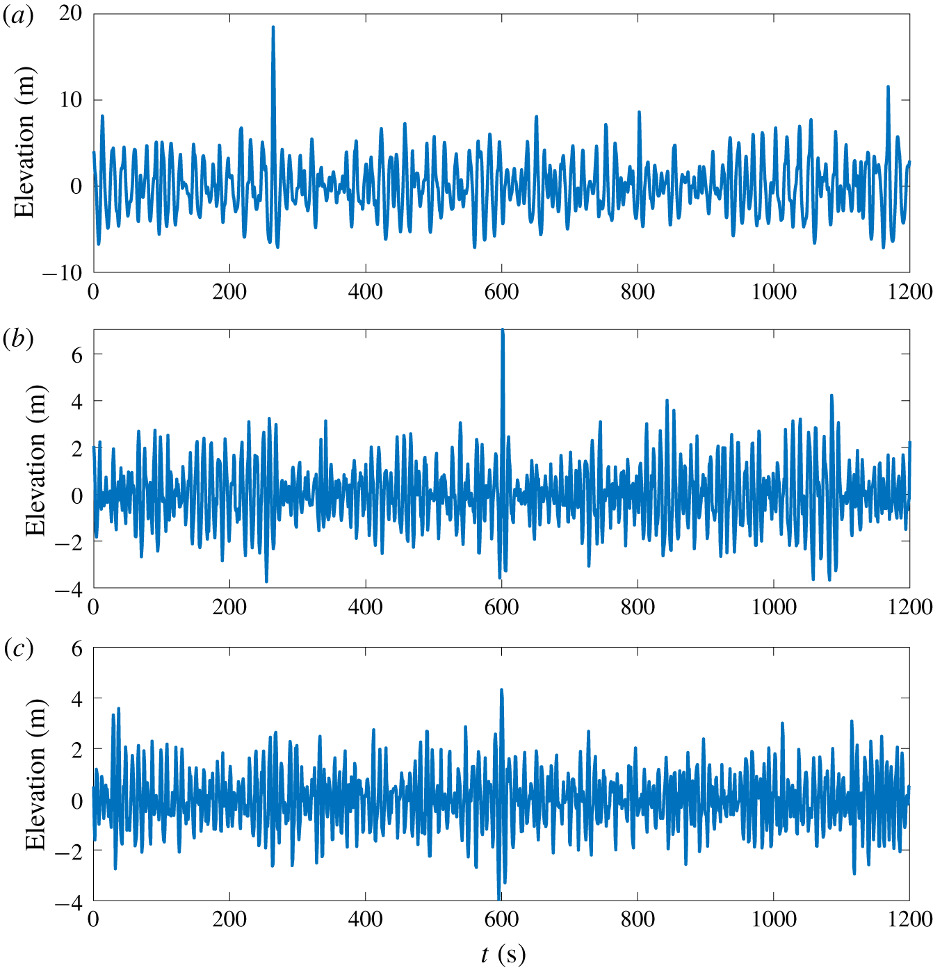
For this study, the reproduction of three different rogue wave profiles is investigated. The first one is the well-known New Year wave recorded on 1 January 1995 at the Draupner platform in the North Sea (Haver Reference Haver2004). This was the first scientific measurement of a rogue wave, and as such has been widely studied as a reference event for extreme waves. This famed wave has been accurately reconstructed using the interference or dispersive focusing mechanism in a unidirectional wave flume (Clauss & Klein Reference Clauss and Klein2011) and more recently in a directional flume for crossing seas with a crossing angle of  $120^{\circ }$ (McAllister et al. Reference McAllister, Draycott, Adcock, Taylor and Van Den Bremer2019). The second and third wave profiles have been measured in the Sea of Japan at a location 3 km off the Yura fishery harbour (Mori, Liu & Yasuda Reference Mori, Liu and Yasuda2002). The temporal free-surface profiles for the three rogue waves chosen are given in figure 1 over a standard time window of 20 min.
Full-scale measured wave profiles. (a) New Year wave. (b) Yura wave 1. (c) Yura wave 2.

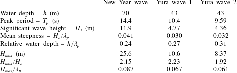
Table 1 summarizes the characteristic properties of the three different rogue wave profiles chosen in this study. The degree of nonlinearity is characterized by the ratios  $H_{max}/H_{s}$ and
 $H_{max}/\unicode[STIX]{x1D706}_{p}$. Here
 $H_{max}$ stands for the maximum wave height extracted from the temporal signal with zero up-and-down-crossing analyses,
 $H_{s}$ is the significant wave height defined from the wave spectrum
 $S(f)$ as
 $H_{s}=H_{m_{0}}=4\sqrt{m_{0}}=4\sqrt{\int S(f)\,\text{d}f}$ and
 $\unicode[STIX]{x1D706}_{p}$ is the peak wavelength defined from the peak period
 $T_{p}$ of the spectrum and the linear dispersion relation
 $\unicode[STIX]{x1D714}=\sqrt{gk\tanh (kh)}$ with
 $h$ standing for the water depth. Ratio
 $H_{max}/H_{s}$ describes the so-called abnormality index (Kharif et al. Reference Kharif, Pelinovsky and Slunyaev2009) of the highest wave while
 $H_{max}/\unicode[STIX]{x1D706}_{p}$ is therefore also a measure of the degree of local nonlinearity of the extreme wave event, which should exceed twice the value of the characteristic wave steepness.
Characteristics of the three extreme wave recordings.

Based on these features, the Yura waves are expected to exhibit a lower level of nonlinearity compared to the New Year wave. However, the wave referred to as Yura 1 is expected to have a lower probability of occurrence than the New Year wave, since it manifests a larger abnormality index. Those three waves are relatively steep and it is possible that wave breaking may have occurred for the extreme waves detected, even if the mean steepness of the wave fields  $H_{s}/\unicode[STIX]{x1D706}_{p}\in [0.030;0.040]$ is not among the steepest possible sea states (see e.g. measurements in the North Sea (Haver, Eik & Meling Reference Haver, Eik and Meling2002; Ducrozet, Bonnefoy & Perignon Reference Ducrozet, Bonnefoy and Perignon2017)). All three events appear in intermediate water depth, characterized by the relative water depth
 $h/\unicode[STIX]{x1D706}_{p}$.
Those three wave profiles, which have been identified as rogue wave events, show different physical features that will enable the testing of the TR procedure in different contexts. Note that the so-called Yura 2 wave is referenced as a rogue wave, even if the ratio  $H_{max}/H_{s}$ is less than the typical threshold of 2. As detailed in Liu & Mori (Reference Liu and Mori2001), the identification of such extreme events can be achieved using the wavelet spectrum. In the case of rogue waves, strong energy density in the spectrum instantly appears and is carried over to the high-frequency components, even at an early stage of evolution (Cousins & Sapsis Reference Cousins and Sapsis2016).
2.3 Experimental study in a water-wave tank
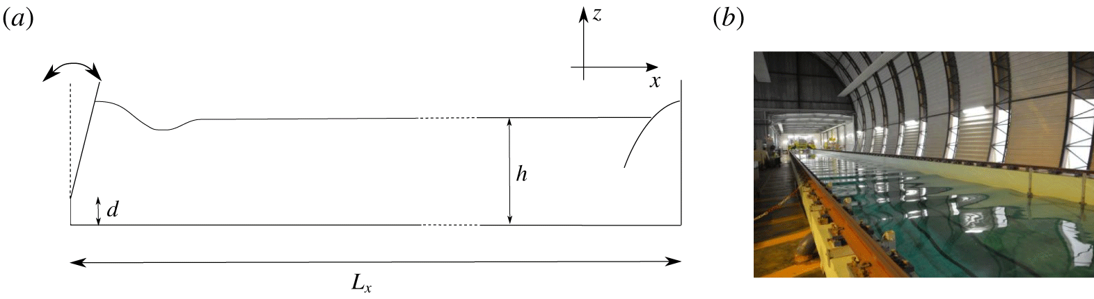
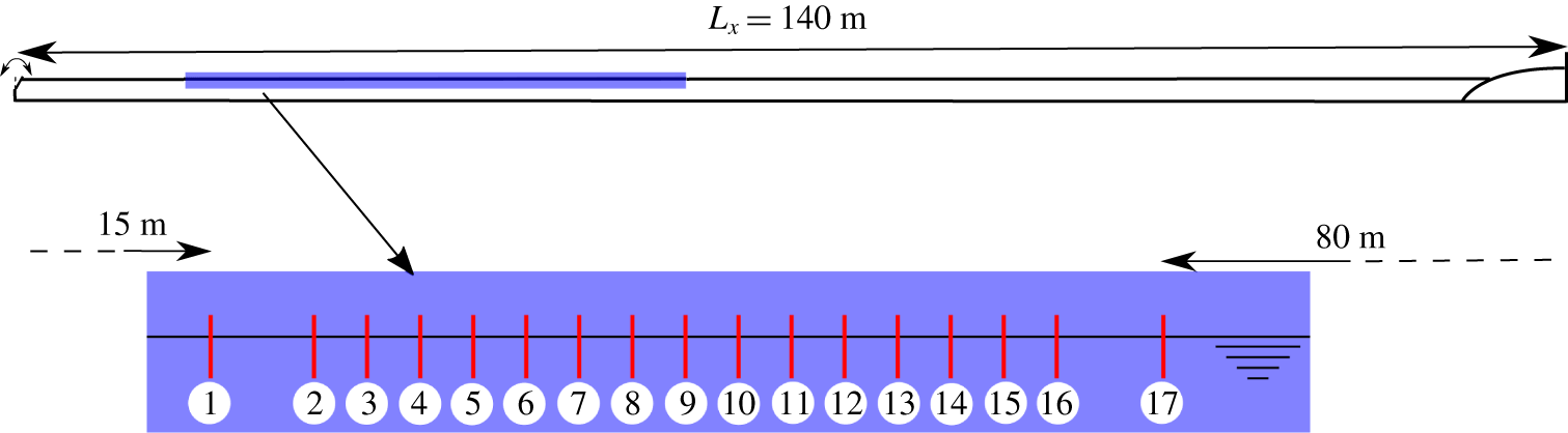
The present set of experiments is conducted in the large-scale towing tank of ECN, which is  $L_{x}=140$ m long, 5 m wide and
 $h=3$ m deep. Figure 2 provides a schematic view of the facility along with a photo. It is equipped with a flap-type wavemaker on one side of the tank to generate a unidirectional wave field in the range
 $f\in [0.15;2]$ Hz. This wavemaker is hinged at a distance
 $d=0.15$ m from the bottom while its displacement can be accurately controlled. On the other side of the tank, an absorbing beach is installed to limit the wave reflections. The main advantage of the present wave tank is its length, which allows measurements free of any reflected waves considering a significant time window (equation (2.2)).
(a) Sketch of the towing tank. (b) Photo of the installation.

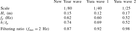
Characteristics of the sea states at model scale.

2.3.1 Choice of wave scales
When performing experiments in a wave tank, the corresponding scale has to be chosen carefully regarding the Froude similarity in use in the present case of gravity waves. In addition, the possible limitations of the generation system, which include the maximum displacement of the paddle, its maximum velocity as well as the frequency range, have to be taken into account for an accurate wave generation. The latter constraints are particularly important when dealing with highly nonlinear waves exhibiting broad frequency content. The wave generator in the towing tank facility can accurately generate waves from frequency  $f_{min}=0.15$ Hz up to
 $f_{max}=2$ Hz. Regarding the latter limit, it is necessary to filter out the higher frequencies, which will not be generated correctly. This may induce significant discrepancies in the expected free-surface elevation if the scale is not chosen correctly, i.e. if the scale is not adapted to the facility with significant energy content above
 $f_{max}$.
As a complement, the geometry of the experimental facility has to be considered. It is indeed necessary to scale the water depth in order to have the exact same physics for wave evolution between real and model scale. However, the flap-type wavemaker prevents the changing of the water depth in our experiments since a reduction induces a decrease of the largest wave possibly generated. Then, the wave field has to be scaled using the previously described wavemaker capabilities, favouring the accuracy of the waves generated over the scaling of the water depth. The TR procedure is applied here to reproduce a temporal wave signal in a tank of arbitrary water depth.
As a consequence, the choice of the scale for the three locally focused reference wave profiles chosen is different as reported in table 2. In this table the significant wave height, the peak frequency  $f_{p}$ and the relative water depth at model scale together with a so-called filtering ratio are presented. Comparing with table 1, the model-scale configuration appears to be in a deep-water regime for the three reference extreme waves. This implies that the underlying physics of the full-scale and model-scale wave fields are different. Indeed, the change in relative water depth is expected to enhance the effect of modulational instability in the proposed experiments compared with the measurements at sea. However, it is anticipated that the assessment of the quality of the TR reproduction procedure in a tank of arbitrary water depth applies to a configuration in which correct Froude scaling is used.
The filtering ratio corresponds to the effect of the wavemaker’s limited-accuracy frequency range on the amplitude of the extreme wave generated. The original ocean rogue wave measurements at sea, as shown in figure 1, are filtered with a low-pass filter in the range  $[0;f_{max}]$. Then, the filtering ratio compares the amplitude of the filtered extreme wave with the amplitude of the original measurement.
2.3.2 Experimental set-up
A set of 17 wave gauges is installed along the wave tank in order to record the temporal evolution of the free-surface elevation at different locations in the range  $x\in [15~\text{m};60~\text{m}]$. The exact locations are provided in table 3. A sketch of the configuration with the locations of the probes is shown in figure 3.
Sketch of the towing tank with the location of the probes.

We use resistance-type wave probes, which were calibrated before the experimental campaign. These provide accurate free-surface measurements at a sampling rate of 100 Hz. The data acquisition is triggered by the wavemaker’s motion start in order to ensure a correct synchronization of the measurements.
Probe locations in the wave tank.

2.3.3 Set of experiments
As reported in Ducrozet et al. (Reference Ducrozet, Fink and Chabchoub2016b), the TR method in deep water is influenced by the steepness of the wave field as well as the distance from the wave generator chosen for the mirror location  $x_{M}$. This governed the choice of the set of tests presented in the next section. In view of covering the reproduction of a large range of wave profile features, both the amplitude of those waves and the mirror location are varied. As a summary, the following tests have been conducted:
(i) The three wave profiles described previously (§ 2.2) are considered, namely New Year, Yura 1 and Yura 2 waves.
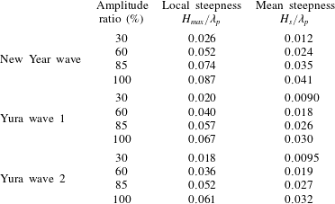
(ii) Different amplitude ratios are tested for each rogue wave profile. This ratio is the scaling applied to the target free-surface elevation, keeping the time scale unchanged, in order to test the influence of the steepness on the quality of the wave reconstruction using TR.
(iii) Three different probes are used as mirror locations
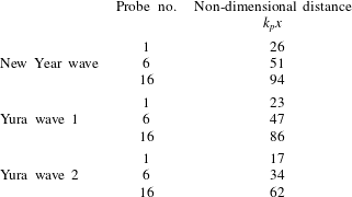
 $x_{M}$. These define the distance of the wave reconstruction from the wavemaker. These probes are referred to by numbers 1, 6 and 16 in table 3. The corresponding distances are $x_{M}\in [15~\text{m};30~\text{m};55~\text{m}]$.


Tables 4 and 5 summarize the corresponding characteristics of the wave field in terms of local and mean steepness as well as the relative propagating distances at the three locations chosen.
Local and mean steepnesses as a function of the amplitude ratio for the three different wave profiles.

Relative propagating distances as a function of the probe used for TR for the three wave profiles.

3 Experimental results
In this section we report the experimental analysis related to the reconstructed ocean extreme sea states as in the North Sea and Sea of Japan using the TR approach. We first discuss the observations relative to the presence of breaking waves during the experiments. Then, we report an example of wave profiles, obtained during the first propagation, before presenting the comprehensive results of the reconstruction procedure.
3.1 Experimental step 1: reference extreme wave generation
The presence of breaking waves in the course of the experiments is crucial in the context of the TR method. This procedure indeed relies on the reversibility of the wave propagation process. This reversibility condition can be violated when wave breaking occurs. This phenomenon is known to induce wave energy dissipation through viscosity, mixing, etc., which are non-reversible effects (Babanin Reference Babanin2011).
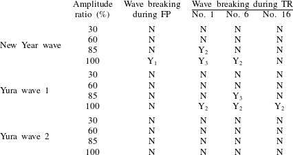
It is then expected that the presence of wave breaking has a strong influence on the quality of the TR reconstruction. Table 6 provides a summary of the observations during the experiments with respect to the presence of wave breaking.
Observations during experiments: first propagation (FP) and TR. Here Y and N stand for yes and no with respect to the presence of wave breaking in the course of the experiment. Subscript 1 indicates a wave breaking close to the wave generation system, 2 indicates a wave breaking close to the wave probe and 3 denotes a wave breaking just after the wave probe.

During the first propagation, it is expected that a rogue wave, which is highly localized in space and time, will defocus and disperse during its propagation when generated by the wave generator at  $x_{S}$. The wave breaking probability is consequently expected to be larger close to the wavemaker. It was observed that the New Year wave at maximum amplitude is the only configuration experiencing wave breaking, which indeed appears localized close to the wavemaker.
As a complement, during the effective reproduction of the extreme wave profiles, refocusing will occur up to the mirror location  $x_{M}$ chosen for the TR approach. Wave breaking, if present, is expected to be located close to this probe during the TR reconstruction process. In the experiments conducted, both New Year and Yura 1 waves are prone to the appearance of breaking waves, due to the significance of the local steepness of these waves (see table 1). These events always appear at the focusing region and are limited, as expected, to the highest amplitude ratios of 85 % and 100 %.
3.2 Wave propagation tracking and wave reflection analysis
During the first propagation of the wave field, the results are similar in terms of wave reflection analysis for the three wave profiles being considered. We consequently limit the content of this section to the case of the New Year wave.
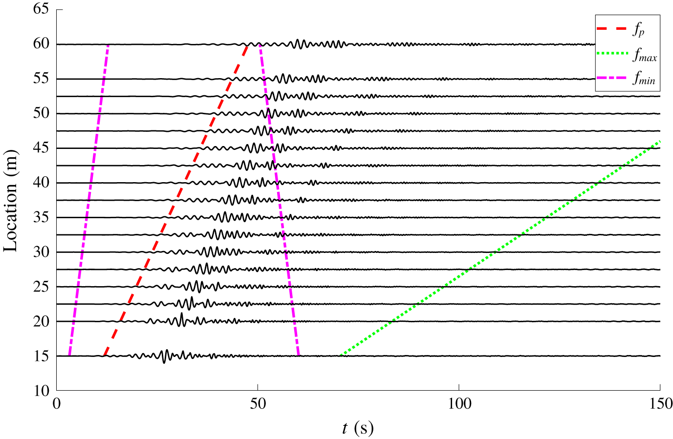
Figure 4 presents the temporal free-surface profiles for the 17 wave gauges obtained for the 100 % amplitude-scaled New Year wave (i.e. the target rogue wave). For clarity, the different probes are vertically shifted with respect to their location in the water tank. In addition, figure 4 includes different lines that depict the location of the wave fronts at the different probe locations. Those are useful for assessing the possible presence of wave reflection during the measurements. Here, three different wave fronts are considered:
(i) Line
$f_{min}$ depicts the propagation of the wave front associated with the lower-frequency waves generated by the wavemaker. This indicates the location of this wave front for each temporal probe signal. The second part of the line (vertically descending) represents this wave front after its reflection on the absorbing beach. This line is essential to analyse the presence of wave reflections in the experiments conducted.(ii) Line
$f_{p}$ is the same as the previous one, but for the peak frequency.(iii) Line
$f_{max}$ represents the location of the wave front associated with the maximum frequency $f_{max}$ generated by the wavemaker. It starts at the end of the first propagation time window $T_{win_{FP}}$ to depict the wave front of the end of the experiment (also referred to as wave tail). This is the final time with relevant frequency content, which consequently defines the time window in use for the TR experiment (2.1).


First propagation for New Year wave with 100 % amplitude. Vertically shifted probe temporal signals (solid lines) together with wave fronts for different frequencies (see text for details).

The different probe temporal signals allow an overview of the space–time evolution of the considered wave sequence imposed at the wavemaker location. We can clearly observe the attenuation of the initial rogue wave profile and especially the effect of the dispersion on the initial extreme event. On this relatively long propagation distance  $k_{p}x_{max}\simeq 100$, we notice that the initial localized free-surface profiles evolve towards different wave packets that propagate with their own speeds.
While observing the different wave fronts, it is also interesting to indicate that it appears almost impossible to eliminate the reflection of the lower frequencies, even if their energy is assumed to be very small over the whole time window used for the refocusing experiment (see dotted green line  $f_{max}$).
On the other hand, if one considers the peak frequency as the relevant one, this ensures a quite large time window free of reflections. From a practical point of view, when considering wave probes further in the wave tank, the amount of reflected waves is assumed to become gradually larger. In this respect, the length of the water tank in use allows one to delay the appearance of those reflected waves and consequently reduce their energy content.
As a reminder, the probes used to determine the mirror location for the TR are probe nos. 1, 6 and 16. They can be consequently considered as free of reflection, with a limited amount of reflection and possibly influenced by reflection, respectively.
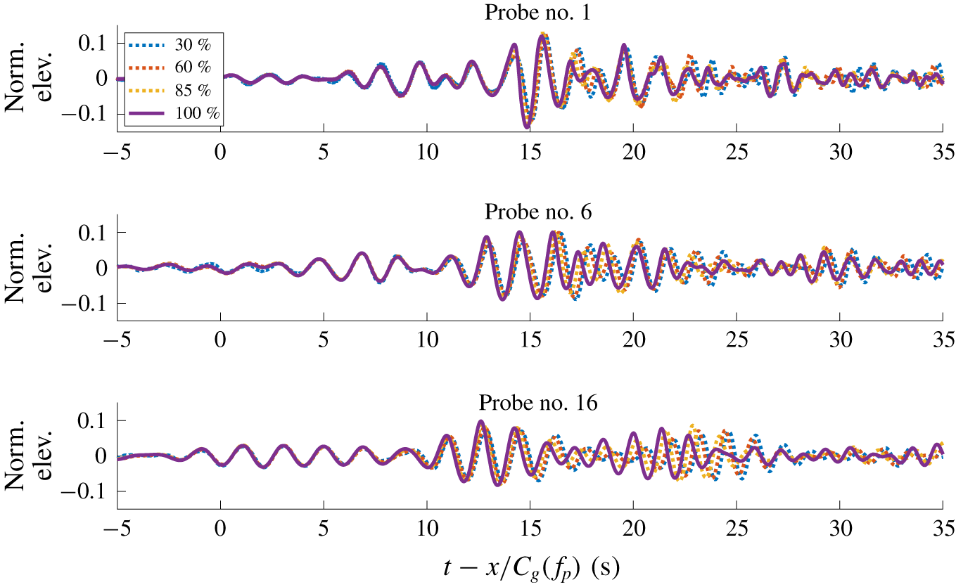
Figure 5 presents the effect of the nonlinearity during the first propagation of the wave field. The normalized free-surface elevation  $\unicode[STIX]{x1D702}^{\ast }=\unicode[STIX]{x1D702}/\text{amplitude ratio}$ is presented at the three probes 1, 6 and 16, which are used in the following for the TR procedure. The time is then shifted with the group velocity at the peak of the wave spectrum
 $C_{g}(f_{p})$ for correct alignment of the wave groups.
Effect of the nonlinearity during first propagation for the New Year wave.

The importance of the nonlinearities during the propagation in the wave tank is clearly demonstrated. Large discrepancies are observed when changing the amplitude ratio of the initial wavemaker motion, especially in terms of phase velocities of the different wave components. In fact, a significant phase shift is observed for probe no. 16. In addition, the crest–trough asymmetry appears also slightly enhanced when increasing the amplitude ratio, even after the demodulation of the extreme wave.
All nonlinear effects are consequently considered in the TR procedure (including, for example, the second- and third-order ones at play in the previous physical features). This is of primary importance for the accuracy of the reconstruction procedure.
3.3 Experimental step 2: refocusing of extreme waves using TR
The TR procedure is applied to the recorded temporal free-surface profile, obtained from the mirror position that corresponds to the wave gauge location. This time-reversed signal is then generated by the wavemaker. Note that for each wave profile four different amplitude ratios are tested first to describe the effect of nonlinearities while three different probes are used to evaluate the effects of dispersion. We refer to table 6 for the observations during the different experiments.
To assess the accuracy of the reproduction, two estimators are introduced. These are the error on the crest amplitude  $\unicode[STIX]{x1D716}_{c}$ and the global error on the free-surface elevation
 $\unicode[STIX]{x1D716}_{\unicode[STIX]{x1D702}}$ corresponding to the normalized mean square error of the reproduction procedure. They are defined as
 $$\begin{eqnarray}\displaystyle & \displaystyle \unicode[STIX]{x1D716}_{c}=1-\frac{\displaystyle \max _{t}(\unicode[STIX]{x1D702}_{TR}(t))}{\displaystyle \max _{t}(\unicode[STIX]{x1D702}_{t}(t))}, & \displaystyle\end{eqnarray}$$
 $$\begin{eqnarray}\displaystyle & \displaystyle \unicode[STIX]{x1D716}_{\unicode[STIX]{x1D702}}=\frac{\displaystyle \int _{0}^{T_{win}}|\unicode[STIX]{x1D702}_{TR}(t)-\unicode[STIX]{x1D702}_{t}(t)|^{2}\,\text{d}t}{\displaystyle \int _{0}^{T_{win}}|\unicode[STIX]{x1D702}_{t}(t)|^{2}\,\text{d}t}, & \displaystyle\end{eqnarray}$$
with  $\unicode[STIX]{x1D702}_{t}(t)$ being the temporal target free-surface profile (i.e. the signal recorded at sea) and
 $\unicode[STIX]{x1D702}_{TR}(t)$ the temporal free-surface profile obtained after TR. Note that values close to zero for both errors correspond to an efficient reproduction procedure.
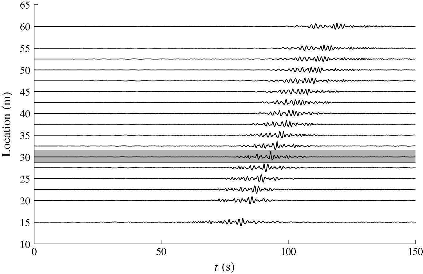
Refocusing of the extreme event on probe no. 6 (identified in grey). New Year wave, 100 % amplitude. Probe signals are vertically shifted with respect to their location in the wave tank.

3.3.1 New Year wave
An example of wave refocusing is presented in figure 6, making use of the whole set of available wave gauges, in order to observe the unidirectional space–time evolution in the wave tank. The different probe records are vertically shifted with respect to their location in the water tank.
The reproduction location of the extreme wave is probe no. 6, which is identified in the grey zone in the plot. The refocusing process is indeed clearly observed and confirmed, followed by the demodulation of the extreme event created exactly at the target location  $x_{M}$.
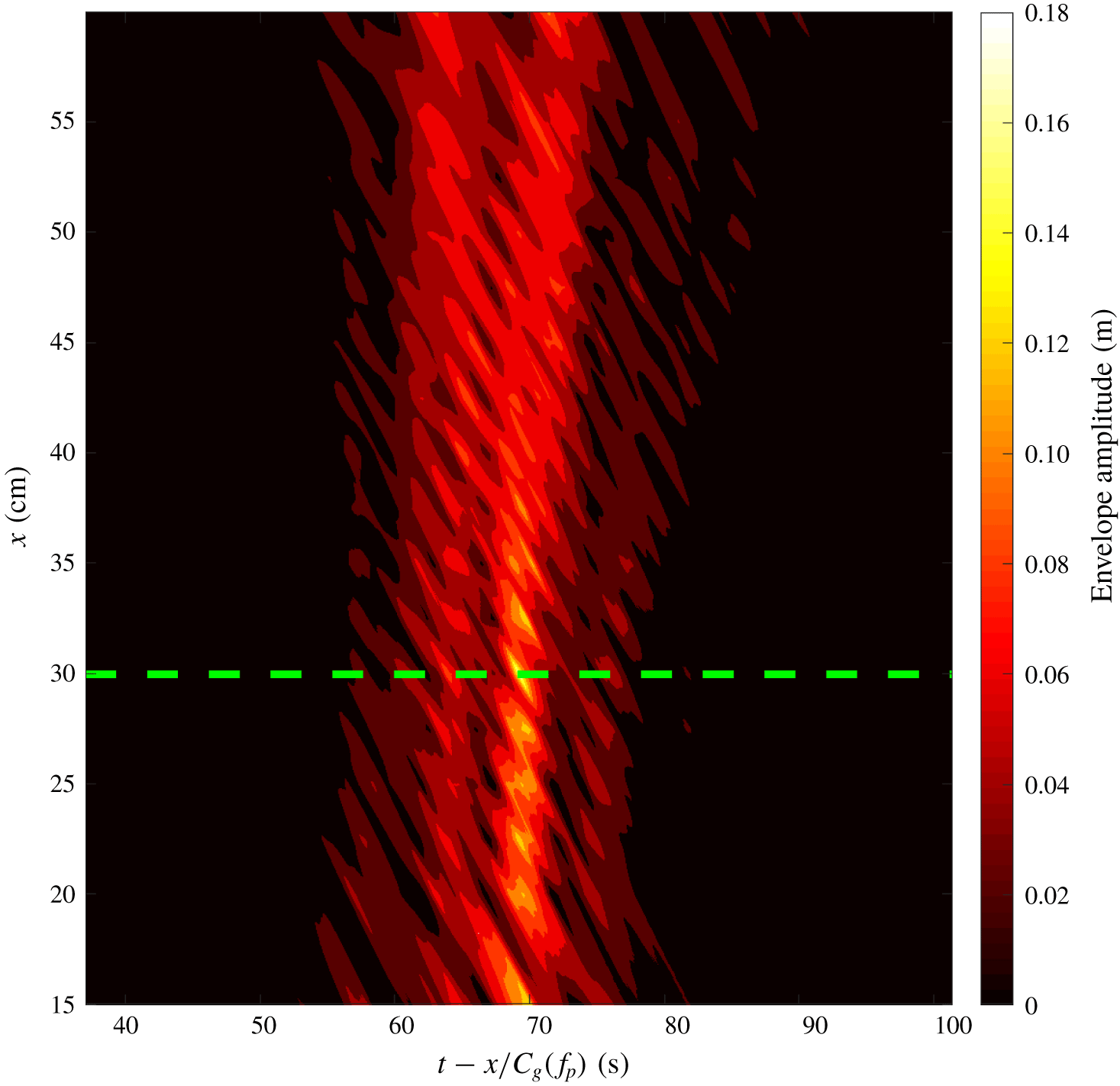
Figure 7 presents the space–time evolution of the envelope of the signal, which is a typical representation in the context of the NLSE. The time has been adjusted by the value of the group velocity at the peak of the spectrum  $C_{g}(f_{p})$ in order to align the propagation of wave packets only.
Refocusing of the extreme event, space–time representation. New Year wave, 100 % amplitude, refocusing on probe no. 6 (identified with the green dashed line).

The focusing/defocusing process is also quite clear with a change in the amplitude of the envelope together with an increase of its spatial spreading after the reproduction of the rogue event in the wave flume.
In order to quantify the analysis, the reproduced wave profiles need to be compared with the target wave signal and an evaluation made of the error estimators previously introduced. These are  $\unicode[STIX]{x1D716}_{c}$ and
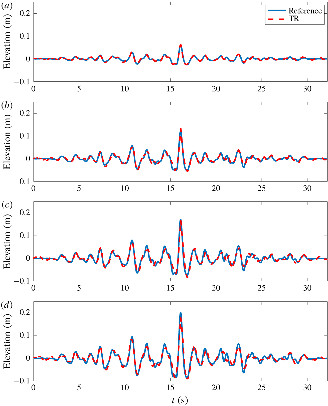
 $\unicode[STIX]{x1D716}_{\unicode[STIX]{x1D702}}$. As an example of results, figure 8 depicts a comparison of the temporal free-surface profiles of the reproduction of the New Year wave on probe no. 1 for the different amplitude ratios of 30, 60, 85 and 100 %.
Comparison of the original wave profile and the TR reconstructions at probe no. 1,  $x_{M}=15$ m. New Year wave with different amplitude ratios of 30, 60, 85 and 100 % from (a) to (d).

The effect of nonlinearity in the TR reconstruction process appears to be obvious. While with an amplitude ratio of 30 % the wave profile is perfectly reproduced over the whole time window, discrepancies are more important with an increase of the amplitude and, thus, nonlinearity. This confirms previous study results reported in Ducrozet et al. (Reference Ducrozet, Fink and Chabchoub2016b). However, the error remains remarkably limited in the present configuration for all amplitudes.
As indicated in table 6, the first propagation at 100 % amplitude is subjected to a local wave breaking close to the wavemaker. It is striking that even in the presence of this irreversible process, the TR procedure is accurate in reproducing the initial wave profile ( $\unicode[STIX]{x1D716}_{\unicode[STIX]{x1D702}}=0.09$), with a minor loss of the amplitude of the crest (
 $\unicode[STIX]{x1D716}_{c}=0.10$). The breaking process probably removes a limited amount of energy, allowing an accurate reproduction of the target wave profile.
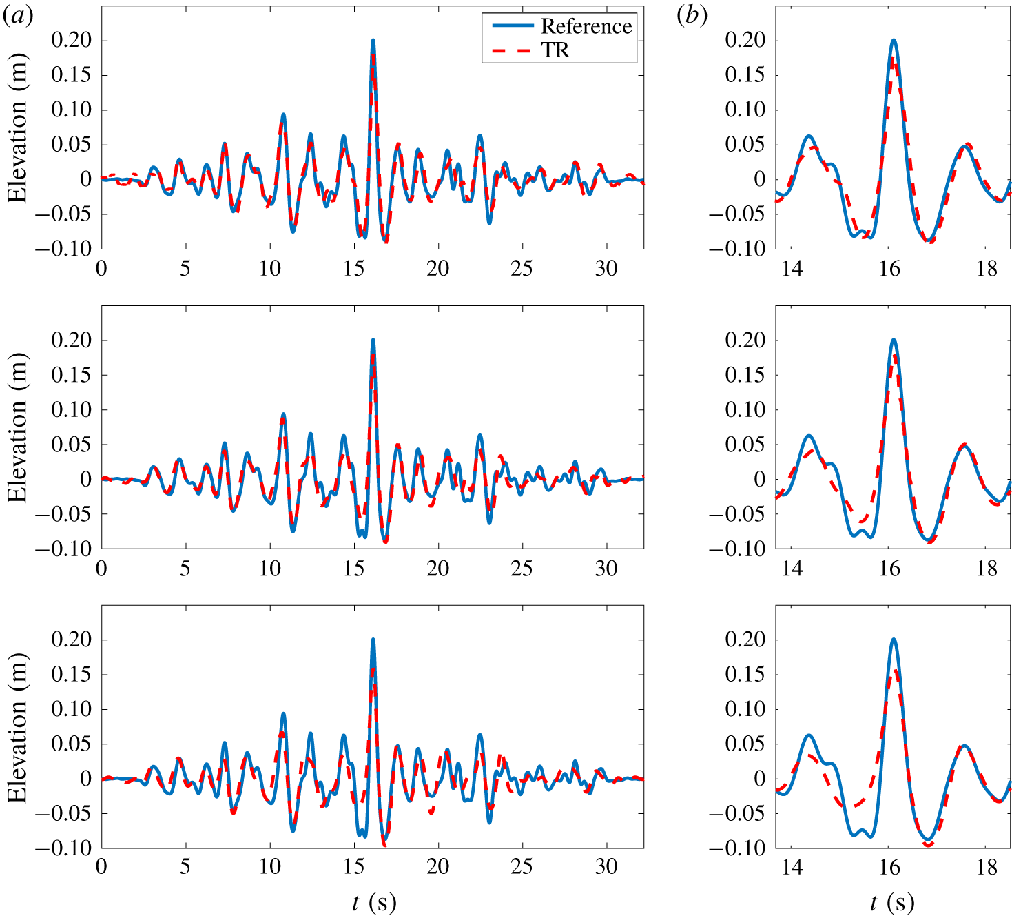
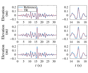
In order to characterize the dispersive effects over the propagating distance, figure 9 depicts the reproduced free-surface profiles at the three different locations corresponding to probe nos. 1, 6 and 16 for the case of the New Year wave at 100 % amplitude scale. As a reminder, the corresponding propagating distances are  $[4\unicode[STIX]{x1D706}_{p};~8\unicode[STIX]{x1D706}_{p};~15\unicode[STIX]{x1D706}_{p}]$, respectively.
Comparison between original wave temporal profile and after TR for New Year wave at 100 % amplitude scale. Different mirror locations, probe nos. 1, 6 and 16 from top to bottom. Complete reconstructed wave profile (a) and zoom on the extreme event (b).

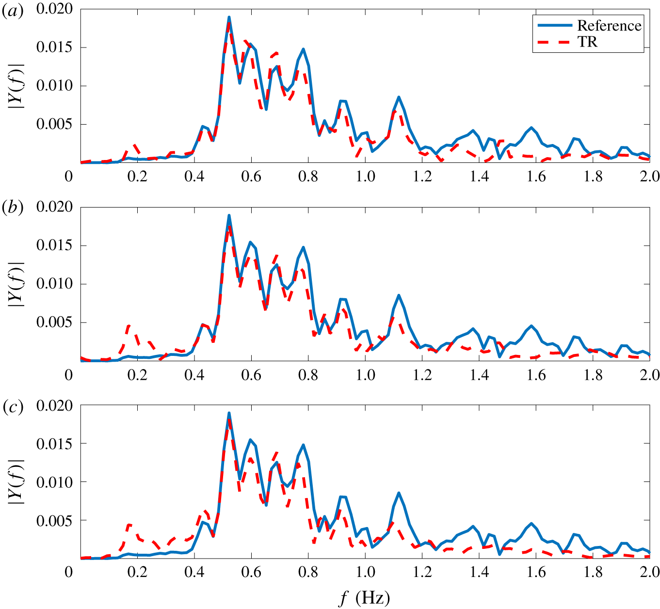
In addition to the temporal free-surface profiles, figure 10 shows the magnitude of the Fourier components of the signal  $Y(f)$. This allows a more accurate characterization of the differences between the target signal and the reproduced one.
Comparison between Fourier transform modulus of the original wave profile and after TR for New Year wave at 100 % amplitude scale. Different mirror locations, probe nos. 1, 6 and 16 from (a) to (c).

It is evident that the TR procedure is highly influenced by the propagating distance, and, thus, dispersive effects, which degrade the quality of the reproduction. Comparisons in the time and frequency domains demonstrate significant differences between the target and reproduced signals, especially at the location of probe no. 16. As noted in § 3.2, this last probe is expected to be influenced by the waves reflected from the absorbing beach. This observation holds true for the first propagation as well as for the refocusing experiment.
An analysis of the frequency domain comparison indicates that the discrepancies between target and reproduced signals become increasingly important in the lower part of the spectrum when increasing the propagating distance. This is indeed a direct consequence of the wave reflection that concerns primarily the fastest wave components.
Some discrepancies are also observed in the high-frequency range of the spectrum  $f>f_{p}$, which may be attributed to the residual inaccuracies in the wave generation, even with the second-order corrections provided in the present study. Those may be enhanced during the propagation process due to the different nonlinear interactions between components.
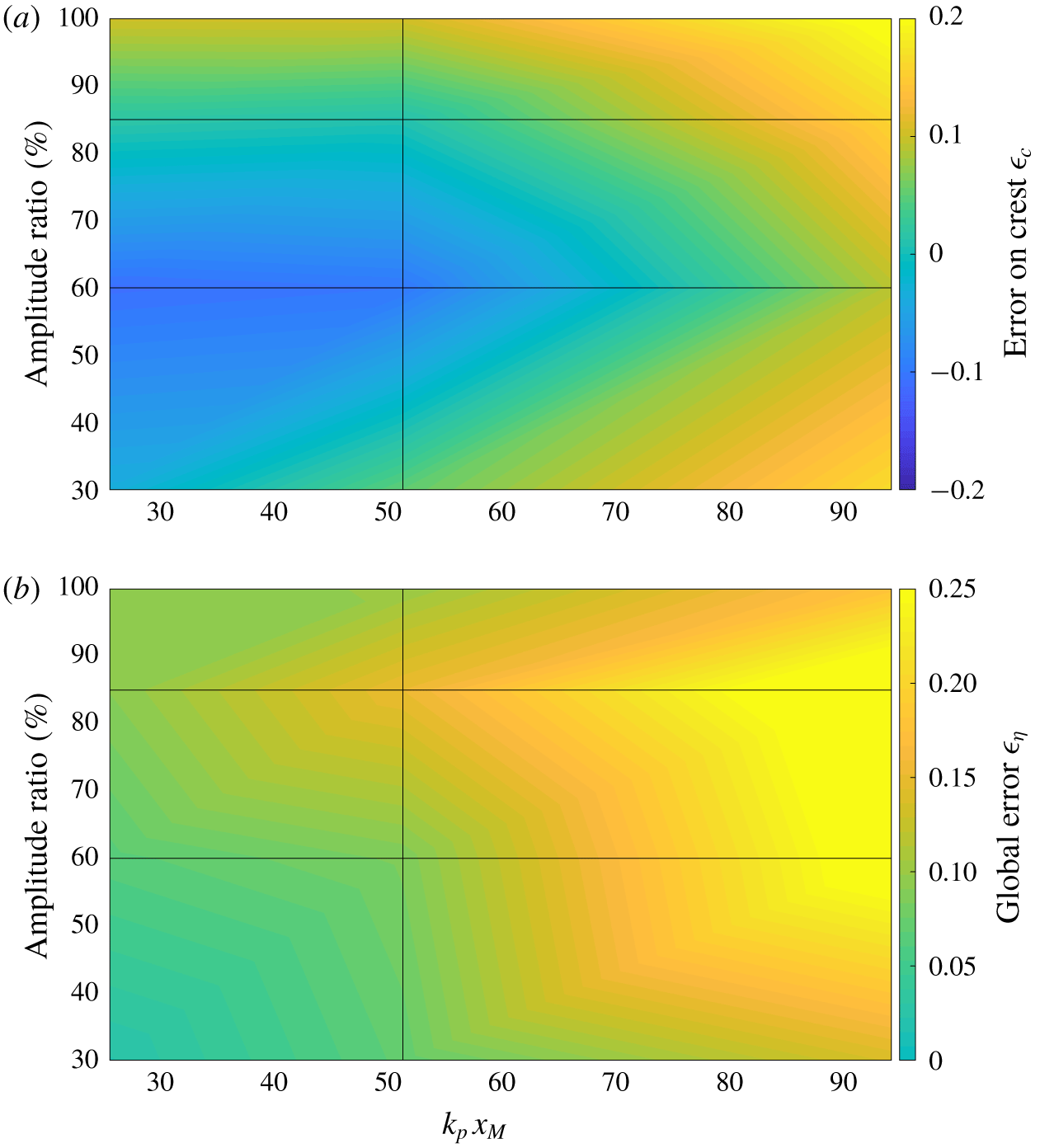
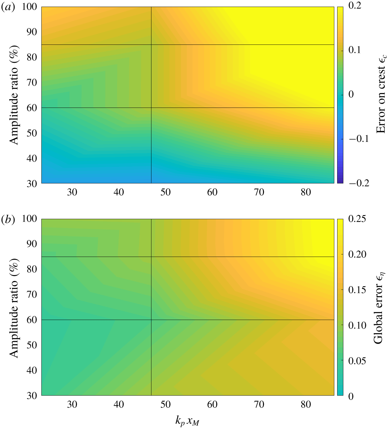
In order to quantify these observations, figure 11 gives the errors on the amplitude of the crest as well as that on the whole temporal profile for the New Year wave. It allows an analysis of the accuracy of the method of reproduction, similarly to the numerical work of Ducrozet et al. (Reference Ducrozet, Fink and Chabchoub2016b). The location of the mirror and the amplitude ratio are varied, to assess the effects of dispersion and nonlinearity, respectively.
Quality of TR reconstruction for the New Year wave as a function of mirror location and amplitude ratio. (a) Error on crest amplitude  $\unicode[STIX]{x1D716}_{c}$. (b) Global error on free-surface elevation
 $\unicode[STIX]{x1D716}_{\unicode[STIX]{x1D702}}$.

We recover the influences previously described, namely that an increased propagating distance reduces the accuracy of the reproduction. At the same time, an increased nonlinearity also affects the TR procedure, however in a more limited way. The levels of accuracy are indeed satisfying in the range  $k_{p}x_{M}\leqslant 50$.
The TR procedure, which is a straightforward process to set up experimentally compared to existing ones based on dispersive focusing, such as the New Wave theory (Tromans et al. Reference Tromans, Anaturk and Hagemeijer1991; Chaplin Reference Chaplin1996; Clauss & Schmittner Reference Clauss and Schmittner2007; Schmittner et al. Reference Schmittner, Kosleck and Hennig2009; Fernandez et al. Reference Fernandez, Sriram, Schimmels and Oumeraci2014; Ducrozet et al. Reference Ducrozet, Bonnefoy and Ferrant2016a), consequently manages to accurately reproduce highly nonlinear extreme events such as the New Year wave in a straightforward way. The presence of wave breaking during the first experiment or during the refocusing did not lead to a failure of the complete procedure, demonstrating its robustness.
3.3.2 Yura 1 wave
Figure 12 presents an overview of the errors after reproduction with a varying level of nonlinearity and propagating distance in the case of the Yura 1 wave field. As a reminder, this rogue wave, compared to the previously discussed New Year wave, appeared in a wave field with lower steepness, but exhibited a larger abnormality index  $H_{max}/H_{s}$ that corresponds to a lower probability of occurrence (see table 1).
Quality of TR reconstruction for the Yura 1 wave as a function of mirror location and amplitude ratio. (a) Error on crest amplitude  $\unicode[STIX]{x1D716}_{c}$. (b) Global error on free-surface elevation
 $\unicode[STIX]{x1D716}_{\unicode[STIX]{x1D702}}$.

The results for the Yura 1 wave appear similar to those obtained for the New Year wave. Indeed, an increased steepness of the wave profile to reproduce an increased relative propagating distance induces a reduction of the accuracy of the reproduction, in terms of both the maximum amplitude of the reproduced wave  $\unicode[STIX]{x1D716}_{c}$ and global error
 $\unicode[STIX]{x1D716}_{\unicode[STIX]{x1D702}}$.
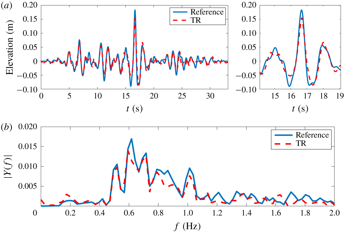
We also observe that the free-surface profile of the 100 % amplitude on probe no. 1 appears less accurate for this wave profile. As a matter of completeness for figures 9 and 10, figure 13 presents a comparison of the target and reproduced wave profiles for this specific configuration.
Comparison between original wave profile and after TR construction for Yura 1 wave at 100 % amplitude scale at probe no. 1. Time domain (a) and frequency domain (b).

As noted in table 6, wave breaking has been observed during the refocusing experiment for this specific configuration. It takes place at the exact location of the probe, as a result of the high degree of nonlinearity of this wave. For the New Year wave, it was clear that the breaking occurs after the target wave probe when using probe no. 1. This is different for the present configuration in which the breaking appears close and just prior to the probe and is consequently expected to dissipate a part of the wave energy. This induces different behaviours in both configurations and especially for the Yura 1 wave a less accurate reconstruction on probe no. 1, which exhibits an error of  $\unicode[STIX]{x1D716}_{c}=0.15$ and
 $\unicode[STIX]{x1D716}_{\unicode[STIX]{x1D702}}=0.10$.
Nevertheless, the levels of errors are notably good for the Yura 1 wave profile over the whole range of amplitudes up to the most extreme measured one and for limited propagating distances  $k_{p}x_{M}\leqslant 50$.
3.3.3 Yura 2 wave
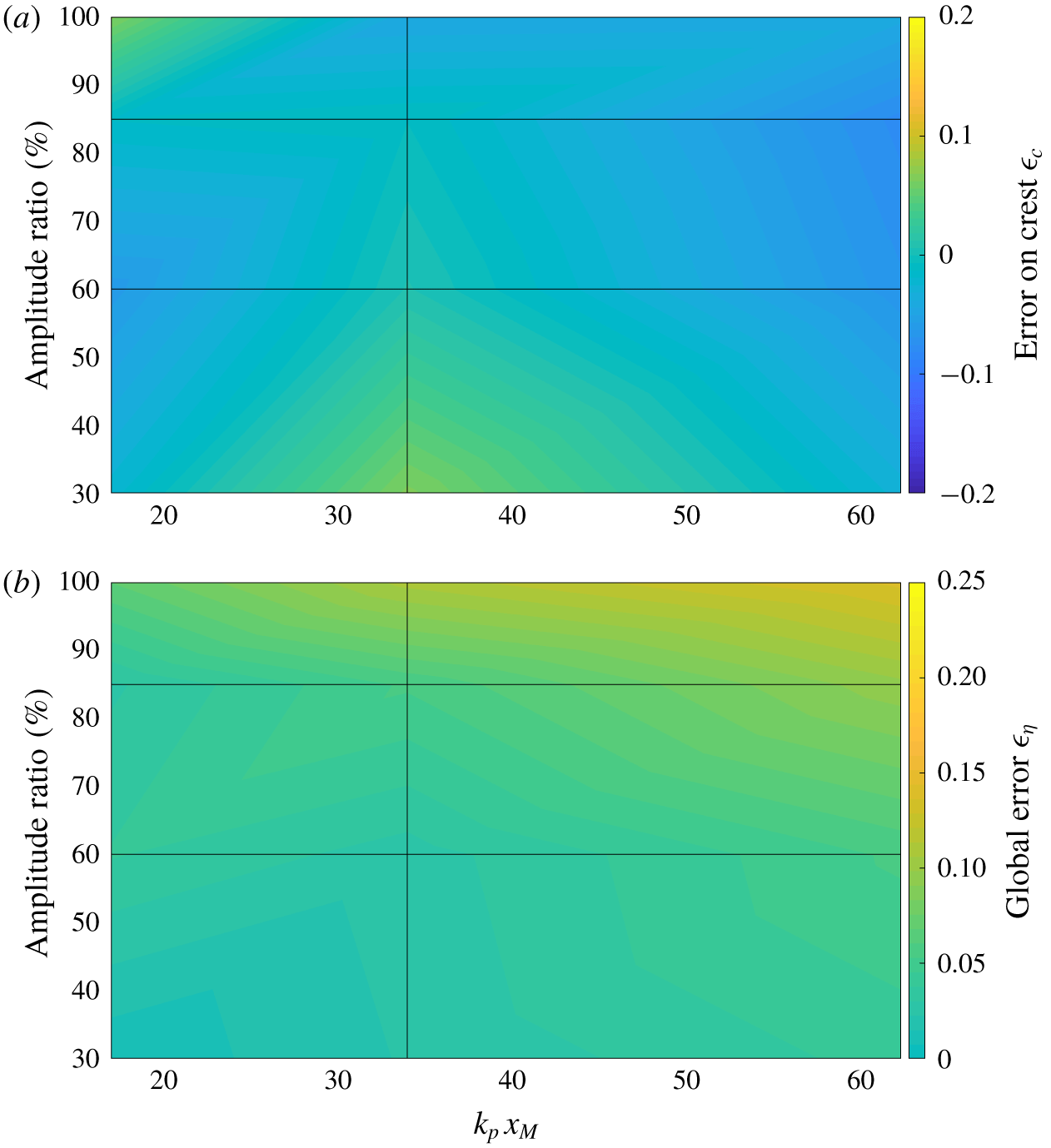
The Yura 2 wave has the lowest abnormality index value among the three tested (see main characteristics in table 1). Figure 14 shows the overview of the errors after reproduction with a varying level of nonlinearity and dispersive length.
Quality of TR reconstruction for the Yura 2 wave as a function of mirror location and amplitude ratio. (a) Error on crest amplitude  $\unicode[STIX]{x1D716}_{c}$. (b) Global error on free-surface elevation
 $\unicode[STIX]{x1D716}_{\unicode[STIX]{x1D702}}$.

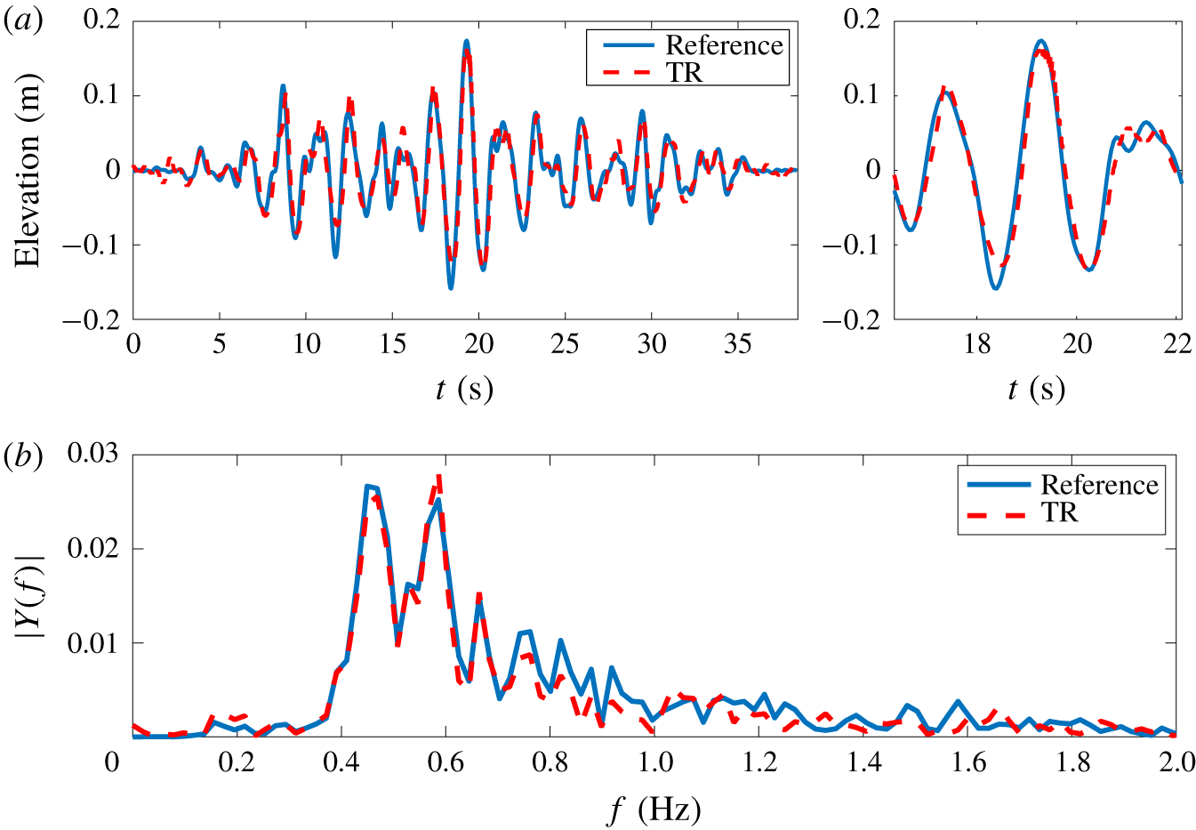
The observations are similar to the previous ones. These are mainly that an increase of the propagating distance and degree of nonlinearity reduces the accuracy of the reconstruction using the TR procedure. However, when comparing the results to the features of the New Year and Yura 1 waves as depicted in figures 11 and 12, we note that the errors are far smaller for the Yura 2 wave profile. This is a direct consequence of the reduced degree of nonlinearity of this wave profile, which is less steep compared to the previously discussed wave configurations. To quantify those differences and as a matter of comparison, figure 15 presents the target and reproduced free-surface profiles for the 100 % amplitude scale at the location of probe no. 1.
Comparison between original wave profile and TR reconstruction for the Yura 2 wave at 100 % amplitude scale at probe no. 1. Time domain (a) and frequency domain (b).

As expected, the reproduction appears very accurate in this configuration. It is characterized by errors  $\unicode[STIX]{x1D716}_{c}=0.06$ and
 $\unicode[STIX]{x1D716}_{\unicode[STIX]{x1D702}}=0.07$. The remaining differences may be attributed to the reflections and other discrepancies that may appear in the course of the TR procedure and during the wave generation.
4 Conclusion
The present work reports a detailed study of the use of the TR methodology for the reproduction of recorded real-world extreme waves in physical unidirectional wave tanks. The objective is to assess the applicability and accuracy of the TR reproduction procedure in this new configuration consisting of genuine rogue waves, embedded in their irregular sea state. To this end, a set of experiments has been carried out in the 140 m long towing tank of ECN. Different wave profiles, obtained from real measurements at sea, have been used: (i) the famed New Year wave and (ii) two freak wave events recorded in the Sea of Japan.
The design of model-scale experiments for ocean waves is done using Froude scaling. However, it is applied here in a wave tank of arbitrary water depth, due to experimental constraints. The relative water depth is consequently different in model-scale and full-scale configurations, leading to possible different physical processes during wave propagation. Nevertheless, the different features of the TR method revealed in the current experiments are expected to be relevant when exact Froude scaling is used.
The experiments have been designed to test the influence of the two main parameters presented in Ducrozet et al. (Reference Ducrozet, Fink and Chabchoub2016b), namely the relative propagation distance  $k_{p}x_{M}$ or dispersive length and the effect of the degree of nonlinearity, independently of the generation mechanism at play. These parameters have been varied over a wide range and have been demonstrated to be also of major importance in the present configuration and study.
We confirmed that the experimental two-step TR procedure can indeed be used for the reproduction of realistic ocean extreme waves in a laboratory environment. The main advantage of the methodology is the refocusing generation of extreme waves at almost any arbitrary position in the wave facility independently of the focusing mechanism at play. An increased steepness of the targeted wave profile and an increase of the relative propagating distance influence the accuracy of the reproduction. The levels of errors observed experimentally with a real free-surface measurement of a rogue wave appear similar to those observed experimentally (Chabchoub & Fink Reference Chabchoub and Fink2014) and numerically validated (Ducrozet et al. Reference Ducrozet, Fink and Chabchoub2016b) using analytic solutions of the NLSE, such as the doubly localized Peregrine-type breathers (Chabchoub et al. Reference Chabchoub, Onorato and Akhmediev2016) known to be considered as possible backbone prototype rogue waves (Akhmediev, Ankiewicz & Taki Reference Akhmediev, Ankiewicz and Taki2009; Shrira & Geogjaev Reference Shrira and Geogjaev2010).
The only discrepancies observed are relative to the spatial extent, which is rather limited in the present experiments compared to the numerical computations. The influence of the relative propagating distance appeared to be driven by the presence of wave reflection instead of presenting a possible inherent limitation of the methodology. Further work using a numerical wave tank that includes all physical processes at play, such as HOS-NWT (Ducrozet et al. Reference Ducrozet, Bonnefoy, Le Touzé and Ferrant2012), may be useful in this context as well. This would allow the overcoming of the physical limitations of experimental wave flume configurations in terms of dimensions, presence of wave reflections and limited frequency range. These limitations can be mastered in numerical wave tank experiments.
We demonstrated that the TR method is suitable for accurately reconstructing the free-surface profile of different rogue wave measurements. In the context of wave–structure interactions, the induced kinematics is also of major importance. This is known to be complex and highly influenced by the wave nonlinearities for extreme waves (Yasuda et al. Reference Yasuda, Mori and Nakayama1994; Grue & Jensen Reference Grue and Jensen2006; Alberello et al. Reference Alberello, Chabchoub, Monty, Nelli, Lee, Elsnab and Toffoli2018). However, it is expected that once the free-surface profile is accurately reproduced, the induced kinematics would naturally follow (Ducrozet et al. Reference Ducrozet, Bonnefoy and Ferrant2016a). This particular point will be the subject of further investigations.
In addition to the evidence of its accuracy in the current context, the behaviour of the TR procedure in terms of robustness is outstanding. We demonstrated that the presence of marginal wave breaking during the first propagation or during the refocusing did not lead to a failure of the complete refocusing process. Indeed, general physical limitations when reconstructing rogue waves in the wave flume may be attributed to the presence of wave breaking and the presence of wave reflection.
Despite the slight inaccuracies, the TR principle seems to be the simplest procedure for reconstructing highly nonlinear and steep waves in a wave flume compared to existing procedures (Tromans et al. Reference Tromans, Anaturk and Hagemeijer1991; Chaplin Reference Chaplin1996; Clauss & Schmittner Reference Clauss and Schmittner2007; Schmittner et al. Reference Schmittner, Kosleck and Hennig2009; Fernandez et al. Reference Fernandez, Sriram, Schimmels and Oumeraci2014; Ducrozet et al. Reference Ducrozet, Bonnefoy and Ferrant2016a), since it provides a similar level of accuracy and high robustness, independently of the physical complexities that are at play in the ocean environment.
Acknowledgements
The authors are grateful to Dr S. Haver for providing the experimental data of the New Year wave. Dr S. Bourdier is acknowledged for the help provided during the course of the experiments. This work has been partially supported by MEXT/JSPS KAKENHI in Japan.
Declaration of interests
The authors report no conflict of interest.