During spring 2000, we released to the press a preliminary forecast of a Gore victory. Indeed, one of us, in a widely-read quotation, declared, “It's not even going to be close” (Washington Post, May 26, 2000, p. 1). We were wrong, as were all of our fellow modelers. Indeed, among “five of the best forecasters” identified by Robert Kaiser (Washington Post, May 26, 2000, p. 1), the Gore projection ranged from 53% to 60% of the two-party popular vote, pointing to a Democratic landslide. Such gross error raises the question: Should the models be junked? Some journalists, pundits, and scholars have suggested the answer is “yes.” We disagree. Remember that forecasters of all stripes—modelers, pollsters, marketers, campaign experts—failed to call 2000. (See the review of 49 forecasts, from multiple and international sources, in Lafay and Lewis-Beck 2000). The virtually total inability to predict the Bush-Gore result also reminds us that no model will ever be perfect, that electoral behavior can never be fully determined. Still, while falling short of perfection, we believe that modeling can be improved.
The key to success lies with the reduction of specification error, namely inclusion of the proper independent variables, properly measured. Put another way, better theory will yield better forecasts. As we shall show, models based on sounder theory than that available in 2000 manage to lower prediction error substantially, for the post-World War II election series in general and for the 2000 race in particular. These models inform us more fully about how voters respond, especially with regard to the economy. Here jobs, or their relative lack, play a decisive role that has hitherto been neglected. Once the job market is considered, a rather precise forecast of the 2004 race becomes possible.
Below, we review our core model and various unsuccessful attempts to move beyond it. Then, we consider a first revision, based on retrospective-prospective economic voting theory. Next, the institution of incumbency is measured in a new way, and integrated into a political economy-growth model. Finally, as an experiment, a “jobs model” completes the theoretical picture. After the models are evaluated, the paper concludes with a point forecast for 2004.
The Core Model
In our forecasting work over the last 20 years, two variables have been at the core of all the models—presidential popularity and economic growth (Lewis-Beck and Rice 1982; Lewis-Beck and Rice 1984). These variables compose the core theoretically and empirically. With respect to theory, there is little doubt that they move individual voters (Lewis-Beck 1988; Lewis-Beck and Rice 1992). Empirically, their connections to electoral outcomes are strong. Across the post-World War II presidential election series, presidential popularity (measured by the July Gallup poll) and GNP growth (measured in constant dollars over the first six months of the presidential election year) correlate with two-party popular vote share, respectively, at .82 and .66. These correlations are doubly impressive, given that the popularity (P) and growth (G) measures are taken at a lead of four to five months before the election. Of course, this lead time is an advantage, not to say a prerequisite, given the goal is predicting the election well before the event.
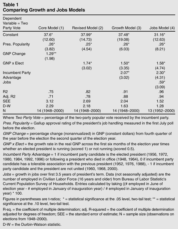
This core political economy model, V=f(P, G), is estimated (OLS) in column 1 of Table 1, for the election series 1948–2000. While by usual standards of political science explanation the supporting statistics (i.e., significance tests and goodness-of-fit) are good, they are not generally good enough to yield ex ante forecasts of sufficient accuracy. Therefore, as tests, in the past we have judiciously added other variables to the core model. These variables were selected on grounds of theory, and usually introduced into the model one at a time. After the 2000 forecast error, we did extensive testing of this sort, including potential independent variables from the following theoretical categories: the campaign, the economy, party politics, ethics, and institutional factors (Lewis-Beck and Tien 2002, 173). None of the variables measuring the campaign, the stock market, the presence of Ralph Nader, or the ethics of the Clinton administration managed statistical significance at conventional levels (Lewis-Beck and Tien 2002, Table 4, 180). What did seem to matter, however, was the time dimension of economic voting, and the institutional features of incumbency, discussed below.
First Revision: The Time Dimension of Economic Voting
Classic economic voting theory says electors punish the president's party when the economic record has been bad (Kiewiet 1983). But revisionist work indicates that electors will also punish the president's party when there is the promise of a poor economic future (Clarke and Stewart 1994). In other words, economic voting can be prospective, as well as retrospective. Before the 1996 contest, to incorporate this theoretically compelling result, we added a prospective index based on Gallup questions such as: “Which party—the Republican or the Democratic—will do a better job of keeping the country prosperous?” (Lewis-Beck and Tien 1996, 474). While conceptually sound, the measure was unfortunately empirically flawed, as became clear by the 2000 contest. For one, it was based on items not asked regularly. (Although the modal month for asking was August, they were not actually available in 2000 until October, which posed a grave problem of lead time.) For another, the presence of this prospective index in the 2000 model actually generated a worse forecast for 2000 than did the core model alone (Lewis-Beck and Tien 2001, 22).
The question became how better to incorporate the economic voting time dimension. Fortunately, independent work we were doing on national economic voting, using a pooled cross-section of American National Election Studies from 1956–1996, provided us with the critical clue (Nadeau and Lewis-Beck 2001). That study demonstrated that when an elected president himself was running for election, economic voting was largely retrospective. But, when the incumbent party candidate was not the president, economic voting was largely prospective. A president is judged mostly on his record, while a candidate of the president's party is judged mostly on his promises. This finding would seem to help explain Gore's failure to gain much from strong economic performance under the Democratic administration. He was not the president, and so benefited less from the economic boom.
In other words, the economic growth variable should be modeled as an interactive (G×E) term, rather than an additive term (G), since its impact depends on whether the incumbent candidate is the president or not (E). Based on our estimates from the 1956–1996 election survey pool, the impact of economic growth on the vote would be about cut in half if the candidate were not himself the president (Nadeau and Lewis-Beck 2001, 171). Therefore, to construct the interaction term, we multiplied G times E, where E is scored “1” if the elected president is running and “.5” otherwise. This revised model, V=f[P,(G×E)], is estimated in column 2 of Table 1. One observes that the relevant statistics are much improved, generally supporting the theory. Further, the model generates an out-of-sample forecast (from 1948–1996) for Gore of 54.9%, down from the 56.7% of the core model (Lewis-Beck and Tien 2001, 22).
Second Revision: The Advantages of Incumbency
Incumbency does have its disadvantages. It has been generally observed that long-standing governments lose votes, paying the “cost of ruling” (Paldam 1986). These “costs of ruling” might eventually spell “time for a change,” as Abramowitz (1996) describes the feelings of voters after a party has served two terms in the White House. Indeed, incumbency itself prescribes its own undoing in the U.S. presidential system with a two-term limit. But as long as the president, or his party, occupies the Oval Office, the advantages of incumbency—media access, resources, prestige—are there to exploit.
We imagine that the greatest incumbency advantage accrues to an elected president running for reelection (1956, 1972, 1980, 1984, 1992, 1996). Such a candidate stands at the head of his nation and party, and has had the experience, exposure, and opportunities of years in office. (The same can be said of those presidents running who came to the office through the death of an elected president, as in 1948 and 1964.) At the other extreme, the powers of incumbency are weakest when the party candidate is not the president and does not have the backing of the president. There are three cases of this type: 1960, 1968, 2000. Eisenhower's disdain for Nixon in 1960 was well-known, as was Johnson's disdain for Humphrey in 1968 (White 1961; 1969). With respect to 2000, the split between Gore and Clinton, largely of Gore's own doing, was widely publicized. In such a circumstance, the incumbent candidate lacks traditional, important sources of support, and would be expected to suffer accordingly at the ballot box. Between these two extremes are the cases where the party candidate is not the president, but relations between the two men are more or less tolerable (1952, 1976, 1988).
This trichotomous Incumbency Party Advantage variable, (labeled I and scored +1, 0, –1) is added to the above revised model, taking the form V=f[P,(G×E), I]. That model is estimated in column 3 of Table 1. Observe that it is easily statistically significant, and suggests that for each increment of incumbency advantage the party in the White House can expect an additional two percentage points toward the popular vote. Overall, the model statistics improve dramatically. The adjusted R-square goes up 14 points, and the standard error of estimate drops by over one-half a point. Most importantly, for our purposes, the residual for the 2000 prediction is just 2.34 percentage points, off the mark by only about one standard error. Theoretically, this is an extremely important result, for it suggests that the apparently idiosyncratic Gore debacle can be explained by general electoral forces in the American political system. Forecasting models of a systematic sort, such as this, do not yet appear ready for the scientific junkheap.
Last Revision: The Jobs Experiment
Most forecasting models include a measure of the economy, but there is no consensus on which one measure to use. There are objective indicators available, such as unemployment, GNP, GDP, or inflation. And, there are subjective indicators on hand, built from survey measures of consumer confidence about pocketbook and nation. In our forecasting work, we have stuck with GNP. The latest version of that model appears in column 3, Table 1, and we call it a Political Economy-Growth model to emphasize the role GNP plays. However, the inclusion of one particular economic variable in a forecasting model is a short-hand. Partly, this short-hand is forced on us by the limited number of degrees of freedom. We have said elsewhere that “these models should have no more than three independent variables” (Lewis-Beck and Tien 2002, 186). But, we have also argued that individual voters look at various aspects of the economy, and weight them differently, before arriving at a summary judgment about how the economy is doing (Nadeau and Lewis-Beck 2001). It is perhaps, then, worth exploring whether another economic variable, or some combination of economic variables, can be profitably added to the mix.
We have been led to experiment with a variable that has hitherto been unstudied in the election forecasting world—jobs. Our interest was sparked by the current controversy over job growth, or its relative lack, under the Bush administration. Economist Paul Krugman (New York Times, April 9, 2004, p. 19) has argued that “this year's election will be a contest between a candidate who advocates a return to economic policies that were associated with eight years of very solid job growth, and one who advocates continuation of policies that have, after three years, yielded exactly one good monthly jobs report…. If the election is driven by economics at all … it will reflect the job situation on the ground, which remains grim.” In more guarded commentary, a reporter in The Economist_(June 12, 2004, p. 27) questioned the “jobless recovery” and drew a parallel with 1992, when “George Bush senior lost the 1992 election during a lackluster, job-scarce recovery.”
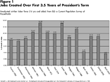
In Figure 1, one can see the cumulative job gains (in percent) for each presidential administration, measured from its inauguration to the end of June, six months before the election. (Data not available before 1952.) Looking at past administrations, the poorest job numbers occurred under George H. W. Bush, when jobs grew by only 4.40 percentage points over the term. Under the current administration, jobs have grown by 3.67 percentage points, an even lower number. These results force the question: Will George W. Bush meet the same fate as his father, becoming a one-term president?
Jobs Created Over First 3.5 Years of President's Term
When this Jobs variable is included in our forecasting model—V=f[P,(G×E), I, J]—the estimates change, as can be seen from column 4 of Table 1. The Jobs coefficient is clearly statistically significant, suggesting that for every percentage point rise in jobs, the presidential party can expect about another half-point of the popular vote share. Compare to the Growth model in column 3. All the other coefficients are stable in magnitude and their significance levels increase. Further, the adjusted R-squared jumps 6 points, and the standard error of estimate drops another half-point.1
The jobs model does not include 1948 as data on job growth from the household survey is not available for this year. To test the possibility that the improvement in the fit statistics in the jobs model is due to excluding the 1948 case, we ran the core and growth models without the 1948 case. The fit statistics for the core and growth models do not change much when the 1948 case is dropped.
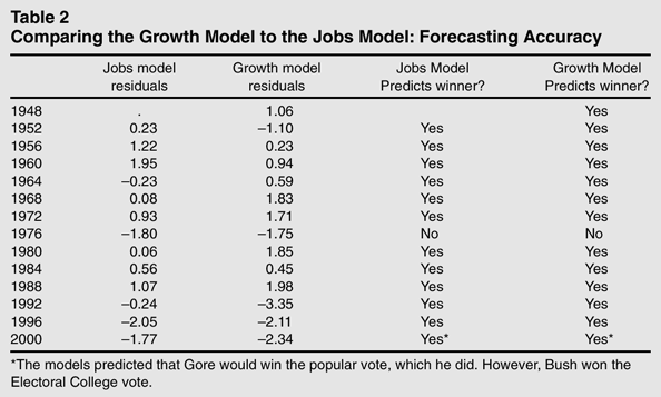
But, how robust are these results? We ran a series of diagnostic tests—studentized residuals, Cook's D, DFBETAs among them—and detected no troublesome signals, in particular no reasons to suspect the 2004 observation. In
Table 2 the actual residuals from this Jobs model (column 4,
Table 1) are compared to the Growth model (column 3,
Table 1). One observes no unusual pattern of residuals. Note further that, according to these within-sample results, the Jobs model predicts the 2000 election better than the Growth model does.
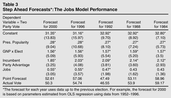
We test the Jobs model with further experiments. Table 3 presents step-ahead forecasts from the Jobs model, going back to 1984. One observes that, out-of-sample, the Jobs model manages to forecast the 2000 result with only 2.6 points of error. It also fares well for earlier elections, doing very well for 1992. The Jobs variable's increase in statistical significance in the more recent elections hints that perhaps the Jobs variable has become more and more salient for the electorate. Its increased potency is also suggested by a small but growing body of work that sees job insecurity emerging as a key variable in economic voting (Lacy and Mughan 2002).
Forecast for 2004: Too Close to Call?
We have observations on our independent variables as of August 27, 2004: P=47, G×E=1.32, I=1, J=3.67. Plugging these scores into the jobs model forecasts just 49.93% of the two-party popular vote for President Bush. Strictly speaking, then, the forecast is a two-party popular vote win for Senator Kerry. However, the margin of error must be considered. The standard error of estimate is 1.52. The suggestion is that Bush could lose (or win) by a hair, i.e., [49.93 ± 1.52]=[48.41, 51.45]. Taking this plausible amount of error into account, the race is too close to call.
From Popular Vote to Electoral Vote: 2004 Mirrors 2000?
It is the electoral vote, not the popular vote, which ultimately counts in winning the presidency. Fortunately, the two variables are very highly related, r=.97 (Lewis-Beck and Tien 2002, 178). (If popular vote is measured as percentage of the total vote, instead of two-party vote, r=.92.) Further, as a rule of thumb, if a candidate's popular two-party vote share exceeds 50%, then he or she can expect to win. However, that rule is only an approximation. When this popular vote share falls just a small amount above the “magic number” of 50%, then the regression prediction is that the candidate will not gain a majority of the electoral vote, even with this popular vote majority.2
The fact that the popular vote share is highly, almost perfectly, predictive of the electoral vote share suggests that the set of presidential election rules is generally democratic. Increases in the popular vote (the votes of the people) reliably translate into increases in electoral vote. However, there is a small “undemocratic window” that occurs when the two-party popular vote share falls between 50%–51%. Any popular vote share in that one percentage point region yields a prediction (from Eq. 1) of an Electoral College defeat, despite the winning of the popular vote majority. Fortunately, the probability of this “undemocratic” occurrence is small, but it is not zero, as the 2000 election demonstrated.
Of course, this was the bitter experience of Al Gore in 2000, when he received 50.3% of the two-party popular vote.
When electoral vote (EV) share is regressed (OLS) on two-party popular vote (PV) share, N=14 (1948–2000), the following equation, R-squared=.94, SEE=7.42, results (Lewis-Beck and Tien 2002, 177):
Plugging in the actual Gore popular vote outcome yields the following prediction:
Plugging in our Bush 2004 popular vote forecast yields the following prediction:
Thus, the electoral vote forecast literally agrees with the popular vote forecast, in that both say Bush will lose. But, as with the popular vote forecast, we see that the margin is extremely close. If the electoral vote forecast were off one standard error of estimate (at 7.42 percentage points), then Bush could win. Using that one standard error of estimate, it is plausible that the actual electoral vote share in percent could be [44.75 ± 7.42], for a confidence interval of [37.33, 52.17]. Again, one suggestion is that the race is too close to call.
Another suggestion from these results is dramatic. If the Bush two-party popular vote share falls between 50–51 percent, the electoral vote prediction from Eq. 1 above is that he would lose. (See also footnote 2). Then, we would have a situation where the incumbent party won the popular vote but lost the electoral vote. Eerily, it seems just possible that 2004 might be a repeat of 2000.
Conclusions
The exercise of forecast modeling merits continued pursuit. The anomalous 2000 outcome can be explained, if not explained away. Analysts do not have to resort to ad hoc, idiosyncratic, contest-specific characteristics in order to account for the large Gore vote deficit. The general electoral theory provided by the Political Economy-Jobs model covers the case well. Since Gore was not himself president, his candidacy could not take full advantage of the Democratic incumbency, which oversaw a GNP boom. His actual estrangement from the leader of the party caused his campaign fortunes to sink further. On top of this, seven of the last 10 administrations had actually created jobs at a rate greater than in the 1996–2000 period, further undercutting his Democratic vote base. Seen in this light, small wonder that Gore did not do better.
What does the Jobs model spell for 2004? The president himself is running, and to him accrue the electoral benefits of incumbency, including the ability to take advantage of the current positive rate of economic growth (2.64 annualized.) However, these benefits are offset, first, by his limited popularity and, second, by his poor record of job creation. His mediocre popularity score undoubtedly reflects widespread dissatisfaction with the Iraq War and his direction of it. With respect to jobs, his administration has the dubious distinction of delivering the poorest performance of the post-World War II period. There is growing evidence that voters pay attention to this type of economic indicator. It appears to have helped do in his father in 1992, and may well do him in as well. However, these negative forces—weak popularity and poor job creation—must be balanced against the positive forces—incumbency and economic growth. Taken together, these conflicting forces place the race on the razor's edge. The model, technically speaking, predicts a paper-thin defeat for President Bush. If that were to happen, which it may well not, he would follow in his father's footsteps and for much the same reasons.
We wish to thank economist George Neumann, University of Iowa, for his suggestions about measuring job growth. Of course, any errors we made in that measurement are our own responsibility.