
I. INTRODUCTION
During its service period, an aircraft is subject to different loads and environments. Reference Barter and Molent1 The alternating load may, in the long run, cause fatigue fracture of the structure; at the same time, the environment may lead to corrosive damage. Reference Borrego, Costa, Silva and Ferreira2,Reference McNaughtan, Worsfold and Robinson3 One of the characteristics of military aircraft service is that more than 95% of its service time is parked at the airport and less than 5% is on duty or training in the air. Reference Dan, Muto and Hara4 When parked, the main damage to the aircraft structure is corrosion due to environmental. Reference Zheng, Yu, Gao and Jiang5 When flying in the air, the main damage is fatigue due to the alternating load. Reference Zupanca and Grum6 At present, the common method to forecast the service life of aircrafts in the USA is to carry out tests on the specimens under different load/environment spectra. Reference Jiang, Tian and Zhou7 The load spectrum simulates flying condition in the air, whereas the environmental spectrum simulates parking condition in the airport. The total time in which the aircraft is undergoing corrosion-fatigue cycles represents its service life. There are some environmental spectra now in China that apply to coastal areas, Reference Li, Liu and Jia8–Reference Alexopoulos, Dalakouras, Skarvelis and Stavros10 and they are always refereeing to the part of Subtropical Coastal Areas and the Structure Covered by Coating (CASS) designed by the U.S. Air Force to adapt to subtropical coastal areas. Reference Miller and Schuessler11 In the CASS, one corrosion test cycle is equivalent to one year of corrosion on the ground. For example, 192 h dry–wet cyclic immersion corrosion in the lab corresponds to one year corrosion in coastal areas. But in reality, the aircraft is on duty frequently, and it not parking in the airport one year and flying in the air one year. So, using one-year corrosion spectra and one-year load spectra to forecast the service life is existed deviation to the practical condition. Reference Liu, Li and Jia12 So, the service life obtained by such one year environment/load spectrum would be conservative. Now there are few reports focusing on the difference of the forecasting service life between using one-year corrosion spectra and XX-mouth corrosion spectra. At the same time, corrosion damage is a cumulative process and the rule of fatigue life decreases as corrosion time increases is very important. Reference Crawford, Loader, Liu, Harrison and Khan Sharp13 In addition, the structural components of airplanes have different sizes, exhibiting different fatigue performance even though tested under the same stress conditions. Reference Wang, Xiong, Shenoi, Liu and Liu14 Generally, larger specimens have shorter fatigue life than smaller specimens, because large specimens contain more flaws and crack initiation life is short. But, there are few papers paying attention to the fatigue life of different size specimens after corrosion.
In this work, three factors on the fatigue life of 7B04-T6 aluminum alloy are explored: corrosion time, corrosion/fatigue alternation frequency (maintaining 192 h of total corrosion time for all tests) and specimen size (two specimen sizes are investigated). The mechanism of action is discussed. The results could provide a reference when designing the load/environment spectra for service life forecasting.
II. MATERIALS AND EXPERIMENTS
A. Materials and chemicals
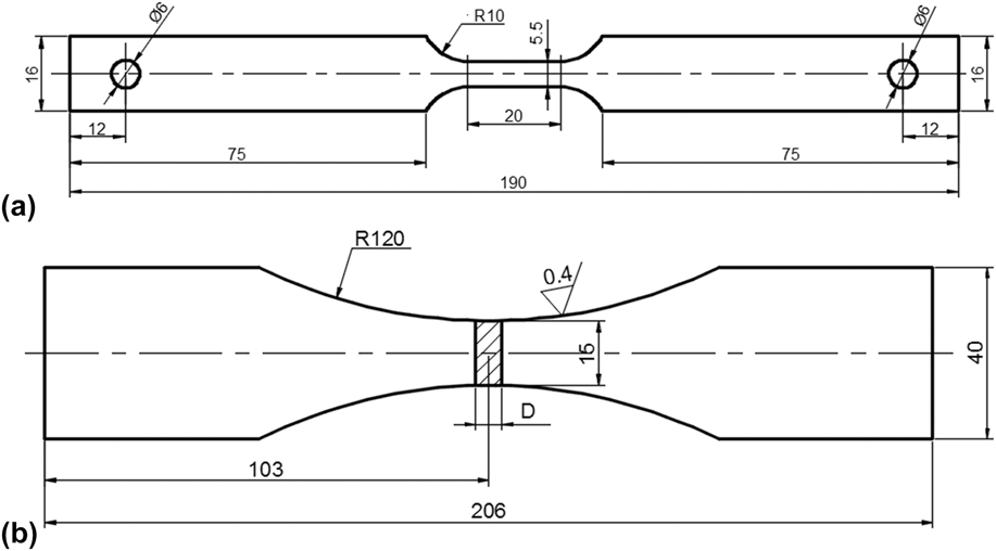
AA7B04-T6 was supplied by Chinalco (Beijing, China). The thickness of the AA7B04-T6 plate was 3 mm with a chemical composition of 6.0 wt% Zn, 2.5 wt% Mg, 1.5 wt% Cu, 0.15 wt% Fe, 0.5 wt% Mn, 0.1 wt% Si, 0.05 wt% Ti, and balance Al. The mechanical properties of the material were: yield strength (YS) of 537 MPa, tensile strength (TS) of 596 MPa, and 11% elongation. Figure 1 shows a schematic diagram of the specimen’s geometry. Before testing, all specimens were polished using 200#, 400#, 600#, 800#, 1000# grit alumina paper in sequence. The specimens were then degreased with acetone and rinsed with deionized water. Finally, all specimens were dried with clean compressed air.
Specimen dimension.

B. Influence of precorrosion time
The influence of precorrosion time was tested using specimens shown in Fig. 1(a). The precorrosion process consisted in the dry–wet cyclic immersion corrosion. The environmental conditions were as follows: 5% NaCl, pH 4 (adjusted by adding 10% NaOH and 20% H2SO4), 40 °C, relative humidity (RH) of 95%. The information of corrosion time and the solution was obtained from CASS. Each dry–wet cycle lasted 30 min: 7.5 min for immersion and 22.5 min drying in air. The pre-corrosion times were 6, 12, 24, 48, 96, and 192 h. After dry–wet cyclic corrosion, fatigue tests were carried out using constant amplitude with σmax = 150 MPa and R = 0.06 (we choosing this σmax = 150 MPa is according to the S–N curve and under this stress the fatigue life is about 12 × 104 after 192 h corrosion). And when the fatigue life is reached 1 × 10⁶ cycles, the test is stopped. In this test, we use the high frequency fatigue tester. Three specimens were tested in each condition to assure reproducibility.
C. Influence of specimen’s size
In this test, two dimensions’ specimens, as shown in Figs. 1(a) and 1(b), were used (usually, the specimen’s size in the laboratory test is small, but the actual structure is always large. So, it is necessary to study the fatigue behavior with different sizes after corrosion). The pre-corrosion step consisted in the dry–wet cyclic immersion corrosion, as described in Sec. II. B. Pre-corrosion times of 48, 96, and 192 h were chosen. After dry–wet cyclic immersion corrosion, fatigue tests were carried out. Once again, constant amplitude, σmax = 150 MPa, and R = 0.06 were used. Three specimens were tested in each condition to assure reproducibility.
D. Influence of corrosion/fatigue alternation frequency
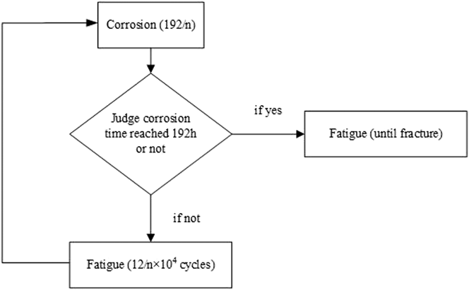
In this test, the specimen shown in Fig. 1(a) was used. We referenced the CASS and collected the environmental data of coastal areas to design environment spectra. The corrosion factors were as same as those described in Sec. II. B. 192 h of corrosion in the laboratory were equivalent to one year of corrosion in the coastal areas. Accordingly, 16 h of corrosion in laboratory equaled one month of corrosion in the coastal areas. After 192 h of corrosion, the fatigue life of AA7B04-T6 is 122,632 cycles. Therefore, one-month fatigue life corresponds to about 1 × 10⁴ cycles. A schematic representation of the experimental flow is shown in Fig. 2.
Experiment flowchart.

Four different alternation frequencies were investigated—with one, two, four, and six cycles. From here on, “n” will be used to indicate the number of cycles. For example when n = 1, it represents the situation in which the specimen was continuously exposed to corrosion for 192 h, followed by fatigue tests until it fracture (this test correspond to one-year environment spectrum)—corrosion 192 h + fatigue until break; when n = 6, it represents that the corrosion process was carried out in six steps (each step was 32 h corrosive and corresponding to a two-month environment spectrum), and fatigue tests of 2 × 10⁴ cycles were carried out until fatigue fracture—corrosion 32 h + fatigue 2 × 10⁴ + corrosion 32 h + fatigue 2 × 10⁴ + corrosion 32 h + fatigue 2 × 10⁴ + corrosion 32 h + fatigue 2 × 10⁴ + corrosion 32 h + fatigue 2 × 10⁴ + corrosion 32 h + fatigue until fracture.
Three specimens were tested in each condition to assure reproducibility. The total and residual fatigue lives were compared and an analysis was carried out on the effects of the corrosion/fatigue alternation frequency.
III. RESULTS
A. Fatigue life after different pre-corrosion times
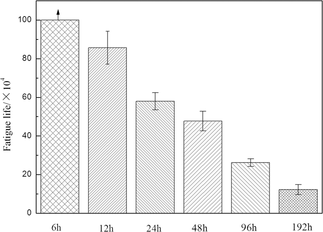
The fatigue life after different corrosion times is shown in Fig. 3. After 6 h corrosion, the fatigue life was longer than 1 × 10⁶ cycles. As corrosion time increased, fatigue life decreased. Comparing the results obtained for the specimen subject to corrosion for 12 h (fatigue life after 6 h corrosion is longer than 1 × 10⁶), the fatigue life of specimens exposed to corrosive conditions for 24, 48, 96, and 192 h, decreased by 32.32%, 60.26%, 78.47%, and 89.88%, respectively. After fitting, the relationship between fatigue life and corrosion time was described through an exponential correlation:
 $${N_{\rm{f}}} =\; \left[ {161.3\,\exp {{ - {\rm{time}}} \over {971.3}} + 119.2\,\exp {{ - {\rm{time}}} \over {12.9}} - 120} \right] \times {10^4}\quad .$$
Influence of the pre-corrosion time for AA7B04-T6 fatigue life.

From this equation, we could get the fatigue life of AA7B04 after the different time corrosion. Such as the aircraft was parking in this place one month (equal the corrosion time 16 h), the residual fatigue life was about 731,477 cycles. This residual fatigue life could guide the actual flying time.
B. Fatigue life after different corrosion/fatigue cycles
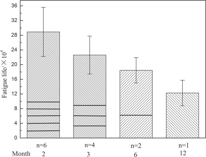
The influence of corrosion/fatigue alternation frequency is shown in Fig. 4. With the increase of corrosion/fatigue alternation frequency, the fatigue life of AA7B04-T6 increased. It was 136% (six cycles), 84.4% (four cycles), and 56.4% (two cycles) longer than the one observed in the one corrosion/fatigue cycle. This indicates that the estimate of the service life of an aircraft, carried out considering a one-year environmental spectrum, is conservative and that the actual service life is higher than the one forecasting.
Influence of corrosion/fatigue alternate frequency.

After fitting, the relationship between environment spectrum (test month) and fatigue life was found to be:
 $${N_{\rm{f}}} = \left[ {25.52\,\exp \left( {{{ - {\rm{mouth}}} \over {5.43}}} \right) + 9.56} \right] \times {10^4}\quad .$$
This relationship could be used to correct the existing forecasting life, which was obtained by using one-year environment spectrum. Such as the aircraft was flying once in a month, we could get the fatigue life from this equation was about 307,875 cycles and the actual service life was about much longer than the forecasting life.
C. Fatigue life of different sized specimens after pre-corrosion
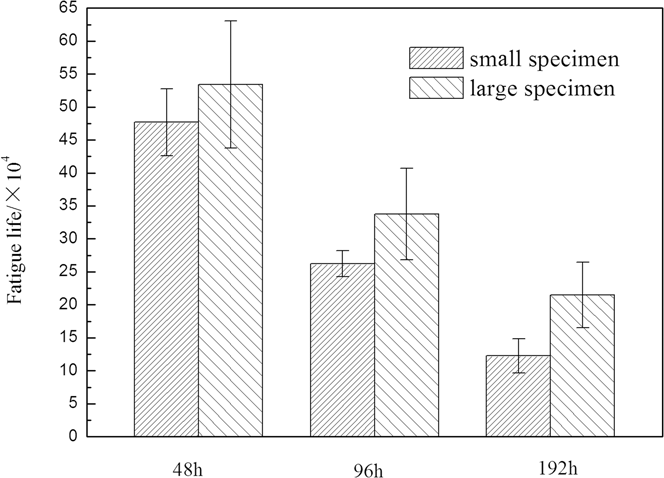
The fatigue life of different sized specimens after different pre-corrosion times is provided in Fig. 5. As shown in Fig. 5, with the extension of corrosion time, fatigue life decreased no matter how large the specimens were. However, for a given corrosion time, the fatigue life of larger specimens was higher than the corresponding value for smaller specimens. The increase in fatigue life from small to big specimens was of 11.99% for 48 h corrosion, 28.77% for 96 h corrosion, and 75.23% for 192 h corrosion. In addition, the influence of corrosion time for small specimens was stronger than for large specimens. For example, when corrosion time increased from 48 h to 96 h and 192 h, the fatigue life of small specimens decreased by 38.77% and 75.23%, respectively, whereas for large specimens it decreased by 36.79–58.76%.
Fatigue life of different size specimens after different time pre-corrosion.

IV. DISCUSSION
During the fatigue process, the fatigue life could be divided into two sections: one is the initiation stage; the other is crack propagation stage. The cracks usually appear in the material surface, such as gap, tool mark, or corrosion pits. So, the appearance of corrosion pit would reduce the crack initiation life and the more serious of the corrosion, the less of the crack initiation life. Reference Burns, Kim and Gangloff15 At the same time, the distribution of corrosion pits had a strong impact on the fatigue crack spreading behavior. These pits can change the path of fatigue crack propagation. It reflects the fact that the fatigue crack propagation direction and path are closely dependent on the competition result between corrosion pit size and the interface strength of grain. Reference Xu-Dong, Xi-Shu, Huai-Hui, Yin-Long and Zhi-Tao16 So, the larger the corrosion pit, the lower of the fatigue life.
A. Influence of pre-corrosion time
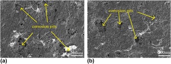
The surface topographies of AA7B04-T6 after different pre-corrosion times are provided in Fig. 6. It can be seen that with the extension of corrosion time, the corrosion degree increased. After 6 h corrosion, there were few and shallow pits on the surface of the specimen [Fig. 8(a)]. When the corrosion time was extended to 12 h, the pits became numerous and their morphology became evident [Fig. 6(b)]. After 48 h corrosion, deep and large pits appeared [Fig. 6(c)]. After 192 h corrosion, the situation became very serious [Fig. 6(d)]: the surface was completely corroded and most of the substrate materials had peeled off. At the same time, large and deep pits were evident on the surface. Reference Cui, Liu, Zhang and He17
Surface topographies of AA7B04-T6 after different corrosion: (a) 6 h, (b) 12 h, (c) 48 h, (d) 192 h.

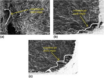
The fracture morphologies of AA7B04-T6 after different corrosion times are shown in Fig. 7. In all the tests, it was clear that the reason for fatigue cracking has been the corrosion pits Reference Pao, Gill and Feng18 ; therefore, the corrosion damage would decrease the fatigue crack initiation time and lead to a decrease in fatigue life. With the extension of corrosion time, the pit area became increasingly larger and the corrosion degree became more serious.
Fracture topographies of AA7B04-T6 after different time corrosion: (a) 12 h, (b) 48 h, (c) 192 h.

B. Influence of corrosion/fatigue alternation frequency
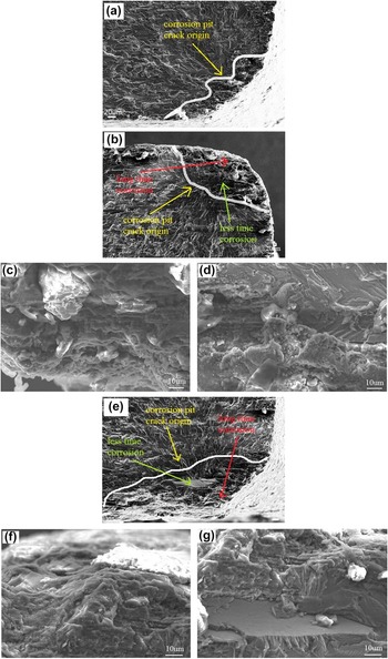
The fracture morphologies using different environment spectra are provided in Fig. 8. Figure 8(a) refers to the use of the one-year environment spectrum (n = 1), Figs. 8(b)–8(d) refer to the three-month environment spectrum (n = 4), and Figs. 8(e)–8(g) refers to the two-month environment spectrum (n = 6). It was clear that the reason for fatigue cracking was the formation of the corrosion pits. With the decreased in the value of n, corresponding to increased corrosion-fatigue cycles, the corrosion pit area increased, [by comparing Figs. 8(a), 8(b) and 8(e)]. The width of pit in Fig. 8(a) was 215 μm and the depth was 38 μm; in Fig. 8(b) the width was 218 μm and the depth was 84 μm; in Fig. 8(e) the width was 402 μm and the depth was 91 μm. The corrosion pits presented two kinds of morphologies, moving from the outside toward the inside. On the outside of the corrosion pits, most matrixes were destroyed [Figs. 8(c) and 8(f)]; but inside the pits, corrosion had been lighter and some areas were flat [Figs. 8(d) and 8(g)]. This was due to the fact that the outer part of the pits had suffered long time corrosion, but the inside had been corroded only in the last corrosion cycle.
Fracture morphology of different cycles’ specimen: (a) n = 1; (b–d) n = 4; (e–g) n = 6.

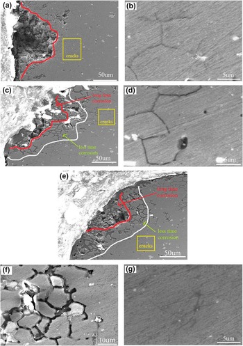
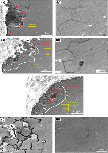
Cross section morphologies using different environment spectra are shown in Fig. 9. It was clear that there were large pits in the AA7B04 specimen after corrosion. Two kinds of morphologies appeared in Figs. 9(c) and 9(e): serious corrosion in the outer part of the pits and mild corrosion in the more inner regions. Under the bottom of corrosion pits, different phenomena were observed. Figure 9(b) shows the presence of small cracks under the bottom the corrosion pits and the cracks were sharpened. In Fig. 11(d), there were also some cracks, but the cracks were thick. Finally, in Figs. 9(f) and 9(g), the corrosion channel was obvious and the small cracks disappeared. In other terms, with the decrease of n, the cracks under the corrosion pits became thicker and their curvature radius became larger. In addition, the cracking initiation life became longer, so the residual fatigue life increased (shown in Fig. 4).
Cross section morphology of different cycles’ specimen: (a and b) n = 1; (c and d) n = 4; (e–g) n = 6.

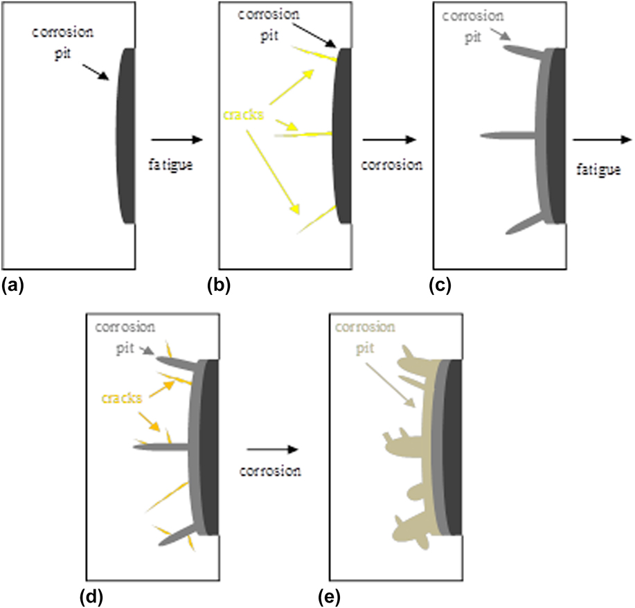
The morphological change of pits and cracks during the corrosion and fatigue process is provided in Fig. 10. Condition (a) was after corrosion, there were some corrosion pits appeared on the surface; then fatigue process was going (condition a–b), after that, according to cyclic loading, there were some cracks under the bottom of corrosion pits (condition b); then corrosion process was followed (condition b–c), on the one hand, corrosion pits became larger, on the other hand, the small cracks get bigger and curvature radius became larger (condition c); then the fatigue process was proceed (condition c–d), there were some new cracks (condition d); then corrosion process was suffered (condition d–e), the corrosion pits became larger and the cracks was corroded that curvature radius became larger (condition e)…In those corrosion-fatigue-corrosion…process, fatigue crack appear-disappeared constantly, so there were coarse corrosion channel obviously (shown in Fig. 9). The damage caused by fatigue process would be disappeared during the corrosion process, so the total fatigue life was high. The thick cracks had high cracking initiation life, so the residual fatigue life was high. Using two-mouth environment spectrum corroded, the fatigue life was much higher than using one-year environment spectrum no matter the total life or the residual fatigue life. Reference Jian, Daoxin, Zuoyan, Xiaohua, Yuting and Tengfei19
Sketch of cracks during the corrosion and fatigue process.

C. Influence of specimen size
The surface topographies of specimens of different dimensions after 192 h pre-corrosion are shown in Fig. 11. For these two specimens, the corrosion was very serious. Pits formed on the surface and, at the same time, most of the substrate materials were peeled off. A comparison of Figs. 11(a) and 11(b) indicates that the corrosion degrees of the two specimens are not quite different.
Surface topographies of different dimension specimens after 192 h pre-corrosion: (a) small specimen, (b) large specimen.

Figure 12 shows the fracture topographies of differently sized specimens after 192 h corrosion. It can be seen that in both conditions, the cracks originate at the corrosion pit. The size of the corrosion pits did not differ significantly for the two specimens, indicating that for the same corrosion time, the damage of the two specimens was same.
Fracture topographies of different dimension specimens after 192 h pre-corrosion: (a) small specimen, (b) large specimen.

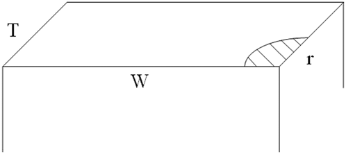
The specimen’s cross-sectional model after corrosion is shown in Fig. 13. W indicates the width of the specimen and T its thickness. On the basis of the results previously discussed it was concluded that the corrosion degrees of the two specimens having different dimensions were the same. Supposing the corrosion pit was rounded in correspondence of the specimen’s edge (see from Fig. 12) and indicating its radius was r. So, the area of this pit would be 1/4πr 2. When calculating the actual stress on the specimen’s cross-section, the stress concentration effect caused by corrosion pit was neglected.
Sketch of specimen’s cross section after the corrosion.

The actual stress on the cross-section (σactual) after corrosion can be expressed by Eq. (3). Where σ is the nominal stress used in the fatigue test (σ = 150 ΜPa), and W·T is the cross-sectional area. The overall applied load is therefore
 ${\sigma _0}WT/{1 \over 4}\pi {r^2}$
is the actual value of cross-sectional area.
 $${\sigma _{{\rm{actual}}}} = {{\sigma WT} \over {WT - {1 \over 4}\pi {r^2}}}$$
the value of T has been always maintained constant and equal to 3 mm. If we suppose the width of the small specimen W = A, and the width of the large specimen W = A′, the actual stress on the small and specimens may be evaluated as
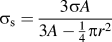 ${\sigma _{\rm{s}}} = {{3\sigma A} \over {3A - {1 \over 4}\pi {r^2}}}$
and
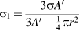 ${\sigma _{\rm{l}}} = {{3\sigma A'} \over {3A' - {1 \over 4}\pi {r^2}}}$
, respectively.
To compare the values of σs and σl, a new function Γ = σs − σl was introduced
 $$\Gamma = {{3\sigma A} \over {3A - {1 \over 4}\pi {r^2}}} - {{3\sigma A'} \over {3A' - {1 \over 4}\pi {r^2}}}\quad .$$
When corrosion did not take place, the value of r was equal to zero (r = 0). The differentiation of
 ${{{\rm{d}}\Gamma } \over {{\rm{d}}r}}$
gives
 $${{{\rm{d}}\Gamma } \over {{\rm{d}}r}} = {3 \over 2}\sigma \pi r{{\left( {A' - A} \right)\left( {9AA' - {1 \over {16}}{\pi ^2}{r^4}} \right)} \over {{{\left( {3A - {1 \over 4}\pi {r^2}} \right)}^2}}}\quad .$$
In this paper
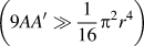 $\left( {9AA' \gg {1 \over {16}}{\pi ^2}{r^4}} \right)$
, so
 ${{{\rm{d}}\Gamma } \over {{\rm{d}}r}} > 0$
and the ? is a monotonically increasing function. When r = 0, Γ presents a minimum value at zero. When r > 0, Γ > 0, so σs − σl > 0 and σs > σl. Obviously, the actual stress on the small specimen was larger than the one on the large specimen, so the fatigue life of small specimen was shorter than that of the large specimen.
Fatigue spreading area and fatigue striation of different sized specimens are provided in Fig. 14 (the test area of fatigue striation was always of 400 μm from crack origin). It can be seen that the large specimen’s fatigue extension area [Fig. 14(b)] was bigger than small specimen’s [Fig. 14(a)] and the space between the adjacent fatigue striations of large specimen was smaller than the one observed for the small specimen at the same distance from crack origin [show as Figs. 14(c) and 14(d)]. The fatigue life of large specimens was thus higher than the one of small specimens, consistently with the results of Eqs. (3)–(5).
Fatigue crack initiation and fatigue striation of different size specimens after 192 time corrosion: (a and c) small specimen; (b and d) large specimen.

V. CONCLUSIONS
Three main conclusions may be drawn from the results of this work.
-
(1) After pre-corrosion, the fatigue life of AAB04-T6 decreased. Corrosion pits acted as the fatigue source, producing and extending fatigue cracks and reducing the fatigue life. As corrosion time was increased, fatigue life decreased. The relationship between fatigue life and corrosion time was:
 ${N_{\rm{f}}} = \left[ {161.3\,\exp {{ - {\rm{time}}} \over {971.3}} = 119.2\,\exp {{ - {\rm{time}}} \over {12.9}} - 120} \right] \times {10^4}$
. This equation could be used to forecast the residual fatigue life of AA7B04 after different time corrosion.
-
(2) Although the total time was the same, corrosion/fatigue alternation frequency had a significant influence on the fatigue life of AA7B04-T6. With the increase of alternation frequency, fatigue life increased. It was 136% (six cycles), 84.4% (four cycles) and 56.4% (two cycles) longer than the fatigue life measured for specimens subjected to a single corrosion/fatigue cycle. The relationship between fatigue life and the duration of the environment spectrum was:
${N_{\rm{f}}} = \left[ {25.52\,\exp \left( {{{ - {\rm{month}}} \over {5.43}}} \right) + 9.56} \right] \times {10^4}$
. This equation could be used to corrected the fatigue life of AA7B04 by using one year environment spectrum. This means that, when forecasting the service life, the environment spectrum must correspond to the actual service condition (parking/on duty frequency = corrosion fatigue alternate frequency). -
(3) The specimen’s size had significant influence on the fatigue life of AA7B04-T6. After the same corrosion time in the same environment, fatigue life of small specimens was shorter than fatigue life of large specimen. This was because the actual stress was different for the two specimens and the fatigue life of small specimens was more sensitive to the corrosion damage.


ACKNOWLEDGMENTS
The authors are grateful to the National Natural Science Foundation of China (Grant No. 51171154) and the National Defense Key Disciplines Laboratory of Light Alloy Processing Science and Technology, Nanchang Hangkong University (Grant No. gf 201401001).