Implications
The use of random regression models (RRM) utilizing B-spline functions can be an option to estimate genetic parameters for BW at distinct ages in meat-type quail, since these models present less issues when compared with Legendre polynomials. However, few studies applied RRM using B-spline functions to estimate genetic parameters for growth traits. The results obtained herein demonstrate that RRM using B-spline functions estimated variances and heritability estimates more appropriately. Therefore, these models provide a lower time for convergence, as well as less computational use in comparison with Legendre polynomials or multi-trait analysis.
Introduction
For several years, quail selection in Brazil aimed only at egg production and no commercial breeding program for meat-type quail was available. In this way, inadequate selection provides problems related to inbreeding resulting in reductions in productive traits (Caron et al., Reference Caron, Minvielle, Desmarais and Poste1990; Toelle et al., Reference Toelle, Havenstein, Nestor and Harvey1991; Marks, Reference Marks1996; Minvielle, Reference Minvielle1998). In this scenario, the genetic material of less productive potential becomes a problem when selection is focused on productive traits. Thus, when selection of economic-interest traits is based on a directed breeding program, changes on growth caused by the selection itself are more accurate and precise (Khaldari et al., Reference Khaldari, Pakdel, Yegane, Javaremi and Berg2010; Karaman et al., Reference Karaman, Narinc, Firat and Aksoy2014).
The selection of meat-type quail has been directed for BW since growth traits are of great importance, and it is easy to be measured (Barbieri et al., Reference Barbieri, Ono, Cursino, Farah, Pires, Bertipaglia, Pires, Cavani, Carreño and Fonseca2015; Buzała et al., Reference Buzała, Janicki and Czarnecki2015). In addition, the selection for BW responds quickly and has a correlated response specially with carcass traits (Khaldari et al., Reference Khaldari, Pakdel, Yegane, Javaremi and Berg2010; Karaman et al., Reference Karaman, Firat and Narinc2013; Mota et al., Reference Mota, Abreu, Silva, Pires, Lima, Bonafé, Costa, Souza and Martins2015b; Firat et al., Reference Firat, Karaman, Başar and Narinc2016; Narinç et al., Reference Narinc, Karaman, Aksoy and Firat2016). It is noteworthy to mention that the response to selection may be different when evaluating male or female quail (Alkan et al., Reference Alkan, Mendeş, Karabağ and Balcioğlu2009).
Several models have been used for genetic evaluation in breeding programs to evaluate repeated measurements on animals. Random regression models have been proposed as an alternative to genetic evaluate animals to assess longitudinal data more accurately (Schaeffer, Reference Schaeffer2004; Albuquerque and El Faro, Reference Albuquerque and El Faro2008; Boligon et al., Reference Boligon, Baldi and Albuquerque2011 and Reference Boligon, Mercadante, Lôbo, Baldi and Albuquerque2012). In addition, these models are a way of modeling the variances and covariances along a time period (Meyer, Reference Meyer2000, Reference Meyer2004 and Reference Meyer2005a). The RRM consider that the genetic and environmental effects associated with an animal are estimated as growth trajectory deviations of each animal relative to the average growth trajectory (Schaeffer, Reference Schaeffer2004). In contrast to the multi-trait models that provide predictions for specific points or ages, the RRM allow the prediction of breeding values for the growth curve as a whole, for each desirable age and for growth curve functions (Albuquerque and El Faro, Reference Albuquerque and El Faro2008).
The RRM are usually modeled using orthogonal Legendre polynomials, but other functions can be used as the spline functions, which use various segmented polynomials of low degree joined together in certain positions to model the curve (Huisman et al., Reference Huisman, Veerkamp and Van Arendonk2002), reducing the number of estimated parameters in RRM analyses. Considering the aforementioned, the objective was to estimate covariance functions for direct genetic and permanent environmental effects, and subsequently obtaining genetic parameters for growth traits in meat-type quail, using RRM with Legendre polynomials and B-spline functions, in addition to obtain trends and genetic gains.
Material and methods
Data
A database containing the complete pedigree information of 7000 meat-type quail with a total of 40 987 BW records measured at hatching (day 0), 7, 14, 21, 28 and 35 days of age was utilized. The data utilized in this study are from a meat-type quail (Coturnix coturnix) strain (LF1) that pertain to the Quail Breeding Program of the Federal University of Jequitinhonha and Mucuri Valleys (‘Universidade Federal dos Vales do Jequitinhonha e Mucuri’). In brief, the LF1 strain was derived from a commercial flock of which 200 sires and 400 dams (the heaviest quail) were selected and randomly mated for three generations. The LF1 strain was then established. After establishment, mating continued and the LF1 strain utilized in the present study was in the 8th generation focusing on BW selection.
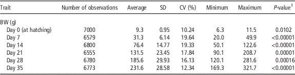
Contemporary groups were established including animals of the same generation, hatching and sex. All quail utilized in the present study were derived from hens of the same age. Analyses of data consistency and environmental effects for each trait were performed using the R software (R Development Core Team, 2015). When editing the data, animal records which were 3 SD above or below the average were excluded. Only animals with at least four records for BW and that pertained to a contemporary group with at least five individuals were kept for analysis. A summary of the data file composition after analysis consistency is depicted in Table 1.
Structure of the dataset utilized in the genetic evaluation of meat-type quail

Analyses
Models used to estimate genetic parameters included the direct genetic and permanent environmental effects as the random effect, and residual effects. Contemporary group were included as fixed effects. Hen was not considered as fixed effect because all quail utilized in the present study were derived from hens of the same age. Data were analyzed through animal model using random regression. Fixed and random regressions were represented by continuous functions in which animal age was fitted by orthogonal Legendre polynomials and by B-spline functions:
 $$y\,{\equals}\,Xb{\plus}Z_{1} a{\plus}W_{1} pe{\plus}{\epsilon}$$
in which y is the vector of observations, b the vector of fixed effects, a the vector of random coefficients for additive direct effects, pe the vector of random coefficients for permanent environmental effects, ɛ the vector of residual effects and X, Z 1, and W 1 are the corresponding incidence matrices to the fixed and random effects. The model was based on the following assumptions:
 $$\eqalign { E\,{\equals} & \left[ {\matrix{ y \cr a \cr {pe} \cr } } \right]{\equals}\left[ {\matrix{ {Xb} \cr 0 \cr 0 \cr } } \right]{;}\, {\matrix{ {\matrix{ } } \cr } } \cr \,V {\equals}& \left[ {\matrix{ {\matrix{ a \cr {pe} \cr } } \cr {\epsilon} \cr } } \right] {\equals}\left[ {{\rm }\matrix{ {K_{a} \,\otimes\,A} & 0 & 0 \cr 0 & {K_{{pe}} \,\otimes\,I_{{N_{A} }} } & 0 \cr 0 & 0 & R \cr } } \right]$$
in which K
a
and K
pe
are (co)variance matrices between random regression coefficients for additive direct and permanent environmental effects, respectively. A is the relationship matrix, I is an identity matrix, N
A
the number of animals which records are available,
 $\,\otimes\,$
the Kronecker product between matrices and R is a block diagonal matrix containing residual variances. Correlations between random regression coefficients for the different effects were set to 0.
The B-Spline function can be defined according to Meyer (Reference Meyer2005a) as base functions of degree P=0 assuming values of unit to all points in a given interval; otherwise, the value is 0. Quadratic (Q) and cubic (C) polynomials were considered for each individual segment of the base functions of degree P=2 and 3, respectively. Polynomials of the same degree were included in the model for all random effects. The m knots were chosen to divide the age in which animals were evaluated considering m−1 intervals equally spaced and the external knots were located on days 0 and 35. Direct additive genetic and permanent environmental effects were modeled using 2 to 4 segments.
A multi-trait analysis was also performed using a finite dimension model for BW at hatching, 7, 14, 21, 28 and 35 days of age. The model for all traits included the direct additive and residual effects as random effect. In addition, contemporary group and generation were included as fixed effects.
Covariance components
The covariance components and genetic parameters of the models were estimated by the restriction maximum likelihood method using the AIREML algorithm of the Wombat statistical package (Meyer, Reference Meyer2006). Direct additive genetic variances for BW at different ages
 $\left( {\hat{\sigma }_{{ai}}^{2} } \right)$
were obtained considering
 $$\hat{\sigma }_{{ai}}^{2} \,{\equals}\,f_{i}^{\prime} \Lambda _{A} f_{i} $$
in which
 $f_{i}^{\prime} $
is the vector of covariates corresponding to the B-spline functions of age in days, and
 $\Lambda _{A} $
is the matrix of direct additive genetic covariance between random regression coefficients. The genetic variances for the permanent environmental effects were obtained in a similar manner replacing
 $\Lambda _{A} $
by
 $\Lambda _{{PE}} $
which is the matrix for the permanent environmental effects between the random regression coefficients.
The residual variances
 $\left( {\hat{\sigma }_{{ei}}^{2} } \right)$
were considered to change according to age (described by four age classes). Thus, direct heritability of BW at different ages
 $\left( {h_{{ai}}^{2} } \right)$
was calculated using the equation:
 $$h_{{ai}}^{2} \,{\equals}\,{\raise0.7ex\hbox{${\hat{\sigma }_{{ai}}^{2} }$} \!\mathord{\left/ {\vphantom {{\hat{\sigma }_{{ai}}^{2} } {\hat{\sigma }_{f}^{2} }}}\right.\kern-\nulldelimiterspace}\!\lower0.7ex\hbox{${\hat{\sigma }_{f}^{2} }$}},\,{\rm in}\,{\rm which}\,\hat{\sigma }_{f}^{2} \,{\equals}\,\hat{\sigma }_{{ai}}^{2} {\plus}\hat{\sigma }_{{pei}}^{2} {\plus}\hat{\sigma }_{{ei}}^{2} $$
The same aforementioned equation was used to estimate the permanent environmental effect (pei
2) as a proportion of total phenotypic variances, replacing the numerator of this equation by
 $\hat{\sigma }_{{pei}}^{2} $
(Meyer, Reference Meyer2001; Mrode, Reference Mrode2005).
Comparison of models
Models with different polynomial order were compared using the Akaike information criterion (AIC; Akaike, Reference Akaike1974) and the Schwarz-Bayesian information criterion (BIC; Reference SchwarzSchwarz, 1978). The AIC and BIC consider the lack of fit and the number of parameters estimated in the model. The AIC can be used to compare models including the same fixed effects but with different variance structures whereas the BIC provides a similar assessment except that it attributes a higher penalty to models containing a greater number of parameters than the AIC. Statistical criteria were calculated as follows:
 $${\rm AIC}\,{\equals}\,{\minus}2\,{\rm log}\,L{\plus}2p$$
 $${\rm BIC}\,{\equals}\,{\minus}2\,{\rm log}\,L{\plus}p\,{\rm log}\left( {N{\minus}r} \right)$$
in which p is the number of parameters in the model, N the total number of observations, r the rank of the incidence matrix for the fixed effects in the model and log L is the logarithm of the likelihood function.
The results from the B-spline functions were compared with the best model obtained by random regression by using the orthogonal Legendre polynomials for the direct additive genetic and permanent environmental effects. The same fixed effects were considered for all RRM. In addition to the comparison of genetic parameters obtained through analysis of random regression and multi-trait models, direct responses to selection were predicted. In order to estimate the direct response to selection, it was used a selection intensity of 4% for males and 8% for females, and the following equation was used to estimate the direct responses to selection:
 $$GS_{x} \,{\equals}\,h_{x}^{2} {\times}i_{x} {\times}\sigma _{p} $$
in which GS
x
is the gain with the selection for the trait x,
 $h_{x}^{2} $
the heritability of the trait x, i
x
the selection intensity for the trait x and σ
p
the phenotypic SD of the trait x.
The models’ names utilized in this study were LEG, BSC and BSQ referring to models that utilized the Legendre polynomial, cubic B-spline and quadratic B-spline functions, respectively. Following the model name, there are two numbers: the first one corresponds to the residual variance, and the second one, to the degree of the polynomial (for the LEG models) and to the function (for the BSC and BSQ models).
Results and discussion
Descriptive statistics
The greatest number of measurements in the evaluated strain was for BW at hatching (Table 2). We observed little reduction in the other BW measurements, with values ranging from 93.9% to 96.86% of records remaining for the BW measured at day 35. These losses were because of mortality and tag losses from quail throughout their growth period.
Descriptive statistics for the data utilized in analyses of meat-type quail

1 P-value referring to fixed effect (contemporary groups).
The BW increased over the age, with a decrease in the growth rate after 28 days of age (Table 2). A similar pattern was reported by Rezvannejad et al. (Reference Rezvannejad, Pakdel, Miraee Ashtianee, Mehrabani Yeganeh and Yaghoobi2013). The average value for BW measured at 35 days of age was lesser than what reported by Silva et al. (Reference Silva, Ribeiro, Crispim, Silva, Bonafé, Silva and Torres2013) who evaluated meat-type quail. These differences in BW occur because of the differences of selection criteria between breeding programs. Thus, differences in performance of meat-type quail genotypes reflect genetic differences which may be a result of the number of selection generations, the selection intensity and nutritional level employed by the different breeding programs (Mota et al., Reference Mota, Coimbra, Abreu, Costa, Pires, Silva, Bonafé, Castro, Lima and Pinheiro2015a and Reference Mota, Abreu, Silva, Pires, Lima, Bonafé, Costa, Souza and Martins2015b). The SD presented higher values as the age advances. The CV were close throughout the evaluation period, demonstrating an association between the BW average and the SD. The CV values reported by Barbieri et al. (Reference Barbieri, Ono, Cursino, Farah, Pires, Bertipaglia, Pires, Cavani, Carreño and Fonseca2015) were similar those found in the current study.
Comparison of models
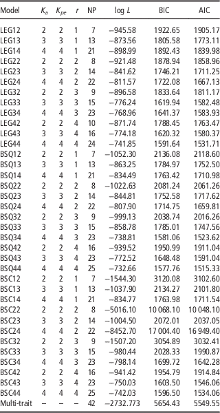
Both information criteria used to compare models (AIC and BIC) indicated that model BSQ44 best fitted the data structure. The Table 3 summarizes the results of the models’ comparison using the logarithm of the likelihood function (log L), BIC and AIC obtained for the models used to define the best variance structure of residual variances, and the orders of fit for additive genetic and permanent environmental effects. The number of parameters ranged from 7 to 25 in the evaluated models. Models’ evaluation criteria improved with the increase of the number of parameters for each evaluated model and residual variance class. However, the Legendre polynomials that considered variance homogeneity did not show this comportment. These results indicate a different behavior of the variance parameters for BW over the evaluated period, which requires a structure of heterogeneous variance to model such time dependency. Bonafé et al. (Reference Bonafé, Torres, Sarmento, Silva, Ribeiro, Teixeira, Silva and Sousa2011) and Gonçalves et al. (Reference Gonçalves, Pires, Pereira, Drumond, Felipe and Pinheiro2012) reported best data adjustment quality when utilizing the Legendre polynomial of sixth-order to evaluate BW of meat-type quail. We observed that the best adjustment to the structure of the components and (co)variances was obtained when polynomials of fourth-order and with four classes of residual variance were employed, showing lesser log L, BIC and AIC values, compared with models that considered homogeneity and smaller variances.
Comparison of models by likelihood logarithm (log L), Bayesian Information Criterion (BIC) and Akaike Information Criterion (AIC) for meat-type quail

k a =order of the covariance function to the direct additive effect; k pe =order of the covariance function to permanent environmental effects; r=number of classes for residual variances; NP=number of parameters; LEG=Legendre polynomial; BSQ=quadratic B-spline functions; BSC=cubic B-spline.
Among the evaluated models used to estimate the genetic parameters for quail BW, the model which considered quadratic B-spline functions with four classes of residual variance was the one that best fitted the average trajectory of growth (Table 3). According to Meyer (Reference Meyer2005a), when using the B-spline functions, it is possible to adjust low-degree polynomials in short segments of the trajectory of growth and, thus, to be more flexible when adjusting for seasonal fluctuations of animals’ growth.
Estimates of variance components
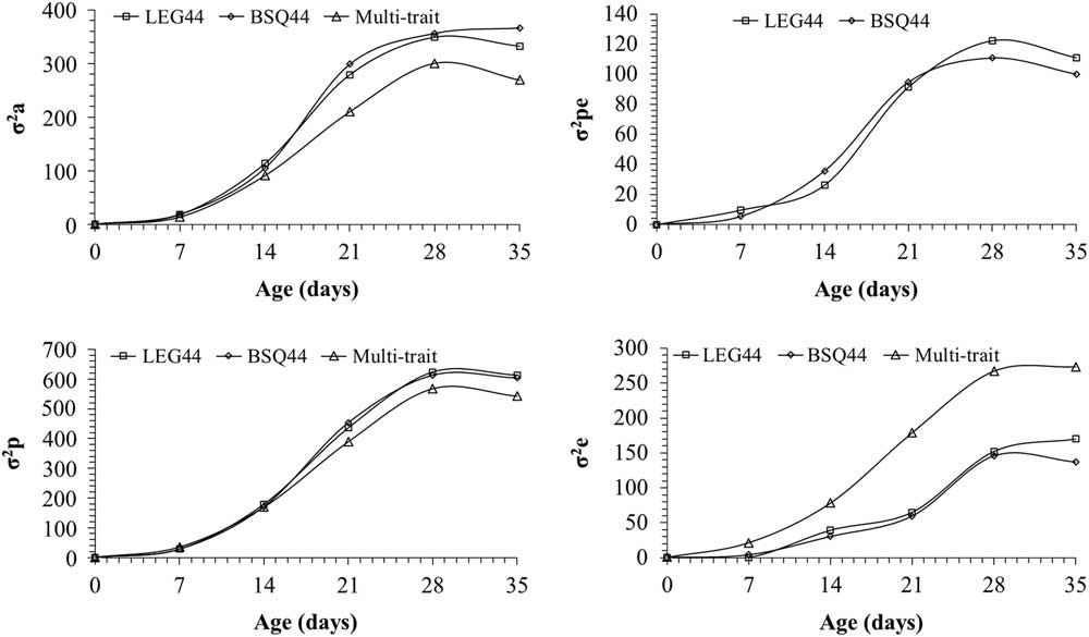
Phenotypic, direct additive genetic, and permanent environmental variances estimated by the models BSQ44 and LEG44 showed similar behavior until day 28, even increasing segments or the polynomial order (Figure 1). It should be highlighted that, in the case of B-spline functions, the best data adjustment depends on the order of segments to model the data structure, with issues especially when the data is irregularly distributed. The RRM, by considering the changes in the average and in the variance of the trait at different ages, as well as estimating the covariance between the points of the trajectory using covariance functions, allow to accurately model the covariance structure of the trait in comparison with multi-trait models (Meyer, Reference Meyer2004 and Reference Meyer2005b).
Estimates of the direct additive genetic
 $\left( {\sigma _{a}^{2} } \right)$
, permanent environmental
 $\left( {\sigma _{{pe}}^{2} } \right)$
, residual
 $\left( {\sigma _{e}^{2} } \right)$
and phenotypic
 $\left( {\sigma _{p}^{2} } \right)$
variances components obtained from LEG44 (□) and BSQ44 (◊) models, and by multi-trait analysis (∆). LEG=Legendre polynomial; BSQ=quadratic B-spline functions.

The RRM using B-spline functions seem to be a valuable tool for estimating genetic parameters for growth traits in meat-type quail, being directly comparable with those obtained in multi-trait analysis when knots are specified in standard age.
We observed that the genetic variances increased until day 28 and decreased at day 35 (Figure 1). Similar results were reported by Akbaş et al. (Reference Akbaş, Takma and Yaylak2004), Dionello et al. (Reference Dionello, Correa, Silva, Corrêa and Santos2008) and Bonafé et al. (Reference Bonafé, Torres, Sarmento, Silva, Ribeiro, Teixeira, Silva and Sousa2011). These authors observed that the variances also presented a trend to increase with age. The LEG44 model, on the other hand, presented a reduction of the residual variance at day 35 trending near 0 (Figure 1). According to Meyer (Reference Meyer2005b), high-order Legendre polynomials attribute too much emphasis on the range extremes’ information, resulting in unrealistic estimates of the (co)variances components of these extremes and difficulties in adjusting the uniformity along the curve. These results indicated that the inclusion of random regression coefficients for these effects allowed differentiating the estimated variances along the growth trajectory, evidencing those continuous functions must be employed to model them. When using RRM with different types of polynomials, an increase in variance estimates occurs for the permanent environmental effect according to age, being more pronounced at the end of the curve (Akbaş et al., Reference Akbaş, Takma and Yaylak2004; Dionello et al., Reference Dionello, Correa, Silva, Corrêa and Santos2008; Bonafé et al., Reference Bonafé, Torres, Sarmento, Silva, Ribeiro, Teixeira, Silva and Sousa2011; Gonçalves et al., Reference Gonçalves, Pires, Pereira, Drumond, Felipe and Pinheiro2012). The variance of the permanent environmental effect presented an increasing behavior along the curve from hatching to day 35. Similar values were reported by Bonafé et al. (Reference Bonafé, Torres, Sarmento, Silva, Ribeiro, Teixeira, Silva and Sousa2011) and Gonçalves et al. (Reference Gonçalves, Pires, Pereira, Drumond, Felipe and Pinheiro2012) whose estimates, considering the heterogeneity of variance, were increasing until day 35 with further reduction at day 42.
Heritability
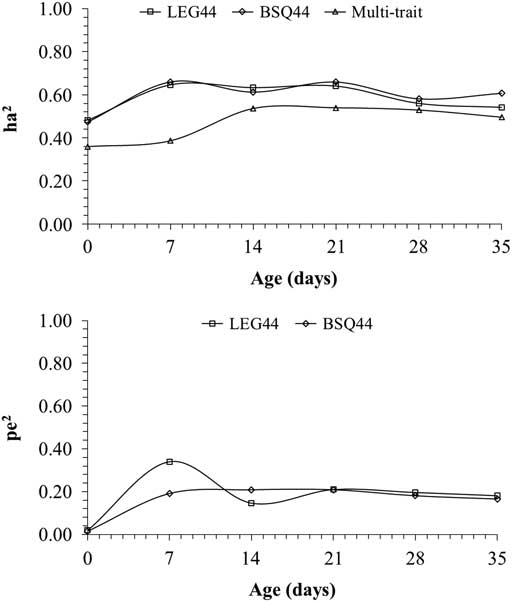
Heritability estimates throughout the growth of quail differed in regards to the RRM using B-spline functions and Legendre polynomials in comparison with multi-trait models (Figure 2). At the beginning of the curve, the estimated heritability for the direct additive genetic effects obtained with residual variance as heterogeneous using RRM with Legendre showed the same trend that those estimated using B-spline functions, but the results obtained from the multi-traits models were lower. Except for the beginning of the evaluation period, the heritability estimates obtained for the direct additive genetic effects showed similarity between the different evaluated models. As a comparison, Resende et al. (Reference Resende, Martins, Georg, Paiva, Conti, Santos, Sakaguti and Murakami2005) reported lesser values of heritability estimates compared with what obtained in the present study (considering multi-trait or RRM); these authors considered multi-trait models with values ranging from 0.33 to 0.48 for BW from hatching until 28 days of age. Gonçalves et al. (Reference Gonçalves, Pires, Pereira, Drumond, Felipe and Pinheiro2012) pointed out that heritability decreased along the growth curve, ranging from 0.51 (day 1) to 0.16 (day 42). As the age increased, heritability estimates decrease as reported by Silva et al. (Reference Silva, Ribeiro, Crispim, Silva, Bonafé, Silva and Torres2013) who evaluated meat-type quail using multi-trait model; these authors obtained values varying from 0.53 at hatching to 0.25 at day 42. Narinç et al. (Reference Narinç, Aksoy and Kaplan2010) reported similar heritability values in Japanese quail for BW at hatching and from 1 to 5 weeks of age. The same group of researchers estimated in another study a heritability value of 0.36 for BW at 35 days in Japanese quail (Narinc et al., Reference Narinc, Aksoy and Karaman2014). Karaman et al. (Reference Karaman, Narinc, Firat and Aksoy2014) reported a lesser heritability estimate for BW at 42 days of age (0.48) than what was found in the present study for BW at 35 days of age. These values were lesser when compared with those estimated by RRM in the present study and greater than the estimated by the multi-trait model.
Direct heritability
 $\left( {h_{a}^{2} } \right)$
and permanent environmental
 $\left( {pe^{2} } \right)$
variance estimates as a proportion of total phenotypic variance obtained with models LEG44 (□), BSQ44 (◊) and by multi-trait analysis (∆). LEG=Legendre polynomial; BSQ=quadratic B-spline functions.

Estimates of permanent environmental variance as a proportion of phenotypic variance showed different behavior for RRM using B-spline functions compared with Legendre polynomials (Figure 2). The permanent environmental variance using Legendre polynomials increased from hatching (0.02) to day 7 (0.34), with a reduction at day 14 and then tended to increase until day 35, exhibiting fluctuations when compared with B-spline functions. The permanent environmental effect in this study increased from hatching (0.01) until day 35 (0.35) indicating that these effects were important at older ages (Figure 2). However, the inclusion of permanent environmental effect contributes for a better distribution of the variance which resulted in more accurate estimates of breeding values. Moreover, the non-inclusion of these effects could overestimate the direct additive variance and consequently the breeding values, resulting in less genetic gain than the expected because of the inaccuracy of the model to estimate the breeding value of quail.
Genetic correlations
The genetic and permanent environmental correlations estimated between BW at hatching until day 35 days using B-spline functions were of medium to high magnitude (Table 4). Genetic correlations decreased with the increase of the distance between BW measurements, and the greatest correlations were obtained at adjacent ages. Genetic correlations above 0.60 suggest that selection for BW can change the adult BW in the same direction. Therefore, adult BW would be subjected to large increases as a result of selection for heavier BW earlier, such as at days 21 and 28. In this manner, these traits could receive greater emphasis on selection index to select quail with heavier BW at a younger age. Our results are consistent with those reported by Bonafé et al. (Reference Bonafé, Torres, Sarmento, Silva, Ribeiro, Teixeira, Silva and Sousa2011), Dionello et al. (Reference Dionello, Correa, Silva, Corrêa and Santos2008) and Gonçalves et al. (Reference Gonçalves, Pires, Pereira, Drumond, Felipe and Pinheiro2012) who reported high genetic correlation from day 7. On the same way, Sezer (Reference Sezer2007) also reported high genetic correlation between not only successive but also early and late weightings and suggested that selection for final BW could be based on early BW measures. The permanent environment correlations were in general similar to genetic correlations. This suggests a strong importance of the permanent effect between the BW from hatching until day 35 and also indicates that permanent environmental factors that affect at younger ages also affect BW at adjacent age.
Estimates of direct additive genetic (below the diagonal) and permanent environment (above the diagonal) correlations between BW from hatching to day 35 obtained from the BSQ44 model. Values within parenthesis are the SD

Genetic trend
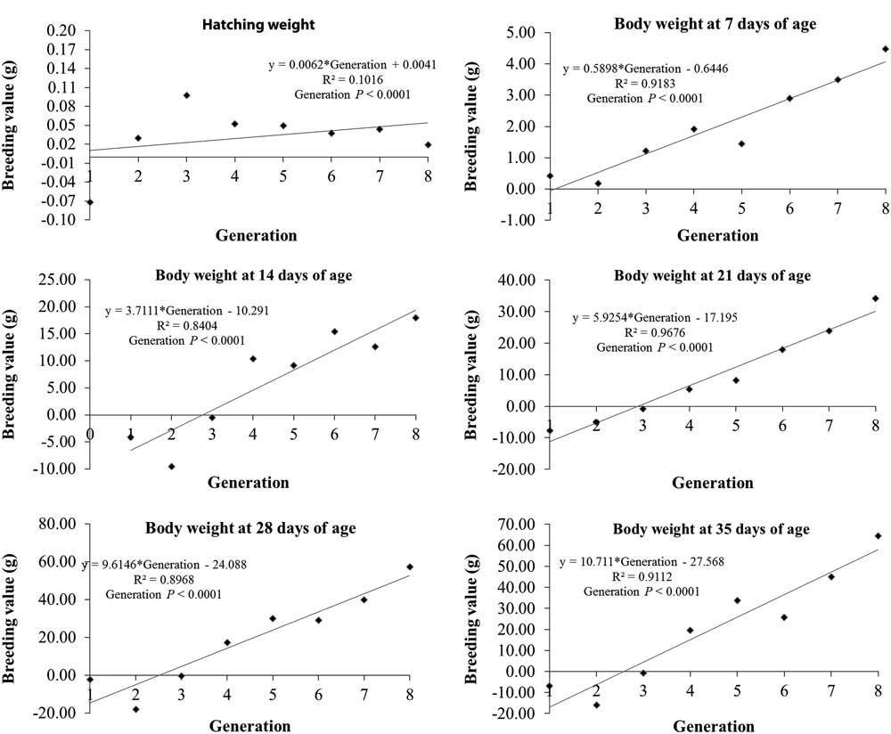
Genetic trend of BW at hatching had low variation among generations, which indicates that quail selection for heavier BW did not affect BW at hatching (Figure 3). Genetic trend of BW measured at days 7, 14, 21, 28 and 35 had a significant linear increase (P<0.001) between the 1 and 8 generations with expected increases of 0.59, 3.71, 5.92, 9.61 and 10.71 g/generation, respectively. In general, genetic trends of quail BW increased over the generations with little fluctuations in some years. The low values for genetic trends between the first and third generations can be explained by the beginning of directional selection for BW. The increase of the breeding value per generation expected from the fourth generation occurred because of the higher selection intensity for BW.
Genetic trend of breeding values for BW at day 0 (hatching), and at days 7, 14, 21, 28 and 35, according to selection generations in meat-type quail.

Selection response
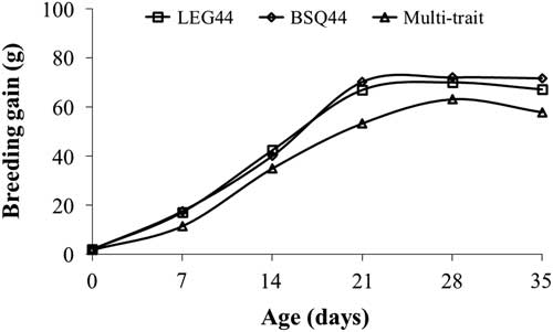
The genetic response to selection for BW in the evaluated ages had greater values for the RRM compared with multi-trait models (Figure 4). These results reflect higher responses to BW selection using RRM. In the same way, the use of B-spline functions and Legendre polynomials showed similar responses until day 28. However, we observed a reduction of genetic response at day 35 when using RRM with Legendre polynomials. This behavior may have been affected by the genetic variance behavior estimated by this model.
Genetic direct gain to BW in meat-type quail estimated by random regression models using functions BSQ44 (◊), LEG44 (□) and multi-trait models (∆). LEG=Legendre polynomial; BSQ=quadratic B-spline functions.

The effect of the genetic gain based on age increased until day 28 proving that there is an effectiveness of selection aimed at BW in the breeding program. There was a tendency of increasing the breeding value of quail for BW at day 28 and this tendency can be attributed to the genetic gain obtained through selection (focused for heavier BW), which is performed at day 28. Thus, the selection response is more pronounced (with great gains intensity) on this trait compared with BW at hatching, although there is a considerable increase in the breeding values of the correlated trait.
In conclusion, RRM using B-spline quadratic function with four residual variance classes and four segments was the one that best adjusted the growth trajectory in meat-type quail. Genetic trends predicted for BW indicated that positive changes are occurring throughout the generations. In addition, the use of B-spline functions provided greatest genetic response for BW selection.
Acknowledgments
The authors thank the Brazilian funding agencies FAPEMIG (‘Fundação de Amparo à Pesquisa do Estado de Minas Gerais’ grant no. BPD 00292-14 - CVZ-PPM 00913-15) and CNPq (‘Conselho Nacional de Desenvolvimento Científico e Tecnológico’; grant no. 474149/2013-7) for financial support, and CAPES (‘Coordenação de Aperfeiçoamento de Pessoal de Nível Superior’) for a fellowship to Lúcio F. M. Mota and Paulo G. M. A. Martins (grant no. 23038.008980/2013-90). In addition, the authors express appreciation to ‘Ajinomoto do Brasil Ind. e Com. de Alimentos Ltda.’, for providing the amino acids utilized in this study, and the UFVJM, Poultry Sector personnel, for the diligent animal care.