


The invention and widespread adoption of wheeled transport for long-distance trade in the form of vehicles pulled by pack animals (wheeled or wagon transport henceforth) is an important technological achievement of antiquity (Piggott Reference Piggott1983; Anthony Reference Anthony2007). However, even by the nineteenth century, despite global diffusion of wagons and access to pack animals through colonization, many places in sub-Saharan Africa or South America had not adopted the wheel (Bulliet Reference Bulliet2016). Slow wheel adoption is even more striking, given its positive economic effects (Dalgaard et al. Reference Dalgaard, Kaarsen, Olsson and Selaya2018; Alvarez-Palau et al. Reference Alvarez-Palau, Bogart, Satchell and Shawn Taylor2025).
Slow adoption of new technology is widespread across time, technologies, and countries (Comin and Hobijn Reference Comin and Hobijn2010). However, the delay in adopting wheeled transport, a well-understood and generally beneficial technology, is remarkable.
Indeed, scholars who have studied slow technology adoption are puzzled. Mokyr (Reference Mokyr1990, p. 161) suggests Amerindians (independently) invented the wheel, but “then turned their attention elsewhere” or “never tried hard” to use the wheel for transportation. Diamond (Reference Diamond1997, p. 359) notes that in Eurasia the wheel was used for land transport, pottery, and clocks, but “none of these uses … was adopted in the [Pre-Columbian] Americas, where wheels are attested only in Mexican ceramic toys.” Further, he suggests that absence of pack animals in the Andes contributed to slow adoption. Yet, this absence cannot explain the almost four-centuries-long delay after Columbus brought pack animals and wheel technology to the continent (Headrick Reference Headrick2012).
We explore this puzzle and propose what is, to our knowledge, the first hypothesis to explain slow adoption of wagon transport over the Andes, even after the arrival of the Spanish. Our explanation emphasizes how incentives, shaped by geography, human and animal physiology, and weak transport demand, influenced adoption timing.
The intuition guiding this hypothesis combines two strands of literature. First, a threshold technology-adoption model (David 1966) is adapted to determine when economic incentives were high enough to induce traffic diversion from a human-porter or animal-pack road to a wagon road. The model’s intuition contrasts a low fixed and high variable cost technology (animal-pack road) with a high fixed and low variable cost technology (wagon road) across production levels (traffic). As the traffic level increases, the high fixed cost of the wagon road is spread over more journeys, and the transport unit cost declines. When wagon transport cost savings (compared to animal-pack transport cost) equate wagon-road construction cost, economic incentives induce its construction, and traffic diverts to it. The level of traffic that makes both costs equal is the traffic threshold.
Second, the model’s variable cost is calibrated using energy transport cost. Since variable transport cost by road is not available, we use archeology and human and equine physiology research (Drennan Reference Drennan1984; Yousef, Dill, and Freeland Reference Yousef, Dill and Freeland1972; Minetti Reference Minetti1995) to calculate human and mule transport energy costs, which vary with slope, as a proxy for variable transport costs. Energy transport cost strengthens the model’s economic intuition and clarifies route choice. As Minetti’s work for humans has highlighted, in mountainous terrain, energy consumption is lower following a straight, steep, short route rather than a zigzagging, gentle, and long route. However, wheeled transport can only be used on zigzagging, gentle, and long routes. Thus, the route choice is different when using human or mule transport compared to when using wheeled transport.
We blend these two strands of literature into a calibrated model to examine the adoption of the first wagon road over the Andes. We use Colombian public works archives to document the first long-distance wagon road. The Cambao wagon road was completed in 1885 and diverted traffic between Bogotá and the Magdalena River from the colonial pack road. These archives allow locating the historical human and animal-pack and wagon routes. Crucially, we can produce detailed slope profiles for both routes. In turn, the slope profiles, complemented by energy transport costs found in secondary literature, and the construction costs found in contemporary project and engineering reports, help to calibrate the threshold technology-adoption model. This follows economic history’s tradition of using a calibrated model to examine an important event (Fogel Reference Fogel1962). This model offers a first step analyzing how incentives shaped this unique observation of wagon-adoption.
The calibrated model allows calculating the wagon-adoption traffic threshold. When the model’s threshold is lower than the observed traffic, incentives were high enough to build the wagon road.
Analysis of the calibrated model suggests that (i) enough transport demand (traffic) existed on the colonial road to make the Cambao wagon road total transport cost lower at some point during the second half of the nineteenth century. This prediction is robust to reasonable changes in parameter values. (ii) The human porter and mule-pack road takes a straight, steep, short route that reduces energy consumption compared to a zigzagging, gentle, and long one, but does not allow for later use of wagons over the same route. Thus, choosing the least-cost route first creates a switching cost. Pre-Columbian and colonial route choices align with energy-saving paths, while the switching costs explain wagon adoption delay. (iii) Counterfactual scenarios suggest that, compared to other mountainous regions, both weak transport demand and geography, as well as human and animal physiology, may have been important factors delaying wagon adoption. Though not an absolute barrier, rugged geography lengthens wagon-route distance relative to a straight-line surface route, increasing location, construction, maintenance, and transport costs.
We also explore complementary explanations. Colombia was a relatively weak state. Incentives to build state capacity likely reinforced wagon construction, while route search costs, the lack of political coordination, and the efficiency of flexible mule-pack train length delayed adoption throughout the 1860s and 1870s.
The paper contributes to our understanding of four issues. First, it clarifies why wagon adoption for long-distance trade was slow and uneven. Bulliet (Reference Bulliet2016) has highlighted cases of slow wheel adoption (South America and Sub-Saharan Africa) and even adoption reversals (the Middle East, North Africa, China, and Japan). We provide the first explanation, to our knowledge, for the long adoption delay in the Andes. It stresses how geography and human and animal physiology affect energy cost and route choice at different transport-demand levels. Transport demand likely surpassed the traffic threshold during the second half of the nineteenth century, following recovery from almost three centuries of demographic collapse after the Spanish arrived in the Americas.
Second, our findings also clarify how geography affects development. Colombian historiography has highlighted the complex, mostly negative developmental effects of the Andes’ breakup and the country’s relatively rugged landscape, even compared to other Andean nations (Safford and Palacios Reference Safford and Palacios2002). Our work suggests that the interaction between topography and human and animal physiology implies that rugged topography lengthens wagon roads, raising adoption cost, influencing contemporaneous agents’ actions to slow development (Gallup, Sachs, and Mellinger Reference Gallup, Sachs and Mellinger1999). Additionally, the breakup also creates river valleys that bring cheap water transport close to many locations, making this breakup both a curse and a blessing (Nunn and Puga Reference Nunn and Puga2012).
Third, switching costs between a human and mule route and a wagon route generate path-dependence (David 1985). Hence, the interaction between geography and human and mule physiology also creates a long-term effect, delaying wagon transport adoption.
Finally, findings also relate to the role of incentives in technology-adoption. Subsidized construction (building ahead of demand) or high transport demand (building following demand) accelerate transport improvements (Fogel Reference Fogel1960; Fishlow Reference Fishlow1965; Harley Reference Harley1980, Reference Harley1982; Mercer Reference Mercer1982; Atack et al. Reference Atack, Bateman, Haines and Margo2010; Duran Reference Duran2013).
THE INVENTION AND GLOBAL ADOPTION OF THE WHEEL
A long-run view of the invention and adoption of wheeled transport provides the global context for our discussion. Wagons first appeared between 4,000 and 3,000 bce in the region surrounding the Black and Caspian Seas. Migration of the Eurasian steppe nomads, the Hittite, Egyptian, and Greek civilizations, and the expansion of the Roman Empire spread the use of wagons throughout the Mediterranean Rim, Northern Europe, and Asia. By 0 CE, only Australia, the Americas, and Sub-Saharan Africa did not use wagons (Piggott Reference Piggott1983; Anthony Reference Anthony2007; Bulliet Reference Bulliet2016).
In Sub-Saharan Africa, wheeled vehicles were used in ceremonies and by the military. Colonization marked the arrival of wagon and rail transport to other activities (Chaves, Engerman, and Robinson Reference Chaves, Engerman and Robinson2013).
In the pre-Columbian Americas, the Olmec used wheels only for decoration and toys (Diamond Reference Diamond1997; Bulliet Reference Bulliet2016). Large pack animals arrived with colonization.Footnote 1
In the United States, use of pack animals and wagons extended with territorial expansion (Taylor Reference Taylor1951). In the Spanish Americas, pre-Columbian human trails were improved to create a mule-pack road network. Wagon use was limited to the pampas, the southern Andean foothills, and, sporadically, to a segment of the Mexico City-Veracruz road. No major road transport advances occurred before the mid-nineteenth century (Duran, Páez, and Torres Reference Duran, Páez and Torres2020).
At the mid-nineteenth century, interest in overland transport grew in Latin America, and short railways off the Andes were built. The first Andean wagon road was completed in Colombia in 1885, while rails supported Peruvian Andean mining in the 1870s (Duran, Páez, and Torres Reference Duran, Páez and Torres2020).
TRANSPORT BETWEEN BOGOTÁ AND THE MAGDALENA RIVERFootnote 2
At the end of the nineteenth century, Colombia was a poor and isolated country located in the northwestern corner of South America. As the Andes arrives in southern Colombia, it breaks into three branches heading north, creating a rugged landscape. The Magdalena River runs through a valley between the eastern and the central mountain ranges, discharging into the Caribbean Sea. It is the most important waterway in Colombia.
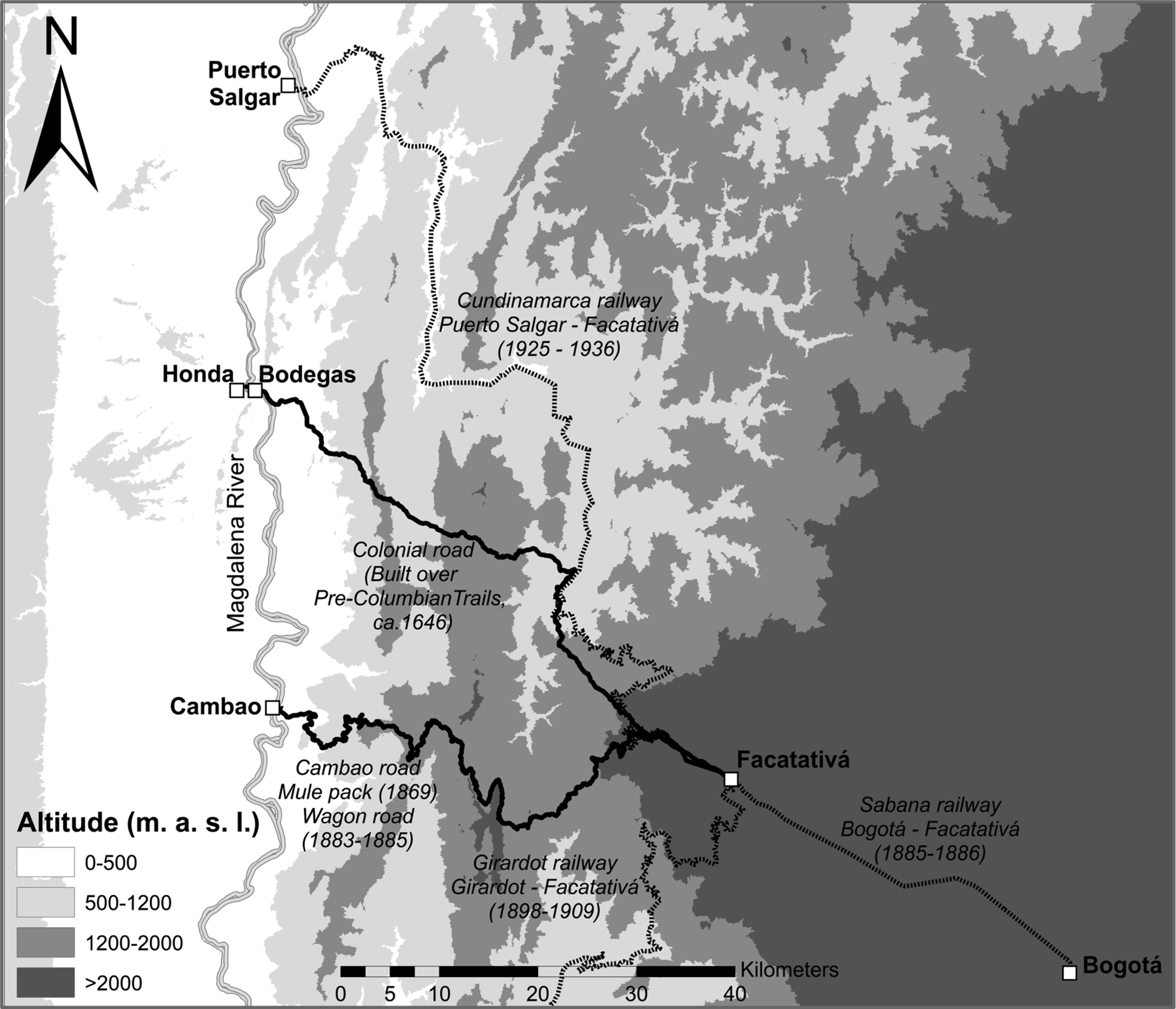
Bogotá, Colombia’s most populous city and political capital since colonial times, sits atop the eastern range in a flat, large, and fertile area called sabana, 2,600 meters above sea level (MASL). In colonial times, a 127-kilometer mule-pack road (colonial road henceforth), built over pre-Columbian paths in the sixteenth century by the Spanish Crown, connected Bogotá to the Magdalena River (see Figure 1). It connected Bogotá to Facatativá, on the sabana’s western border. The road descended, crossing two ranges to reach the Magdalena River at Bodegas, at just over 200 MASL. The trip took four to six days by porter or mule. The road connected settlements that served transporters and travelers. Maintenance followed European custom: communal work and state toll-funded tools. In the 1800s, a state committee oversaw toll collection and road maintenance. The road was Bogotá’s sole external connection (Codazzi Reference Codazzi2003).
MAP OF BOGOTÁ’S SABANA, MULE-PACK, WAGON, AND RAILWAY ROUTES TO THE MAGDALENA RIVER
Note: Road construction dates in parentheses.
Source: Own construction.

Colombia changed in the 1850s. The Liberal Party dominance pushed for economic liberalism. The following decades saw sporadic tropical product export booms and a sustained coffee export boom. These booms fueled transport improvement proposals (Safford and Palacios Reference Safford and Palacios2002).
The late 1850s and 1860s saw three wagon road proposals emerge, linking Bogotá to the Magdalena. All routes met in Facatativá but varied in the descent path. Camacho (Reference Camacho1858), future Secretary of Finance, proposed a wagon road in 1858 to Girardot to transport Bogotá’s growing international trade and regional agricultural exchange. In the 1860s, Indalecio Liévano, professor at the Engineering School of the National University and director of the National Astronomic Observatory, surveyed potential routes. In 1863, he reported the Girardot route inadequate for wagons. In 1865, he favored a route to Honda. In 1869, a route proposed by the Chorographic Commission, linking Facatativá to Cambao (continuing to Bodegas on steamers), was found to be the best. It crossed sparsely inhabited territories, with good food and water supply, arriving close to the rising tobacco-exporting city of Ambalema (Lievano Reference Lievano1865; Pereira Reference Pereira1870).
Initially, in 1869, the colonial road administration committee built a one-meter-wide mule-pack road over the wagon route at $31,200 (all monetary values are expressed in 1858 pesos) to test feasibility and estimate the likely cost of expanding it into a wagon road. The plan was to expand the pack road into a six-meter-wide wagon road in three years at a total cost of over $312,000 pesos (Lievano Reference Lievano1865; Pereira Reference Pereira1870).
The wagon’s road route location was now clear. However, public interest was moving to building a railway. In 1865, transport policies promoted wagon and rail transport equally. By 1872, only rail could receive federal government subsidies. In 1874, the Cundinamarca state granted a concession contract to the Occidental Railway Co., a private company, to link Bogotá and Bodegas. The contract included building from east to west and west to east to increase construction speed; hence, the company was responsible for expanding the Cambao mule-pack road into a wagon road on which to take rail inputs into the sabana prior to rail line completion. By the late 1870s, the works stalled amid corruption allegations; the dream of rail transport to the Magdalena faded into disillusion (Corredor and Nieto Reference Corredor and Nieto1880; Lézmes et al. Reference Lézmes, Restrepo, Gutiérrez and Espinosa1883).
In 1882, the original concession contract was renegotiated and divided into two separate railway lines and companies. The Occidental Railway Co. was to build and operate under a concession contract the line between Bodegas and Facatativá. Cundinamarca’s government was to own, build, and operate the rail line connecting Facatativá to Bogotá, the Sabana Railway Co (Lézmes et al. Reference Lézmes, Restrepo, Gutiérrez and Espinosa1883).
In practice, renegotiation was more of a legal solution to allocate construction of the Bogotá-Facatativá railway to the government than to reinvigorate construction of the Magdalena River-Facatativá railway. At the time, low expected profitability and transition to centralism in 1886 stalled the mountain railway. Legal conflicts, contractual changes, and corruption allegations delayed construction into the late 1920s, and the railway was completed in 1936 (Pérez 2008).
Once the Sabana Railway Co. was organized in 1882, Cundinamarca formed a commission to advise on how to organize rail-line construction between Bogotá and Facatativá. Due to fiscal limits and no rail link from the river, the commission recommended extending the Cambao mule-pack path into a scaled-down wagon road to transport railway inputs into Bogotá’s sabana. The path would be widened into a one-way three-meter-wide road (instead of the two-way six-meter-wide road originally planned) with key two-way sections to allow for two-way traffic. The wagon road was completed in 1883–1885 at $69,690 pesos and opened to traffic on 8 August 1885. The wheel arrived in the Andes for long-distance trade before the short and relatively flat Barranquilla, Cúcuta, and Sabana railways were completed in the late 1880s (Nieto and Aldana Reference Nieto and Aldana1885).
The Cambao wagon road was used to transport the Sabana Railway Co. inputs. Bogotá’s entrepreneurs took advantage of the new transport and brought inputs for the first modern electricity-generation plant, aqueduct, municipal theater, and beer factory, among many initiatives. Bogotá began its modern industrialization (Duran, Páez, and Torres Reference Duran, Páez and Torres2020).
A THRESHOLD TECHNOLOGY-ADOPTION MODEL OF WAGON TRANSPORT
The construction of the Cambao wagon road in 1885 marked the arrival of the wheel in the Andes. In this section, we develop a threshold technology-adoption model (David 1966) adapted to wagon transport in the Andes to examine incentives for its construction.
Wagon transport is adopted when it costs less than mule-pack. Initially, a low fixed-cost and high variable-cost technology (mule-pack) exists. The colonial mule-pack road followed a straight, steep, short route to reduce construction and maintenance costs by minimizing the road’s distance and the use of bridges, tunnels, or earth movements required. With construction sunk, total annual mule-pack cost is given by road maintenance cost, M m , and the transport cost, mq, with m being the average mule transport price per ton-roundtrip and q traffic in tons. An alternative high fixed-cost and low variable-cost technology (wagon road) also exists. The wagon road follows a more zigzagging, gentler, longer route that requires a longer distance and more substantial earth movements, making it more expensive to build and maintain. However, it allows for the use of wagons that reduce unit transport cost. Total annual cost over the wagon road is a fixed (one-off) entry construction cost, C, plus the road maintenance cost, M w , and the transport cost, wq, with w as the average wagon transport price per ton-roundtrip. As transport demand (traffic) grows with, for instance, increasing population or regional long-run development, the fixed construction and maintenance cost of the wagon road spreads over a higher number of units of traffic, and the unit cost declines. Thus, wagon transport is adopted when total annual mule-pack cost is higher than that over the wagon, and the adoption condition is defined by

The adoption-threshold traffic level is the traffic level that makes total wagon cost equal to that of the mule-pack and is given by

The threshold traffic level induces construction of the wagon road and diversion of through traffic from mule-packs to wagon transport. Since transport projects are frequently built and operated over multiple time periods, the problem of choosing the threshold traffic level becomes intertemporal and requires the use of a discounted cash-flow set-up. The project intertemporal adoption-threshold traffic level includes the financial cost to pay for road construction over several periods (taxes or debt), r i , and the social preference to consume today compared to tomorrow (social discount rate), r s , and is given by

The model calibration uses the observed ex-post average maintenance cost per kilometer for each road, the average construction cost per kilometer for the wagon road, and mule and wagon road distance to calculate total construction and maintenance costs.
The average mule-pack road and wagon road costs are not available. The energy cost of transport—the cost of the foodstuff necessary to supply the energy consumed by humans and animals when performing transport work—provides a reasonable, even if rough, approximation.
The mule and wagon transport average cost per ton-trip, m and w, varies depending on the length and the slope profile of the road. Longer or steeper roads increase a mule’s energy consumption cost per ton-trip. On mountainous landscape, between any two origin and destination locations, a wagon road is gentler but also longer than a mule-pack road. Thus, the energy consumption net effect of a gentler slope but longer road is ambiguous.
Average mule transport cost per ton-roundtrip, m, is defined by the annual average energy cost of mule transport operating at its maximum capacity throughout the year. Thus, a mule’s annual energy consumption, E m , divided by the energy generated by one kilogram of foodstuff, k, gives the number of kilograms of foodstuff necessary to perform transport work per annum. In turn, the quantity of foodstuff multiplied by its price per kilogram, p, gives the annual energy cost of transport. Annual fixed operation cost is O m , including driver (labor, food, and lodging) and mule (acquisition and depreciation) costs. Annual energy and fixed operation costs are then divided by the kilograms weight of load carried, L m , and the number of annual roundtrips, RT m , times 1,000 to calculate the mule transport annual average cost per ton-roundtrip, as described by Equation (4).

The wagon average cost per ton-roundtrip, w, is defined analogously. The annual energy consumption term is identical. We assume equal energy consumption, whether mules carry loads or pull wagons; mule effort is exerted at a high level in both transport modes. We also assume mules carry and pull loads in line with historical contemporary evidence (see Appendix Table 1). The O w term includes the annual driver’s and mules’ cost, plus wagon (acquisition and depreciation) cost, and the river section cost (shipment and transshipment per ton cost for all tons transported).
In turn, annual energy consumption, E m , is defined in Equation (5) as the mule and load weight, (B m + L m ), multiplied by roundtrips, RT m , and multiplied by energy consumption per roundtrip and kilogram of weight, (•). In turn, energy consumption per roundtrip is the summation of energy consumption at kilometer d and slope i per minute, e di , times the number of minutes it takes to travel over that one kilometer at slope i and speed s dim , 60/s dim . The total energy consumed on the wagon road is defined analogously.

Next, travel speed at kilometer d at slope i,  , is defined as a speed between the minimum and the maximum speed that is proportional to the energy consumption at kilometer d at slope i relative to a kilometer at maximum slope on the colonial mule road, as in Equation (6).

Finally, the annual number of roundtrips, RT m , is defined by Equation (7) as N working days divided by the number of days it takes to perform a roundtrip on the colonial mule road, that is, the summation of minutes it takes to travel over a kilometer d at slope i divided by 480 minutes per working day of eight hours.

Replacing Equations (4), (5), (6), and (7) into Equation (2), simplifying and transforming into implicit functions, the equilibrium threshold traffic triggering adoption of the wagon road is given by Equation (8).Footnote 3

The larger the fixed construction cost or difference between the wagon and mule annual road-maintenance cost, the higher the threshold traffic level. Since construction of the colonial and wagon road involved no tunnels, bridges, or major earth movements, construction and maintenance costs depend on total road distance. Thus, the longer the distance of the wagon road compared to that of the colonial road, the higher the traffic threshold to induce wagon road adoption.
The lower the wagon average per ton-roundtrip cost compared to that of the mule (on the colonial road), the higher the cost advantage of wagon transport and the lower the traffic threshold. In turn, the lower the slope and distance of the wagon road, the smaller the energy consumption and travel time, and the higher the cost advantage of the wagon road.
The threshold technology-adoption model adapted this way enables us to (i) study the role of incentives on the adoption of the wheel in the Andes and (ii) infer the timing of adoption by comparing threshold and observed traffic levels. It allows for the possibility that even if knowledge about such a revolutionary invention as the wheel had already spread throughout the world, it may not have been efficient to adopt the wheel in some parts of the world, like the Andes. Furthermore, adoption may reverse if transport demand declines.
MODEL CALIBRATION USING CONTEMPORARY INFORMATION AND RESULTS
We calibrate the threshold technology-adoption model using contemporaries’ intuition and information to anchor it as accurately as possible to the historical context. This section develops a first approximation, using the project reports to calibrate the model’s Equation (2). In the next section, we also use energy consumption and route slope profile information to calibrate Equations (4), (5), (6), and (7).
The thought experiment performed by the calibrated model to identify the threshold traffic is described by Equation (2), as follows. In 1858, a social planner (government) transport supplier hires a driver and buys a two-draft-animal team. She pays the driver a daily wage, including food and shelter. She pays the annual rent equivalent of buying a two-draft-animal team using a loan, depreciated over two years.Footnote 4 If she decides to offer wagon transport, she builds the road and receives transport savings instantaneously. She pays the fixed (one-off) entry construction cost (C) using tax revenue and the annual rent equivalent of buying a cart, depreciated over five years.
Next, she compares the transport cost of a driver on the colonial road walking a two-draft-animal team against the transport cost of a driver on the Cambao road walking a two-draft-animal team pulling a cart.Footnote 5 If the transport cost of wagon transport is lower than that of mule-pack, she compares the transport cost savings (produced by all roundtrips per annum) to the wagon-road construction cost, and the net wagon-mule roads maintenance costs and computes the traffic threshold. If the threshold is lower than traffic observed on the colonial road, incentives are high enough to build the wagon road. If not, the social planner waits until colonial road traffic increases enough to justify construction. Appendix Table 1 shows parameter values and sources, mostly contemporary entrepreneur and engineering reports, that anchor the model to the historical context.Footnote 6
The calibrated model predicted that mule-pack freight on the colonial road (excluding unobserved transport supplier profits) is about 70 percent of observed contemporary freight (Online Appendix OA1). Thus, the model provides a reasonable out-of-sample fit.
Analysis Using the Model Calibrated with Contemporary Information
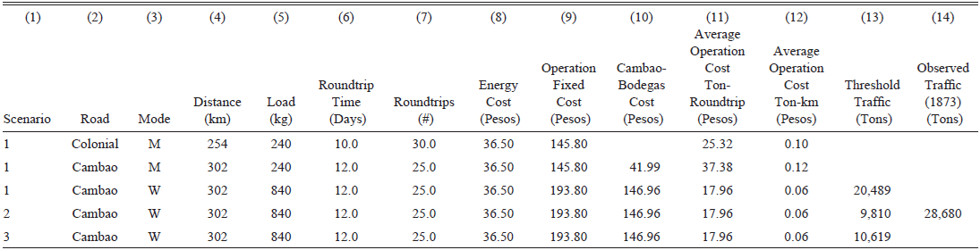
The baseline results are presented in Table 1. It shows that a two-animal pack on the colonial road covers the 254-kilometer-long roundtrip transporting a 240-kilogram load in ten days and performing 30 roundtrips per annum. A driver earns $0.30 pesos daily (300 days per annum), while the team annual cost is $55.80. The driver and team represent operational fixed costs that add up to $145.80 per annum. Animal feed is $0.05 per night, making annual energy cost $36.50. The average operational cost per ton-roundtrip using animal-pack transport on the colonial road is $25.32. See details in Duran and Guerra-España (2026).
MULE-PACK AND WAGON FREIGHT ROUNDTRIP COST OVER COLONIAL AND CAMBAO ROADS AND TRAFFIC THRESHOLD, MODEL CALIBRATED USING CONTEMPORARY INFORMATION

Table 1 Long description
A table comparing freight roundtrip costs over colonial and Cambao roads and traffic thresholds. The table has 14 columns and 4 rows, including a header row. The columns are labeled as follows: (1) Scenario, (2) Road, (3) Mode, (4) Distance (km), (5) Load (kg), (6) Roundtrip Time (Days), (7) Roundtrips (#), (8) Energy Cost (Pesos), (9) Operation Fixed Cost (Pesos), (10) Cambao-Bodegas Cost (Pesos), (11) Average Operation Cost Ton-Roundtrip (Pesos), (12) Average Operation Cost Ton-km (Pesos), (13) Threshold Traffic (Tons), (14) Observed Traffic (1873) (Tons). Row 1: Scenario 1, Colonial, M, 254, 240, 10.0, 30.0, 36.50, 145.80, 145.80, 25.32, 0.10, 20.489. Row 2: Scenario 1, Cambao, M, 302, 240, 12.0, 25.0, 36.50, 145.80, 41.99, 37.38, 0.12, 28.680. Row 3: Scenario 1, Cambao, W, 302, 840, 12.0, 25.0, 36.50, 193.80, 146.96, 17.96, 0.06, 9.810. Row 4: Scenario 2, Cambao, W, 302, 840, 12.0, 25.0, 36.50, 193.80, 146.96, 17.96, 0.06, 10.619.
Notes: Scenario: Threshold traffic is calculated under three different scenarios. Scenario 1 assumes the project’s costs and benefits occur instantaneously in year 1, as in Equation (2). Scenario 2 assumes the project’s construction cost is invested in year 0 and financed with taxes at zero opportunity cost; maintenance costs and transport cost savings occur during the following five years, following Equation (3). Scenario 3 assumes the project’s construction cost is invested in year 0 and financed with an international bond issue at a yield of 7 percent per annum; maintenance costs and transport cost savings occur during the following five years, following Equation (3). Road: Colonial and Cambao. Mode: Transport mode used; mule-pack (M) or wagon (W). Distance: Roundtrip distance of the road. Load: Load in kilograms carried by mule-pack or wagon. Roundtrip time: Number of days to complete roundtrip journey. Roundtrips: Number of roundtrips per annum. Energy cost: Cost of feeding mules in pesos per annum. Operation fixed cost: Cost of driver, mules (including purchase, depreciation, and finance cost), and wagon in pesos per annum. Cambao-Bodegas cost: Cambao-Bodegas steamer roundtrip transport cost plus transshipment into wagon cost in pesos per annum. Average operation cost pesos ton-roundtrip: ((7) + (8) + (9))/(6)/(4) * 1,000. Average operation cost pesos ton-km: ((7) + (8) + (9))/((6) * (3))/(4) * 1,000. Threshold traffic: Traffic that makes transport cost savings equal construction cost minus net maintenance cost. Observed traffic: Traffic observed over colonial road in 1873.
Source: Own calculations.
When comparing the cost of using the two-mule-pack over the colonial and Cambao roads, it is necessary to consider the latter’s longer road distance (302 km) and roundtrip time (12 days), as well as the steamer Bodegas-Cambao section at $41.99, all making the cost of animal-pack transport per ton-roundtrip $37.38. Hence, Cambao offers no transport cost advantage for animal-pack transport.
However, if a wagon is used, the operation’s fixed cost increases to $193.80 and the load capacity to 840 kilograms, reducing average operation cost per ton-roundtrip to $17.96; using a wagon over Cambao offers lower transport costs. Transport cost savings derive from lower per ton-kilometer cost that declines from $0.10 to $0.06. Transport cost savings are enough to compensate for Cambao’s construction cost when traffic (threshold) reaches 20,489 tons per annum.
Note that this traffic threshold assumes a stringent project baseline setup in which the road is built instantaneously, and the stream of benefits arrives within the first year (Scenario 1 in Column (1), Table 1). Equation (3) relaxes this setup and allows a longer period to finance road construction and enjoy benefits. We assume two contrasting scenarios. In scenario 2, construction takes one year, during which no transportation occurs, t=0. Construction cost is financed with taxes at 0 opportunity cost. The stream of maintenance costs and transport cost savings occurs between years 1 and 5, the typical contemporary horizon. Although Camacho did not explicitly use a discount rate, contemporary infrastructure and mining entrepreneurs did. We assume a low social discount rate of 3.5 percent (Judah Reference Judah1854; Brackenborough, McLean, and Olroyd Reference Brackenborough, McLean and Olroyd2001; Groom et al. Reference Groom, Drupp, Freeman and Nesje2022). In this scenario, the threshold declines to 9,810 tons per annum.
In scenario 3, construction takes one year and is financed using an international bond issue at a 7 percent yield per annum, the typical railway bond yield at the time, and it is paid back between years t = 1 and t = 5. The stream of net maintenance costs and transport cost savings flows between years t = 1 and t = 5. In this scenario, the threshold is 10,619 tons per annum. Overall, the threshold traffic level declines from roughly 20,000 tons per annum in the instantaneous setup to 9,000–10,000 tons in the more flexible setup.
A colonial road traffic series is not available; hence, we take a three-pronged approach to get a sense of transport demand. First, we examine the traffic observations available. Next, since transport demand is derived from aggregate economic activity, which, in turn, depends (partially) on population size, we also examine population trends. Further, we examine the changing transport demand.
In 1869 and 1873, the colonial road administration published estimated total traffic of 16,857 and 28,680 tons per annum, respectively (Pinzon Reference Pinzon1880). Note that traffic level difference between 1869 and 1873 is substantial. Since no other traffic data is available, it is difficult to ascertain the accuracy of these two observations. We use them at face value to exemplify interpretation of the calibrated model results but focus more on their growing trend than on the speed implied.
If we assume the instantaneous project setup (scenario 1) and take colonial-road traffic estimates at face value, by 1873, observed traffic had surpassed the 20,489-ton traffic threshold, inducing wagon road construction. If we assume the more flexible project scenarios 2 and 3, the 9,000–10,000-ton traffic threshold had likely been exceeded before 1869, but we cannot indicate precisely when.
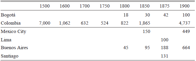
We can attempt to explore further approximately when incentives to adopt wagon transport were high enough to induce construction, as suggested by the calibrated model. Since transport demand is derived from aggregate economic activity, population trends may help to roughly identify the timing when colonial road traffic surpassed the model’s traffic threshold. In 1793, Bogotá’s population was approximately 18,000 inhabitants; in 1851, it was 30,000, and in 1905, it was 100,000 (see Table 2). Early nineteenth century saw slower population growth, while the second half of the nineteenth century saw much faster population growth. If we assume that traffic grew somewhat proportionally to population, traffic was about 12,000 tons in 1851 and 7,000 tons in 1793; the threshold could have been surpassed by the end of the first half of the nineteenth century.
POPULATION OF COLOMBIA AND LATIN AMERICAN CAPITALS, 1500–1900 (1,000S INHABITANTS)

Table 2 Long description
A table comparing population growth in Colombia and Latin American capitals from 1500 to 1900. The table has 6 rows and 9 columns. The columns are labeled with years: 1500, 1600, 1700, 1750, 1800, 1850, 1875, and 1900. The rows are labeled with locations: Bogotá, Colombia, Mexico City, Lima, Buenos Aires, and Santiago. Row 1: Bogotá, 1500, no value; 1600, no value; 1700, no value; 1750, no value; 1800, 18; 1850, 30; 1875, 42; 1900, 100. Row 2: Colombia, 1500, 7000; 1600, 1062; 1700, 632; 1750, 524; 1800, 822; 1850, 1865; 1875, no value; 1900, 4737. Row 3: Mexico City, 1500, no value; 1600, no value; 1700, no value; 1750, no value; 1800, 150; 1850, no value; 1875, no value; 1900, 449. Row 4: Lima, 1500, no value; 1600, no value; 1700, no value; 1750, no value; 1800, 100; 1850, no value; 1875, no value; 1900, no value. Row 5: Buenos Aires, 1500, no value; 1600, no value; 1700, no value; 1750, no value; 1800, 45; 1850, 95; 1875, 188; 1900, 664. Row 6: Santiago, 1500, no value; 1600, no value; 1700, no value; 1750, no value; 1800, no value; 1850, no value; 1875, no value; 1900, 131.
Sources: Bogotá: 1793 (Duran and Diaz 2012 (1794), p. 11), 1851, 1870, 1905 (Florez and Romero 2010, p. 410); Colombia: 1500–1750 (Tovar Reference Tovar2015), 1800–1900 (Florez and Romero 2010); Mexico City: 1859 (Instituto Nacional de Estadística 2009, p. 128); Buenos Aires: 1810, 1850 (Dirección General de Estadística y Censos 2010, p. 128); Mexico City, Lima, Buenos Aires, Santiago 1875, 1900: (Scobie Reference Scobie1986, p. 209).
Long-term and cross-city population trends also help to understand the big picture. Data on Bogotá’s long-term population is not available, but it is available for Colombia. If we assume that Bogotá’s population trends roughly mimic those of Colombia, once the Spanish conquest began, population declined dramatically until 1750, when the territory that is today Colombia was inhabited by about half a million people. As aggregate economic activity likely declined as population fell, incentives to adopt wheeled transport declined. Population growth after 1750 would have increased the incentive to adopt wagon transport, particularly during the second half of the nineteenth century when population more than doubled.
Cross-city population trends suggest that Bogotá was a relatively small place compared to other Latin American capitals. For instance, Bogotá was consistently smaller throughout the nineteenth century than Buenos Aires, Mexico City, Lima, or Santiago. Thus, aggregate economic activity and incentives to adopt the wheel in Bogotá were smaller than those of other capitals outside the Andes.
A complementary argument suggesting that incentives to adopt wagon transport in Bogotá increased during the second half of the nineteenth century lies in the changing nature of traffic. The threshold model does not consider quality-adjusted transport costs. Until the mid-nineteenth century, traffic on the colonial road was probably of a similar nature to that of the past three centuries. As Europe and the United States industrialized during the first half of the nineteenth century, modern machinery became available for other regions to adopt. Indeed, an important motivation for building the Cambao wagon road was to transport railway inputs, and it transported other modern industrial technologies into Bogotá. For instance, before the Cambao road opened, a few railway rails (120 kilograms and six meters long) were transported at $56 per rail over the colonial road, whereas, once wagon transport opened, rails were transported at $8 a piece (Nieto and Aldana Reference Nieto and Aldana1885). Thus, once high-fixed-cost machinery became available and Bogotá’s growth induced its adoption, the increased transport quality (weight and volume) offered by a wagon implied a quality-adjusted transport cost that was lower than its nominal cost. Contemporaries were aware of this difference.
In short, the analysis of traffic, population, and trade information highlights the importance of transport demand in explaining the timing of adoption of wheeled transport for communication between Bogotá and the Magdalena River during the second half of the nineteenth century. Demographic collapse explains low transport demand for almost four centuries following the Spanish arrival. Demographic recovery and increasing trade of larger, heavier industrial capital goods as the nineteenth century progressed suggest that transport demand increased substantially and played an important role in inducing wagon adoption.
We also explore these baseline results by performing a sensitivity analysis. We vary the value of each parameter and consider the situation where the road could have been built ahead of demand. We find that the baseline scenario is qualitatively robust. However, two caveats exist. First, the framework setup overlooks unobserved route search and political costs. Second, given 1873 demand, the cost of a fully two-lane-wide and good-quality wagon road was out of the scope of economic incentives at the time (see Online Appendix OA2).
Even if we have shown that transport demand likely played a key role determining the timing of wagon transport adoption, explanations of historic events tend to be complex and involve many factors. A complementary explanation for inducing wagon transport adoption is that Cundinamarca’s government could have invested to increase its capacity. State capacity is a state’s ability to collect taxes (fiscal capacity) and enforce the law (administrative capacity) (Besley and Persson Reference Besley and Persson2009).
A view prevails that in the Spanish Latin American colonies, state capacity was relatively low and persisted over the nineteenth century (Grafe and Irigoin Reference Grafe and Irigoin2012). The Cambao wagon road’s construction cost was high relative to Cundinamarca’s tax income (32 percent in 1870, while the full two-lane-wide wagon road cost was equivalent to 100 percent) while the state (and country) had no access to the international capital market after it defaulted on its independence debt.
Even if state capacity was low at the time, it is possible that incentives to increase it existed and that a wagon road contributed to its growth. Indeed, transport improvements can help increase tax revenue and closely monitor state agents, enhancing state capacity (Bignon, Esteves, and Herranz-Loncán 2015; Mastrorocco and Teso Reference Mastrorocco and Teso2023). Although it is difficult to assess motivations in collective projects, the first project to build a wagon road (Camacho Reference Camacho1858) mentioned that transport improvements increased “cohesion in customs, institutions and civilization between different peoples of the human family … [and] … building strong conservative interests for public peace” (p. 12). Furthermore, once the completed wagon road and rail line transported goods, it likely helped to increase economic activity and tax revenue. Even if it is not clear when incentives to build state capacity increased, evidence suggests that contemporaries considered the advantages of transport improvements in building state capacity and that some of these advantages likely materialized.
On the other hand, adoption was delayed for about two decades due to route uncertainty, political conflict, and railway optimism. The 1869 wagon-road route took a decade to be located after Camacho proposed the first project. Simultaneously, as different regions competed over where to search for and build the road, legislation to build a wagon road may have been delayed. After the Cambao road route was located in 1869, the legislature preferred to push forward a railway project. In 1882, after realizing that a rail line to the Magdalena would take decades to complete, the legislature promoted a wagon road to build the Sabana railway (Duran, Páez, and Torres Reference Duran, Páez and Torres2020).
Another factor likely delaying wagon adoption was the efficiency of longer mule-pack trains. Contemporary reports simplified the framing of the wagon road investment decision by abstracting the possibility of using longer mule-pack trains. While the driver cost remains fixed, one driver can guide one or many animals. Colombian sources lack historical details on the frequency distribution of train size or the effect of train size on mule-pack transport prices, but one case mentions use of ten animals per driver (Ferro Reference Ferro1994). The calibrated model shows that as the animal train size increases, mule-pack transport becomes more competitive, increasing the threshold traffic level and delaying adoption of the wheel. As mule-pack train size increases from two to three animals, the threshold increases by about 50 percent and continues to rise with train size in marginally declining increments. However, also note that since driver and wagon costs are fixed, wagon transport may also exhibit scale economies as the mule team and wagon capacity increase. Thus, the mule-pack transport advantage derived from increasing mule train may be (at least partially) counterbalanced by initiating wagon transport at a higher scale.
In sum, weak transport demand from 1500–1850 likely played a key role in delaying the adoption of wheeled transport in the Andes, while growing transport demand during the second half of the nineteenth century contributed to its adoption. Incentives to build state capacity likely also induced adoption, while the flexibility of the mule-pack train size, uncertainty about the location of the wagon route, interregional political rivalries, and unwarranted optimism about rival rail-transport adoption delayed wagon adoption.
MODEL CALIBRATION USING TRANSPORT ENERGY COST AND RESULTS
The model calibrated using contemporary information suggests that growing transport demand after the mid-nineteenth century likely played a key role in inducing the adoption of wheeled transport at the end of the century. However, the calibrated model, as it is, does not explain why mule-pack transport was efficient for such a long period of time—almost four centuries—other than wheel transport facing the difficulties of a low-traffic setting in the Colombian Andes. In this section, we enhance our model by incorporating variable transport energy costs based on the road’s slope profile, using the model’s Equations (4) to (7). This will help us better understand the role played by Andean geography in the decision to build a wagon road.
Transport energy cost is measured as the cost of food necessary to supply energy for humans or animals to perform transport work, whether walking, carrying a load on their back, or pulling a wagon. In turn, to identify this cost, we need to estimate energy requirements for transport (henceforth E) and energy supply from nutrients embodied in food.
E includes maintenance and exercise energy. Maintenance E involves the energy needed to maintain stable body weight and support of non-active functions like sleeping or resting; it is typically estimated based on the subject’s weight (even though body composition, gender, age, breed, temperament, and climate may affect actual requirements). Exercise E includes the additional metabolism required for generation of muscular force adjusted by the efficiency of converting metabolic energy into useful mechanical work and heat; it is commonly estimated as a multiple of maintenance E. Experiments based on the rate of oxygen consumption estimate E, measured as milliliters of O2 (VO2) (although exercise at aerobic capacity accumulates lactate that uses energy but would not be reflected in estimates based purely on oxygen consumption figures). In turn, VO2 is multiplied by a coefficient to calculate E in Joules (J) (Harris Reference Harris1997).
The energy required to perform physical activity by humans and animals is supplied by nutrients embodied in food. In turn, the energy potential of food may be conceptualized in different ways. We use digestible energy or metabolizable energy; one digestible energy megajoule (MJ) supplies one energy requirement MJ. The digestible energy content of a ration of a given foodstuff may be estimated in vivo and provides a practical guide; animal nutrition textbooks provide tables indicating the digestible energy in MJ per kilogram for different foodstuffs (McDonald et al. 2011).
Next, we calculate E for a roundtrip over the colonial and wagon roads for humans and mules. We use the slopes of both roads and the E for humans and mules by road kilometer at slope i.
Each route slope profile was produced based on fieldwork. First, the historical routes were identified. The colonial road remains visible, though it is harder to trace through modern settlements. Street names and locations with respect to the historic central square were used to infer the most likely route. The road’s location was mapped by walking it and geolocating its position using GPS. The road, as identified, measures 84.6 kilometers between Bodegas and Facatativá, compared to travelers’ historical records that state a length of 88 kilometers (Codazzi Reference Codazzi2003).
The Cambao nineteenth-century wagon road required a more elaborate approach to locate it. The historic construction reports available do not provide detailed information on the road’s location, and the original road is now part of an extensive network of tertiary dirt roads. Thus, its location was inferred using the information included in the construction reports and identifying key locations, such as settlements or geographical references like rivers, mountain-pass crossings, large rocks, or landscape views. The comparison of these key locations against early twentieth-century maps of the road, air photography that revealed some vestiges of the original road that had been realigned more recently, and the road’s current network all aided in the identification of the historic Cambao road route during visits to the region. Once the road had been located, the route’s coordinates were collected while walking and driving on the road and using GPS and Google Maps. The road, as identified, measures 105 kilometers between Cambao and Facatativá, while the road’s construction report, when it opened in 1885, states a length of 112 kilometers (Nieto and Aldana Reference Nieto and Aldana1885).
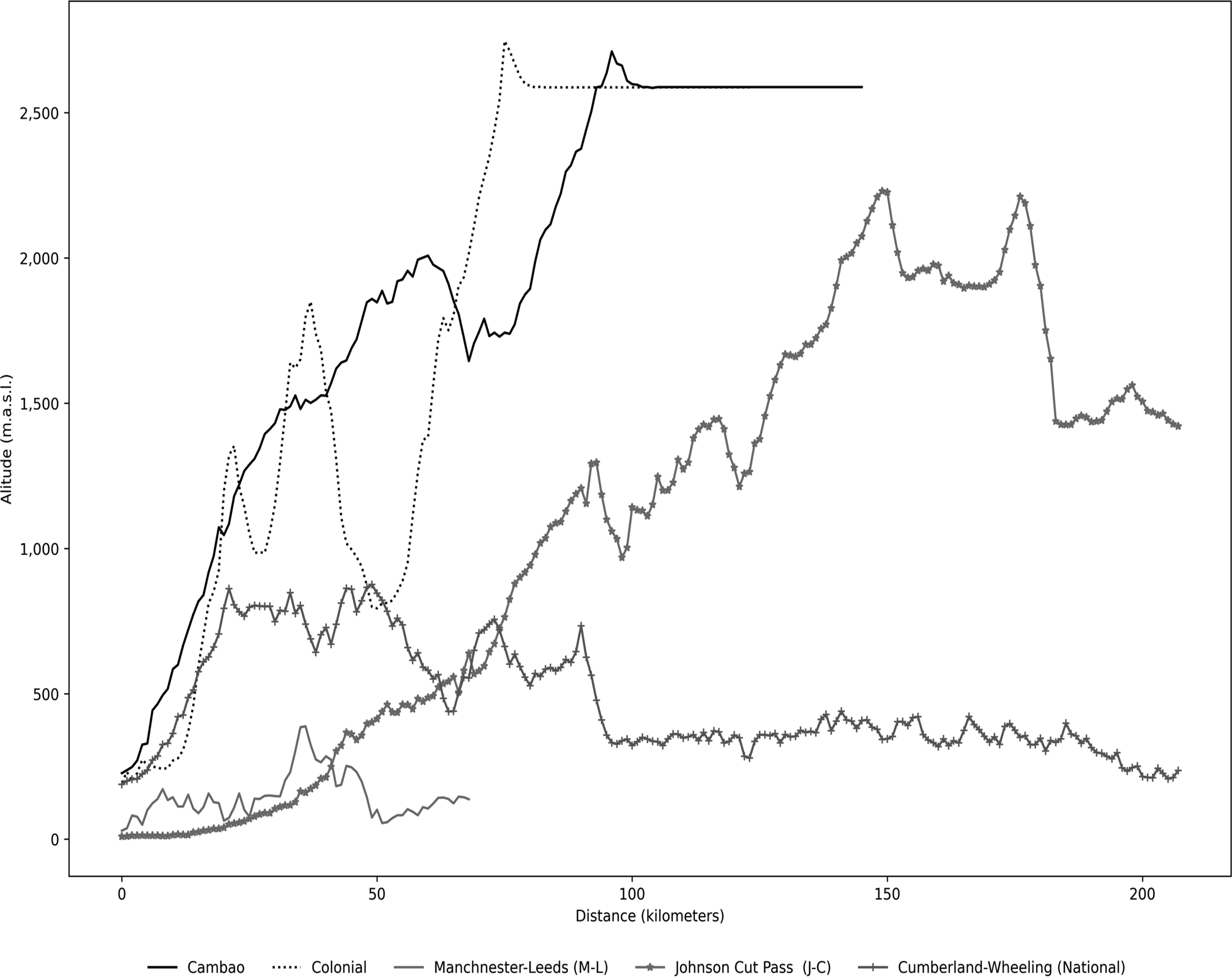
Next, the slope profile of each road was produced. Coordinates for both routes were input into QGIS software to generate a shape file. In turn, the shape file was laid over NASA’s SRTM (90-meter resolution) digital elevation model using the South America Equidistant Conic projection to identify the altitude associated with each point on the shape file. QGIS trail elevation statistics were used to produce the altitude gain by kilometer to calculate each road’s kilometer slope (see Figure 2).
ALTITUDE PROFILE OF COLONIAL, CAMBAO WAGON, AND OTHER SIGNIFICANT MOUNTAIN WAGON ROADS
Notes: The graph compares the altitude profiles of different historical roads. The Colonial road (dotted black line) and the Cambao road (solid black) crossed the Andes, Colombia. The Manchester-Leeds (M-L) road (solid gray) crossed the Pennines, England. The Cumberland-Wheeling (National) road (marked with “+”) crossed the Appalachians, while the Sacramento-Washoe or Johnson Cut Pass (J-C) road (“*”) crossed the Sierra Nevada, both in the United States.
Source: Own construction.

Next, based on the slope, each kilometer was assigned an energy consumption coefficient, e di , estimated in an experiment involving humans and donkeys transporting a load on unpaved, high-altitude roads with varying slopes (Yousef, Dill, and Freeland Reference Yousef, Dill and Freeland1972). We assume that energy requirements of a mule per kilogram of body weight are similar to those of a donkey, in line with veterinary practice.Footnote 7 The daily energy requirements estimated over the colonial and wagon road (humans: 14.90 MJ; mules: 112 MJ) are in line with those typical of humans during vigorous physical activity (12.97–15.57 MJ (FAO 2001 p. 37)) and other equines like horses of the same weight during intense exercise (92–123 MJ; Harris Reference Harris1997, p. 204), suggesting good out-of-sample fit.
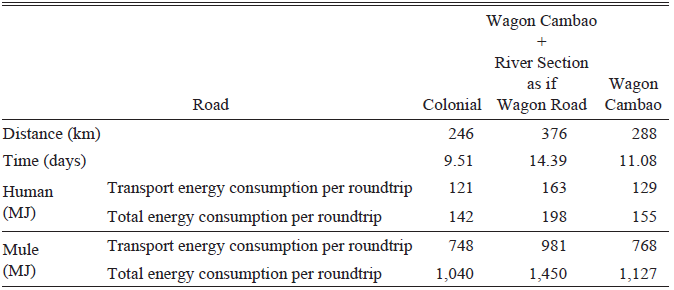
We follow the same thought experiment as in the previous section, but now roundtrip journey time and transport energy costs depend on the road slope profile. Table 3, row 1, shows that a man walks 246 kilometers roundtrip over the colonial mule-pack road with a 14-kilogram load in 9.5 days. His energy requirement is 121 MJ of transport energy during eight workday hours and 142 MJ of total energy (including energy consumption during rest and sleep time) roundtrip.
ENERGY CONSUMPTION FOR HUMAN AND MULE BY ROUTE, ROUNDTRIP

Table 3 Long description
A table comparing energy consumption for human and mule by route for roundtrip journeys. The table has 6 rows and 4 columns. The columns are labeled Road, Distance (km), Time (days), Human (MJ), and Mule (MJ). The rows are labeled with different road types: Colonial, Wagon Road, and Wagon Cambao. Each row provides specific values for distance, time, transport energy consumption per roundtrip, and total energy consumption per roundtrip for both humans and mules. Row 1: Road, Colonial; Distance (km), 246; Time (days), 9.51; Human (MJ) Transport energy consumption per roundtrip, 121; Human (MJ) Total energy consumption per roundtrip, 142; Mule (MJ) Transport energy consumption per roundtrip, 748; Mule (MJ) Total energy consumption per roundtrip, 1040. Row 2: Road, Wagon Road; Distance (km), 376; Time (days), 14.39; Human (MJ) Transport energy consumption per roundtrip, 163; Human (MJ) Total energy consumption per roundtrip, 198; Mule (MJ) Transport energy consumption per roundtrip, 981; Mule (MJ) Total energy consumption per roundtrip, 1450. Row 3: Road, Wagon Cambao; Distance (km), 288; Time (days), 11.08; Human (MJ) Transport energy consumption per roundtrip, 129; Human (MJ) Total energy consumption per roundtrip, 155; Mule (MJ) Transport energy consumption per roundtrip, 768; Mule (MJ) Total energy consumption per roundtrip, 1127.
Sources: Own calculation; see text.
The table also shows that transport energy consumption per roundtrip is lower for the colonial road (142 MJ) than that for the Cambao road, including walking over the path next to the river section from Bodegas to Cambao (198 MJ), as time spent traveling increases from 9 to 14 days (see Column (2)). Even if energy spent walking the river section is excluded, a human consumes more energy walking the Cambao road (Column (3)). These results suggest it was efficient for pre-Columbian indigenous communities to use the straight, steep, short route (like the colonial road) rather than a zigzagging, gentler, and longer one (like the Cambao road). Human physiology literature has identified that we reduce energy consumption walking in a straight-line on steep terrain up to approximately 20 percent grade, compared to taking a longer zigzagging route with lower grades. Thus, human paths tend to follow relatively straight routes (Minetti Reference Minetti1995).
Table 3 shows a mule’s energy consumption over the colonial and wagon routes. Results mirror those for humans.Footnote 8 Thus, it was efficient for the Spanish to build the colonial road over the pre-Columbian human trails, following a straight, steep, short route to perform mule-pack transport.
Transport Energy Cost and Threshold Traffic to Adopt the Cambao Wagon Road
Next, we compute a mule’s energy cost as a function of energy requirements (as opposed to a fixed per night food cost used in Table 1). We calibrated food costs such that a mule’s daily total energy requirement (112 MJ) is met at the daily historical cost ($0.05) (Camacho Reference Camacho1858). The model predicted colonial road freight at 69 percent and roundtrip time at 94 percent of historic values (Online Appendix OA1). Thus, the model provides a good out-of-sample fit.
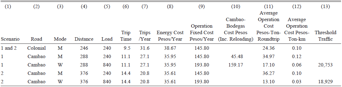
Table 4 presents the baseline results, analogous to those in Table 1. Scenario 1 shows a two-mule-pack on the colonial road covers the 246 kilometer-long round trip, transporting 240 kilograms in 9.5 days and completing 31.6 annual roundtrips. The mule-pack energy (food) cost is $38.67. The mule-pack average operation cost per ton-roundtrip and per ton-km on the colonial road is lower than over the Cambao road; no incentives exist to adopt the wagon road. Using the wheel generates transport cost savings; average operation cost per ton-roundtrip and per ton-km is lower than that with mule-pack over the colonial road. Traffic over 20,753 induces wagon road construction.
MULE-PACK AND WAGON TRANSPORT COST AND THRESHOLD TRAFFIC ON COLONIAL AND CAMBAO ROADS, MODEL CALIBRATED USING CONTEMPORARY INFORMATION AND ESTIMATED ENERGY COSTS

Table 4 Long description
A table comparing transport costs and threshold traffic for mule-pack and wagon transport on Colonial and Cambao roads. The table has 13 columns and 6 rows, including headers. The columns are labeled as follows: (1) Scenario, (2) Road, (3) Mode, (4) Distance, (5) Load, (6) Trip Time, (7) Trips/Year, (8) Energy Cost Pesos/Year, (9) Operation Fixed Cost Pesos/Year, (10) Cambao-Bodegas Cost Pesos (Inc. Reloading), (11) Average Operation Cost Pesos-Ton-Roundtrip, (12) Average Operation Cost Pesos-Ton-km, and (13) Threshold Traffic. The rows present data for different scenarios and modes of transport. Row 1: Scenario 1 and 2, Road Colonial, Mode M, Distance 246, Load 240, Trip Time 9.5, Trips/Year 31.6, Energy Cost Pesos/Year 38.67, Operation Fixed Cost Pesos/Year 145.80, Cambao-Bodegas Cost Pesos (Inc. Reloading) 24.36, Average Operation Cost Pesos-Ton-Roundtrip 0.10, Average Operation Cost Pesos-Ton-km, Threshold Traffic 20,753. Row 2: Scenario 1, Road Cambao, Mode M, Distance 288, Load 240, Trip Time 11.1, Trips/Year 27.1, Energy Cost Pesos/Year 35.95, Operation Fixed Cost Pesos/Year 145.80, Cambao-Bodegas Cost Pesos (Inc. Reloading) 45.48, Average Operation Cost Pesos-Ton-Roundtrip 34.97, Average Operation Cost Pesos-Ton-km 0.12, Threshold Traffic. Row 3: Scenario 1, Road Cambao, Mode W, Distance 288, Load 840, Trip Time 11.1, Trips/Year 27.1, Energy Cost Pesos/Year 35.95, Operation Fixed Cost Pesos/Year 193.80, Cambao-Bodegas Cost Pesos (Inc. Reloading) 159.17, Average Operation Cost Pesos-Ton-Roundtrip 17.10, Average Operation Cost Pesos-Ton-km 0.06, Threshold Traffic. Row 4: Scenario 2, Road Cambao, Mode M, Distance 376, Load 240, Trip Time 14.4, Trips/Year 20.8, Energy Cost Pesos/Year 35.61, Operation Fixed Cost Pesos/Year 145.80, Cambao-Bodegas Cost Pesos (Inc. Reloading) 36.27, Average Operation Cost Pesos-Ton-Roundtrip 0.10, Average Operation Cost Pesos-Ton-km, Threshold Traffic. Row 5: Scenario 2, Road Cambao, Mode W, Distance 376, Load 840, Trip Time 14.4, Trips/Year 20.8, Energy Cost Pesos/Year 35.61, Operation Fixed Cost Pesos/Year 193.80, Cambao-Bodegas Cost Pesos (Inc. Reloading) 13.10, Average Operation Cost Pesos-Ton-Roundtrip 0.03, Average Operation Cost Pesos-Ton-km, Threshold Traffic 18,929.
Notes: Scenario: Threshold traffic is calculated under two different scenarios. Scenario 1 identifies the threshold when adoption of Cambao wagon road and steamer between Cambao and Bodegas is compared to the colonial mule-pack road. Scenario 2 identifies threshold when adoption of Cambao wagon road, including Cambao-Bodegas as wagon road, is compared to the colonial mule-pack road. Road: colonial and Cambao. Mode: Transport mode used; mule-pack (M) or wagon (W). Distance: Roundtrip distance of the road. Load: Load in kilograms carried by mule-pack or wagon. Roundtrip time: Number of days to complete roundtrip journey. Roundtrips: Number of roundtrips per annum. Energy cost: Cost of feeding mules in pesos per annum; calibrated such that cost of meeting mule average daily energy requirements equals cost indicated by Camacho (Reference Camacho1858). Operation fixed cost: Cost of driver, mules (including purchase, depreciation, and finance cost), and wagon in pesos per annum. Cambao-Bodegas cost: Cambao-Bodegas steamer roundtrip transport cost plus transshipment into wagon cost in pesos per annum. Average operation cost pesos ton-roundtrip: ((7) + (8) + (9))/(6))/(4) * 1,000. Average operation cost pesos ton-km: ((7) + (8) + (9)/(6) * (3))/(4)*1,000. Threshold traffic: Traffic that makes transport cost savings equal to construction cost minus net maintenance cost. Observed traffic: Traffic observed over colonial road in 1873.
Source: Own calculations.
Comparing the colonial mule-pack road to the Cambao wagon road, including the Cambao-Bodegas segment (scenario 2), two opposing forces are at work. First, steamer costs are saved, while mules’ and wagons’ annual costs remain approximately equal, reducing the per ton-roundtrip cost. Second, longer trip distance and travel days (after including the Cambao-Bodegas segment), raise per ton-roundtrip cost. Steamer savings outweigh longer trip costs, reducing the threshold to 18,929 tons.
The model, extended to include energy costs, suggests that by the second half of the nineteenth century, transport demand was likely high enough to induce wagon transport adoption (in line with the previous section’s results). Additionally, it highlights that human and mule energy transport costs (without the wheel) are reduced over the colonial straight, steep, short route; this is consistent with the observed route choice of pre-Columbian communities and the Spanish conquistadores.
EXPLORING THE ROLE OF GEOGRAPHY ON TRANSPORT TECHNOLOGY ADOPTION
The model calibrated using contemporary information and energy costs enables a counterfactual analysis to understand the role of geography in transport technology adoption. We explore how dimensions of the model, influenced by geography—road distance and slope—shape its outcomes.
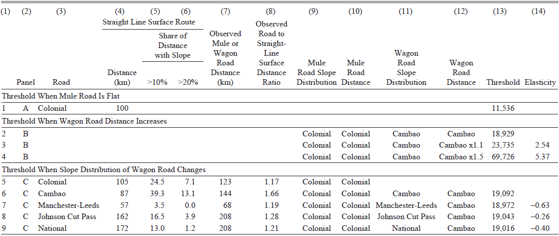
First, we use the calibrated model to examine the simplest case of wagon adoption. If the colonial road had been flat, we assume a wagon road could have been built over the same route by widening and resurfacing it, at the same construction cost per kilometer. This scenario (Table 5, line 1) generates a threshold of 11,536 tons per annum, about 44 percent lower than the baseline scenario 1 in Table 4. Transport technology adoption cost is reduced substantially when topography is flat.
TRAFFIC THRESHOLD CHANGES IN RESPONSE TO SLOPE DISTRIBUTION AND DISTANCE CHANGES

Table 5 Long description
A table comparing traffic threshold changes in response to slope distribution and distance changes. The table has 14 columns and 9 rows, including headers and grouped rows. Column headers are: (1) Panel, (2) Road, (3) Distance (km), (4) Share of Distance with Slope >10%, (5) Share of Distance with Slope >20%, (6) Observed Mule or Wagon Road Distance (km), (7) Observed Road to Straight-Line Surface Distance Ratio, (8) Mule Road Slope Distribution, (9) Mule Road Distance, (10) Wagon Road Slope Distribution, (11) Wagon Road Distance, (12) Threshold, (13) Elasticity. Row labels are grouped into three sections: Threshold When Mule Road Is Flat, Threshold When Wagon Road Distance Increases, and Threshold When Slope Distribution of Wagon Road Changes. Row 1: Threshold When Mule Road Is Flat, Panel 1, Road A, Colonial, Distance 100 km, Threshold 11,536. Row 2: Threshold When Wagon Road Distance Increases, Panel 2, Road B, Colonial, Distance not specified, Threshold 18,929. Row 3: Panel 3, Road B, Colonial, Cambao, Distance not specified, Threshold 23,735, Elasticity 2.54. Row 4: Panel 4, Road B, Colonial, Cambao, Distance not specified, Threshold 69,726, Elasticity 5.37. Row 5: Threshold When Slope Distribution of Wagon Road Changes, Panel 5, Road C, Colonial, Distance 105 km, Share of Distance with Slope >10% 24.5, Share of Distance with Slope >20% 7.1, Observed Mule or Wagon Road Distance 123 km, Observed Road to Straight-Line Surface Distance Ratio 1.17, Mule Road Slope Distribution Colonial, Mule Road Distance Colonial, Wagon Road Slope Distribution Colonial, Wagon Road Distance Colonial, Threshold not specified. Row 6: Panel 6, Road C, Cambao, Distance 87 km, Share of Distance with Slope >10% 39.3, Share of Distance with Slope >20% 13.1, Observed Mule or Wagon Road Distance 144 km, Observed Road to Straight-Line Surface Distance Ratio 1.66, Mule Road Slope Distribution Colonial, Mule Road Distance Colonial, Wagon Road Slope Distribution Cambao, Wagon Road Distance Cambao, Threshold 19,092. Row 7: Panel 7, Road C, Manchester-Leeds, Distance 57 km, Share of Distance with Slope >10% 3.5, Share of Distance with Slope >20% 0.0, Observed Mule or Wagon Road Distance 68 km, Observed Road to Straight-Line Surface Distance Ratio 1.19, Mule Road Slope Distribution Colonial, Mule Road Distance Colonial, Wagon Road Slope Distribution Manchester-Leeds, Wagon Road Distance Cambao, Threshold 18,972, Elasticity -0.63. Row 8: Panel 8, Road C, Johnson Cut Pass, Distance 162 km, Share of Distance with Slope >10% 16.5, Share of Distance with Slope >20% 3.9, Observed Mule or Wagon Road Distance 208 km, Observed Road to Straight-Line Surface Distance Ratio 1.28, Mule Road Slope Distribution Colonial, Mule Road Distance Colonial, Wagon Road Slope Distribution Johnson Cut Pass, Wagon Road Distance Cambao, Threshold 19,043, Elasticity -0.26. Row 9: Panel 9, Road C, National, Distance 172 km, Share of Distance with Slope >10% 13.0, Share of Distance with Slope >20% 1.2, Observed Mule or Wagon Road Distance 208 km, Observed Road to Straight-Line Surface Distance Ratio 1.21, Mule Road Slope Distribution Colonial, Mule Road Distance Colonial, Wagon Road Slope Distribution National, Wagon Road Distance Cambao, Threshold 19,016, Elasticity -0.40.
Source: Own construction.
Second, when the Cambao road distance increases by 10 and 50 percent (leaving all else equal, including the mule-pack road distance), the threshold level is 23,735 and 69,726 tons per annum (see lines 3 and 4). The implied elasticity is 2.54 and 5.37 percent, respectively. When the Cambao wagon road distance is 85.9 percent longer, the Cambao and colonial per ton-roundtrip cost equalize; the advantage of using the wheel is eroded. Hence, the calibrated model is relatively sensitive to increasing wagon road distance.
Third, we can also replace the Cambao wagon road slope distribution with that of another mountain wagon road, leaving all else equal. Since identifying the relevant theoretical counterfactual road slope distribution is challenging, we use the distribution of the first wagon road to cross a significant mountain range and that have been digitized, including the Manchester-Leeds (M-L) road that crossed the Pennines, England in 1735 (Bogart, Rosevear, and Satchell Reference Bogart, Rosevear and Satchell2017), the Cumberland-Wheeling (National) road that crossed the Appalachians, United States in 1818; and the Johnson Cut Pass (J-C) road that crossed the Sierra Nevada, United States in 1861 (National Park Service n.d.).
A simple and intuitive way to get a sense of the geographical challenge across these different regions is to measure the straight-line surface (including mountains) distance between origin and destination of each road, as well as the share of kilometers with a slope higher than 10 percent and higher than 20 percent. The longer the distance, the more challenging it is to connect two regions; and the higher the share of distance over 10 or 20 percent slope, the steeper the mountains and the more challenging it is to locate and build a wagon route to connect two regions.
The colonial road connects Bogotá to Bodegas. Its straight-line surface distance (over the mountains) is 105 kilometers, with almost a quarter of the distance with slopes of more than 10 percent and 7.1 percent of the distance with a slope of more than 20 percent (see line 5). The mule-pack road built is 123 kilometers long, a ratio of 1.17 compared to the straight-line surface distance. Additionally, it exhibits absolute grades of 10 to 20 percent more frequently than the four wagon roads examined. Interestingly, the four wagon roads, the Cambao, M-L, National, and J-C roads, have a similar slope distribution (Online Appendix OA3). Independently of the underlying mountain chain (Andes, Pennines, Appalachian, or Sierra Nevada) and the differences in straight-line distance length and share of distance with slopes higher than 10 or 20 percent, which signal important differences in each of the road’s underlying landscape, it was possible for contemporaries to locate and build a wagon route by performing zigzagging and increasing route distance to reduce grades higher than 10 percent. In turn, even if the four roads crossed very different geographies, all four wagon roads exhibit similar slope distribution.
Another key difference across these roads is the ratio of observed route distance to the straight-line surface distance. For the Cambao road, this ratio is 1.66, significantly higher than the values for the M-L (1.19), National (1.21), and J-C (1.28) roads. This reflects the Colombian Andes’ ruggedness, where finding gentler slopes requires more extensive zigzagging, increasing both road distance and construction costs. Consequently, the threshold traffic required to justify building a wagon road in the Colombian mountains is higher than in regions with more favorable terrain.
Next, we use the calibrated model, replace the Cambao wagon road slope distribution with that of these other wagon roads, and produce technology adoption thresholds. The baseline uses the Cambao road distance, including the river segment. However, instead of assuming that the river segment is flat, as we have in Table 4, scenario 2, we use the Cambao road mountain segment slope distribution over the full road distance to make the comparison to the historically significant mountain roads fairer. This raises the threshold level in line 5 slightly higher to 19,092. When the alternative slope distributions are used, the thresholds are between –0.63 and -0.26 percent lower than the baseline level. As the slope distributions of the Cambao and the historically significant mountain roads are very similar to each other, the implied threshold levels are also similar.
In sum, the demand required to induce wagon road construction to connect Bogotá to the Magdalena River would have been substantially lower had the terrain been flat. Even if the Cambao wagon route slope distribution was similar to that of other wagon roads, the required demand would likely have also been lower had the Colombian landscape looked like other mountain chains in the Americas and Europe, as proxied by their lower wagon road to straight-line surface distance ratio. This confirms impressions that Colombia’s geography is comparatively more rugged and that it raises overland transport technologies’ adoption costs.
Additionally, even if it is not possible to offer general findings based on the sample of roads examined, the origin-destination distances examined in this case study do highlight that Bogotá was not further from water transport compared to other locations in the Americas. Perhaps the breakup of the Andes at Colombia’s southern border creates a highly rugged topography, but it also funneled a river that crossed the country from south to north and offered cheap river transport at a shorter distance than other parts of North America or most of the massive, undivided Andean range.
CONCLUSIONS
The invention and use of wheeled transport for long-distance trade are important technological achievements of antiquity. However, the Andes adopted wagon transport only after a long and puzzling delay, in the late nineteenth century.
We document the history of the first use of wagon transport for long-distance trade in the Andes: The Cambao wagon road connected Bogotá to the Magdalena River in 1885.
We propose the first hypothesis to explain the slow adoption of the wheel in the Andes. When human or animal transport is used on mountainous terrain, a straight, steep, short route reduces energy transport costs. In turn, selection of this route implies a switching cost to adopt wagon transport: a new, gentler, zigzagging, and longer route needs to be located and a new road built. Construction of a new road only becomes cost-effective when traffic is high enough to offset these expenses through savings generated by wagon transport.
We examine this hypothesis using a calibrated threshold technology-adoption model of the Cambao wagon road. Even if the timing of the construction of the wagon road is likely driven by multiple factors, including state capacity, road location uncertainty, political competition, and railway optimism, the calibrated model helps to understand why incentives, influenced by human and animal physiology, geography, and transport demand, may have played a key role. It is likely that only in the second half of the nineteenth century was observed traffic high enough to allow wheeled transport to reduce transport unit costs sufficiently to compensate for wagon-road construction costs. This result is robust to significant changes in model parameters.
Our interpretation of the model results is that Pre-Columbian communities, trading low volumes and using human transport, selected straight, steep, short routes to locate their trails and reduce transport energy and costs. The Spanish conquistadores, in the face of a vast new landscape, limited traffic, and the collapse of the indigenous population that continued well into the mid-eighteenth century, chose to continue using the straight, steep, short routes, despite having brought pack animals to the Americas and knowing how to build and operate wagon roads. Population levels only rebounded during the second half of the nineteenth century. Since population is a key determinant of transport demand, it led to high enough transport demand to induce wagon road construction and wheeled transport adoption at some point in the late nineteenth century. Wagon transport demand rose further as Bogotá imported more voluminous and heavier capital goods.
The model suggests that while Andean topography did delay adoption of wheeled transport compared to flat landscapes, it probably also imposed a stronger barrier to the adoption of transport technologies than the topography of other mountain chains. Although it was feasible to build wagon roads with comparable slope profiles across diverse mountain chains, the Colombian wagon road required a longer route relative to the origin-destination straight-line surface distance. Route searching, road construction and maintenance, and transport costs were higher in the Colombian Andes.
The breakup of the Andes at the southern border of the country created a rugged topography that increased transport adoption and operation costs and likely retarded Colombia’s development. But it also funneled rivers, shortening access to water transport to many locations. The Andean breakup seems as much a curse as a blessing.
Our approach is a first attempt to examine the puzzle of slow wagon adoption in the Andes and opens new directions for future research. Results highlight how incentives derived from the interaction between topography, human and animal physiology, and transport demand shaped slow wagon adoption in the Andes. Future research may use this framework to examine the role that rugged topography and long origin-destination distances played in the non-adoption of wagon transport in high transport demand places like colonial Potosí, Panama, or Mexico City-Veracruz. A natural extension is to study adoption of wagons and railroads as competing overland transport technologies with different adoption threshold levels to better understand leapfrogging from mule to railroad in many places in the Americas. A different direction is to explore other important events in the adoption of wagon transport, like its spread around the Mediterranean during the Roman Empire, or the timing of adoption reversals in Africa and Asia.
Appendix Table 1 PARAMETER VALUES AND SOURCES

Source: Compiled by the authors.


 Open access

