


1. Early Undercurrents
1.1. Introduction
Used generically, ‘extrusion flow’ describes a velocity field in which the horizontal velocity increases with depth, so that underlying ice flows out or is ‘extruded’ from beneath overlying ice. This concept has had a colorful and checkered history. In order to appreciate its life story, some understanding of the evolution of thought on glacier flow is necessary. Interiors of glaciers are difficult to observe directly, and over the past three centuries the shortage of data stimulated creative theories about glacier flow, as scientists attempted to fill this gap in understanding. At the risk of sounding like a closet taxonomist, I will describe three variants of extrusion flow that have appeared in the glaciological literature.
The first variant, which we might call ‘free extrusion flow’, was the idea that some glaciers and ice sheets, when viewed on length scales that were greater than their thickness, contained regions with strong undercurrents. As an analogy, we might think of mortar that extrudes from under a heavy brick as the brick settles into position; however, in the ice sheet, the ‘brick’ was just made of stiffer ice, and the ‘mortar’ was softer ice. This mechanically questionable concept was formally called ‘extrusion flow’ by Reference DemorestMax Demorest (1941a, Reference Demorest1942, Reference Demorest1943). The second form could be called ‘capped extrusion flow’. On length scales short compared to the ice thickness, a relatively soft basal layer can move around bedrock bumps more rapidly than the usually more rigid ice above it (the ‘cap’), which provides a restraining force (e.g. Reference CarolCarol, 1947). The third form could be called ‘rotational extrusion flow’; however, I will call it simply ‘rotational flow’, because ‘extrusion’ generally implies some shape change. A glacier with a concave surface and bed can undergo motion resembling a rigid rotation about a horizontal axis above the glacier surface. The lower ice, being farther from the rotation axis, moves faster. This behavior has been associated with some cirque glaciers (e.g. Reference Gibson and DysonGibson and Dyson, 1939).
In order to appreciate the context of the extrusion flow debate, it is helpful to first review the development of glacier flow concepts. Until the mid-19th century, there was little consensus on how glaciers moved. Both the mechanism of flow and the spatial pattern of flow were unknown.
1.2. Mechanisms of glacier motion
1.2.1. Sliding
Because hand samples of ice appear to be a brittle solid, naturalists hypothesized modes of flow that could be compatible with rigidity. Reference AltmannJohann Georg Altmann (1751) and Reference GrunerGottlieb Sigmund Gruner (1760) suggested that glaciers moved forward by sliding over their bases as rigid blocks. Movement around corners had to be accommodated by melting or brittle failure. Horace-Bénédict de Saussure also endorsed the idea of motion by sliding, in his four-volume treatise (Reference Saussurede Saussure, 1779-96) about his alpine travels. Reference HopkinsWilliam Hopkins (1845) supported the sliding theory and proposed that glaciers could turn corners by slip along en echelon faults within the ice. Some later observers thought that glaciers moved entirely by slip on fracture surfaces or faults within the ice itself. For example, in 1894, Thomas Chrowder Chamberlin observed shear planes and thrust features in stratified ice in the termini of some Greenland glaciers. Reference ChamberlinChamberlin (1895) then suggested that individual sedimentary layers moved as cohesive units, possibly bending and sliding relative to one another, but maintaining their identity throughout their flow history (i.e. deforming like a deck of playing cards). The layering that Chamberlin observed may have been a secondary foliation, rather than the initial bedding, and the thrusts that he observed were probably of local extent. However, both shearing and ductile yielding play some part in glacier flow under various conditions (e.g. Reference NyeNye, 1951).
1.2.2. Dilatation
Johann Jakob Scheuchzer, a physicist from Zürich, proposed the dilatation theory of glacier flow. According to the dilatation theory, meltwater flowed into the interstices and cracks in the ice each day, then froze at night. The volume expansion upon freezing then pushed the lower tongue of the glacier forward (Reference ScheuchzerScheuchzer, 1723).
In 1840, Louis Agassiz published Études sur les glaciers (Reference AgassizAgassiz, 1840). This work is also available in English translation by Albert V. Carozzi (Studies on glaciers: Reference Agassiz and CarozziAgassiz, 1967). Agassiz originally accepted Scheuchzer’s dilatation theory, and this assumption led him into several pitfalls. Because there was more meltwater near glacier margins than near the center of glacier channels, and often more crevasses as well, Reference AgassizAgassiz (1840, p.86) assumed that glaciers flowed more rapidly near their edges. He also thought that glaciers did not flow in winter when there was little or no meltwater (Reference AgassizAgassiz, 1840, p. 212). When basal meltwater was present, however, Agassiz thought that the basal ice would flow more rapidly than the surface ice. This mechanically improbable pattern of deformation, ‘extrusion flow’, lived on for over a century. To Agassiz’s credit, he himself corrected some of these errors by actually measuring glacier motion. His stake network at Unteraargletscher, Switzerland, in 1841-42 moved during the winter, and transverse lines became convex downstream (Reference AgassizAgassiz, 1842). Between 1840 and 1847, when he published his second book Nouvelles études et expériences sur les glaciers actuels (a collection of his previously published papers about glaciers: Reference AgassizAgassiz, 1847), he conducted one of the first extensive and scientific observation programs on glacier movement. In 1847, he again speculated about extrusion flow based on the progressive tilt of stratigraphic layers (Reference AgassizAgassiz, 1847, p.270), but he realized that this was mere conjecture (see Reference BattleBattle, 1951). He was actually imagining a rotational flow. Observations by Agassiz and confirmed by Reference ForbesJames David Forbes (1845, p. 441; 1859, p. 69) revealed that the velocity at the glacier surface tended to be largest near the firn line; it did not increase monotonically from bergschrund to terminus as the dilatation theory predicted. By embedding minimum thermometers at depth up to 10m in the glacier (Reference AgassizAgassiz, 1842), Agassiz also came to realize (Reference TyndallTyndall, 1872, p. 156) that temperate glaciers could not extract enough heat from water in deep cracks to cause it to freeze as the dilatation theory required, because the ice was already at the melting temperature.
1.2.3. Viscous flow
One of the earliest writers to suggest that ice flowed as a viscous or ductile substance, in spite of the apparent rigidity of small specimens, was A.C. Reference BordierBordier (1773). In his book entitled Picturesque journey to the glaciers of Savoy, he observed that ice behaved like ‘softened wax, flexible and ductile to a certain point’, which flowed downward ‘after the manner of fluids’ (quoted by Reference TyndallTyndall, 1872, p. 157).
Louis Rendu, a Catholic canon who subsequently became bishop of Annecy in France, pointed out the similarities of glacier flow and river flow (Reference RenduRendu, 1840; translation by A. Wills: Reference RenduRendu, 1874), and predicted that a glacier should move most rapidly (1) at the surface and (2) near the center of its channel. His observations of crevasse patterns and the displacement of surface features (Reference RenduRendu, 1874, p. 85) substantiated the second prediction. Rendu attributed to ice
-
a kind of ductility which enables it to mould itself to its locality, to thin out, to swell, and to contract as if it were a soft paste (Reference RenduRendu, 1874, p. 71).
He further described the similarity between rivers and glaciers:
-
there is in the Glacier des Bois and a river a resemblance so complete that it is impossible to find in the glacier a circumstance that does not exist in the river. In currents of water, the velocity is not uniform throughout their depth; the friction of the bottom, that of the sides, the action of obstacles cause a variation in the velocity which is undiminished only towards the middle of the surface. Now the mere inspection of the glacier is sufficient to prove that the velocity of the center is greater than that of the sides. (Reference RenduRendu, 1874, p. 85)
Rendu postulated that ice could fracture and flow when the pressure exceeded a certain amount. He realized that further experiments to measure the solidity of ice were necessary. We now know that the ductility of ice depends on the stress deviator, rather than on pressure. Rendu’s appreciation of the importance of stress was a major advance, but the misconception about the role of hydrostatic pressure persisted into the 20th century and played a role in extrusion flow theory.
In 1841, Agassiz invited James David Forbes, Professor of Natural Philosophy at Edinburgh University, to join him at Unteraargletscher. Forbes became interested in glacier flow, and wrote two books on the subject, Travels through the Alps of Savoy (Reference ForbesForbes, 1843) and Occasional papers on the theory of glaciers (Reference ForbesForbes, 1859, a collection of previously published papers). Reference ForbesForbes (1845, p. 162) and Reference AgassizAgassiz (1842) both noticed the foliated structure of glacier ice. Forbes described narrow bands of hard, clear ice a few centimeters thick, alternating with bands of bubbly ice; he called this ‘the ribboned structure’ or ‘the veined structure’ of glaciers. He suggested (Reference ForbesForbes, 1845, p.406) that the hard clear bands represented crevasses which had filled with meltwater, frozen and been stretched by differential flow. On Mer de Glace, Chamonix, France, Forbes saw that the ribboned structure formed spoon-shaped surfaces, concave upward, and dipping up-glacier. He realized (Reference ForbesForbes, 1845, p. 402) that the ribboned structure was not stratigraphic but was caused by, and could be used to map, the glacier flow. Describing these structures, he wrote:
-
their figure at once gives the idea of fluid motion, freest in the middle, obstructed by friction towards the sides and bottom (Reference ForbesForbes, 1845, p. 406).
Forbes introduced theodolite surveying techniques to observations of glacier motion. His theodolite observations of differential motion, even in areas free of crevasses (Reference ForbesForbes, 1845, p. 438), led him to conclude of glaciers, that
-
the extreme inequality of motion of the central and lateral parts of glaciers is the best direct proof of the very considerable plasticity of their mass (Reference ForbesForbes, 1845, p. 445).
Forbes is widely credited with ‘the viscous theory’ of glacier flow; he frequently emphasized the viscous or plastic nature of glacier flow, although he did not differentiate the two constitutive behaviors in the way that we would today (a viscous substance deforms at a rate proportional to the applied deviatoric stress, whereas a plastic substance is rigid up to a characteristic stress, above which it offers no resistance to yielding).
1.2.4. Regelation
John Tyndall, Professor of Natural Philosophy at the Royal Institution in London, published two books about glacier physics. Glaciers of the Alps (first edition 1860; Reference TyndallTyndall, 1896 (fourth edition)) was divided into two sections: the first was a travelogue and mountaineering guide, and the second, observations and discussion of glacier flow. His second book, The forms of water (Reference TyndallTyndall, 1872), resulted from a Christmas lecture series for young people in 1871 at the Royal Institution.
Tyndall looked to the microscopic level for an explanation of glacier flow. He was an advocate of the ‘regelation flow theory’. In 1850, Michael Faraday had found that two clean surfaces of melting ice, when brought into contact, would freeze together, and James Thomson Bottomley of Glasgow University (Reference BottomleyBottomley, 1872) had performed the classic regelation experiment, in which a weighted wire passed through a block of thawing ice in one half-hour, leaving the block of ice in one piece;the pressure of the wire reduced the melting point of the ice under the wire, allowing the ice to melt, and the water subsequently refroze above the wire. Reference TyndallTyndall (1872, p. 165) compressed blocks of ice in moulds, showing that, when the ice was near 0°C, the ice fractured, then was reunited by regelation into a new block of a different shape, and, if the pressure was applied carefully, the shape could be changed without total fracture. Since glacier ice is under pressure due to the weight of overlying ice, he concluded that
-
by the slow and constant application of pressure the ice gradually moulds itself to the valley, which it fills (Reference TyndallTyndall, 1872, p. 166).
Tyndall envisioned ice as a brittle material crushed by pressure and shear stresses, and reunited by regelation after minor rearrangement of the fragments. The process of regelation is important in basal sliding, and, as Tyndall realized, in crevasse closure (Reference TyndallTyndall, 1872, p. 166) and in the transformation of firn to ice (Reference TyndallTyndall, 1872, p. 165), but it is an incomplete explanation of the internal deformation of glaciers;for example, flow is observed in ice masses that are too cold for regelation to occur.
Tyndall frequently criticized Forbes’ viscous theory (e.g. Reference TyndallTyndall, 1896, p.327). Forbes’ theory had obvious weaknesses, but then, so did Tyndall’s regelation theory. Because of this controversy, some glaciologists thought of the glacier flow problem as simply a choice between the viscous model and the regelation model. This impeded the development of a complete description of flow, and physical appreciation of the patterns of flow.
For further discussion on glacier-deformation theory in the late 19th century, see the extensive contemporary review by William Luttrell Reference RogersRogers (1888). A century later, Reference ClarkeClarke (1987) and Reference Walker and WaddingtonWalker and Waddington (1988) offered updated perspectives.
1.3. Patterns of glacier motion
Once glaciers were generally understood to move by some kind of ductile flow, it became possible to theorize (or to speculate) on the subsurface flow patterns. For example, because of his adherence to the dilatation theory, Louis Reference AgassizAgassiz (1840) originally thought that flow was faster next to glacier margins than on the center line of a glacier, and greater at depth than at the surface. In 1841, following instigation of a quantitative survey program at Unteraargletscher in 1841-42, and his discussions with Forbes, Agassiz found that his transverse stake lines became convex downstream (Reference AgassizAgassiz, 1842, Reference Agassiz1847; Reference TyndallTyndall, 1896, p. 273).
Forbes also made detailed observations of glacier motion on Mer de Glace, detecting movement over times as short as 1 hour (1845, p. 133), and showing that the ice generally moved steadily (1845, p. 444), rather than with a stick-slip motion. In 1842, he confirmed Agassiz’s observation that the ice at mid-channel flowed more rapidly than ice near the glacier margins; their results were published nearly simultaneously.
Measuring variations with depth was more challenging, and measurements were necessarily incomplete. Reference AgassizAgassiz (1840, p. 166) cited Franz Joseph Hugi (1830, plate 3) who had noted that empty moulins did not remain vertical as they moved downstream from the places where they had formed. Their tops moved farther downstream than their interiors, implying that the faster velocities were at the surface.
In the absence of boreholes whose tilt could be monitored, Forbes wanted to measure the speed at several heights on a steep face of a glacier. He was concerned that stresses associated with spreading laterally and turning corners in a glacial valley could affect the flow pattern, so he sought a location where the flow was more-or-less rectilinear. He found such a location at the steep terminal face of Glacier des Bois (Mer de Glace), where he installed three markers, labeled (1), (2) and (3) in Figure 1, which shows a frontal view and a longitudinal section through the terminus (Reference ForbesForbes, 1859, p. 172). As expected, the higher markers moved farther in a 24 hour period (Fig. 2).
Terminus of Glacier des Bois (Mer de Glace), showing locations of markers (1), (2) and (3) used by Forbes to demonstrate that deep ice moved slower than the overlying ice. (a) Longitudinal profile; (b) frontal view. From Reference ForbesForbes (1859).

Displacements over a 24 hour interval as measured by Forbes (×) in 1846 (Eleventh Letter, Reference ForbesForbes, 1859) at the terminal face of Mer de Glace (where it was called Glacier des Bois), and by Reference TyndallTyndall (1872) (o) on a steep right margin of Mer de Glace below Mont Tacul. Dashed curves were produced with Equation (1).

A steep ice wall close to 50 m high was exposed on the right margin of Mer de Glace where it turns left at Mont Tacul. Expecting that vertical variations in velocity u as a function of height z above the bed on this steep face would also be representative of velocities at similar elevations within the glacier, Tyndall placed three stakes on the wall, and observed their motion over a day. As shown in Figure 2, the top stake moved fastest, and the bottom stake moved slowest, as expected (Reference TyndallTyndall, 1872, p.80). In spite of their different locations relative to the glacier span and central axis, the patterns in horizontal velocity u(z) at both locations were remarkably similar, and consistent with the pattern in Equation (1),

which is the exact solution for flow of a parallel-sided ice slab (Reference NyeNye, 1952a), with ice thickness h, surface velocity u s, basal-slip velocity u b = u s/2 and flow exponent n = 3 (Reference GlenGlen, 1952, 1955).
In more general patterns of flow, Equation (1) also arises from the shallow-ice approximation (e.g. Reference Fowler and LarsonFowler and Larson, 1978).
1.4. Theory and observation
1.4.1. Two solitudes
The decade 1840-50 saw the beginnings of experimental glaciology, and in the following six decades the physical and mathematical foundations were developed for many of the concepts of glacier flow as we understand them today. However, there was an ongoing isolation between physicists, who wanted to reduce glaciers to their simplest common factors in order to understand fundamental processes, and naturalists (e.g. glacial geologists) who wanted to make many measurements in order to classify all the complexities in the natural world as a prelude to understanding glaciers as components of complex systems. As section 1.2 suggests, in the absence of data, many early ideas on glaciers were speculative. As Tyndall expressed it:
-
In science thought, as far as possible, ought to be wedded to fact. This was attempted by Rendu, and in great part accomplished by Agassiz and Forbes. (Reference TyndallTyndall, 1872, p. 160)
However, the gap persisted through the 19th century. Richard Mountford Deeley was the Chief Mechanical Engineer (CME) of Midland Railway; he was also a scientist and a Fellow of the Geological Society (FGS) and a Member of the Institution of Civil Engineers (MlnstCE). He had broad interests and expertise, ranging from railway-locomotive design to Pleistocene fossils, to Pleistocene geology, to glacier flow. Reference DeeleyDeeley (1895) lamented that
-
Although, ever since the classical researches of J. D. Forbes on the phenomena presented by the Swiss glaciers were published, it has been recognized that glacier-ice behaves like a viscous liquid, and flows from high to low levels much in the same way as does a river of water, it is apparent that many who have interested themselves in the subject of glacier-flow, and have written rather dogmatically on the subject, have not clearly realized the nature of the phenomenon. Very contradictory and erroneous conclusions have consequently been arrived at...
-
Our knowledge of the subject is by no means due to recent discovery. The viscous flow of liquids – and glacier-ice behaves as a very viscous liquid – was worked out by Poiseuille and Coulomb The discoveries of these workers are quite sufficient to enable us to work out the more important phenomena presented by glacier- flow from first principles. Indeed, had sound physical theory been adhered to by all writers on the subject of glacier erosion and transport, the mistakes so many have fallen into might have been avoided.
If Deeley had only known, more mistakes were yet to be made, as glaciologists struggled to understand their developing subject. Seventy-four years later, in the preface to the first edition of Physics of glaciers, Stan Reference PatersonPaterson (1969) noted,
-
in glaciology, as in other branches of science, there is a place for both the theoretical and the experimental approach. But the two should be coordinated; the experiments designed to investigate specific problems.
Awareness of this persistent isolation between physical process and taxonomy of systems should provide helpful context as we explore the origins of extrusion flow. Both world wars interrupted glacier research, and the tenor was noticeably different when research restarted in earnest each time. Major developments in glaciology between 1840 and 1914 (the start of World War I) were made by physicists and mathematicians. However, between the two world wars, the emerging energy was found in the geological community as the field of glacial geology blossomed. The extrusion-flow theory was born in this period. Since World War II, there has been a renewed focus on glacier physics; the extrusion-flow theory died early in this current era.
1.4.2. The first era of glacier physics, 1840-1914
The viscous theory was ultimately accepted by most physicists and mathematicians with an interest in glaciers. It was mathematically tractable, and great progress could be made. Reference DeeleyDeeley (1895) clearly distinguished the difference in behaviors of viscous materials and plastic materials in response to stress, and derived solutions for viscous flow in cylindrical channels and on inclined planes. Reference DeeleyDeeley (1908) used these results together with estimates of glacier thicknesses and observed flow rates at ten locations on four glaciers in the Alps to estimate the bulk viscosity of polycrystalline ice as 1.25 × 10¹⁴ poise, or 1.25 × 10¹³ Pa s, and this value was later used by Demorest. (Reference Deeley and ParrDeeley and Parr (1913) proposed the name poise for the c.g.s. unit of viscosity, after Poiseuille who had demonstrated its constancy in various fluids flowing in pipes.) There was a large scatter in their derived values; we now know that the viscosity of ice is stress-dependent. Reference DeeleyDeeley (1895) was also aware that the viscosity might not be constant.
Some of the earliest mathematical modeling of glacier flow appeared at the end of the 19th century. Reference ReidHarry Fielding Reid (1896) and Sebastian Reference FinsterwalderFinsterwalder (1897) calculated streamlines through steady glaciers. Reference FinsterwalderFinsterwalder (1907) solved the continuity (mass conservation) equation to find glacier thickness changes; this procedure is the basis of modern models of glaciers and ice-sheet evolution.
Adolf Reference Blümcke and HessBlümcke and Hans Hess (1899) carried out one of the most comprehensive glacier surveys of that era. They measured ablation rate, surface altitude and ice velocity along a series of transverse profiles on Hintereisferner, Austria. In addition, they used borehole information coupled with the Reference FinsterwalderFinsterwalder (1897) kinematic theory to estimate the ice thickness.
Boris Weinberg, a physicist at the University of Odessa, is perhaps best known today for his visionary ideas on magnetically levitated high-speed trains in vacuum tunnels (‘vactrains’). However, he also studied slower-moving objects. Reference WeinbergWeinberg (1907) estimated the viscosity of Hintereisferner by using the equations for viscous flow in an elliptical channel to approximate the observations of Blumcke and Hess (1899). Reference Deeley and ParrDeeley and Parr (1913, Reference Deeley and Parr1914) also used those Hintereis data in two outstanding papers. Reference Deeley and ParrDeeley and Parr (1913) found a solution to the Poisson equation for viscous flow in a uniform channel having a cross section more general than an ellipse. They showed that, compared with Reference WeinbergWeinberg’s (1907) result, this type of channel (which they called ‘Parr’s curve’) could give an improved fit to the observed flow of Hintereisferner.
Deeley and Parr also addressed the difficult question of separating basal slip from internal shear deformation; the amount of basal slip also impacts the depth pattern of velocity within a glacier. They estimated the basal sliding velocity by assuming it was proportional to the basal shear stress, and inversely proportional to the frictional resistance. They pointed out that, since ice must flow around some obstacles on the bed, the flow and sliding questions were connected. In their 1913 paper, Deeley and Parr noted that flow is controlled primarily by the slope of the ice surface, rather than by the slope of the glacier bed. Their second paper (Reference Deeley and ParrDeeley and Parr, 1914) focused primarily on the basal sliding problem. They presented a conceptual model of sliding that is remarkably similar to the ‘tombstone’ model put forward independently by Johannes Weertman in 1957 (Reference WeertmanWeertman, 1957). Deeley and Parr envisioned flow by regelation around small basal obstacles. Instead of representing the glacier bed by a plane with an array of cubes with a characteristic separation (the Weertman model), Deeley and Parr represented the glacier bed by a plane covered by an array of pyramids with a characteristic base dimension and slope angle. In both models, the parameters could be adjusted to balance the downslope component of gravity against the resistance offered by the uphill faces of the obstacles. Deeley and Parr pointed out that ice moved past large obstacles, channel curves and other irregularities by viscous flow; however, they did not envision the enhancement of flow due to stress concentrations as pointed out by Reference WeertmanWeertman (1957).
Reference Deeley and ParrDeeley and Parr (1914) tested their ideas on slip by measuring the sliding rate of a loaded piece of ice on an inclined, grooved rock slab in their laboratory, noting that the slip rate decreased as the temperature dropped below 0°C. They expected this result from the regelation mechanism.
By 1914, the consensus among glaciologists was that glaciers moved by some sort of ductile flow, with an additional contribution from basal motion at temperatures where regelation could operate. Solutions had been obtained for glacier flow, by assuming that the ice was a viscous fluid, comparable to setting n = 1 in Glen’s flow law (Reference GlenGlen, 1952, 1955), for relatively simple glacier geometries, with assumptions similar to the shallow-ice approximation (e.g. Reference Fowler and LarsonFowler and Larson, 1978) that is widely used today. The viscosity of temperate glacier ice had been estimated to be 1012-1013 Pa s, with the recognition that ice was probably not in fact a perfectly linear material; its viscosity could be variable.
1.4.3. The era of glacier geology, 1918-50
After World War I, European focus appears to have turned to glacier measurement and inventory. The former International Glacier Commission was revived as a part of the International Association of Scientific Hydrology, and hundreds of glaciers were described in its annual reports (Reference Matthes and MeinzerMatthes, 1942). In North America and the UK, the momentum in glacier research appears to have passed to the glacial geologists, who focused primarily on interpretation of glaciated landscapes as windows into Earth history. In 1945, Noel E. Odell (who had been a climber and geologist with the 1924 Mallory Everest expedition) observed,
-
while there is in all a very large body of students of glacial geology, that is to say of the actual effects of ice masses upon the land surface, there are at work remarkably few glaciologists, whose particular study is the physical condition and constitution of those masses, even in countries where glaciers are a normal feature of the landscape (Reference OdellOdell, 1945 ).
Most of these practitioners of glacial geology were content to accept general wisdom about the physics of glacier motion, or to extend it in (apparently) logical ways as necessary. Appeal to extrusion flow to account for observed geological and glaciological features was one such temptation. Because the Earth is complicated, Earth scientists are often trained to look beyond the simple answers. With glaciers, this produced the uneasy suspicion that perhaps there might be more to glacier flow than the obvious analogy to river flow. As expressed by Gerald Seligman, founding President of the International Glaciological Society, in 1947,
-
In the middle of the last century, Agassiz, Tyndall and others showed that a glacier flowed faster at its centre than at its margin. Partly from experiments, and partly from the assumption that it behaved like a river, it became generally accepted that it also flowed faster at the surface than lower down. This belief was held until ten or fifteen years ago although search through earlier literature shows that evidence was accumulating which might disprove this. (Reference SeligmanSeligman, 1947 )
In this era, two independent lines of evidence (presented by Max Demorest and by Rudolf Streiff-Becker) converged to suggest that another mode of flow, extrusion flow, might also exist. Although both lines of evidence were ultimately shown to be flawed, nevertheless their confluence reinforced the idea that the earlier pioneers had missed something important about glacier flow.
Because of work by Reference GlenJohn Glen (1952, Reference Glen1955, Reference Glen1958) and Reference NyeJohn Nye (1953), we now appreciate that strain rate increases and effective viscosity of ice decreases when the deviatoric stress increases. However, several related misconceptions were apparently widespread in the 1918-50 period.
-
1. In some geological circles, the term ‘pressure’ was apparently commonly used as a synonym for stress, without the recognition that pressure is a very special sort of stress, i.e. isotropic (equal in all directions). Furthermore, it was appreciated that ice softened at warmer temperatures and under higher shear stress. However, this was translated into the first well-known but incorrect ‘fact’ that ice softened under increasing pressure. (Reference Johnston and AdamsJohnston and Adams (1913) had pointed out the error in that concept.)
-
2. This misconception led logically to the second well- known ‘fact’ that ice was always softer at greater depths in glaciers.
-
3. There was apparently a widespread misunderstanding of the terms ‘deformation rate’ (i.e. velocity gradients) and ‘flow’ (i.e. velocity), which were apparently sometimes thought to be synonyms. This misunderstanding produced the third incorrect ‘fact’ that ice moved faster where pressure was higher, rather than that ice strained (changed shape) faster where differential stresses were higher.
Sometimes, as Deeley had feared, these misconceptions could lead to difficulties (e.g. with conservation laws). Appeal to extrusion flow to account for observed geological and glaciological features was one such temptation. For example, Sydney Ewart Reference HollingworthHollingworth (1931) published a major paper on the glacial history of Edenside in the north of England, describing the interactions of ice caps in the Lake District and ice coming south across the Solway Firth from Scotland. In order to reconcile ice-flow directions indicated by drumlins and by erratic boulders, Hollingworth suggested that the ice had the overturning circulation shown in Figure 3 (Reference HollingworthHollingworth’s (1931) Fig. 2). Although the reversed pattern of flow at Orton looks surprising to modern glaciologists, to Hollingworth it was the least unlikely way to resolve the geological data. Probably the observations could also be explained by a temporal pattern of changing flow direction that was more complex than those that Hollingworth considered.
Proposed flow pattern in ice cap over northern English Lake District, based on drumlin shapes and transport of erratic boulders. From Reference HollingworthHollingworth (1931). Reproduced with permission of the Geological Society.

Reference HolmesChauncey D. Holmes (1937) studied the deep valleys in the Finger Lakes region of upstate New York. He argued that the pronounced valleys had been carved not by fluvial action, but by ice which eroded headward and cut away cols on the Allegheny Plateau. He noted that downward flow associated with the heavy precipitation expected in ice- age New York probably would have reduced the thermal gradient in the upper layers of the ice cover, cooling the upland bedrock below the freezing point, thereby protecting it from erosion. In order to explain the focused erosion in the valleys, Holmes argued that the thick ice in the valleys flowed more vigorously than the ice on the uplands, because in the valleys
-
the melting point isogeotherm (as determined by the existing pressure) was doubtless at or near the contact of the glacier and its bedrock floor.
Following the third misconception above, he also attributed the relatively vigorous flow in the valleys to the higher pressure there, rather than to higher shear stress:
-
Hence other conditions being equal, the greatest tendency to flow would be where the pressure is greatest … Therefore a favorable temperature as well as greater pressure gave to the basal ice the optimum requirements for flow.
Holmes also stated that
-
In the forward movement of the ice, the weight of the accumulating snows, pressing downward, would cause the ice beneath it to move laterally in the direction of least pressure: that is, in the direction of the surface slope of the glacier.
Holmes did not say whether the ice above the fast-flowing basal ice in the valleys also moved rapidly; however, statements such as those above led some glaciologists to consider his work to offer support for the extrusion flow theory. For example, Gerald Seligman apparently was drawn to these ideas. In assessing the pros and cons of the extrusion flow theory, Reference SeligmanSeligman (1947) suggested that Holmes’s work supported the idea that
-
wherever the pressure of the ice is increased, the line of maximum flow tends to become lower in the glacier and the glacier bed is deepened … I think … that steps, valley lakes and corrie tarns, and perhaps even fjords can be more adequately accounted for by the extrusion flow hypothesis.
In other developments, Reference AleschowAleschow (1930) reported extrusion flow in a cirque glacier in the Urals, and Reference Gibson and DysonGibson and Dyson (1939) invoked a rotational extrusion flow to explain the dip of stratification planes in Grinnell Glacier, Montana, USA.
William S. Reference CarlsonCarlson (1939) measured the flow of some outlet glaciers in the Upernivik region of northeast Greenland in 1931, showing that speed was fastest in the center of the glaciers. His field partner was a young graduate student from the University of Michigan, Max Demorest. Carlson had intended to also measure the vertical distribution of velocity on some glacier margins, as Forbes and Tyndall had done at Mer de Glace (Figs 1 and 2). However, in the 1939 paper, Carlson noted that the data on the vertical variation of velocity had not yet been analyzed. It appears that World War II intervened, and those data on vertical distributions of velocity were never published, although after the war Carlson went on to become president of four different universities (Delaware, Vermont, State University of New York, and Toledo, Ohio).
Erich Dagobert von Reference DrygalskiDrygalski (1938), Reference Hess and GutenbergHans Hess (1933, p. 113) and Francois Reference Matthes and MeinzerMatthes (1942) thought that the west Greenland outlet glaciers were fed from the ice sheet by extrusion flow. Reference Matthes and MeinzerMatthes (1942) had been influenced by the writings of Max Demorest on ice dynamics in Greenland (Reference DemorestDemorest, 1937), and extrusion flow (Reference DemorestDemorest, 1941a, Reference Demorest1942).
The most ardent and respected proponents of extrusion flow in the 20th century were Max Demorest and Rudolf Streiff-Becker. Demorest argued for extrusion flow based on dynamics (force considerations), whereas Streiff-Becker argued for extrusion flow based on kinematics (conservation of mass). The confluence of these two independent lines of reasoning created a more convincing argument than either of the two arguments independently.
When I first reviewed the history of glacier flow as an over-confident and under-insightful graduate student (Reference WaddingtonWaddington, 1982, appendix 17), I thought that Demorest and Streiff-Becker were the woefully uneducated villains of the extrusion-flow story. Now, however, with 30 more years of experience, I tend to view them rather differently, as flawed heroes of glaciology, struggling to make sense of the world that they observed, without the knowledge that we possess about glacier mechanics today.
2. Birth and Life of Free Extrusion Flow
2.1. Max Demorest
2.1.1. Early career and achievements
Max Demorest was a rising young star of glaciology and glacial geology shortly before World War II. As a student, he studied meteorology and later investigated glacier flow and its contribution to geological history in northwest Greenland with the University of Michigan (Reference DemorestDemorest, 1937). He obtained his PhD at Princeton in 1938, and in 1940 and 1941 carried out further glacier research at Yale (Reference FlintFlint, 1943). Demorest was clearly a young scientist with broad interests and a quick enquiring mind. A few examples of his work should illustrate this.
Reference DemorestDemorest (1938) mapped striation patterns and their relation to bedrock ledges and topography in the previously glaciated area in front of Clements Glacier, Montana, and recognized that they represented streak lines in the ice flow when the area was covered by ice. He was able to infer that the basal ice had moved as a ductile fluid, even at the scale of individual abrading rock tools; the ice did not fail on shear faults over the tops of obstacles. In response to objections that a substance weak enough to flow should be incapable of holding tools firmly enough and steadily enough to produce striations, Demorest argued that
-
The fallacy lies in supposing that the cutting tools must necessarily be firmly held… [T]he important thing in the cutting of striae is that heavy tools should move across a bedrock surface. … In the case of a glacier, the pressure that causes flowage is in part a pressure adding weight to the tools such that even a small pebble may become effective in producing striae. (Reference DemorestDemorest, 1938, p. 721)
Although technically he used the terms ‘pressure’ and ‘weight’ incorrectly in this context, Demorest apparently thought that the rock tools creating striations were not held rigidly in the ice (like grit in sandpaper) but were pushed hard onto the bedrock by viscous ice that slowly flowed around them. This idea is now the key concept behind the Stokes flow model for abrasion (Reference HalletHallet, 1979), in which it is that very difference in velocity between the ice and the tool that creates the huge forces that cause abrasion.
Consistent with work of a flawed hero, Demorest also made some dubious or incorrect statements in that paper, as he strove to bridge the solitudes between physical process and taxonomy. First, his taxonomy background showed, as he tried (Reference DemorestDemorest, 1938, p. 703) to classify the continuum of glacial striations into four categories.
Second, by observing currently glaciated and recently deglaciated areas, geologists (e.g. Reference Matthes and MeinzerMatthes, 1942) had recognized that ice generally exceeded some minimum thickness before noticeable glacial erosion occurred. De- morest recognized that determining this depth could provide a clue to the constitutive parameters of ice that controlled its flow. Using his observations of striations at Clements Glacier, Demorest estimated that the critical depth was approximately 50 m, producing a critical pressure of approximately 4 × 10⁵ Pa, or 4 bar, for glacier flow. Although he came very close to a correct and useful result, he had succumbed to incorrect fact number 3 (section 1.4.3): deformation rate actually depends on shear stress rather than on pressure. His map of the terrain at Clements Glacier showed a slope of approximately α = 0.25. If he had simply multiplied his basal pressure (ρgh = 4 bar) by the glacier slope α, he would have obtained a very good estimate ρghα = 1 bar for the yield stress of glacier ice, if the ice were represented as a plastic material.
Third, he invoked the Bernoulli effect to suggest that the ice pressure was reduced where ice moved more rapidly, and this reduced pressure helped to draw ice up and over bedrock obstacles. I suspect that a reviewer of the paper may have pointed out that the Bernoulli effect requires the fluid to be inviscid and to have measurable kinetic energy, which is definitely not the case for glacier flow. Reference DemorestDemorest (1938) included a footnote justifying his argument by analogy:
-
Analogy to an example of this sort may be objected to on the grounds that kinetic energy plays a role in the mechanism of such rapidly moving fluids, while in such slowly moving substances as ice kinetic energy is too small to be considered. Nevertheless, the relation between differential pressure and differential flow is clearly expressed, and the example is used for that reason.
When World War II interrupted his research, Demorest was also working on field instrumentation, although the work was never published. In an abstract for the December 1941 Geological Society of America (GSA) meeting, Demorest (1941c) described a new lightweight field apparatus with which he could make 15 cm diameter thin sections of glacier ice, and photograph them in the field. His sections could survive for 15-30 min of study, even on warm summer days.
The existence of the Greenland ice sheet was problematic for some scientists of this period. How did it flow with such a low slope? And if the center did not flow, why did snow not build up continually there? Meteorologist William Herbert Hobbs of the University of Michigan, one of Demorest’s early mentors, thought that a stable high-pressure system (‘the glacial anticyclone’) persisted over Greenland, and this high-pressure system blocked cyclonic storms that would otherwise bring moisture to the interior (e.g. Reference HobbsHobbs, 1921, Reference Hobbs1926, Reference Hobbs1934). Hobbs mounted several meteorological expeditions to Greenland to test this idea. When Part II of the expedition report was published (Reference HobbsHobbs, 1941), Reference DemorestDemorest (1941b) published a thoughtful review in the American Journal of Science that clearly showed he was also a careful meteorologist. For example, he understood and recommended that further studies of sublimation and deposition on the ice sheet were needed before the mass balance could be definitively estimated. The Alfred Wegener Greenland Expedition (e.g. Reference SorgeSorge, 1933) had shown that there was significant net accumulation in central Greenland, contrary to Hobbs’ anticyclone ideas; however, some Michigan team members and co-authors of the expedition reports may have been reluctant to recognize that the growing evidence did not fully support the glacial anticyclone concept. In his review, Demorest pointed out that it was inconsistent to adhere to the permanent anticyclone concept in which all cyclones were blocked from Greenland, when the authors of the report also documented warm downslope winds on the ice-sheet slopes, which they interpreted as föhns driven by cyclonic winds crossing a high-elevation barrier. Demorest noted,
-
To the reviewer, the amazing thing is that cyclonic disturbances which find an effective barrier in the ice sheet, should nevertheless be able to ‘draw’ air from all the way across the barrier! (Reference DemorestDemorest, 1941b, p. 776)
Notwithstanding his own Bernoulli principle analogy in 1938, Demorest was not a fan of nonquantitative science based on analogies instead of on physics. Oscar Diedrich von Engelnwas Professor of Geology at Cornell University. Based on work by Otto Flückiger, Reference Engelnvon Engeln (1937, Reference Engeln1938) had published the idea that glacier flow had a naturally wavy pattern, and just as water in a stream produced bed ripples, glaciers produced bedforms such as roches moutonnées. Citing work by von Helmholtz on waves on interfaces between differing fluids, Reference Engelnvon Engeln (1938, p. 437) suggested that
-
[The] … ubiquitous roche moutonnée form … is simply the mold of the wave train in the ice.
(In glaciers, the two fluids were possibly clean ice and debris-laden ice.) The waves in the flow were purported to produce spatial variations in ‘gross attack’, and by comparison the competence of the bedrock was unimportant. Reference DemorestDemorest (1939) criticized this concept. He realized that inertial effects were key to the flows described by von Helmholtz, whereas inertial effects were negligible in glacier flow. Taking a fluid-mechanics perspective, Demo- rest pointed out that wavy flows required turbulence and the viscosity of the fluid was very important. He argued that in order to undergo the transition from laminar to turbulent or ‘wavy’ flow, a fluid with a viscosity μ had to flow at a characteristic transition velocity v. Although he did not use the term ‘Reynolds number’, his scale argument was equivalent to finding the ice-flow velocity v that would produce a Reynolds number Re = (ρvL)/μ of order unity. For a characteristic length scale L (e.g. ice thickness L ≈ 100 m), density ρ (900kgm-3) and viscosity μ (e.g. 1.25 × 10¹³ Pas from Reference DeeleyDeeley, 1908), Demorest demolished the ‘grossness of attack’ theory of erosion by pointing out that flow would be laminar unless the ice velocity v approached the speed of light. Demorest’s reductio ad absurdum argument now seems ironic, in light of the fact that his own extrusion flow theory was later devastated by a similar speed-of-light argument by Reference NyeJohn Nye (1952b).
2.1.2. Demorest’s extrusion flow
Demorest is the scientist most clearly associated with the term ‘extrusion flow’, because he defined it in his publications (Reference DemorestDemorest, 1941a, Reference Demorest1942, Reference Demorest1943) in the specific context of polar ice sheets. His interests that led him to extrusion flow appear to have begun on the University of Michigan expedition to northwest Greenland with W.S. Carlson. The lead scientist, W.H. Hobbs, thought that the relatively flat central regions of the ice sheet were essentially motionless, because he thought that accumulation rate was negligible there. His ‘glacial anticyclone’ hypothesis explained the lack of accumulation. As Demo- rest noted in his review (Reference DemorestDemorest, 1941b), the glacial anticyclone was actually not as strong as Hobbs thought, and there was significant snowfall, even on the highest parts of the ice sheet. That discovery created another problem for a thoughtful young student such as Demorest, who wanted to understand the mechanics of the flow. If he still accepted that the surface slope was too low to drive flow, how could accumulating ice be evacuated from the ice-sheet interior without evident flow? This apparent dilemma led to his extrusion-flow hypothesis.
When Demorest published his own research from that northwest Greenland project (Reference DemorestDemorest, 1937), he was already formulating a distinction between ‘gravity flow’ in the outlet glaciers descending through the mountain barriers, and ‘pressure-driven flow’ in the inland ice, which moved primarily horizontally. He suggested that
-
the ice moves out radially from below the centers of greatest accumulation, the rate of movement in the various directions being dependent on the different pressure gradients. As the ice is forced out from beneath these centers, the higher ice moves down to take its place. (Reference DemorestDemorest, 1937, p. 45)
Although Reference SeligmanSeligman (1947) interpreted this as a statement of extrusion flow, it could also describe downward flow in which the upper ice is carried along by the ice below. I think that Demorest’s concept of extrusion flow may not yet have been fully formulated.
Demorest fully accepted the fact that when glaciers flowed downhill, the fastest velocities were at the surface, and the slowest velocities were at the bed, as amply demonstrated by Forbes and Tyndall (Fig. 2), and as predicted by viscous flow models (e.g. Reference WeinbergWeinberg, 1907; Reference Deeley and ParrDeeley and Parr, 1913; Reference SomiglianaSomigliana, 1921a, Reference Somiglianab, Reference Somiglianac, Reference Somiglianad). Demorest called this ‘gravity flow’ (see Fig. 4a, which was published in his 1942 paper). The key idea was that the ice motion in gravity flow had a downward component of motion aligned with gravity, so the motion was driven directly by gravity.
(a) Demorest’s ‘gravity flow’ category was a standard viscous-flow profile consistent with much previous work. Because of basal drag, flow was fastest at the surface. In Demorest’s classification, gravity flow operated where slopes were relatively steep. RO illustrated a later position of the line NO for ice with uniform viscosity, and QO showed a later position if the viscosity increased with height. (b) ‘Extrusion flow’ was driven by horizontal pressure gradients, and was thought to operate in regions with flat beds and very low surface slope. The stiff surface ice moved slowly, and a fast undercurrent (at level b) in the ductile ice near the bed was able to carry off any excess ice accumulating near the center of an ice sheet. Adapted from Reference DemorestDemorest (1942). Reprinted by permission of the American Journal of Science.

Demorest thought that gravity flow would not work in the ice-sheet interior, because the motion there was essentially horizontal, i.e. orthogonal to the force of gravity. That perceived problem led him to the idea that there had to be another type of flow, which he called ‘pressure-controlled flow’. Horizontal ice motion was driven by horizontal pressure gradients, rather than directly by gravity. He had expressed this idea of two kinds of flow in his 1937 paper about northwest Greenland glaciers (Reference DemorestDemorest, 1937). These ideas probably evolved into extrusion flow around 1940, in order to resolve the apparent problem of ice evacuation from central Greenland.
Consistent with taxonomic training in geology, in his abstract for the GSA meeting of 1941 (Reference DemorestDemorest, 1941a), he proposed a four-part classification scheme for flow regimes. The four categories were extrusion flow, blocked extrusion flow, gravity flow and blocked gravity flow. The complete description of the classification system appeared in Reference DemorestDemorest (1942, Reference Demorest1943).
‘Extrusion flow’ was the primary ‘pressure-controlled’ type of flow. Reference DemorestDemorest (1942) illustrated extrusion flow with the diagram reproduced here as Figure 4b. Even though the surface slope was gentle, there would be a pressure gradient directed horizontally with a uniform value everywhere along the vertical line ac. He argued that the deep ice was much softer than near-surface ice because the ice pressure was higher, and therefore the deep ice flowed fastest.
-
The result is movement of the ice, but the amount of movement, unlike the differential pressure, is not uniform from bottom to top. This is because ice plasticity increases with depth so that the given pressure causes greater deformation near the bottom than near the top. Consequently the surface of deformation is shown by its trace abc. Within the upper part of the glacier, the ice is sufficiently non-plastic to resist deformation and at the base frictional retardation occurs, but between these two parts the rate of flow is a function of plasticity; that is, a function of the weight of overlying ice. (Reference DemorestDemorest, 1942, p.36)
Unfortunately, in this argument Demorest apparently succumbed to all three of the incorrect ‘facts’ outlined in section 1.4.3. The plasticity or softness does not increase with pressure. If ice were a perfectly viscous fluid, the softness would be uniform; however, we now know (Reference GlenGlen, 1952, Reference Glen1955) that softness increases with shear stress (in this case, horizontal forces acting on horizontal internal surfaces). Shear stress does increase with depth, so a generous reader might attribute that misstatement to imprecise terminology. However, even if the upper part of the ice sheet was stiffer, it would not be motionless. Demorest did understand the difference between deformation rate and velocity, and the fact that the upper ice was simply carried along by the ice below. In his description of gravity flow, he had stated:
-
the upper surface is relatively non-plastic, and therefore capable of resisting the weak near-surface shear stresses. Thus it is not subject to internal differential shearing; yet it does move through a greater downstream distance than any other part of the glacier, for its total movement is the sum of all underlying differential movements. (Reference DemorestDemorest, 1942, p. 37)
Why he did not apply the same logic in describing his extrusion flow remains a mystery.
The ‘obstructed flow’ categories were meant to describe situations where bedrock topography or slower-moving ice got in the way and forced the streamlines to rise away from the bed. For example, in ‘obstructed extrusion flow’, the point of maximum speed (b in Fig. 4b) would rise; if it reached the surface, ‘extrusion flow’ had transitioned into ‘gravity flow’. In Demorest’s taxonomy, gravity flow could also be obstructed, for example near a glacier terminus where rapidly flowing ice overtakes thinner and therefore slower ice. Today we would call this ‘compressional flow’.
From the perspective of 2010, Demorest’s flow taxonomy system appears to be based on a failure to realize that ‘gravity flow’ and ‘pressure-controlled flow’ are equivalent descriptions of the same flow. The only difference is in the perspective of the observer describing the flow, i.e. in the coordinate system. Information about the velocity field can be obtained from the balance of forces on a typical block of ice of unit width across the flow (e.g. the stippled area in Fig. 5). Forces acting in the direction of the x-axis are pressure forces F u on the upstream face, F d on the downstream face, traction F t on the top surface, and a shear force F b on the bottom. In addition, F g is the gravitational body force. Because any acceleration of the block is negligible, these forces sum to zero, i.e.
Horizontal force balance in a glacier with surface S(x) and bed B(x). (a) In vertically aligned coordinate system (x, z), resistive viscous force F b on lower surface balances pressure-gradient forces F u and F d on the vertical sides. (b) In coordinate system (x′, z′) aligned with glacier surface, resistive viscous force F b balances gravitational body force F g. The resulting flow field is the same in both (a) and (b)


To a good approximation, pressure P in the ice is lithostatic as assumed by Demorest, i.e. P(x,z) = ρg(S(x)-z). For an observer using a coordinate system that is aligned vertically as in Figure 5a, the forces per unit width are:


The force F t on the top surface is zero because the glacier surface is stress-free. The pressure force is higher in magnitude on the upstream face; this observer sees ‘pressure-controlled flow’. The net pressure force is balanced by a shear stress τ on the bottom surface. Equation (2) shows that τ must be

Now, from the perspective of an observer in a coordinate system (indicated by primes) aligned with the surface S(x) as in Figure 5b, the forces per unit width are


This observer sees ‘gravity flow’. In this framework, the acceleration component (gdS/dx) acts in the|x′ direction on a mass (ρhΔx′) per unit width, and this gravitational body force F g is resisted by shear stress τ on the bottom surface. From Equation (2), τ is also given by

Representing the ice as a quasi-viscous fluid with a local viscosity μ,eff at the level z 0 in Figure 5, the shear stress τ can be related to the vertical gradient of the horizontal velocity u through a constitutive relation,

Putting Equation (7) into Equation (4) or (6) produces the same velocity gradient at corresponding locations, i.e.

and, therefore, the same velocity field. For the Greenland ice sheet, the surface slope dS/dx is small, the increments Δx and Δx′ are equivalent, and Demorest’s distinction between ‘pressure-controlled flow’ and ‘gravity flow’ can be seen to be semantic rather than physical.
Although Demorest had a geological background, and was trained in the observe-and-classify camp (see section 1.4.3), in his research he attempted to bridge the solitudes, by bringing physics and taxonomy together. In his publications, he sought to find physical explanations for the complex geological and glaciological phenomena that he observed. He addressed the question of glacier flow from a dynamics perspective and he invoked ‘the principles of fluid mechanics’ in his publications. He had apparently been exposed to concepts of continuum mechanics; his publications showed intuitive insights into shear stress and pressure- gradient forces, strain rate and viscosity. These words did not show up often in contemporary glaciology papers. However, as he reached across this scientific gulf, he apparently lacked the background in mechanics to follow up and check some of his insights.
2.1.3. Demorest’s demise
In 1942, the US Air Force was ferrying many airplanes from the USA to the UK, with stops at Gander, Newfoundland; Narsarssuak (now Narsarsuaq) or Søndre Strømfjord (now Kangerlussuaq), Greenland; and Keflavik, Iceland. The flight over the Greenland ice sheet was the most perilous leg of the journey. Because of his previous Greenland field experience, Demorest, then a lieutenant in the US Army Air Force (USAAF), was selected by William S. Carlson (his old field companion from northeast Greenland in 1932) as a senior officer in a search-and-rescue team. The team’s mission was first to establish a coastal base camp in southeast Greenland and then to establish stations on the ice cap from which small teams could travel by snow machine to rescue fliers whose planes went down on the ice. Reference WadeWade (1946) included photos and maps from the mission.
In November 1942, Demorest led a team attempting to rescue the crew of a Boeing B-17 Flying Fortress that had gone down in a crevassed area. Shortly after he and his crew reached the downed airplane, Max Demorest and his snow machine broke through a snow bridge and fell out of sight in a crevasse more than 50 m deep. It was impossible to rescue him. Four more men died before the B-17 crew were rescued: one air crewman in a crevasse, and three aviators aboard a Coast Guard Grumman Duck rescue plane that crashed on the ice near Køge Bugt (south of Ammassalik) in bad weather shortly after leaving the B-17 crash site. The remaining B-17 crew members spent five and a half winter months on the ice sheet before they were finally rescued. Their ordeal and rescue has entered military lore, and Max Demorest was one of its principal players. The full story was told by Reference CarlsonCarlson (1962).
Demorest’s final paper (Reference DemorestDemorest, 1943) was published posthumously. Two of the leading glacial and periglacial geomorphologists of the 20th century, Richard Foster Flint and A.L. (Linc) Washburn, handled the final stages of publication. When he published his textbook Glacial geology and the Pleistocene epoch in 1947 (Reference FlintFlint, 1947), Flint dedicated it to Max Demorest:
-
To the memory of MAX DEMOREST 1910-1942 Outstanding glaciologist, excellent field companion, generous and thoughtful friend, who died to save the lives of others. November 30, 1942
An obituary in the American Journal of Science, written by Reference FlintFlint (1943), concluded:
-
His mind was forever turning over glacial problems, but the one that lay nearest to his heart was the problem of the origin, the form, and the movement of the Greenland ice sheet, which he had come to know on earlier expeditions. He could have chosen no better nor more appropriate grave than that vast and silent ice field to which he had devoted so much constructive thought.
Max Demorest may yet be disturbed in his silent ice field. The US military aims to recover the remains of all MIA (missing in action) servicemen. In September 2010, the US Coast Guard sent a team equipped with ground-penetrating radar (GPR) to search for the Grumman Duck that crashed on the B-17 rescue mission. Using hot water, in September they drilled their first GPR target, which turned out not to be the missing Grumman Duck (http://coastguard.dodlive.mil/index.php/2010/09/duck-hunt-taking-stock/). The ‘Duck Hunt’ team plans to return to investigate other targets in their search area. A story on the expedition appeared in the New York Times on 21 September 2010 (http://www.nytimes.com/2010/09/21/science/21greenland.html).
In 1942, the air crew and Demorest’s team mates noted the location of the crevasse in relation to the B-17 Flying Fortress when Demorest went down. If the Coast Guard Duck Hunt team is successful in locating and recovering the Duck, their attention will probably turn next to finding the B-17 and Max Demorest.
-
During the 4 month B-17 rescue in 1942, 3 people fell into hidden crevasses … two were killed and are still out there. One (USAAF LT Max Demorest) fell thru approx 100 yards from the crashed B-17. We’re working on locating him (the B-17, then him). (http://forums.military. com/eve/forums/a/tpc/f/415197802/m/4210095852001)
We are left to wonder whether Max Demorest would have preferred to be recovered, or to stay in his silent ice field. Demorest was 32 years old when he died, and he would have been 100 this year (2010).
2.2. Rudolf Streiff-Becker
2.2.1. Career and achievements
While Max Demorest proposed a dynamical basis for extrusion flow, Rudolf Streiff-Becker thought that extrusion flow must exist on kinematical grounds. When growing up in Austria and Switzerland in the late 19th century, Rudolf showed talent as an artist, and aspired to be a naturalist. However, he was also trained as an engineer and he spent two decades developing a family business in Brazil. After returning to Switzerland, he devoted time to mountaineering and the study of glaciers. Although he was not formally an academic, he published 32 papers between 1922 and 1957 (Reference HaefeliHaefeli, 1960). His interests and curiosity were broad;in addition to papers on ice movement, he also published on glacial erosion and ice flow (Reference Streiff-BeckerStreiff-Becker, 1934), glacial landforms (Reference Streiff-BeckerStreiff-Becker, 1941, Reference Streiff-Becker1949), moulins and potholes (Reference Streiff-BeckerStreiff-Becker, 1951), firn structures (Reference Streiff-BeckerStreiff-Becker, 1952), water flow through glaciers (Reference Streiff-BeckerStreiff-Becker, 1948), snow penitents (Reference Streiff-BeckerStreiff-Becker, 1956), and periglacial processes and patterned ground (Reference Streiff-BeckerStreiff-Becker, 1949). His artistic talent complemented his writing, and he incorporated pen-and-ink sketches in his papers. In one striking example published in the Journal of Glaciology (BGS, 1947) he had prepared two drawings of the same landscape to illustrate the difference between the terms ‘glacierized’, which described terrain that was currently inundated by glaciers (Reference Wright and PriestleyWright and Priestley, 1922, p. 134), and ‘glaciated’, which described terrain that had been modified by ice in the past. Figure 6 is another example of his abilities as a scientific illustrator.
(a) Stratigraphy and flow in a valley glacier. (b) In a valley glacier, maximum ice velocity was expected to be strongly focused in the basal layers where the bed was concave, and rising to higher levels where the bed was convex. Near the terminus, the maximum speed was expected at the surface. (c) Similar patterns were expected in an ice sheet or ice cap, because its lower layers were expected to be plastic. From Reference Streiff-BeckerStreiff-Becker (1942) and Reference SeligmanSeligman (1947).

Streiff-Becker was particularly interested in the glaciers of the Alps of Glarus Kanton, eastern Switzerland. In 1916, he began to measure summer and winter mass balances at two points on Claridenfirn, a glacier on the northeast flank of Claridenhorn. The record from his upper marker at 2900 m (labeled Obere Boje in Fig. 7) is now the oldest continuous series of direct summer and winter mass-balance measurements in the world, and accordingly is a valuable dataset for climate change studies (Reference Müller-Lemans, Funk, Aellen and KappenbergerMüller-Lemans and others, 1994; Reference Vincent, Kappenberger, Valla, Bauder, Funk and Le MeurVincent and others, 2004).
Claridenfirn showing Obere Boje (i.e. upper marker) at 2900m where velocity and mass balance were measured. Streiff- Becker used region ABCD for continuity calculation. Adapted from Reference Streiff-BeckerStreiff-Becker (1938) and Reference SeligmanSeligman (1947).

2.2.2. Streiff-Becker’s extrusion flow
In addition to measuring the seasonal balances at Claridenfirn, Streiff-Becker measured a surface velocity of 14 m a-1 at his upper marker. He also estimated the ice thickness along CD in Figure 7 by extrapolating the planes of sedimentary beds back up under the firn from location F. Figure 8a shows his inferred profile, which reached a maximum depth of 110 m.
(a) Streiff-Becker’s estimated depth profile along CD in Figure 7, and contours of steady-state velocity required to carry away the upstream accumulation. The velocity of 14ma–1 along the surface had been measured at Obere Boje (Fig. 7). (b) The estimated velocity–depth profile at the deepest point (110 m). (c) Expected velocity–depth profile if the true depth was actually 200 m. (d) Velocity profile if the true depth was 270 m, as measured by Reference Funk, Bösch, Kappenberger and Müller-LemansFunk and others (1997). Only a small amount of extrusion flow would be required, even if Streiff-Becker’s flux estimate was correct. Adapted from Reference Streiff-BeckerStreiff-Becker (1938) and Reference SeligmanSeligman (1947). Panel (d) added by E.D.W.

Because the surface elevation at Obere Boje did not change between 1916 and 1934, Streiff-Backer expected that the ice flux through the ‘gate’ CD in Figure 7 would roughly equal the total annual mass balance in the region ABCD. His reported net balance rate measured at Obere Boje was 3.167 m a-1, with a density of approximately 650 kg m-3. Multiplying the annual surplus measured at Obere Boje by the area 1.09 × 10⁶m2 of region ABCD produced an input rate of 3.45 × 10⁶m3a-1. No ice crossed AB or BC, which were edges of the glacier. Streiff-Becker thought that no ice crossed AD, which was a topographic ridge on the glacier surface. Streiff-Becker’s estimated cross section at CD (Fig. 8a) had an area of 6.8 × 10⁴ m2, so even if the entire cross section moved by plug flow at the speed 14 m a-1 measured at Obere Boje, the flux through that gate was only 0.95 × 10⁶m3a-1, or less than one-third of the amount that Streiff-Becker had calculated for steady state. To account for the persistent steady-state surface of Claridenfirn, Streiff-Becker proposed that a strong undercurrent must exist as shown in Figure 8b.
Since the net upstream mass balance, the cross section of the gate at CD, and the surface speed at that gate were measured or estimated, we can define a dimensionless ‘extrusion index’ I E given by

where A firn is the area of the firn basin ABCD, ḃ is the net balance rate, and h(x) and u s(x) are the ice depth and surface velocity along the gate CD. When I E is greater than unity, some degree of extrusion flow is required for steady state. For Streiff-Becker’s depth profile in Figure 8a, the extrusion index is I E = 3.6. Streiff-Becker had confidence in his maximum depth estimate of 110m along the CD profile. However, to demonstrate that the extrusion flow was strongly indicated, he repeated the calculation supposing that the depth under CD was as much as 200 m, which was presumably an outrageously great depth; as Figure 8c shows, strong extrusion flow was still necessary; the extrusion index in this case would be I E = 2.0, i.e. still significantly greater than unity. This result was apparently robust and convincing. Perhaps, in the presence of an astonishing but apparently inescapable result, Streiff-Becker was simply following the advice of Sherlock Holmes (in Arthur Conan Doyle’s ‘The Sign of Four’, 1890):
-
Eliminate all other factors, and the one which remains must be the truth.
Because Streiff-Becker was confident about his 110 m depth estimate, it was then reasonable to invoke extrusion flow to explain features of the glacial landscape. His illustration (reproduced in Fig. 6) shows extrusion flow in overdeepenings, where fast basal flow and basal shear presumably contributed to erosion. The locus of fastest extrusion flow would then rise out of overdeepenings; he attributed the persistence of riegels to this pattern, which removed rock tools from the bed, preventing erosion. We now appreciate that extrusion flow is unnecessary to create this effect; flowlines can rise away from the bed in compressive flow as ice slows down on an uphill bed slope (e.g. as pointed out by Reference NyeNye, 1951).
Gerald Seligman presented Demorest’s concepts of extrusion flow and Streiff-Becker’s data to English-speaking glaciologists at the General Meeting of the British Glacio- logical Society (the predecessor of the International Glaciological Society) on 26 April 1946;the lecture and subsequent discussion were published in the first issue of the Journal of Glaciology (Reference SeligmanSeligman, 1947). Seligman concluded his article with
-
I have put forward the extrusion flow hypothesis. While there is much to be said in its favour and while it is supported by many eminent glaciologists, my personal opinion is that it cannot be finally accepted without further observational research. Nevertheless, the observations and the arguments are sufficiently compelling to justify serious consideration.
In the subsequent discussion, two critical questions were raised:
-
1. Could some ice leave the area ABCD through the side AD? (W.V. Lewis)
-
2. Did Streiff-Becker’s flux calculation account for firn densification? (W.V. Lewis and M. Perutz)
Two further questions that should have been asked were
-
3. Is it possible that the ice is actually deeper than 200 m?
-
4. Is the net balance at Obere Boje actually representative of net balance everywhere in ABCD?
I will address question 3 first. In 1994, Martin Reference Funk, Bösch, Kappenberger and Müller-LemansFunk and others (1997) measured ice depth on Claridenfirn using ice-penetrating radar. Their profile q2, reproduced in Figure 9, closely followed Streiff-Becker’s line CD. Their measured depth near the mass-balance station Obere Boje was 270 m, which was much greater than Streiff-Becker’s value of 110 m. If incompletely migrated valley-wall reflections (e.g. Reference Welch, Pfeffer, Harper and HumphreyWelch and others, 1998) caused any uncertainty in the new depth measurements, the actual depths can only be greater than those shown in Figure 9. A depth of 270m would change Streiff-Becker’s vertical profile to the shape sketched in Figure 8d and would reduce the extrusion index to IE = 1.5.
Ice-penetrating radar depth profile q2 measured by Reference Funk, Bösch, Kappenberger and Müller-LemansFunk and others (1997), approximately following Streiff-Becker’s line CD in Figure 7. Point (l) is close to the location of Streiff-Becker’s Obere Boje (upper marker). Adapted from Reference Funk, Bösch, Kappenberger and Müller-LemansFunk and others (1997).

Question 1 (W.V. Lewis) asked whether some ice actually flowed across the boundary AD. Streiff-Becker thought not. However, because of longitudinal stress gradients, we now know that local slope is an imperfect indicator of ice flow direction: ice generally moves in the direction of surface slopes averaged over several ice thicknesses upstream and downstream (Reference Kamb and EchelmeyerKamb and Echelmeyer, 1986). According to the radar survey (Reference Funk, Bösch, Kappenberger and Müller-LemansFunk and others, 1997), the ice thickness along the boundary AD is probably on the order of 100 m. When averaged over several hundred meters, slopes are directed outward across AD along its length, and can be steeper than the slope toward the assumed exit gate at CD, so ice loss through AD could have been considerable. For the sake of argument, if 20% of the ice left across AD, the extrusion index would be reduced to I E = 1.2.
Question 2 (W.V. Lewis and M. Perutz) at the 1947 meeting asked whether density differences had been taken into account. When Streiff-Becker thought that the depth was only 110m, the depth-averaged density would not have differed significantly from the near-surface value. The extrusion index was so large (I E = 3.6) that a correction would have been insignificant. However, with the depth now known to be 270 m, we can expect that most of the material exported across CD was close the ice density of 900 kg m-3. If we assume that the firn reached ice density at approximately 50m depth, then the mass of ice exported across CD would be increased by close to 30%, and the extrusion index would have been reduced even further, to I E ≈ 0.95. With I E less than unity, no extrusion flow would be required for steady state.
Finally, question 4: was the net balance at Obere Boje representative? This is impossible to know for the period 1916-36. However, the surface topography of Claridenfirn now is still similar to the topography of 1935, so the net balance pattern could also still be similar. Figure 10 shows a Google Earth™ image taken on 30 June 2009. I have overlain Streiff-Becker’s points for reference. His upper marker Obere Boje was surrounded by continuous snow cover, but several patches inside ABCD were visibly bare of seasonal snow, and the snowline was perilously close to his boundary AD, suggesting that the seasonal snow there was thin relative to the snow at Obere Boje. The implication is that the net mass balance at Obere Boje may have been significantly larger than the average in ABCD; if so, the extrusion index would have been even smaller still.
Claridenfirn on 30 June 2009. Mass-balance station Obere Boje and the area around it retained continuous snow cover, but three large bare patches are visible upstream, and the snowline is perilously close to Streiff-Becker’s boundary AD. Image ©2010 GeoEye, ©2010 Google.

In the end, it appears that perhaps a series of factors worked together to mislead Streiff-Becker, and his Claridenfirn observations may not have required extrusion flow after all. Giovanni Kappenberger, who has a long association with Claridenfirn, thinks that Streiff-Becker would not have speculated about extrusion flow if he had known the correct ice thickness (personal communication to Heinz Blatter, 2010).
3. A Renewed Era of Glacier Physics, 1946-2010
When glacier research resumed after World War II, the focus of discovery moved back to the physics of glacier flow; the momentum was created primarily by physicists, metallurgists and glaciologists in Cambridge who had initiated a major research program (the Jungfraujoch Research Party) just before World War II to investigate the structure of firn and the flow of ice in the accumulation area at the Jungfraufirn in Switzerland (Reference Perutz and SeligmanPerutz and Seligman, 1939). The Journal of Glaciology began publication in 1947, and included many of the key papers of the new era. For example, in the first 3 years, Gerald Seligman, Max Perutz and Egon Orowan all published papers in the new journal questioning the current understanding of glacier flow, and younger scientists such as John Glen and John Nye soon proposed alternative ideas that we still use today. The discussions and topics were also diverse, with the understanding that ‘glaciology’ included ice in all its forms. Max Reference PerutzPerutz (1947) reviewed the status of glacier flow theory, including extrusion flow, and in Reference PerutzPerutz (1948) he described the research effort during World War II to design an ‘unsinkable’ aircraft carrier that would be constructed from ‘pykrete’, a mixture of 96% ice and 4% spruce pulp kept frozen with on-board refrigeration units. The possibility that such a large ice structure might undergo extrusion flow under its own weight was a serious concern for the design team. Ultimately no pykrete ‘bergships’ were built, but the design effort kept extrusion flow in the forefront of glacio- logical thought.
As editor of the new journal, Gerald Seligman encouraged active open discussion and debate of extrusion flow among glaciologists, even though he may have been personally attracted by the idea (Reference SeligmanSeligman, 1947). Egon Orowan (BGS, 1949) showed that metallurgical research could shed light on the constitutive relations for glacier ice, and ice might be better described as a plastic solid, rather than as a viscous fluid.
John Reference NyeNye (1951) developed this idea further by finding solutions for flow of ice slabs on a rough bed, with accumulation or ablation at the upper surface. He showed that three states of flow were possible, corresponding to extending flow, compressing flow and neutral flow (see Fig. 11). The slip lines in the solutions showed that flow could carry debris down toward the bed, or lift it off the bed, without the need to invoke extrusion flow as suggested by Streiff-Becker (Fig. 6). Furthermore, as Nye pointed out in his abstract,
J.F. Nye derived three solutions for velocities in a longitudinal section on a rough bed, assuming that ice was a plastic material (n → ∞ in Glen’s flow law). C is the basal slip velocity, and V is the vertical velocity at the glacier surface (determined by net balance in a steady state). (a) shows displacements in time δt in an accumulation area, (b) would apply at an equilibrium line, and (c) shows corresponding displacements in an ablation area. From Reference NyeNye (1951). Reproduced with permission of the Royal Society.
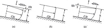
-
The maximum velocity is everywhere at the surface while the maximum shear rate is at the bed. The solution thus gives no support to the belief that the weight of the ice above squeezes out the underlying ice at a faster rate.
In other words, there was no suggestion of the brick-and- mortar action of free extrusion flow. Nye also assumed that isotropic stress (pressure) did not affect deformation rate, and noted that this was at odds with the assumption in Demorest’s extrusion flow concept.
Since 1951, advancements have been made in representing ice as a nonlinear fluid, and solving the equations of motion for all components of stress (full Stokes flow). Great progress has been made incorporating crystalline anisotropy into constitutive relations, and we now understand basal motion and sliding much better. Even the ‘grand unsolved problem’ (Reference WeertmanWeertman, 1976) of marine ice-sheet stability and sea-level rise is yielding to research. But that’s another story.
4. The Death of Free Extrusion Flow
4.1. The death scene
The death of the free extrusion-flow hypothesis came mercifully swiftly; the victim did not linger. In a letter to the Journal of Glaciology, Joel E. Reference FisherFisher (1952) objected to Reference NyeNye’s (1951) contention that extrusion flow seemed to be improbable. Fisher made the reasonable suggestion that deeper and older ice should be intrinsically softer, because impurities would have migrated to grain boundaries, where they could enhance the thickness of those intergranular water films by depressing the melting temperature, and facilitate grain-boundary sliding. However, it is clear that Fisher had missed Nye’s point that extrusion flow was mechanically unsound, because Fisher then went on to suggest that therefore the softer basal ice would produce extrusion flow.
In his reply, Reference NyeNye (1952b) reiterated that the major issue was not the constitutive properties of the ice, but rather the global imbalance of forces. To illustrate this point, he analyzed the forces acting horizontally on a section ABC (Fig. 12) of an idealized ice sheet resembling an east-west profile from the center of Greenland to the coast (a distance of approximately l in Fig. 12). The force per unit width on AC due to ice overburden pressure alone (see Equation (3a)) would be ρgz 2/2 directed toward the ice-sheet margin. An undercurrent of free extrusion flow would also produce an outward-directed force along AB, and that force would also tend to pull ABC outward toward the ice-sheet margin. The unbalanced pressure force on AC alone would accelerate the ice such that:
Balance (or imbalance) of forces in an idealized Greenland ice sheet. From Nye (1952b).

-
Starting from rest under this acceleration a particle of ice would move the distance AB in 2 hours. Or, if the acceleration were sustained for 100 years, which is not long compared with the lifetime of a piece of ice in Greenland, the ice would reach nearly one-fifth the velocity of light. (Reference NyeNye, 1952b, p. 53)
This simple illustration was powerful enough to suppress mention of free extrusion flow in polite glaciological circles for several decades. It was also ironic that the physically tenuous idea of free extrusion flow, for which Max Demorest achieved the greatest renown (or notoriety) among glaciologists, was ultimately destroyed by a speed-of-light argument that had much in common with his own argument (Reference DemorestDemorest, 1939) against von Engeln’s physically suspicious ideas about ice-flow waves and roches moutonnetes.
4.2. Death-cheating loopholes?
Nye concluded his 1952 letter by saying
-
I suppose that it might be possible to achieve the extrusion result with a sufficiently deep and narrow valley of the right shape, but I feel that anyone who wishes to make out a case for a theory of extrusion flow must first show that the proposed system is in statical equilibrium, and then that the forces required for this equilibrium can in fact be sustained by the ice.
So, could a hard-core extrusion advocate save the free extrusion-flow theory from oblivion by following the only path left open by Nye? Two ideas could be followed. First, can a valley support extrusion flow if it is deep enough and narrow enough? Second, can the forces on ABC in Figure 12 be balanced during extrusion flow in a way such that ice can survive mechanically?
4.2.1. Extrusion flow in deep narrow valleys?
Two factors must be considered to answer the first question. These are channel shape, and distribution of viscosity with depth. Shield volcanoes (e.g. Mauna Loa in Hawaii) extrude lavas with relatively low viscosity. After the upper free surface of a lava flow congeals, lava can be seen emerging from tunnels, and it flows fastest in the center of the tunnel. Similarly, if ice were to find itself in a large inclined rigid pipe with a rough surface at which the velocity goes to zero (Fig. 13a), then the fastest flow would be in the center, farthest from the walls, and a vertical profile would show extrusion flow.
Extrusion flow would occur in inclined closed pipes (a), but it does not occur in broad open channels such as (d). Where, in a succession of increasingly open channel shapes such as (b) and (c), does extrusion flow cease?

In order to get extrusion flow in an open channel, ice near the surface must, to some degree, act like the rigid top of the pipe by applying a restraining force. Suppose that ice fills a valley with overhanging walls. If the walls nearly meet at the top, i.e. have a separation small compared to the radius R of the channel (Fig. 13b), then the channel is open, but flow in it probably still closely resembles flow in a closed tube. Shear stresses in the narrow neck and under the overhang can impede the deeper ice enough to allow extrusion flow. Now we can imagine a sequence of valleys, with the overhang diminishing until the walls approach verticality (Fig. 13c), then adopt progressively lower slopes approaching a classic broad U-shaped glacial valley (Fig. 13d), in which extrusion flow does not occur. There must be a transition from extrusion flow to no extrusion flow somewhere in this sequence. The first part of the first question can be rephrased as: ‘Does that transitional shape ever occur naturally in valleys that contain ice?’
The second factor that can influence the answer to question 1 is the distribution of effective viscosity in the channel. For example, if the viscosity was very high near the surface and very low at greater depths, perhaps the upper ice could be held back by the upper walls due to its stiffness. Then it might act like the rigid top of the pipe in Figure 13a, allowing the softer lower ice to extrude.
Jérôme Léchot (unpublished information) adapted and used a finite-difference code written by Heinz Blatter and Andy Aschwanden to explore whether free extrusion flow could be possible in a deep and narrow, rectilinear, parabolic-shaped channel with a range of vertical distributions of effective ice viscosity. Because the model solved the momentum conservation equations, the forces were always balanced. Even for glaciers four times deeper than their surface width, with effective viscosities an order of magnitude greater at the surface than at the bed, no extrusion flow was found. These numerical experiments suggest that if extrusion flow can exist in deep narrow valleys over distances that are long relative to the channel cross-section dimensions, the necessary channel geometries and effective viscosity distributions are not found in nature.
4.2.2. Tension in Greenland?
To address Nye’s second question, extrusion-flow advocates might appeal one last time to the mortar-and-brick analogy, by asking whether a tensile force at AC in Figure 12 could pull the ice ‘brick’ to the left, to balance the shear force along AB (created by an extrusion undercurrent), which would pull the ice ‘brick’ to the right. The extrusion-flow advocates would first have to estimate the shear force along AB. Letting x and z be horizontal and vertical coordinates, they would realize that the net shear force (per unit width) is just the shear stress (per unit width) τ(x) integrated along AB. Demorest and other glaciologists of his era were aware that Reference DeeleyDeeley (1908) had estimated the viscosity of glacier ice to be μ =1.25 × 10¹³ Pas. The constitutive parameter μ relates shear stress in a linear viscous fluid to velocity gradient, as in Equation (7). Therefore, the extrusion-flow advocates would need only to estimate the reversed velocity gradient ∂u/∂z along AB. If they represented the ice thickness profile by H(x), and the net mass balance rate high on Greenland by ḃ (assumed to be uniform), mass conservation would produce the depth-averaged horizontal velocity

Because the ice is frozen to the bed, the depth-averaged velocity gradient is u s(x)/H(x), where u s(x) is the velocity at the ice-sheet surface. This gradient could be approximated with u(x)/H(x) (perhaps with a scaling factor of order unity). Now, assuming a typical extrusion-flow profile as in Figure 6c, it would not be unreasonable to approximate the magnitude of the reversed velocity gradient at depth z ≈ H/2 as one-tenth of the depth-averaged gradient, i.e.

The shear stress in the ice sheet along AB would then be

The extrusion advocates might also argue that the undercurrent is present only out to l/2where l is approximately the ice-sheet span in Figure 12. They might next assume for simplicity that H was also uniform out to l/2, so that the shear force (per unit width normal to the flow) on AB would be

(The second minus sign appears because the shear force acts on a downward-looking face.)
This force F AB must be balanced by a tensile force F AC =-σAC × H/2 acting in the negative x direction across AC, where -σ AC is the average tensile stress on AC. Then

With typical values for Greenland of ḃ ≈ 03 m a-1 (ice equivalent), H ≈ 3000 m, l ≈ 300 km, and Deeley’s viscosity estimate of μ ≈ 1.25 × 10¹³ Pas, Equation (14) produces a tensile stress (which is positive) of σac ≈ 107Pa, or 100bar, which is rather large. But the situation gets even worse for the extrusion supporters. The vertical stress σzz must still support the weight of the ice, so it must be compressive (less than zero) and its magnitude must be at or close to the overburden pressure ρgz. At depth z = H/2,

Ice responds to the differential stress (σ zz – σ AC), and since σ zz is compressive while σ AC is extensional, the differential stress could exceed 200 bar. Ice actually fails by plastic flow under tensile stresses of just a few bars, and fails by brittle fracture under tensile stresses of 10-20bar. Although the forces could be balanced, the upper layers of the ice sheet would have flowed or broken catastrophically long ago, and failed dismally to act like the rigid brick that squeezes out the mortar.
If this viscous-flow approximation seemed too complicated, extrusion advocates could have learned from Reference NyeNye (1951) that they could take a simpler alternative approach by assuming that ice is plastic. Basal shear stresses on many glaciers appear to fall in a narrow range around 105Pa, or 1 bar, so ice can be approximated as a plastic solid with a yield stress τ 0 of 1 bar. If we assume that the ice along AB in Figure 12 is yielding plastically in extrusion flow, then the shear stress -τ AB(x) in Equation (13) acting on the bottom side of the region ABC could be replaced with 105 Pa, or 1 bar. The force F AB in Equation (14) could be replaced by F ab = ‒τ0 l/2, and the tensile stress σ AC on AC needed to balance F AB would then be

which is similar to the approximation obtained from Equation (14) by assuming viscous flow. This is still an outrageous value of tensile stress, and one that ice cannot support. A death-cheating loophole just closed for free extrusion flow on ice sheets.
4.3. Messages from the depths
The definitive test of the extrusion flow theory was measurement of the deformation of vertical boreholes through glaciers. A casing left in a shallow borehole in Hintereisferner in 1901 by Blümcke and Hess (Reference Hess and GutenbergHess, 1933) was rediscovered in 1933, and found to have developed a forward slant, implying that the velocity was greatest at the surface (Reference Matthes and MeinzerMatthes, 1942).
The Jungfraujoch Research Party from Cambridge drilled a borehole that reached close to bedrock in the Jungfraufirn (Reference PerutzPerutz, 1950; Reference Gerrard, Perutz and RochGerrard and others, 1952). Figure 14 shows how its shape changed over a period of 2 years. There was no indication of extrusion flow.
Deformation measured over the course of 2 years in the Jungfraufirn borehole. From Reference PerutzPerutz (1953). Reproduced with permission of Nature Publishing Group.

Rudolf Reference Streiff-BeckerStreiff-Becker (1953) suggested that the Jungfraufirn borehole may have failed to detect extrusion flow simply because it had been drilled in the wrong section of the glacier. The hole had been drilled at 3350m elevation, where the glacier was thin and the mean annual air temperature was cold. He suggested that these factors combined to prevent the basal ice from getting warm enough to undergo extrusion flow, and he predicted that, if another hole were to be drilled where the surface was a few hundred meters lower, then warmer and more plastic lower layers would be found. He was correct in that assertion, but, like Fisher, he had not fully appreciated that the problem was the improbability of creating the force patterns necessary to drive extrusion flow, not the constitutive properties of the ice. In the rare cases where the force patterns could be created, and where transient and local extrusion flow has been seen (e.g. Reference Hooke, Holmlund and IversonHooke and others, 1987), the conditions were as Streiff-Becker described, with a cold stiff ice lid on top of warm soft ice.
Over the next two decades, other holes were drilled in the North American glaciers Malaspina Glacier (Reference SharpSharp, 1953), Salmon Glacier (Reference MathewsMathews, 1959), Saskatchewan Glacier (Reference MeierMeier, 1960), Blue Glacier (Reference Shreve and SharpShreve and Sharp, 1970) and Athabasca Glacier (Reference RaymondRaymond, 1971), and in other locations as well. In virtually all cases, the basal ice was at the pressure-melting temperature, yet all holes gave the same result: the horizontal velocity decreased with depth. The free extrusion flow theory was dead.
5. The Afterlife
Two other types of ‘extrusion flow’ were presented at various times to support the free-extrusion flow hypothesis, even though now we can see that the controlling physics had significant differences. I suggest that those analogies were actually inappropriate. Because the death of free extrusion flow had been so sudden and so decisive, these other types of flow received little attention for decades. Perhaps glaciologists were a little bit gun-shy.
In capped extrusion flow, the upper layers of ice are actually able to exert a restraining force sufficient to balance the shear force associated with extrusion flow. In rotational flow, deeper layers may move faster than layers above, but the motion is a rigid body rotation rather than a deformation, so in a sense ice is not really ‘extruded’ at all.
5.1. Capped extrusion flow
Over short distances, longitudinal stress gradients can prevent shallow ice layers from being carried along by faster-moving ice below, and extrusion flow can be supported locally. The importance of relatively short scale lengths was not always appreciated during the debate about free extrusion flow.
5.1.1. Extrusion of soft basal ice
Hans Carol was a Swiss mountaineer and glaciologist who was curious about the formation process of roches moutonnées. Through crevasses and tunnels, he was able to get 50 m below the surface of Upper Grindelwald Glacier (Oberer Grindelwaldgletscher) to observe the ice as it moved past a bedrock bump (Reference CarolCarol, 1947). He found that as ice approached the bump, it appeared to undergo some degree of pressure melting on grain boundaries (see shaded area in Fig. 15a). As a result, this ice was less able to tightly hold the clasts that were abrading the bedrock. From this, he inferred that the erosion rate was lower on the upstream side of the bump than on the area farther upstream, and the bump could be a self-sustaining feature of the bedrock.
(a) Ice flow and erosion on a bedrock protuberance. Increased pressure in the hatched zone produces partial melting on grain boundaries, softer ice, and reduced drag force and frictional resistance on the clast. With reduced erosion on the upstream side of a bump, the bump can grow. (b) Measured daily displacements in the softened ice and in the hard ice above it. The soft basal layer accelerates through the narrow gap over the top of the bump. Adapted from Reference CarolCarol (1947).

Carol also measured the rates of displacement of the ice at several levels on the upstream side of the bump (Fig. 15b), and found that the softened basal ice moved nearly twice as fast as the harder overlying ice. At the length scale of the bump, the upper ice was rigid enough to resist being accelerated to match the fast flow below.
Although Carol did not cite Demorest’s or Streiff-Becker’s extrusion flow, the editors of the Journal of Glaciology (chief editor Gerald Seligman) did make the connection, and added a note preceding Carol’s paper:
-
(This paper in addition to its main theme gives observational evidence of plasticity and faster flow in the lower strata of a glacier under pressure. The conditions it describes provide additional support for the Extrusion Flow hypothesis. Ed.)
5.1.2. Extrusion transverse to valley axis
Charlie Reference RaymondRaymond (1971) drilled five holes in a line across Athabasca Glacier, Alberta, Canada, and monitored the subsequent changes in inclination of the holes. The velocity components along the valley axis profiles decreased continuously with depth as expected; however, Figure 16 shows that in some places, flow transverse to the valley axis was greater in magnitude at depth than at the surface. Raymond explained that this pattern was a direct consequence of continuity in any cross section with a concave bed profile, a convex transverse surface profile that drives flow toward the margins, and plug-like compressing longitudinal motion due largely to basal sliding that is uniform across the channel.
Flow in a transverse section in the ablation area of Athabasca Glacier. From 1A to 5A, the lateral flow is greater at depth than at the surface. From Reference RaymondRaymond (1971).

-
Although extrusion flow has been discredited as a mechanism for the longitudinal component of flow, it may represent the normal pattern of transverse flow associated with the convex lateral surface profile in the ablation area of valley glaciers.
Raymond also pointed out that the restraining force on the upper layers (which was absent in Demorest’s free extrusion flow;section 4.2), is provided here by the valley walls. He also noted that in accumulation areas with concave transverse surface profiles, flow inward toward the channel center should similarly be faster at depth than at the surface (i.e. roughly reversing the directions on all the vectors in Figure 16).
5.1.3. Transient longitudinal extrusion flow
In 1984, Roger Reference Hooke, Holmlund and IversonHooke and others (1987) measured inclination at five times separated by 1-3 weeks in a borehole near the top of a riegel in Storgläciaren, Sweden. During July, ice near the bottom of the hole moved several times faster than ice near the surface (Fig. 17). The azimuth of motion was nearly 50° to the right of the surface flow, and directed toward an overdeepening in the bed downstream from the hole. Hooke and his co-authors were hesitant to use the term ‘extrusion flow’ to describe the July pattern, which resembled Demorest’s discredited longitudinal extrusion flow.
Velocity magnitude and azimuth in a hole at Storglaciären. During July, basal flow was several times faster than surface flow, and directed up to 50º to the right, down the basal slope. During August neither the magnitude nor the azimuth varied significantly with depth. From Reference Hooke, Holmlund and IversonHooke and others (1987).

-
The term ‘extrusion flow’ was apparently first used by Demorest (1941, 1942), who suggested that ice became more plastic with depth and might therefore flow faster. Reference NyeNye (1952a) showed that such flow was impossible under normal circumstances, in which the glacier is wide and bed irregularities small compared with the ice thickness. This is because a surface layer of ice that was being dragged outward by shear stresses exerted on its bottom by faster moving deeper ice as well as pushed outward by imbalanced hydrostatic forces resulting from the down-glacier surface slope would not be in static equilibrium. The term has thus vanished from the literature, for the most part, and we reintroduce it with some reluctance. However, we have measured flow similar to that originally hypothesized by Demorest and, rather than coin a new term to describe it, we have chosen to resurrect the old term, with the understanding that all available evidence suggests that such flow is only possible in situations where a special valley geometry and perhaps temperature regime result in static equilibrium of the surface layer, despite the additional down- glacier shear force on its bottom.
Reference Hooke, Holmlund and IversonHooke and others (1987) suggested that the extrusion flow occurred when transient high water pressure locally decoupled the ice from the bed, removing a restraining basal shear force. Storglaciären is polythermal, and the cold and stiff upper ice was probably sufficiently rigid to bridge across the faster-moving lower ice, providing the cap. Rudolf Reference Streiff-BeckerStreiff-Becker (1953) had argued for extrusion flow under these conditions, although he had not fully appreciated the importance of the restraining cap (see section 4.3). In August, the flow in the deep ice changed: it aligned with the flow in the ice above in both magnitude and direction (Fig. 17). Reference Hooke, Holmlund and IversonHooke and others (1987) attributed this change to decreasing basal water pressure, which allowed the ice to recouple to the bed, eliminating the extrusion flow.
Subsequent observations at other glaciers have confirmed the possibility of faster flow at depth when water decouples the ice from the bed. Luke Reference Copland, Harbor, Minner and SharpCopland and others (1997) measured a tilt profile at Haut Glacier d’Arolla, Switzerland, that was suggestive of local extrusion flow, but they were unable to exclude instrumental uncertainties. Using a threedimensional flow model developed by Reference BlatterHeinz Blatter (1995), Reference Hubbard, Blatter, Nienow, Mairand and HubbardAlun Hubbard and others (1998) showed that for an imposed basal velocity pattern typical of this glacier, the basal ice could uncouple mechanically from the bedrock in the region where the extrusion flow may have occurred. Hilmar Reference Gudmundsson, Bauder, Luthi, Fischer and FunkGudmundsson and others (1999) saw a reversal in tilt rate for over 1 month at Unteraargletscher. While they could not completely exclude relative motion between the tilt sensor and the ice, the sense of tilting indicated a reversed velocity gradient and local extrusion flow, and the timing in summer corresponded to the time when basal decoupling would be most likely to occur.
5.1.4. Flow over a wavy bed
When ice slides uniformly over a bed with undulations whose wavelength λ is short relative to the ice thickness, flow in the basal layers is affected by those undulations to a far greater extent than flow in the upper layers. Incompressibility suggests that basal ice, trapped between the bed and the insensitive upper layers of the glacier, should compress vertically and extend longitudinally to get over bumps, and it should extend vertically and compress longitudinally when passing over troughs. That horizontal extension and contraction produces acceleration over the upslopes, and deceleration over the downslopes. Numerical studies have shown that in some conditions, these velocity effects can reverse the normal vertical gradients of velocity, creating local extrusion flows. For example, Reference GudmundssonHilmar Gudmundsson (1997a) derived analytical perturbation solutions for flow of a constant-viscosity material over an inclined frictionless wavy bed. Velocities were nondimensionalized with the sliding speed, and both distance X and height Z were nondimensionalized with bed wavenumber 2π/λ. Figure 18 shows contours of VX, the component of velocity directed parallel to the mean bed above one cycle of a sine wave in a glacier bed. For this particular combination of bed shape and ice thickness, a maximum in velocity VX occurs approximately 1/2π wavelengths above the peak, and over the trough a maximum in VX can be seen right at the bed. However, these inverted velocity gradients have very limited spatial extent (a fraction of a wavelength), and the restraining force is provided by the overlying ice in which longitudinal stress gradients resist faster flow.
Contours of nondimensional horizontal velocity VX when ice slides over a sinusoidal bed. Curve below the graph indicates amplitude and phasing of one wavelength λ of the bed. The ratio of bed amplitude to wavelength is 0.1/(2π)≈0.016, and the ratio of wavelength to ice thickness is 0.2π≈0.6. Both distance X and height Z have been nondimensionalized with bed wavenumber 2π/λ. V x has a maximum above the bed peak and minimum over bed trough at 1.5. Adapted from Reference GudmundssonGudmundsson (1997a). Sine wave added by E.D.W.

In a companion paper, Reference GudmundssonGudmundsson (1997b) used a full- stress finite-element model to show that localized capped extrusion flow could be even more pronounced for a power- law fluid sliding over a strongly undulating bed with amplitude too large to be addressed with his analytical perturbation treatment.
5.2. Rotational flow
Because of the interest in extrusion flow stimulated by work by Streiff-Becker and Demorest, other authors pointed out situations where deeper ice flowed faster. In some cases, the flow resembled a rigid-body rotation rather than extrusion. When a body moves by rigid rotation, cohesive forces within the ice prevent strain; equilibrium requires a balance of torques. This section addresses this third type of ‘extrusion’, i.e. rotational flow.
Charlie Raymond has pointed out (personal communication, 2010) that wherever a glacier surface S(x) is concave in the longitudinal profile, ice at depth can move faster than ice at the surface. The upper surface of a glacier is traction-free, so a pole installed normal to the surface stays normal to the surface, and the bottom of the pole must move faster than the top by rotation as the pole moves through the decreasing surface gradient. The increase in this rotational flow u r with depth (h-z) is proportional to the flow velocity u s at the surface, and the surface curvature, i.e.

The decrease in velocity with depth due to shearing flow can be estimated from Equation (1):

The velocity is maximum at the depth where their sum is zero, i.e. at

For example, for a glacier that is 100 m thick, with surface slope changing by 10° in 400 m, and basal sliding accounting for half the surface motion, Equation (20) puts the velocity maximum at ~30 m depth. If 90% of the surface motion was due to basal sliding, then the velocity maximum would be at 50 m depth.
George Gibson and James Dyson (Reference Gibson and DysonGibson and Dyson, 1939) observed wedge-shaped annual layers separated by summer dirt layers in Grinnell Glacier, a small cirque glacier in Montana. They presented the analogue rotational flow model illustrated in Figure 19. Each wedge-shaped shingle represented 1 year’s accumulation in the accumulation area. Every year, another shingle would be added to the stack, and the stack would be pushed down by a corresponding amount. If the thin ends of the shingles could be ablated below the equilibrium line (at the apex of the top shingle), the surface profile and the internal stratigraphy would closely approximate the structures seen at Grinnell Glacier. The shingles slide a small amount relative to one another as they adjust to the bed slope, but the model assumes that virtually all of the motion is due to sliding over the substrate, i.e. the velocity maximum (Equation (19)) is at the bed.
A stack of tapered shingles provides an analogue for rotational flow in a cirque glacier. The thick ends of the shingles slide on the curved surface without deformation. Each shingle represents 1 year’s net accumulation. Adapted from Reference Gibson and DysonGibson and Dyson (1939). Reproduced with permission of Geological Society of America. Glacier profile overlay added by E.D.W.

Other observers, including Louis Agassiz, had noted that, high on a glacier, the annual layers dipped downstream, but as he followed the glacier downstream, the dip of the annual layers diminished, and in the ablation area the layers could even dip upstream. In 1847 (Nouvelles études, p. 170) Agassiz speculated that this pattern required the deeper ice (corresponding to the thicker ends of the shingles in Fig. 19) to move faster. Rudolf Streiff-Becker (Fig. 6) saw the same pattern of tilting stratigraphy, and like Agassiz he thought that extrusion flow was necessary to account for the pattern. Neither Agassiz nor Streiff-Becker recognized that if shear flow along the layer interfaces was added, stratigraphy with a similar qualitative pattern of dips would still result, but without the need to invoke faster motion at the bed. In small cirque glaciers where the stresses are low enough that ice can act like a rigid body, rotational flow as in Figure 19 is largely sufficient to produce the observed layer-tilt pattern. However, purely rotational flow is not always necessary to produce observed patterns of layer dip in larger or more dynamic glaciers.
W. Vaughan Lewis was a lecturer in geography at Cambridge, where he studied shoreline processes and glacier flow, and mentored younger glaciologists such as W.H. Ward, John Glen and John Nye in field programs on Norwegian glaciers (Reference Manley and WardManley and Ward, 1961). In 1949, he analyzed the motion of several Norwegian cirque glaciers in terms of rotational slip along a basal surface (as in Fig. 19), combined with rotational slip along a large number of curved internal failure surfaces that could be seen where they exited the glacier in the ablation area. Reference LewisLewis (1949) found an association between these slip surfaces and foliation surfaces (Forbes’ ‘veined structure’) in which the c-axes of ice crystals were aligned normal to the slip surface, allowing easy glide. Lewis built a mechanical analogue ‘computing device’ (Fig. 20) into which he could measure the gravitational torque on crescents of plywood scaled to represent possible failure surfaces within cirque glaciers. Knowing the appropriate scaling parameters, he could then find the gravitational torque (per unit width) on the corresponding surface within the glacier. Assuming a yield stress of approximately 105 Pa (1 bar), he could calculate whether that gravitational torque could be supported along the surface within the ice, or whether it would fail as a slip surface.
Analogue device used by Lewis to compute torques along possible slip surfaces within cirque glaciers. From Reference LewisLewis (1949). Reproduced with permission of Wiley–Blackwell.

In discussing the significance of rotational flow for erosion of cirque floors, Lewis compared his ideas to the Demorest extrusion-flow theory. His thoughts in some ways presaged Reference NyeJohn Nye’s (1952b) reply to Joel Fisher. After pointing out that glacier ice does not actually get softer under pressure, Lewis noted that
-
There is another more fatal weakness to the theory of extrusion flow as usually presented, and that is that it assumes that in basins the deep ice moves quicker than the overlying, supposedly more rigid, ice. Why, except possibly in extremely deep and narrow glacial valleys or valleys with constrictions, the overlying ice is not carried forward by the quicker moving underlying ice is not explained.
He also noted that rotational slip could account for the patterns of layer tilt reported by Streiff-Becker (e.g. see Fig. 6) as easily as extrusion flow could.
John Gill McCall was an American paratrooper in World War II, and a skilled mountain climber. He earned a PhD at Cambridge, UK, in 1953, then took up a professorship at the University of Alaska, where he was very active until his very promising career was cut short: he died of poliomyelitis in 1954 at age 31 (BGS, 1955). In his PhD research on the Norwegian cirque glaciers (Reference McCallMcCall, 1952) he called into question whether discrete shear bands existed, or whether differential rotational flow was distributed throughout the depth. Jean M. Clark and W. Vaughan Lewis (Reference Clark and LewisClark and Lewis, 1951) noted the connection between their rotational flow concepts in cirque glaciers, and Reference NyeNye’s (1951) plastic slip-line fields. Rather than being a distinct phenomenon, extrusion flow by rotational slip appeared to be merging back into the continuum of general glacier flow governed by the same conservation and constitutive laws. In small cirque glaciers, stresses could be too small to cause significant internal deformation, but large enough to cause basal slip. For larger cirque glaciers, the expectation of faster flow at depth diminished with the realization that distributed internal shear strain along rotational surfaces (or slip lines) could preserve the pattern of tilted layers without requiring faster flow at depth.
6. Conclusions
6.1. Role of Journal of Glaciology
The British Glaciological Society, founding publisher of the Journal of Glaciology, was apparently a vigorous presence in the Cambridge scientific lecture and meeting scene of the late 1940s. As a new journal in 1947, the Journal of Glaciology welcomed contributions on all aspects of ice in the environment, and its editor, Gerald Seligman, effectively engaged specialists from outside the traditional geology or glaciology communities. These factors created an environment in which vigorous debate and innovation could thrive. When the Journal began publication in 1947, extrusion flow had been championed in various forms for over 100 years. However, the Journal published papers questioning traditional views, while also publishing new approaches to glacier flow theory from young scientists. It also published the comments and debates at the meetings where these new ideas were discussed and debated. I think that this open approach contributed substantially to the rapid resolution of the free extrusion-flow debate. As a result, the key papers in the debate were published in the Journal of Glaciology. Following the sudden demise of free extrusion flow in the pages of the Journal in 1952, readers have seen articles describing capped extrusion flow and its connections with a currently important research area, basal processes and basal motion.
After exclusion of books, theses and articles published before the Journal of Glaciology began publishing in 1947, this article contains 55 references. While recognizing that this may be a biased sample, I find that 33 were published in the Journal of Glaciology and 2 more in Annals of Glaciology, accounting for nearly two-thirds of these publications.
The first editor, Gerald Seligman, was deeply interested in the history of glacier flow (e.g. Reference SeligmanSeligman, 1947, 1949). For several decades, the Journal helped its readers to understand our history by publishing its ‘Early Discoverer’ series. More recently, that service has been taken over by occasional retrospective issues such as the 1987 Special Issue commemorating the 50th anniversary of the founding of the British Glaciological Society, and this one, 56(200), commemorating successful uninterrupted publication of 200 issues. As a member-supported publication of the International Glaciological Society, the Journal of Glaciology continues to serve glaciologists studying all corners of the cryosphere.
6.2. Lessons for the future
Max Demorest tried to bridge the gulf between the two solitudes, by bringing mechanics to bear on previously nonquantitative geological and glaciological questions. Sometimes he succeeded, but sometimes, as with free extrusion flow, he failed. In the past 50 years, more young glaciologists have been able to straddle that gulf between taxonomy and physics, or between description and process studies. As a result, the field of glaciology has grown and progressed substantially, to the point where it is now a large discipline with its own sections within the American Geophysical Union and European Geosciences Union. While glaciology is a rapidly growing field in this era of climate change, we should recall how small our field has been through its history. Louis Agassiz (the ultimate taxonomist?) may be better known for his classification of fossil fishes than for his work on glaciers. Richard M. Deeley may have a larger following among antique train hobbyists than among glaciologists, and Max Demorest may be known to more World War II history buffs than glaciologists.
I hope that this narrative offers another sobering caution to modern glaciologists. We must recognize the ease with which otherwise accomplished scientists can mislead themselves in their thinking by holding too tightly to an incorrect idea. For Louis Agassiz, it was the idea that glaciers moved by dilatation. For Max Demorest, it was the idea that motion in ice-sheet interiors was governed by different physics from flow in valley glaciers. For Rudolf Streiff-Becker, it was the idea that Claridenfirn was only 110m deep at his upper marker. The message to us all, as expressed by Thomas E. Reference KidaKida (2006), should be ‘Don’t believe everything you think.’
Acknowledgements
Thanks to Garry Clarke, editor for this special issue of Journal of Glaciology, for suggesting this topic, which I had previously explored while a PhD student at the University of British Columbia. Ralf Greve, as scientific editor, also provided helpful suggestions. I am grateful to Charlie Raymond for illuminating discussions about flow in Athabasca Glacier, and to Al Rasmussen for discussions about mass balance in connection with Claridenfirn. Bernard Hallet offered helpful insights about Stokes flow around basal clasts, and pointed out the observations by Hans Carol. I am particularly indebted to Heinz Blatter for carefully reviewing the manuscript, and for sharing current work at ETH on flow in deep narrow channels, for providing background information on Claridenfirn, and for translating passages that have greatly helped me to form a more rounded perspective of Rudolf Streiff-Becker, most of whose research was published in German.



