





1 Introduction
1.1 Bulk scaling for the CUE
Dyson’s circular unitary ensemble (CUE) [Reference Dyson22] is identical to the set of
$N \times N$
 matrices from the classical unitary group chosen with Haar measure. From the latter viewpoint, which has its origins in the work of Hurwitz (see the review [Reference Diaconis and Forrester20]), it is a classical result of Weyl [Reference Weyl71] that the corresponding eigenvalue probability density function (PDF) is given by

From this starting point, Dyson [Reference Dyson23] deduced that the general n-point correlation function

has the determinantal form

where

Dyson also considered the bulk scaled
$N \to \infty $
 limit, in which the angles are scaled
$\theta _l = 2 \pi X_l/N$
 so that in the variables
$\{X_l\}$
 the mean eigenvalue density is unity, with the result

where

Our interest in the present paper relates to the structure of the large N expansion of the bulk scaled n-point correlation, which is the function of
$\{X_l\}$
 and N in the second expression in (1.5). Beyond the CUE, we take up this question for the class of circular
$\beta $
 -ensembles specified by the eigenvalue PDF

where

Note that the CUE is the case
$\beta = 2$
 of (1.7). For a construction of Hessenberg unitary matrices which realise (1.7) for general
$\beta> 0$
 , and moreover show that the bulk scaled limit is well defined, see [Reference Killip and Nenciu54].
In the case of the CUE, due to (1.3), the question of the structure of the large N expansion of the bulk scaled k-point correlation function reduces to the simple question of expanding for large N

A significant feature is that in this functional form N need not be restricted to positive integer values, but rather may be regarded as a continuous parameter. Adopting this viewpoint, one sees that it is an even function of N (as well as in
$(X-Y)$
 ), possessing an expansion in powers of
$1/N^2$


In particular, for the bulk scaled two-point correlation function, this implies that for large N

a result which has application in interpreting data for the two-point correlation function of the Riemann zeros at large height [Reference Bogomolny, Bohigas, Leboeuf and Monastra4, Reference Forrester and Mays35, Reference Bornemann, Forrester and Mays14]. More on the consequences of our results in relation to structure seen in particular empirical distributions for the Riemann zeros at large height is to come later in this article. At present the main point to be emphasised is that the asymptotic expansion of the general k-point correlation function, to all orders in
$1/N$
 , contains only powers of
$1/N^2$
 ,

for some
$\{ \rho _{(n),l,\beta = 2}^{\mathrm {bulk}}(X_1,\dots ,X_n) \}$
 .
Establishing such a result has consequences for the large N expansion of the probability density function of the distribution function for the spacing between a given eigenvalue and its l-th neighbour to the right. These distribution functions are fully determined by the probabilities
$\{ E_N(k;(0,\phi )) \}_{k=0}^N$
 for the interval
$(0,\phi )$
 containing exactly k eigenvalues, which in turn have for their generating function the expansion

valid for any one-dimensional point process
$(\cdot )$
 on the circle (see, e.g., [Reference Forrester29, §8.1] in relation to the above theory). Thus, specialising to the case of the CUE, it follows by substituting (1.12) in (1.13) that for large N

for some
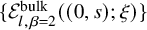
$\{\mathcal E^{\mathrm {bulk}}_{l,\beta = 2}((0,s);\xi ) \}$
 (convergence of the implied infinite sums at each order which form the
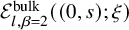
$\mathcal E^{\mathrm { bulk}}_{l,\beta = 2}((0,s);\xi )$
 can readily be established; see [Reference Bornemann, Forrester and Mays14, Lemma 2.1]). In fact one has available the explicit small-s expansion ([Reference Tracy and Widom70], [29, Eq. (8.79), extended to two further terms according to the methodology therein])

which is immediately observed to permit an expansion in
$1/N^2$
 to each order in s exhibited. In keeping with the text below (1.11), one remarks that computable functional forms of the term at order
$1/N^2$
 for the distribution of the spacing between eigenvalues, and this distribution after a thinning of the eigenvalue sequence (since [Reference Bohigas and Pato5] it is known that the latter is controlled by the parameter
$\xi $
 ), both of which relate to
$\mathcal E^{\mathrm {bulk}}_{l,\beta = 2}((0,s);\xi ) |_{l=1}$
 , have been used in [Reference Forrester and Mays35, Reference Bornemann, Forrester and Mays14] for purposes of interpreting empirically determined spacing distributions for the Riemann zeros at large height. A major finding of the present work in this regard – see Proposition 2.1 – is that correction at order
$1/N^2$
 is simply related to the leading distribution by a derivative operation.
1.2 Relationship to earlier work
Prominence to the structure of the large N asymptotic expansion of quantities in random matrix theory comes from several sources. The first, and probably the best known, relates to the
$1/N$
 expansion associated with the so-called loop equations [Reference Migdal60]. In this formalism the connected correlators for the product of linear statistics

each of which can be considered as the generating function for products of s monomials, are by an hypothesis on the existence of the
$1/N$
 expansion (this hypothesis has subsequently been proved in a number of prominent settings [Reference Borot and Guionnet16]) in the so-called global scaling limit fully determined by a triangular system of equations. As a concrete example, consider following [Reference Brini, Mariño and Stevan17, Reference Mironov, Morozov, Popolitov and Shakirov61, Reference Witte and Forrester75] a loop equation analysis applied to the Gaussian
$\beta $
 ensemble characterised by the eigenvalue PDF proportional to

(specifically here the N-dependent factor in the Gaussian implies the limiting density is supported on a compact interval,
$(-1,1)$
 to be precise, which is the requirement of global scaling). In relation to the averaged monomials
$\tilde {m}_k^{\mathrm {G}}(\beta ,N) := N^{-k/2-1} \langle \sum _{l=1}^N \lambda _l^k \rangle $
 , where the average is with respect to (1.17), the
$1/N$
 expansion in fact terminates at order
$N^{-k/2}$
 . As explicit examples, taking into account that by symmetry all the odd moments vanish, for the second and fourth moments one can calculate that (see, e.g., [Reference Dumitriu and Edelmann21])

where
$\tau :=\beta /2$
 . It is furthermore true that the moments satisfy the duality relation [Reference Dumitriu and Edelmann21]

(As in (1.9), although now for a different reason, namely that the quantities in question are polynomials in all parameters, both sides of (1.19) have meaning for continuous N.) In particular, the duality relation implies that for
$\beta = 2$
 the moments are even in N and so have an expansion in terms of
$1/N^2$
 ; for
$\beta \ne 2$
 the explicit results of (1.18) exhibit a
$1/N$
 expansion.
At the edge of the spectrum the Gaussian
$\beta $
 -ensemble permits a soft edge scaling [Reference Forrester27]

to a well defined statistical state with the eigenvalues spaced at order unity apart. Recent work of Bornemann [Reference Bornemann11, Reference Bornemann12, Reference Bornemann13] has for
$\beta = 1,2$
 and 4 established an asymptotic expansion of the density and the spacing distribution in powers of
$(N')^{-2/3}$
 ,
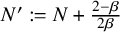
$N' := N + {2 - \beta \over 2 \beta }$
 , with moreover functional forms in the corrections relating to the limiting functional form by certain derivative operations, multiplied by a polynomial.Footnote
1
For example, in the case
$\beta =2$
 , when (1.17) corresponds to the Gaussian unitary ensemble GUE
${}^*$
 – here the asterisk indicates the use of global scaling with the limiting density supported on
$(-1,1)$
 – one has [Reference Bornemann11, Th. 2.1 in the case
$\xi =1$
 ] (extended to general
$\xi $
 in [Reference Bornemann13])

In [Reference Forrester and Trinh41], in relation to the spectral density for the Gaussian
$\beta $
 ensemble with
$\beta $
 even, it was established that the leading correction to the limiting density occurs at order
$(N')^{-2/3}$
 . Strictly speaking, the result was stated in terms of an N dependent shift in t, which is equivalent to the stated
$\beta $
 dependent shift in the meaning of
$N'$
 up to this order; on this point in relation to the cases
$\beta =1$
 and 2, see also [Reference Johnstone and Ma51]. One remarks too that the expansion (1.21), but with a weaker error bound, and a more complicated (but still computable) functional form of the
$N^{-2/3}$
 term was given in [Reference Forrester and Trinh40].
In the case of the Laguerre
$\beta $
 -ensemble, specified by the eigenvalue PDF proportional to

the works of Bornemann [Reference Bornemann11, Reference Bornemann12] establish an analogous result at the soft edge (scaled neighbourhood of the largest eigenvalue) for
$\beta = 1,2$
 and 4, although the parameter playing the role of
$N'$
 is now more complicated and depends on a (in relation to the expansion parameter for
$\beta =1$
 see too [Reference Ma57]), and the details of the polynomials in the functional forms of the expansion coefficients differ from those of the Gaussian case. At the hard edge, which is obtained by the scaling
$\lambda _l \mapsto x_l/4N$
 , a recent result from [Reference Forrester33] gives that particular gap probabilities permit expansion in powers of
$N_{\mathrm {L}}^{-2}$
 , where
$N_{\mathrm {L}} := N + a/\beta $
 , although no results were obtained in relation to the functional form of the coefficients. To leading order, this result was first established in the earlier work [Reference Forrester and Trinh42], which also contains computation of the functional form of some corrections; in relation to the leading order correction at the hard edge with
$\beta =2$
 we reference too [Reference Edelman, Guionnet and Péché24, Reference Bornemann8, Reference Perret and Schehr66, Reference Hachem, Hardy and Najim48]. Analogous results are also known at the hard edge of the Jacobi
$\beta $
 ensemble (see [Reference Forrester33, Prop. 4.6 and Remark 4.3.1], [Reference Forrester, Li and Trinh34, Appendix A of arXiv version], [Reference Winn74] for results relating to general
$\beta $
 , and [Reference Moreno-Pozas, Morales-Jimenez and McKay62] in relation to
$\beta = 2$
 . After hard edge scaling the correlations and spacing distributions no longer depend on N, but do depend on the Laguerre parameter, a say. Asymptotic expansions with respect to a and the re-centering of the position variables in relation to the hard edge to soft edge transition are of interest in the context of the length of the longest increasing subsequence problem [Reference Borodin and Forrester15]. Results on the optimal expansion parameter and the resulting functional forms are given in [Reference Baik and Jenkins3, Reference Forrester and Mays36, Reference Bornemann9, Reference Bornemann10].
The expansion in powers of
$1/N$
 for the bulk scaled correlation functions about
$\theta _l = 0$
 of the circular Jacobi ensemble, specified by the eigenvalue PDF proportional to

has been considered in the work [Reference Forrester, Li and Trinh34]. There, it was established for
$\beta = 1, 2$
 and 4 in the case of the general k-point correlation function, and for
$\beta $
 even in the case of the density that in the variable
$N_{\mathrm {cJ}} := N + p$
 the leading correction is proportional to
$N_{\mathrm {cJ}}^{-2}$
 .
1.3 Summary of results
In Section 2 the asymptotic expansion of the bulk scaled spacing distribution generating function
$\mathcal P_N^{\mathrm {CUE}}(2 \pi s/N;\xi )$
 as defined by (2.1) is established to be in powers of
$N^{-2}$
 to all orders; see (2.3). With the leading term denoted
$\mathcal P_{0,\beta = 2}^{\mathrm {bulk}}(s;\xi )$
 , and the first correction equal to
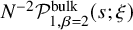
$N^{-2} \mathcal P_{1,\beta = 2}^{\mathrm {bulk}}(s;\xi ) $
 , the functional form
$\mathcal P_{1,\beta = 2}^{\mathrm {bulk}}(s;\xi )$
 is shown, using a
$\sigma $
 -Painlevé V characterisation, to be related to
$\mathcal P_{0,\beta = 2}^{\mathrm {bulk}}(s;\xi )$
 by the simple differential relation (2.8). The consequence of this result in the context of the empirical Riemann zeros spacing distribution at large height, and that of their thinning, is noted in item 2 of Remark 2.1. In Section 3 the explicit form of the
$2 \times 2$
 matrix correlation kernel specifying the Pfaffian point process form of the
$\beta = 1$
 and 4 cases of the circular
$\beta $
 ensemble is used to deduce that the large N expansion of the general n-point correlations are in powers of
$1/N^2$
 . This is the analogue of the CUE result (1.12), following from an expansion of the (scalar) correlation kernel, and lifts too to imply an analogous asymptotic expansion of the spacing distribution generating functions. Moreover, the first correction in the asymptotic expansion is shown, again using
$\sigma $
 -Painlevé characterisations, to be related to the leading term by a simple differential relation ((3.6) in the case
$\beta =1$
 and (3.12) in the case
$\beta =4$
 ). Also considered is the large N expansion of the structure function (this is essentially the Fourier transform of the truncated two-point correlation function). Proposition 3.4 establishes an asymptotic expansion in powers of
$N^{-2}$
 , and in (3.29) differential identities are given relating the first and second corrections to the limiting functional form. Section 4 makes use of known expressions in terms of generalised hypergeometric functions based on Jack polynomials (see, e.g., [Reference Forrester29, Ch. 13]) to establish that each n-point correlation with
$\beta $
 even is an even function of N. For the two-point function in this setting, an asymptotic expansion in inverse powers of N can be established, which must therefore only involve even powers. In addition, it is shown that the leading correction in the case of the two-point correlation function is related to the limiting functional form via a simple differential identity of the form already established for
$\beta =1,2$
 and 4. A recursion identity for multiple integrals, relevant to expressing higher order corrections in the
$1/N^2$
 expansion of the two-point correlation for the
$\beta $
 even circular ensemble to derivative operations of the limiting functional form, is given in Appendix A. Appendix B relates to the functional form of
$\xi ^k$
 in (1.13) for the circular
$\beta $
 ensemble with bulk scaling variables as in (1.14), to leading order in s but with N general. This allows for determination of the respective terms in the
$\beta $
 generalisation of the power series expansion (1.15), and thus provides data on the relation of the
$1/N^2$
 and
$1/N^4$
 corrections in relation to the limiting values.
2 Bulk scaled spacing distribution for
$\beta =2$


Let
$p_N^{(\cdot )}(k;x)$
 denote the probability that in the ensemble
$(\cdot )$
 , given there is an eigenvalue at the origin, there is an eigenvalue at x with exactly k eigenvalues in between. Suppose that
$(\cdot )$
 is rotationally invariant and has been bulk scaled so that the eigenvalue density is unity. Analogous to (1.13) we have the generating function expansionFootnote
2

which moreover is related to (1.13) by

where again bulk scaling (with eigenvalue density unity) is assumed.
It follows from the second expression in (2.1) and the
$1/N^2$
 expansion of the correlation functions that the bulk scaled generating function
$(2 \pi /N)^2 \mathcal P_N^{\mathrm {CUE}}(2 \pi s/N;\xi )$
 for large N, as for
$\mathcal E_N^{\mathrm {CUE}}(2 \pi s/N;\xi )$
 in (1.14), has the asymptotic expansion

Applying (2.2) to (1.15) gives the small s power series


In these expansions, according to the second expression in (2.1), the terms independent of
$\xi $
 are obtained from the small
$X-Y=:s$
 expansion of the RHS of (1.11). In relation to the latter, with the notation

as is consistent with (1.12), we observe the simple differential functional relation

Remarkably this same relation holds true between
$\mathcal P^{\mathrm {bulk}}_{0,\beta = 2}(s;\xi )$
 and
$\mathcal P^{\mathrm {bulk}}_{1,\beta = 2}((0,s);\xi )$
 (preliminary evidence is the validity of such a relation between the power series (2.4) and (2.5)), which then is the bulk scaling analogue of (1.21).
Proposition 2.1. For the asymptotic expansion (2.3) of the generating function (2.1) in the case of the CUE we have

Equivalently, with reference to the asymptotic expansion (1.14),

Proof. Making use of (2.2) in (1.14) and comparing with (2.3) shows the equivalence between (2.8) and (2.9). We will henceforth consider (2.9).
Let
$\mathbb K_s$
 denote the integral operator on
$(0,s)$
 with kernel
$K_\infty (x,y)$
 as specified in (1.6). It is a classical result in random matrix theory [Reference Mehta59, §6.3], [Reference Forrester29, §9.3] that

where here
$\det (\cdot )$
 refers to the Fredholm determinant, and
$\mathbb I$
 is the identity operator. Let
$\mathbb L_s$
 denote the integral operator on
$(0,s)$
 with kernel

Less well known, but nonetheless available in the literature [Reference Forrester and Mays35, Reference Bornemann, Forrester and Mays14], is the operator expression

Thus one strategy to prove (2.9) would be to establish the identity implied by the forms in (2.10) and (2.12). In the case that
$\mathbb K_s$
 in (2.10) is the Airy kernel and
$\mathbb L_s$
 originates from the
$\beta = 2$
 soft edge analogue of the expansion (1.11) of the kernels for the Gaussian and Laguerre unitary ensembles, such identities have been systematically considered in [Reference Bornemann12].
An alternative strategy, used to establish identities in the same general class as (2.9) (i.e., linking a leading order distribution function, itself permitting a Fredholm determinant form, to its leading order correction by a differential relation) makes use of alternative expressions in terms of sigma Painlevé transcendents [Reference Forrester, Perk, Trinh and Witte38], [Reference Forrester and Mays36]. In this regard, one recalls that it is pioneering result in the theory of integral systems due to the Kyoto group [Reference Jimbo, Miwa, Môri and Sato50] that an alternative to (2.10) is the so-called
$\tau $
 -function formula for a particular Painlevé V system

where
$\sigma _0$
 satisfies the particular
$\sigma $
 -Painlevé V differential equation

with small t boundary condition

Some years later, Forrester and Mays [Reference Forrester and Mays35] obtained that

where
$\sigma _1(t)$
 satisfies a second order linear differential equation

where the functions
$A(t), \dots , D(t)$
 depend on
$\sigma _0$
 and possibly its first and second derivative (e.g.,
$A(t) = 2 t^2 \sigma _0"$
 – for the details of the others see [Reference Forrester and Mays35, Prop. 3.1]), subject to the small t boundary condition

Substituting (2.13) and (2.16) in (2.9) shows that the latter is valid provided

Substituting a suitable extension of the boundary condition (2.15) [Reference Forrester and Mays35, Eq. (3.20)] in this equation gives consistency with (2.18). To verify (2.19) itself, as done in similar situations in [Reference Forrester, Perk, Trinh and Witte38] and [Reference Forrester and Mays36], the basic idea is to show that the RHS satisfies (2.17), using knowledge of the fact that
$\sigma _0$
 satisfies (2.14). For this purpose, one begins by noting that differentiating the latter shows

which allows for the dependence on
$\sigma _0"'$
 in the resulting equation to be eliminated. A further differentiation shows that the fourth derivative as results from differentiating (2.19) twice can similarly be eliminated, leaving an identity in
$\{ \sigma _0, \sigma _0',\sigma _0",t \}$
 . With the help of computer algebra, the latter can then be checked upon direct use of (2.14).
Remark 2.1. 1. A celebrated approximation to
$\mathcal P_{0,\beta =2}(s;\xi)|_{\xi = 1}$
 is the Wigner surmise
$p_{\beta = 2}^{\mathrm {W}}(s) = {32 s^2 \over \pi ^2} e^{-4 s^2/\pi }$
 ; see, for example, [Reference Haake46]. Substituting in (2.8) with
$\xi = 1$
 and graphically comparing against the exact functional form of
$\mathcal P_{1,\beta =2}(s;\xi)|_{\xi = 1}$
 obtained by substituting instead
$\mathcal P_{0,\beta =2}(s;\xi)|_{\xi = 1} = {d^2 \over d s^2} \det (\mathbb I - \mathbb K_{s})$
 and where
$\mathbb K_{s}$
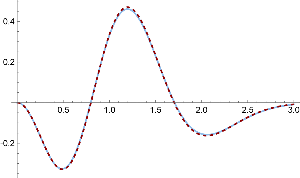
 is as in (2.10), with the Fredholm determinant herein computed according to Bornemann’s method [Reference Bornemann6, Reference Bornemann7], shows the same high level of graphical accuracy for the approximate leading correction term as does the Wigner surmise for the limiting distribution; see Figure 1.
[color-on-line] Exact functional form of
$\mathcal P_{1,\beta =2}(s;\xi)|_{\xi = 1}$
 (solid blue line) plotted together with the approximation obtained by substituting the Wigner surmise for
$\mathcal P_{0,\beta =2}(s;\xi)|_{\xi = 1}$
 in (2.8) (dashed red line).

Figure 1 Long description
The horizontal axis is labeled with values from 0 to 3. The vertical axis ranges from approximately negative 0.3 to 0.5. Two curves are plotted: a solid blue line and a dashed red line. Both curves start at the origin, dip to a minimum near x equals 0.4, rise to a peak at about x equals 1.2 with a maximum near 0.5, descend to a trough at x equals 2 with a minimum near negative 0.25, and then rise again toward x equals 3. The dashed red line closely follows the solid blue line throughout, with no visible divergence between the two curves at any point along the x-axis.
2. For a fixed N, the quantity
$(2 \pi /N)^2 \mathcal P_N^{\mathrm {CUE}}(2 \pi s / N;\xi )$
 can be computed empirically from numerically generated eigenvalues of CUE matrices for all
$0 < \xi \le 1$
 . Thus for
$\xi = 1$
 this is just the spacing distribution for consecutive eigenvalues, while for
$0< \xi < 1$
 it is the spacing distribution after deleting each eigenvalue with probability
$(1-\xi )$
 [Reference Bohigas and Pato5]. Subtracting this from
$\mathcal P_{0,\beta =2}^{\mathrm {bulk}}(s;\xi )$
 and scaling by
$N^2$
 will then give the graph of
$\mathcal P_{1,\beta =2}(s;\xi )|$
 up to corrections of order
$1/N^2$
 . In accordance with an hypothesis first put forward by Keating and Snaith [Reference Keating and Snaith53] and further developed in [Reference Bogomolny, Bohigas, Leboeuf and Monastra4, Reference Forrester and Mays35, Reference Bornemann, Forrester and Mays14], this same effect holds true for the empirical determination of
$\mathcal P_N^{(\cdot )}(x;\xi )$
 for the Riemann zeros at large height. Indeed one can observe (up to scaling and statistical fluctuations) the graphical form of Figure 1 in the analysis of the latter carried out in [Reference Bogomolny, Bohigas, Leboeuf and Monastra4, Reference Forrester and Mays35] – see in particular [Reference Forrester and Mays35, Fig. 10].
3. The structure of (2.8) shows immediately that
$\int _0^\infty s^j \mathcal P_{1,\beta =2}^{\mathrm {bulk}}(s;\xi ) \, ds = 0$
 for
$j=0,1$
 . To anticipate this, note from the finite N definition of
$\mathcal P_N^{(\cdot )}(x;\xi )$
 (2.1), that the requirements that for the normalisation and the first moment
$\int _0^\infty x^j p_N^{(\cdot )}(k;x) \, dx = 1 \, (j=0)$
 and
$k \, (j=1)$
 (the latter with bulk scaling, density unity, imposed) tell us
$\int _0^\infty s^j \mathcal P_{1,\beta =2}^{\mathrm {bulk}}(s;\xi ) \, ds$
 for
$j=0,1$
 is independent of N.
4. In the extension of the expansion (1.21) as an asymptotic series in powers of
$N^{-2/3}$
 , the explicit form of the functional form at order
$N^{-4/3}$
 is given as
$\sum _{l=1}^4 p_l(t) {d^l \over d t^l} E_{\beta = 2}^{\mathrm {soft}}((t,\infty );\xi )$
 for certain (low order) polynomials
$\{ p_l(t) \}$
 , with analogous functional forms conjectured at higher order (made explicit at order
$N^{-2}$
 ) [Reference Bornemann11, Reference Bornemann13]. However, in relation to
${\mathcal P}^{\mathrm {bulk}}_{2,\beta =2}(s;\xi )$
 in (2.3), we have yet to find evidence for a generalisation of (2.8) using as data the power series in (2.4) and (2.6). For the two-point correlation function which is the
$\xi = 0$
 case of
$\mathcal P_{0,\beta =2}(s;\xi )$
 , from the explicit functional form exhibited by extending the expansion (1.11) to O
$(N^{-4})$
 , one can check that

cf. (2.7). However, as a candidate for linking the O
$(N^{-4})$
 term for the spacing generating function to its limiting form, this is incompatible with the
$\xi $
 -dependent terms in (2.4) and (2.6). In Appendix B we provide further data on the relation between the powers series (2.4), and (2.5) and (2.6), for the leading small-s term at each power of
$\xi $
 .
3 Bulk scaling expansion of the correlations for
$\beta = 1$
and
$\beta = 4$


3.1 Pfaffian point process viewpoint
The eigenvalue PDF (1.7) with
$\beta =1$
 and
$4$
 corresponds to circular orthogonal and symplectic ensembles, respectively, denoted COE and CSE, which are known to form Pfaffian point processes (see, e.g., [Reference Forrester29, Ch. 6]). Specifically, the k-point correlation functions have the Pfaffian form

where the kernels are given by
$2\times 2$
 matrices

Here the entries are given by functions

where
$\epsilon _N(\theta )$
 depends on the parity of N [Reference Mehta59, §11.3]

In the bulk scaling, unlike
$\frac {1}{N}S_N({2 \pi X\over N})$
 , the scaled functions
$D_N,I_N$
 and
$J_N$
 are odd functions in N. Nevertheless, the n-point correlation functions are still even in N which can be seen through the fact that the functions
$I_N$
 (
$J_N$
 )/
$D_N$
 appear exclusively in the odd/even rows of the Pfaffian. Of particular interest are the functional forms of the leading correction in comparison to the limit itself (these functional forms being classical [Reference Mehta59]) in the case of the two-point function.
Proposition 3.1. For
$\beta =1,4$
 , and for certain functional forms
$\{ \rho _{(n),l,\beta }^{\mathrm {bulk}} \}_{l=0,1,\dots ,}$
 , we have

Specifically, in the case
$n=2$
 of the two-point correlation

where
$ \mathrm {Si}(x):=\int _0^x \frac {\sin t}{t}dt$
 .
A differential relation relating the functional form of the leading correction to the limiting functional form analogous to (2.7) can be observed.
Corollary 3.1. For
$\beta = 1,4$
 we have

with
$c_1 = - {1 \over 6}, c_4 = - {1 \over 24}$
 .
Proof. This is verified using computer algebra from the explicit functional forms.
3.2 Spacing distributions
We have from [Reference Bornemann, Forrester and Mays14, Cor. 5.12] the
$\beta = 1$
 spacing distribution expansions analogous to (2.4) and (2.5)


To the order shown, these spacing distribution generating functions, and the gap probability generating functions
$ \mathcal E_{0,\beta =1}^{\mathrm {bulk}}(s;\xi ), \mathcal E_{1,\beta =1}^{\mathrm {bulk}}(s;\xi )$
 too, are related by the analogues of (2.8) and (2.9)

the first of which with
$\xi = 0$
 reduces to the case
$\beta =1$
 of (3.3). In fact these identities (since they are equivalent to each other, it suffices to consider only the second) can be established to be true in general.
For this purpose, we will use that fact that analogous to (2.10) and (2.12), the gap probability generating functions in (3.6) admit forms relating to certain integral operators. As already commented, the circular ensemble for
$\beta = 1$
 is the circular orthogonal ensemble, which gives rise to a Pfaffian point process. These imply matrix Fredholm determinant forms (specifically the kernel of the corresponding integral operator is a
$2 \times 2$
 matrix) for the generating functions. We require instead a relation to certain scalar integral operators. This comes about due to the generating function identity ([Reference Forrester29, Eq. (8.150)
$N$
 even case], [14, Prop. 5.1 & Eq. (5.10)])

where
$\nu = (-)^N$
 and
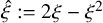
$\hat {\xi } := 2 \xi - \xi ^2$
 . In (3.7) the notation
$O^+(n)$
 and
$O^-(n)$
 refers to the eigenvalues in
$(0,\pi )$
 of these classical matrix groups, while COE
${}_N$
 refers to the
$N \times N$
 circular orthogonal ensemble. The eigenvalues of the classical groups orthogonal ensembles form determinantal point processes with respective kernels (see, e.g., [Reference Forrester29, §5.5.2])

Expanding the bulk scaling of the RHS of (3.7) for large N according to (1.10) gives


Here
$\mathcal K_s^\pm $
 and
$\mathcal L_s^\pm $
 are the integral operators on
$(0,s)$
 with kernels

where
$K_\infty , L_\infty $
 are given by (1.6) and (2.11) respectively. Let us denote
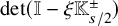
$\det (\mathbb I - {\xi } \mathbb K_{s/2}^\pm )$
 by
$\mathcal E_{0}^\pm (s;\xi )$
 and
$\det (\mathbb I - {\xi } \mathbb K_{s/2}^\pm ) \mathrm {Tr}(( \mathbb I - \xi \mathbb K_{s/2}^\pm )^{-1} \xi \mathbb L_{s/2}^\pm )$
 by
$\mathcal E_{1}^\pm (s;\xi )$
 . We can establish the following differential identity between these quantities, which is sufficient for the validity of (3.6).
Proposition 3.2. We have

Proof. As with Proposition 2.1, our strategy is to make use of Painlevé transcendent characterisations of the quantities in (3.11). Specifically, in [Reference Bornemann, Forrester and Mays14, Prop. 5.10]
$ \mathcal E_{0,\beta =1}^{\pm }(s;\xi )$
 was expressed as particular
$\sigma $
 PIII
$'\, \tau $
 -functions, involving certain transcendents
$f_0^\mp $
 . The structure of
$ \mathcal E_{1,\beta =1}^{\pm }(s;\xi )$
 was shown to be analogous to (2.16), and thus involving transcendents
$f_1^\mp $
 specified by the solution of a second order linear differential equation analogous to (2.17) subject to certain boundary conditions. The identity (3.11) is then seen to be equivalent to an identity analogous to (2.19) expressing
$f_1^\mp $
 in terms of
$f_0^\mp $
 . This in turn can be established following the procedure used to establish (2.19).
The identity (3.11) also has relevance to the
$\beta = 4$
 analogue of (2.8), (2.9) and (3.6).
Proposition 3.3. We have

Proof. First, as already commented in relation to (2.8) and (2.9), the two identities are equivalent, so it suffices to consider only the second of these. In the case of the CSE (i.e., the circular
$\beta $
 ensemble with
$\beta = 4$
 ), we have that [Reference Forrester29, Eq. (5.15)] (for context see the recent review [Reference Forrester32, §3.3])

Consequently

where use has been made of the notation introduced above Proposition 3.2; cf. the rewrite of (3.9) and (3.10) using this notation – note in particular a further factor of
$1/4$
 appearing on the RHS of
$\mathcal E_{1,\beta = 4}((0,s);\xi )$
 relative to
$\mathcal E_{1,\beta = 1}((0,s);\xi )$
 , which is traced back to the occurrence of the dimensions of the orthogonal groups on the RHS of (3.13) being
$2N+1$
 rather than
$N+1$
 as in (3.7).
3.3 The structure function expanded for large N
The structure function (also known as the spectral form factor)
$S_{N,\beta }(k)$
 is defined in terms of the Fourier coefficients of the truncated two-point correlation
$\rho _{(2),N}^T(0,\theta ;\beta ) = \rho _{(2),N}(0,\theta ;\beta ) - ( N / 2 \pi )^2$
 according to

where the additive constant term ensures that
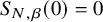
$S_{N,\beta }(0)=0$
 . In the case
$\beta = 2$
 it follows from (1.3) and (1.4) that

Consequently we obtain the now classical (see, e.g., [Reference Haake46]) exact evaluation

Consider next the bulk scaling of the structure function

Recalling (1.5) we see that (3.18) is, up to the additive constant, the Fourier transform in the Fourier variable
$2 \pi \tau $
 of the truncated two-point correlation in bulk scaling variables. To obtain the large N form for
$\beta =2$
 , one may trial making use of (1.11). However doing so leads to an ill-defined integral at order
$1/N^2$
 . Rather, from the exact result (3.17) we see that

and thus, as the RHS is independent of N, all terms in the corresponding large N expansion in fact vanish except the leading term.
The explicit leading corrections for
$\beta =1$
 and 4 of Proposition 3.4 show that it is similarly not possible to obtain meaningful large N expansions of the bulk scaled structure function by substituting in (3.18) the large N expansion of the bulk scaled two-point correlation. Instead one should use knowledge of the exact form of the structure function for these
$\beta $
 values at finite N [Reference Haake, Kus, Sommers, Schomerus and Zyczkowski47, Reference Witte and Forrester76],

and

where
$\psi (z)$
 denotes the digamma function.
Proposition 3.4. We have that for large N

and

Furthermore, in both cases the terms not shown are a series in
$N^{-2}$
 , starting at order
$N^{-4}$
 .
Proof. In all cases except
$\beta = 4$
 with
$|\tau | \le 1$
 , the stated expansions follow from (3.20) and (3.21) together with the large z asymptotic expansion of the digamma function [72]

In the case
$\beta = 4$
 with
$|\tau | \le 1$
 , we must first rewrite
$ \psi (-N+|k|+1/2)$
 using the reflection formula for the digamma function,

before making use of (3.24).
To deduce that all the terms in the large N asymptotic expansion are in powers of
$N^{-2}$
 , we first eliminate the shift by
$1/2$
 in the arguments of the digamma functions in (3.20) and (3.21) by using the identity [73]

where
$\gamma $
 denotes Euler’s constant and
$H_n$
 denotes the harmonic numbers. Use of the large n asymptotic expansion [73]

then establishes the result.
According to Proposition 3.4, for
$\beta = 1$
 and 4 at least the bulk scaled structure function has the large N asymptotic expansion

where the higher order terms are a series in
$1/N^2$
 starting at order
$1/N^6$
 . From the explicit expansions (3.22) and (3.23) (further extended to order
$1/N^4$
 ), we observe the differential relations for
$\beta =1,4$
 (where it has been assumed that
$\tau> 0$
 , which then removes the absolute value signs in the expressions of Proposition 3.4)

with
$c_1 = -{1 \over 6}, c_4 = - {1 \over 24}$
 ,
$d_1 = {7 \over 360}, d_4 = {7 \over 5760}$
 .
For small
$\tau $
 and general
$\beta> 0$
 we have available from [Reference Witte and Forrester76, Corollary 4.1] the small
$|\tau |$
 expansion of the terms on the RHS of (3.28) up to and including
$\mathrm {O}(\tau ^{11})$
 for
$ \tilde {S}_{0,\infty ,\beta }(\tau )$
 (the final order term was obtained in the subsequent work [Reference Forrester30]), to order
$\tau ^8$
 for
$ \tilde {S}_{1,\infty ,\beta }(\tau )$
 , and to order
$\tau ^6$
 for
$ \tilde {S}_{2,\infty ,\beta }(\tau )$
 . For present purposes we will be content with presenting these expansions to smaller order than what is available. For this, we define the polynomials

Here
$\kappa := \beta /2$
 . In terms of these polynomials one has from [Reference Witte and Forrester76] the small
$\tau $
 expansions


These general
$\beta $
 expansions (3.30) and (3.31) are seen to be consistent with the first differential relation in (3.29) with
$c_\beta = - {1 \over 12 \kappa }$
 , while (3.30) and (3.32) are consistent with the second differential relation with
$d_\beta = (\kappa ^3 - 1)/(720 \kappa ^3 (\kappa - 1))$
 .
Remark 3.1. 1. The limiting functional forms of
$ \tilde {S}_{N,\beta }(\tau )$
 are classical results in random matrix theory (see [Reference Dyson23, Eq. (5.6) for
$\beta =1$
 ] and [Reference Mehta59, equivalent to Eq. (7.2.46) for
$\beta =4$
 ]).
2. By inspection the expansions (3.30)–(3.32) are unchanged (up to a minus sign) by the mappings
$\kappa \mapsto 1/\kappa $
 and
$\tau \mapsto - \tau /\kappa $
 . This is consistent with the known functional equation [Reference Witte and Forrester76, Prop. 4.7]. Also, previously the polynomials of
$\kappa $
 appearing in (3.30) have been observed to have all their zeros on the unit circle in the complex
$\kappa $
 plane, and which display an interlacing property [Reference Witte and Forrester75], [Reference Forrester and Shen39]. This is similarly true of the polynomials in (3.31) and (3.32).
4 Bulk scaling expansion of the correlations for even
$\beta $

4.1 Hypergeometric functions based on Jack polynomials
In the cases
$\beta = 1,2$
 and 4 the general k-point correlation function for the circular
$\beta $
 ensemble is fully determined by a certain scalar kernel function (1.9) for
$\beta = 2$
 , and by a matrix kernel function (3.1) for
$\beta = 1$
 and 4. Generally, from (1.7) and the
$\beta $
 version of (1.2), the cases of
$\beta $
 even have the special property that the k-point correlation function is a Laurent polynomial in
$\{e^{i \theta _j} \}_{j=1,\dots ,k}$
 . In the work [Reference Forrester26] this polynomial was identified in terms of a (then) recently introduced class of generalised hypergeometric functions based on Jack polynomials [Reference Kaneko52]. To define these hypergeometric functions we must then first introduce Jack polynomials [Reference Macdonald58, Ch. VI.6], [Reference Forrester29, Ch. 12], [Reference Kuramoto and Kato55, Ch. 7].
Jack polynomials
$P_\kappa ^{(\alpha )}(\mathbf x)$
 are symmetric polynomials of N variables
$\mathbf x = (x_1,\dots ,x_N)$
 . They are labelled by a partition
$\kappa := (\kappa _1,\dots ,\kappa _N)$
 with parts which are non-negative integers ordered as
${\kappa _1 \ge \kappa _2 \ge \cdots \ge \kappa _N}$
 , and dependent on a parameter
$\alpha> 0$
 . They have the triangular structure with respect to the monomial basis
$\{ m_\mu (\mathbf x) \}$


In (4.1) the notation
$\mu < \kappa $
 denotes the partial order on partitions, defined by the requirement that for each
$s=1,\dots ,\ell (\kappa )$
 (where
$\ell (\kappa )$
 denotes the number of nonzero parts of
$\kappa $
 ) we have
$\sum _{i=1}^s \mu _i \le \sum _{i=1}^s \kappa _i$
 . The Jack polynomial
$P_\kappa ^{(\alpha )}(\mathbf x)$
 can be specified as the unique polynomial eigenfunctions of the differential operator

with the structure (4.1).
The special case
$\alpha =2$
 of the Jack polynomials corresponds (up to normalisation) to the zonal polynomials of mathematical statistics; see, for example, [Reference Muirhead63, Ch. 7]. In this case, generalised hypergeometric functions of the type of relevance to the circular
$\beta $
 ensemble were introduced in a work of Herz [Reference Herz49], albeit entirely in the context of matrix integrals, and without reference to zonal polynomials. A series definition involving zonal polynomials came in the later work of Constantine [Reference Constantine19]. Generalising this, Yan [Reference Yan77] and Kaneko [Reference Kaneko52] introduced the family of hypergeometric functions based on Jack polynomials as

Here, with
$\mathbf x = \{x_i\}_{i=1}^m$
 , the sum is over all partitions
$\kappa _1 \ge \kappa _2 \ge \cdots \ge \kappa _m \ge 0$
 , and conventionally the sum is performed in order of increasing
$|\kappa |$
 . Also use has been made of the generalised Pochhammer symbol

see, for example, [Reference Forrester29, Eq. (12.46)]. For the precise definition of
$h_\kappa '$
 (which also depends on
$\alpha $
 ) we refer to, for example, [Reference Forrester33, Eq. (3.4)]. Recent works making essential use of this class of hypergeometric function in contexts relating to random matrix theory include [Reference Feng and Wei25, Reference Forrester31, Reference Novak65, Reference Winn74, Reference Liu, Wang, Yang and Zhao56].
4.2 Evenness of the correlation functions in N
Deduced in [Reference Forrester26], and conveniently summarised in [Reference Forrester29, Prop. 13.2.1], one has that the n-point correlation function for circular
$\beta $
 ensemble with even
$\beta $
 in bulk scaling variables

has the evaluation in terms of the generalised hypergeometric function

where

and
$M_{N-n}$
 is the Morris integral (see, e.g., [Reference Forrester29, Eq. (4.4)])

We note that the RHS of (4.5) gives meaning to
$\tilde {\rho }_n$
 for continuous N. In fact, as already demonstrated above for
$\beta = 1,2$
 and 4 as properties of the underlying correlation kernels, this can be shown to be even in N.
Proposition 4.1. Fix n independent of N and such that
$2n < N$
 . We have that (4.5) is an even function of N.
Proof. The first observation is that by using the transformation formula (see, e.g., [Reference Forrester29, Prop. 13.1.6])

it follows that the second line of (4.5) is even in N. It is immediate that the product
$\prod _{1\leq j<k\leq n}|e^{2\pi ir_k/N}-e^{2\pi ir_j/N}|^\beta $
 is also invariant under negation of N. The remaining factor, after substitution of the Morris integral formula, is

Assume that
$N>2n$
 and denote
$\beta /2=\kappa $
 as used in the paragraph below (3.29), then the cancellation in the product of the gamma functions yields

in which the N-dependent part is

This can then be further simplified to give

which is thus also even in N, and so all factors in (4.5) are even in N.
It follows from Proposition 4.1 that if, for
$\beta $
 even, the existence of an asymptotic expansion in inverse powers of N can be established, then in fact the expansion is in inverse powers of
$N^{-2}$
 . Work relevant to establishing that the generalised hypergeometric function in (4.5) permits an expansion in
$1/N$
 up to order
$1/N^2$
 at least has been given in the recent work [Reference Winn74] (strictly speaking the dependence on N in the case of the particular
${\vphantom {F}}_2^{\mathstrut } F_1^{(\alpha )}$
 appearing in [Reference Winn74] is different from its appearance in (4.5) so this is not immediate). However, restricting attention to the two-point correlation, one has available a particular
$\beta $
 -dimensional integral form of the required generalised hypergeometric function from which the existence of a
$1/N$
 expansion is easy to establish. This integral form reads [Reference Forrester28], [Reference Forrester29, Prop. 13.2.2, after deleting a spurious prefactor
$\left(\beta N/2\right)!$
 ],

Here
$S_n(a,b,c)$
 is the Selberg integral (see, e.g., [Reference Forrester29, §4.1]), which for the stated parameters is such that the multiple integral is normalised to unity for
$r_1-r_2=0$
 .
Proposition 4.2. The RHS of (4.12) admits an asymptotic expansion in
$1/N$
 . Combining this with Proposition 4.1 gives the
$1/N^2$
 expansion

for some
$\{ \rho _{(2),l,\beta }^{\mathrm {bulk}}(x,0) \}_{l=1,2,\dots }$
 , and where

Proof. With
$A_N(x) := 1 + \sum _{l=1}^\infty {(2\pi ix)^l \over (l+1)! N^l}$
 , we write

Since for fixed x this expression admits a
$1/N$
 expansion, uniform in the integration variables on their domain of support, it follows immediately that the multi-dimensional integral similarly admits a
$1/N$
 expansion. In addition, the working of the proof of Proposition 4.1 shows that all the prefactors to the multi-dimensional integral admit
$1/N$
 expansions, which then as said is lifted to a
$1/N^2$
 expansion according to the result of Proposition 4.1. The explicit form of the limit (4.14), already known from [Reference Forrester28], can be read off by keeping track of the leading order terms throughout.
4.3 Functional form of the
$1/N^2$
correction for the two-point function

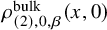
Starting with (4.12), it is possible to deduce the generalisation of the formulas (2.7) and (3.3) linking the first correction
$\rho _{(2),1,\beta }^{\mathrm {bulk}}(x,0)$
 in (4.13) to the limit
$\rho _{(2),0,\beta }^{\mathrm {bulk}}(x,0)$
 for all even
$\beta $
 .
Proposition 4.3. With reference to the asymptotic expansion (4.13), for all even
$\beta $
 we have

Proof. In order to obtain the functional form of the
$1/N^2$
 correction, we start from the calculation of the
$1/N$
 expansion of the integral

Introduce the notation

Let
$\theta =2\pi x$
 , then by substituting the expansion up to terms O
$(N^{-3})$


we see that (4.17) can be expanded up to terms O
$(N^{-3})$
 as

The integrals in the above expansion can be evaluated by performing integration by parts on each variable
$u_j$
 and then taking the sum. This general strategy was introduced into the wider theory of Selberg integrals by Aomoto [Reference Aomoto2]; see [Reference Forrester29, §4.6] for more on this. With

taking the partial derivative on each side of
$u_k^m(1-u_k)^nf(u)$
 gives

Starting from the simplest case with
$m=n=1$
 , using integration by parts, this shows

where we have used the formula

Similar calculations show

and

Substituting the above equations in (4.18), we see that (4.17) can be written up to terms
$\mathrm {O}(N^{-3})$


where we have used the simple relations

Now we look at the prefactors in (4.12). After simplification, we have

For large N

Multiplying the implied
$1/N$
 expansion of the prefactors with the
$1/N$
 expansion (4.19) shows that the first correction in (4.13) (i.e., the coefficient of
$1/N^2$
 ) is given by

where

By substituting the latter equation into (4.20), the stated relation (4.16) follows.
Remark 4.1. 1. In Appendix A, it is shown that the above calculations can be generalised to a recurrence relation among

which can be used to show that the higher order corrections in (4.13) are related to a finite sum over derivatives of the limit, where the coefficients in the sum are polynomials.
2. As well as conjecturing that (4.16), proved now for even
$\beta $
 and
$\beta =1$
 , holds true for general
$\beta> 0$
 , we can conjecture too that so does the
$\beta $
 generalisation of (2.8), (3.6) and (3.12),

with (4.16) corresponding to the case
$\xi =0$
 . Further evidence for this is presented in Appendix B, where it is shown that (4.22) is valid for the leading s powers at each order
$\xi ^k$
 in the bulk scaling expansion of (2.3).
Appendix A
Here a recurrence relation for the quantities (4.21) will be deduced, which has consequences for the functional form of the higher order corrections in (4.13). For this purpose, given an integer m, introduce the notations

Denote by
$\tau =(\tau _1,\dots ,\tau _n)$
 a partition of m with length
$|\tau |=n$
 . Associate to
$\tau $
 a partition
$s_\tau $
 of
$|\tau |$
 , that is,
$s_\tau =(s_1,\dots ,s_k)$
 satisfying
$\sum _{i=1}^{k}s_i=n $
 , with each component indicating the number of identical elements in
$\tau $
 . As a set of integers, we adopt the notation
$\tau !=\tau _1!\tau _2!\dots \tau _n!$
 . We have the following recursive identity.
Proposition A.1. For any set of integers
$a^{[m]}$
 with
$a_1\geq 2$
 , the integrals
$\mathcal {I}^{(m)}(a_1,a_2,\dots ,a_m)$
 satisfy the recurrence relation

where

The initial conditions
$\mathcal {I}^{(m)}(0,\dots ,0,1,\dots ,1)$
 can be determined in terms of
$\partial _\theta ^m \mathcal {I}[1], m\in \mathbb {Z}_{\geq 0}$
 by

and

Proof. Integration by parts shows

The summation in the last integral can be separated into two sums

By interchanging the summation indices, the first sum can be written as

Similarly, the second sum equals

Therefore, after substituting these into (A.2), equation (A.1) is proved. The equations for the initial conditions can be seen from the formulas

Remark A.1. From the expansion of
$\prod _{j=1}^\beta \left (1-\left (1-e^{ i\theta / N}\right ) u_j\right )^{N-2}$
 , one knows that the multiple integral in (4.12) can be written as a linear combination of
$\mathcal {I}^{(m)}(a_1,a_2,\dots ,a_m)$
 , which upon use of Proposition A.1 can be expressed in terms of
$\theta $
 -derivatives of the leading term
$\mathcal {I}[1]$
 . Therefore, all the higher-order correction terms of the two-point correlation can be expressed as a finite linear combination of the derivatives of the leading term with coefficients being polynomials in
$\theta $
 . However, to make this explicit beyond the
$N^{-2}$
 term, in particular for the
$N^{-4}$
 term, would be an arduous task due to the many terms involved and multiple cancellations. In the case
$\beta =2$
 , it was noted in (2.20) that a simple differential relation linking
$\rho _{(2),2,\beta =2}^{\mathrm {bulk}}(s,0)$
 and
$\rho _{(2),0,\beta =2}^{\mathrm {bulk}}(s,0)$
 can be read off from the respective exact functional forms.
Appendix B
It turns out that the leading small-x (small-s after introducing scaled variables) form of the coefficient of
$\xi ^k$
 in (2.1) can be determined, along with the N-dependent factor multiplying this term. According to (2.2) and (1.15), for
$\beta = 2$
 , and with bulk scaling as on the LHS of (2.3) (scaled variable s) we read off that for
$k=0$
 and
$k=1$
 respectively, the leading small-s coefficients of
$\xi ^k$
 are

The significance of knowledge of this is that it provides necessary conditions for the differential identity (2.8), as each such coefficient of
$\xi ^k$
 must independently have its N-independent part related to the
$N^{-2}$
 -dependent part according to (2.8), and similarly should there be such relations for parts at order
$N^{-4}$
 etc.
Proposition B.1. Consider (2.1) for the circular
$\beta $
 ensemble with bulk scaled variables as on the LHS of (2.3). The leading small-s coefficient of
$\xi ^k$
 is, for
$n:=k+2 < N/2$
 and
$\kappa := \beta /2$
 a positive integer, equal to

Proof. Analogous to the structure of (4.5) in the limit of small
$\{r_j\}$
 , when to leading order all the
$r_j$
 dependent terms on the second line can be set equal to unity, in this regime we have for the general
$\beta> 0$
 bulk scaled n-point correlation

The relevance of this to (2.1) with bulk scaling as on the LHS of (2.3) is seen by changing variables in the multiple integrals therein
$x_j \mapsto 2 \pi s x_j/N$
 . The integrand can then be substituted by (B.3), showing that to leading order for s-small, the coefficient of
$\xi ^k$
 is given by

Here
$S_k$
 refers to the Selberg integral. According to the working of the proof of Proposition 3.4, the second line simplifies to the second line of (B.4), and thus the result.
The N-dependent factors in (B.4), namely
$N^{-\kappa n (n-1)} $
 times the double product on the second line, with
$n=k+2$
 , have the large N form

where
$v_s(\kappa ) := \kappa ^{-2}\sum _{j=1}^{n-1} \sum _{l=1}^{j \kappa } l^s$
 . In particular

Since
${1 \over 6 \beta } {d^2 \over d s^2} s^{n + \kappa n (n - 1)} = v_2(\kappa ) s^{(n-2) + \kappa n ( n - 1)}$
 , where the term being differentiated on the LHS is the s-dependent factor in (B.2) times
$s^2$
 , we see that there is consistency with the conjecture (4.22). The coefficient of
$N^{-4}$
 in (B.5) is an order eight polynomial in n, telling us that if there were to be an analogue of (4.22) at this order, the highest power derivative must be four.
Acknowledgments
Correspondence with F. Bornemann relating to this work has been appreciated.
Competing interests
The authors have no competing interest to declare.
Funding statement
This work was supported by the Australian Research Council Discovery Project grants DP210102887 and DP250102552.




 Open access

