1. Introduction
Blowout and thermoacoustic instability are two challenges that we face while operating combustors in lean premixed conditions (Lieuwen & Yang Reference Lieuwen and Yang2005). Blowout occurs when the flame ceases to exist inside the combustor. Blowout can happen either through flame blow-off or flame extinction. On the other hand, thermoacoustic instability refers to the large-amplitude acoustic oscillations that are established inside a combustor when the unsteady heat release rate from the combustor has a positive feedback with the acoustic perturbations. Near fuel-lean limits, combustors are susceptible to blowout and thermoacoustic instability due to the increased sensitivity of the flame to the flow perturbations.
There have been extensive studies regarding the dynamics of blowout and thermoacoustic instability near lean limits. Initial studies focused on finding the stability margins for flame blowout and thermoacoustic instability for various combustor configurations. In this context, lean blowout is described as loss of static stability of the flame since the static stability of the reaction is lost at blowout (Lieuwen Reference Lieuwen2007). In contrast, thermoacoustic instability is considered as a loss of dynamic stability of the combustor (Lieuwen & Yang Reference Lieuwen and Yang2005; Lieuwen Reference Lieuwen2007), as the instability is characterized by large-amplitude oscillations that are characteristic of a dynamically unstable system.
Nevertheless, recent studies focusing on nonlinear dynamics of combustors show that the transition to both thermoacoustic oscillations and blowout exhibits dynamically rich behaviour. Kabiraj & Sujith (Reference Kabiraj and Sujith2012) discovered intermittent dynamics in a thermoacoustic system with laminar premixed combustion. They identified that prior to blowout the thermoacoustic system exhibited intermittency, where the system switched from low-amplitude periodic fluctuations to high-amplitude chaotic fluctuations. From the analysis of pressure fluctuations in a combustor with turbulent flame, Gotoda et al. (Reference Gotoda, Amano, Miyano, Ikawa, Maki and Tachibana2012) established that the phase space corresponding to combustion oscillations prior to blowout exhibited multifractal characteristics. They also evaluated the degree of multifractality in terms of the equivalence ratio of combustion. They further emphasized that a multifractal analysis is indeed necessary to understand the nonlinear dynamics associated with these oscillations and that simple measures such as the divergence of phase space trajectories could not capture the rich dynamics at the blowout limit. In another recent study, Gotoda et al. (Reference Gotoda, Shinoda, Kobayashi, Okuno and Tachibana2014) described that the translation error, which quantifies the degree of parallelism of trajectories in the phase space, can be used as a control variable to detect lean blowout (LBO). Further, Domen et al. (Reference Domen, Gotoda, Kuriyama, Okuno and Tachibana2015) suggested that permutation entropy, quantifying the rank order pattern of components in phase space vectors constructed from the short time-series data of pressure fluctuations, can also be used as a control variable to prevent LBO. All these studies point to the nonlinear nature and complexity of combustion dynamics prior to blowout.
In a study of dynamics of the onset of thermoacoustic instability, Nair et al. (Reference Nair, Thampi, Karuppusamy, Gopalan and Sujith2013) reported that combustion noise from a turbulent flame confined in a combustor is chaotic and described the transition from combustion noise to thermoacoustic oscillations as a transition from chaos to order. They (Nair & Sujith Reference Nair and Sujith2013; Nair, Thampi & Sujith Reference Nair, Thampi and Sujith2014) also observed that the transition region is characterized by intermittent oscillations where the system switches from low-amplitude aperiodic oscillations to high-amplitude periodic oscillations. Further, Nair & Sujith (Reference Nair and Sujith2014) showed that the ‘combustion noise’ generated by a flame in a confined environment has multifractal characteristics and is not merely stochastic fluctuations. They showed that the ‘noise’, which in general is either filtered out or treated as stochastic background in traditional analysis and modelling of combustion dynamics (Noiray & Schuermans Reference Noiray and Schuermans2013), does contain important information about the dynamical state of the system. Further, they also suggested that the ‘noise’ might be a direct consequence of inherent complexity of turbulent combustion dynamics, and hence the separation of the measurements into a signal and noise may lead to loss of valuable information.
Considering the complex nature of dynamics at the transition to blowout, it seems that a mere description of blowout as loss of static stability of the flame is inadequate. Further, it is evident from prior research (Nair & Sujith Reference Nair and Sujith2014) that even the so-called stable dynamics in the context of stability analysis (i.e. combustion noise) is highly complex. In the context of the onset of thermoacoustic oscillations, Nair & Sujith (Reference Nair and Sujith2014) addressed this problem by adopting a multifractal description of combustion noise and describing the onset of thermoacoustic instability as a loss of multifractality. This description gives a clearer definition to the stability margin for the onset of thermoacoustic instability in a turbulent combustor while being able to accommodate the complex dynamics seen prior to the onset of thermoacoustic instability. Further, they were able to provide a novel precursor, the Hurst exponent (a measure indicative of the fractal nature of a time series), to detect the onset of an impending thermoacoustic instability. Inspired by this work, in this paper we establish a multifractal description of lean blowout. Towards this purpose and to identify how the new description could help us better describe the phenomena of blowout, we will first look at a brief overview of the current description of blowout.
Longwell, Frost & Weiss (Reference Longwell, Frost and Weiss1953) and Spalding (Reference Spalding1955) proposed that LBO is influenced by the ratio between the resident time of the reactants in the combustor and the reaction time scale represented by Damkhöler number, Da. Here, the chemical time scale associated with combustion is calculated from laminar flame speeds and thermal diffusivity. Another approach is to look at blowout as a collective flamelet extinction event (Plee & Mellor Reference Plee and Mellor1979; Radhakrishnan, Heywood & Tabaczynski Reference Radhakrishnan, Heywood and Tabaczynski1981). In this context, the ratio of the flow speed to the flame speed is used to characterize blowout. Blowout happens when this ratio exceeds one at critical locations in the combustor (Chaudhuri et al. Reference Chaudhuri, Kostka, Renfro and Cetegen2010).
However, in practical applications, the flame exhibits highly unsteady behaviour prior to blowout. A detailed study of this behaviour was performed by De Zilwa, Uhm & Whitelaw (Reference De Zilwa, Uhm and Whitelaw2000) using high-speed flame images and pressure fluctuation signals from a turbulent combustor. Chaudhuri et al. (Reference Chaudhuri, Kostka, Renfro and Cetegen2010) used time-resolved chemiluminescence imaging along with simultaneous particle image velocimetry (PIV) and OH planar laser-induced fluorescence (PLIF) to investigate the interaction between flame fronts and shear layer vortices prior to blowout. They reported that this interaction prior to blowout causes the local stretch rates in the flow to exceed the extinction stretch rates, resulting in local extinction of the flame. Further, Nair & Lieuwen (Reference Nair and Lieuwen2007) described the physical mechanism of flame blowout using the concept of growth of flame holes. The flame dynamics in specific combustor configurations and a more general review of the work on blowout are given by Shanbhogue, Husain & Lieuwen (Reference Shanbhogue, Husain and Lieuwen2009).
The dynamics of a flame near blowout was studied by Muruganandam (Reference Muruganandam2006) and Nair (Reference Nair2006) using signatures from acoustic perturbations and chemiluminescence measurements respectively. They observed burst-like behaviour prior to blowout in both signals. The burst count corresponding to these signals was then used as an indicator to detect an impending blowout. Further, Mukhopadhyay et al. (Reference Mukhopadhyay, Chaudhari, Paul, Sen and Ray2013) described the dynamics of blowout from its acoustic and chemiluminescence signature using symbolic time-series analysis and suggested a precursor (an indicative measure) to detect the proximity of a combustor to blowout. A more generalized form of this technique was introduced by Sarkar et al. (Reference Sarkar, Mukherjee, Sarkar and Ray2012). All the above studies indicate that blowout is indeed a dynamic problem, and simple descriptions based on loss of static stability and Damköhler correlations may not be adequate to describe this phenomenon.
Furthering this understanding of combustion dynamics prior to blowout, in this paper we address the following outstanding questions: Can we have a multifractal description of blowout and thus give a unified framework to describe blowout and thermoacoustic instability? If so, will such a description provide us a viable method of predicting an impending blowout? What can we understand from a multifractal description about the underlying physical mechanism of blowout? The rest of the paper is organized as follows. In § 2, we give a brief description of multifractality. The experimental set-up is described in § 3. The results and discussions of the experimental results are given in § 4. In § 5, we discuss the important conclusions from this study.
2. Multifractality
Fractals are geometric objects that exhibit self-similarity at different scales. As we zoom into a fractal, we can see similar structures emerging again and again at different levels of zoom. Due to this property of fractals, measures such as area and length of a fractal are dependent upon the scale of measurement. For example, if we were to measure the length of a curve that is a fractal using a ruler, the measured length of the curve follows an inverse power law with the length of the ruler used for measurement. Alternatively, a log–log plot of the measured length of the curve as a function of the length of the ruler is a straight line with a negative slope. The power-law exponent (the slope of the straight line in the log–log plot) is termed the fractal dimension
 $D$
. Euclidean objects have an integer fractal dimension equal to the physical dimension of the object. In contrast, fractals have a non-integer fractal dimension.
A similar concept can be used to characterize a fractal time series, where self-similarity is observed on various time scales. For a fractal time series
 $v(t)$
,
 $v(ct)=(c^{H})^{\ast }v(t)$
is also a signal with the same statistics (West et al.
Reference West, Latka, Glaubic-Latka and Latkam2003). Here,
 $H$
represents the Hurst exponent, a measure of the fractal dimension (
 $D$
) of the time series (Hurst Reference Hurst1951). The Hurst exponent
 $H$
can be related to the fractal dimension
 $D$
of the time series as
 $D=2-H$
. The algorithms that estimate the Hurst exponent from time-series data utilize this scaling relationship to derive the estimates. In practical situations, the scales present in a system have both upper and lower bounds that are dependent upon the characteristics of the system. Further, the signals might also exhibit complex scaling behaviour where the scaling factor is a function of the amplitude of fluctuations. Such time series are called multifractal time series and cannot be described using a single Hurst exponent (Mandelbrot Reference Mandelbrot1999). Hence, we need to define generalized Hurst exponents in order to describe their scaling behaviour.
A practical method that can be used to estimate the generalized Hurst exponents, called multifractal detrended fluctuation analysis (MFDFA), was introduced by Kantelhardt et al. (Reference Kantelhardt, Zschiegner, Koscielny-Bunde, Havlin, Bunde and Stanley2002). These generalized exponents indicate the scaling behaviour for the central moments of the time series appropriately scaled for various orders (both negative and positive). For example, the scaling of the standard deviation with time interval gives the Hurst exponent
 $H_{2}$
. For a monofractal signal, the generalized Hurst exponents (
 $H_{q}$
) have the same value for different
 $q$
, whereas for a multifractal signal, they have different values for different
 $q$
. In DFA, we represent this variation in the generalized Hurst exponents through a Legendre transformation. Under the transformation, the variation in generalized Hurst exponent at different orders is represented as a spectrum of singularities
 $f({\it\alpha})$
where
 ${\it\alpha}$
is the conjugate variable corresponding to
 $q$
. The width of the singularity spectrum gives the degree of multifractality in the signal.
In this work, we use MFDFA to study the multifractal characteristics of the pressure time series. However, the multifractal characteristics of the reconstructed phase space can also be analysed as shown by Gotoda and coworkers (Reference Gotoda, Amano, Miyano, Ikawa, Maki and Tachibana2012). They were able to identify the capacity dimension of the phase space by analysing the multifractal spectrum corresponding to the phase space attractor. However, from an online detection and control point of view, MFDFA is superior since the length of the time series and the computational time required for the analysis are much less for MFDFA. This is due to the fact that we avoid phase space reconstruction while performing MFDFA. One drawback of using MFDFA is that we will not be able to identify the attractor characteristics (such as capacity dimension of the attractor) using such an analysis. However, this does not hinder our purpose of predicting an impending blowout. The main analysis presented in this paper is based on MFDFA. Nevertheless, for completeness of the study, in the Appendix, we compare the multifractal characteristics of phase space attractors representing combustion noise and a state prior to blowout.
3. Experimental set-up
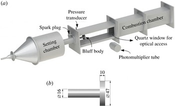
The combustor used for the present work is the test rig that was used by Nair & Sujith (Reference Nair and Sujith2014). It is a backward-facing step combustor with a bluff body used as the flame-stabilizing device. The combustion chamber has a cross-section of
 $90\times 90~\text{mm}^{2}$
. A spark plug mounted at the dump plane is used for ignition. The fuel used here is LPG (40 % butane and 60 % propane). The fuel is injected 120 mm upstream of the bluff body. Air is partially premixed with the fuel before the mixture enters the combustion chamber. The bluff body (figure 1
b) is a circular disc of thickness 10 mm and diameter 47 mm. Within the combustor, the bluff body is positioned 50 mm from the dump plane. The mass flow rates of fuel and air are measured using mass flow controllers (Alicat Scientific, MCR Series) with an uncertainty of
 $\pm$
(0.8 % of reading
 $+$
0.2 % of full scale). Unsteady pressure fluctuations were measured using a piezoelectric transducer (PCB103B02, uncertainty
 $\pm 0.15$
Pa). Chemiluminescence measurements were performed using a photomultiplier tube (PMT, Hamamatsu H10722-01). The PMT module was placed 50 mm from the quartz window normal to the plane of the window (figure 1
a). This position ensured that the photomultiplier captured the dynamics of the entire flame.
Schematic diagram of the lab-scale combustor used for this study. A pressure transducer, PCB103B02, is used to measure the pressure fluctuations in the system. The flame-stabilizing device is (b) a circular bluff body. The length of the combustion chamber can be changed by adding more sections in the combustor. For this study, the length was fixed at 1400 mm. The design of this combustor was adapted from Komarek & Polifke (Reference Komarek and Polifke2012).

The PMT module measures the filtered light intensity (narrow band, peak at 432 nm, 10 nm FWHM) corresponding to CH* chemiluminescence from the combustor. Thus at each instant of time, the PMT module is able to measure the total CH* chemiluminesence from the combustor, indicating the instantaneous rate of reaction or alternatively the heat release rate within the combustor. The collection cone angle for the PMT, for the particular configuration that is used in our experiments, is 4.65 sr. This ensures that we collect the light from the whole combustion zone. Any stray light is avoided by conducting the experiments in a dark room. The signals from the pressure transducer and the PMT module were acquired using an A–D card (NI-6143, 16 bit) at a sampling frequency of 10 kHz, for a duration of 3 s. In this study, we have represented the variation of various parameters with global equivalence ratio of the combustion mixture. Equivalence ratio is estimated as
 ${\it\varphi}=({\dot{m}}_{f}/{\dot{m}}_{a})_{\mathit{actual}}/({\dot{m}}_{f}/{\dot{m}}_{a})_{\mathit{stoichiometry}}$
. The uncertainty in the estimated equivalence ratio is
 $\pm 0.02$
.
It is to be noted that the choice of position of the pressure transducer does not affect the multifractal analysis as long as the pressure transducer is not at the pressure node of the standing wave and is able to capture the periodic fluctuations during thermoacoustic instability. However, we chose to locate the pressure transducer close to an acoustically closed boundary so that the periodic fluctuations corresponding to the standing wave oscillations have maximum amplitude at the measurement location.
4. Results and discussions
In this study, we aim to identify the multifractal characteristics of unsteady pressure signals and chemiluminescence signals from turbulent combustors prior to lean blowout. We conducted experiments at different fuel flow rates (1.04, 0.93, 0.81,
 $0.56~\text{g}~\text{s}^{-1}$
), each corresponding to different power levels of a combustor (18.2, 16.25, 14.3 and 9.75 kW respectively). In each experiment, the airflow rate is varied such that the equivalence ratio is decreased from 0.98 in discrete steps until the flame in the combustor blows out. The range of Reynolds number for the reported experiments is from
 $1.03\times 10^{4}$
to
 $3.7\times 10^{4}$
.
4.1. Dynamics of pressure and chemiluminescence oscillations
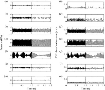
As the equivalence ratio is varied from near stoichiometry to blowout, we observe that pressure and CH* chemiluminescence signals exhibit various different temporal modulations. In figure 2 we illustrate these oscillations present in a bluff-body-stabilized combustor for a fuel flow rate of
 $1.04~\text{g}~\text{s}^{-1}$
. Here, we can identify that the transition from stoichiometric combustion to blowout follows the path: low-amplitude aperiodic oscillations
 $\rightarrow$
intermittency
 $\rightarrow$
thermoacoustic instability
 $\rightarrow$
intermittency
 $\rightarrow$
low-amplitude aperiodic oscillations
 $\rightarrow$
blowout.
At an equivalence ratio of 0.95, we observe that the pressure fluctuations have low amplitude and are aperiodic. Similarly the corresponding CH* chemiluminescence fluctuations are also aperiodic and have low amplitude. At an equivalence ratio of 0.80, we observe some periodic part in the time series alternating with aperiodic oscillations. This state is referred to as intermittency in dynamical systems theory. The existence of such intermittent dynamics in the transition region from combustion noise to thermoacoustic instability has been reported by Nair et al. (Reference Nair, Thampi and Sujith2014).
Variation of (a,c,e,g,i,k,m) pressure fluctuations and (b,d,f,h,j,l,n) CH* chemiluminescence fluctuations at different equivalence ratio conditions for a bluff-body-stabilized combustor operating in the turbulent regime. The fuel flow rate is
 $1.04~\text{g}~\text{s}^{-1}$
. At an equivalence ratio of 0.95 (
 $Re=1.13\times 10^{4}$
(a,b)) the pressure and CH* chemiluminescence fluctuations are aperiodic and have low amplitude. Further, the equivalence ratio is reduced by increasing the airflow rate, keeping the fuel flow rate constant. At an equivalence ratio of 0.80 (
 $Re=1.34\times 10^{4}$
(c,d)), we observed intermittency in both pressure and chemiluminescence signals. On further reduction of equivalence ratio to 0.68 (
 $Re=1.57\times 10^{4}$
(e,f)), we observe periodic behaviour for both pressure and chemiluminescence signals. At an equivalence ratio of 0.50 (
 $Re=2.14\times 10^{4}$
(g,h)), we still observe periodic oscillations. However, the amplitude of oscillations is higher than that at an equivalence ratio of 0.68. When the equivalence ratio is 0.47 (
 $Re=2.28\times 10^{4}$
(i,j)), we observe intermittency in both pressure and chemiluminescence signals with oscillations switching from high-amplitude periodic fluctuations to low-amplitude aperiodic fluctuations. When the equivalence ratio is further reduced, at an equivalence ratio of 0.44 (
 $Re=2.43\times 10^{4}$
(k,l)) the amplitude of periodic content in the oscillation reduces. When the equivalence ratio is 0.29 (
 $Re=3.69\times 10^{4}$
(m,n)) the pressure and chemiluminescence oscillations are aperiodic and have very low amplitude.

When the equivalence ratio is reduced to 0.68, we start observing periodic fluctuations in both pressure and chemiluminescence signals. On further reduction of the equivalence ratio, the amplitude of the periodic fluctuations (both chemiluminescence and pressure signals) increases. We can observe this by comparing the pressure and chemiluminescence signals corresponding to equivalence ratios of 0.68 and 0.50. The amplitude of periodic fluctuations is higher for the case with lower equivalence ratio. At an equivalence ratio of 0.47, we start observing intermittency again. Here, the pressure signal has bursts of high-amplitude periodic fluctuations followed by low-amplitude aperiodic fluctuations. A similar intermittent behaviour is observed for chemiluminescence fluctuations as well. The intermittent behaviour in the chemiluminescence signal suggests that, at this dynamic regime, the flame fluctuates periodically for a short period of time and then oscillates in an aperiodic manner for a few acoustic cycles. This switch in dynamic behaviour is repeated in an apparently random manner. On further reduction of equivalence ratio, the amplitude of the periodic part of the intermittent oscillations starts to decrease. This change can be seen by comparing the signals corresponding to equivalence ratios 0.47 and 0.44. In the case of an equivalence ratio of 0.44, the periodic bursts in the signal have a much smaller amplitude than the signals corresponding to an equivalence ratio of 0.47. As we reduce the equivalence ratio further, the system exhibits low-amplitude aperiodic oscillations in both pressure and chemiluminescence signals.
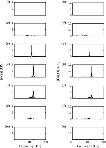
In figure 3 we can see the power spectra (FFT) corresponding to the time series of pressure and chemiluminesence fluctuations illustrated in figure 2. We observe that, as thermoacoustic instability is approached (figure 3, equivalence ratio
 $=$
0.68 and 0.50), the FFTs corresponding to both chemiluminesence and pressure fluctuations show peaks at a single frequency close to 120 Hz. This frequency varies slightly as the equivalence ratio is changed. This variation can be attributed to variation in the flame shape and flame dynamics at different equivalence ratios, leading to variation in local acoustic impedance and speed of sound along the length of the combustor. A detailed flame analysis is required to gain a thorough understanding of this observation. Such a study is outside the scope of the present paper. As the equivalence ratio is further reduced, the amplitude of the peak reduces (figure 3, equivalence ratio
 $=$
0.47). Close to blowout, the power spectrum does not contain any significant peak.
(a,c,e,g,i,k,m) FFTs corresponding to the pressure fluctuations in figure 2(a,c,e,g,i,k,m). (b,d,f,h,j,l,n) FFTs corresponding to chemiluminesence fluctuations in figure 2(b,d,f,h,j,l,n). Equivalence ratios are as in figure 2, i.e. 0.95 (a,b), 0.80 (c,d), 0.68 (e,f), 0.50 (g,h), 0.47 (i,j), 0.44 (k,l), 0.29 (m,n). We observe that in both pressure and chemiluminesence time series, as we approach thermoacoustic instability, there is growth of oscillations at a single frequency around 120 Hz (slight variations according to equivalence ratio). However, as we approach blowout, the oscillations at the dominant frequency die down.

(a) Variation in Hurst exponent,
 $H_{2}$
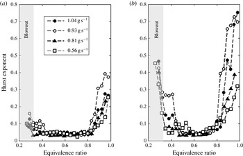
, estimated based on pressure fluctuations with respect to variation in equivalence ratio. (b) Variation in Hurst exponent estimated based on chemiluminescence with respect to variation in equivalence ratio. Note that the Hurst exponent reduces its value as we approach thermoacoustic instability and increases as we approach blowout. The Hurst exponent for this study is estimated from the time-series segments ranging from roughly two to four acoustic cycles.

Analysing the power spectra of the pressure and chemiluminesence fluctuations, we were not able to obtain any significant understanding regarding the complex dynamics exhibited by the pressure and chemiluminesence fluctuations. In the next section, we try to understand the complex behaviours in detail by studying the variation of the fractal characteristics of both chemiluminescence and pressure signals.
4.2. Scaling characteristics of the signals
In order to understand the scaling characteristics of the fluctuations in pressure and chemiluminescence signals, we estimate the Hurst exponent, a measure indicative of the fractal dimension of the time series. Figure 4(a) shows the variation of the Hurst exponent (
 $H_{2}$
, estimated from the pressure time series) with equivalence ratio as we approach blowout. The Hurst exponent for this study is estimated from the time-series segments ranging from roughly two to four acoustic cycles. With this choice of range of segment length, we can ensure that we identify the transition of the signal from aperiodic to periodic nature (Nair & Sujith Reference Nair and Sujith2014). If we include segments of length
 ${<}1$
acoustic cycle, we will be unable to capture the periodicity at the onset of thermoacoustic instability. However, for reliable results, the guideline says that the lower bound for the segment length should be two acoustic cycles (Ihlen Reference Ihlen2012; Nair & Sujith Reference Nair and Sujith2014) Also, if we were to include segments longer than four acoustic cycles, the fluctuations would be averaged out and we would lose the important information about the scaling characteristics of the signal on faster time scales. From previous studies, it has been observed that a range of scales of 2–4 acoustic cycles is optimal for our analysis (Nair & Sujith Reference Nair and Sujith2014). The time series used for the analysis is 3 s (30 000 data points) long.
Note that for all the different mass flow rates of fuel, the Hurst exponent approaches zero at the onset of thermoacoustic instability and increases to a higher value at blowout. As we approach thermoacoustic instability, the pressure signals become intermittent, with the region of periodicity getting longer (Nair et al.
Reference Nair, Thampi and Sujith2014), and at full-blown instability, the pressure signals are sinusoidal in nature (figure 2
a,c,e,g,i,k,m). Since sinusoidal signals are not fractal and have an integer fractal dimension (
 $D=2$
), the Hurst exponent (
 $H=2-D$
) for pressure signals during thermoacoustic instability is zero (Nair & Sujith Reference Nair and Sujith2014). As the equivalence ratio is reduced further from this point, the pressure fluctuation loses periodicity, and as a result, the Hurst exponent increases near blowout. This loss of periodicity of pressure fluctuations close to blowout could be attributed to the aperiodic flame extinction and reignition events that are present close to lean blowout. Such an aperiodic nature of flame extinction and reignition events prior to blowout was observed by Muruganandam (Reference Muruganandam2006) and Nair (Reference Nair2006). They observed that a burst of amplitude in the time series of acoustic pressure coincides with the spatially localized reignition events. Further, as the combustor approached flame blowout, they observed that the frequency of occurrence of aperiodic extinction and reignition events increased. This increase in aperiodic fluctuations near to blowout could be the reason why the Hurst exponent starts to increase close to blowout.
In a similar manner, figure 4(b) represents the Hurst exponents calculated from CH* chemiluminescence intensity measurements measured in sync with the pressure measurements used in figure 3(a,c,e,g,i,k,m). For chemiluminescence measurements, the variations in the Hurst exponent with equivalence ratio have characteristics similar to those exhibited by the Hurst exponents estimated from unsteady pressure measurements. That is, as we reduce the equivalence ratio from one, initially the Hurst exponent reduces due to increasing periodicity of the signals. Further, close to blowout, this periodicity is lost (figure 2) due to aperiodic flame fluctuations including extinction and reignition of the flame, and hence the Hurst exponent increases. However, in the case of chemiluminescence measurements, this increase is more pronounced than that exhibited by pressure measurements. Close to blowout, the chemiluminescence signals have Hurst exponent approaching a value of 0.5.
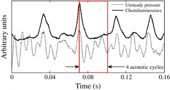
However, near the stoichiometric ratio of air–fuel mixture, the Hurst exponent obtained from the chemiluminescence signal has value greater than 0.5, indicating a persistent nature. A time series is called persistent if a large value is in general followed by a large value and a small value is followed by a small value (Kantelhardt Reference Kantelhardt and Meyers2011). Persistent signals have slowly evolving fluctuations (Ihlen Reference Ihlen2012). From figure 4, we can infer that, near the stoichiometric ratio of air–fuel mixture (
 ${\it\varphi}=0.96$
), the chemiluminescence signal has fluctuations with longer time scales than the signal for corresponding pressure fluctuations. Here it is evident that the chemiluminescence signal has slowly varying fluctuations compared to pressure fluctuations. It has been observed experimentally that flames can drive oscillations at frequencies corresponding to the subharmonics of the acoustic frequency (Bellows, Neumeier & Lieuwen Reference Bellows, Neumeier and Lieuwen2006). Such low-frequency oscillations could be the result of hydrodynamic fluctuations (Nair & Sujith Reference Nair and Sujith2015). As a result of this, for time-series segments of length 2–4 acoustic cycles (the highlighted part of figure 5), the chemiluminescence signal exhibits a persistent behaviour. Thus the Hurst exponent estimated based on chemiluminescence fluctuations for this operational condition has a value greater than 0.5.
Pressure and chemiluminescence fluctuations near stoichiometry
 $({\it\varphi}=0.96)$
for a fuel flow rate of
 $1.04~\text{g}~\text{s}^{-1}$
. Note that for two to four acoustic cycles, the chemiluminescence signal has persistent characteristics. This is because here the time scales associated with flame fluctuations are longer than acoustic time scales since flame fluctuations have a frequency subharmonic to the acoustic frequency.

In the previous paragraphs, we looked at the monofractal characteristics of pressure and chemiluminescence time series whereas, looking at the previous research (Nair & Sujith Reference Nair and Sujith2014), it is highly possible that the signals have multifractal characteristics. Hence, before drawing any conclusions, we need to study the multifractal characteristics of these fluctuations to obtain a better understanding of the scaling characteristics and the complex nature of the time series. In the following section we will analyse the multifractal characteristics of the unsteady pressure and CH* chemiluminescence time series.
4.3. Complexity in scaling: multifractality
The Hurst exponents plotted in figure 3 indicates the scaling laws corresponding to
 $H_{2}$
(Hurst exponent of order 2).
 $H_{2}$
alone represents only the scaling behaviour of the standard deviation of the fluctuations in time series. However, as explained in § 2, a time series can exhibit multifractal characteristics where the scaling behaviour depends upon the amplitude of the fluctuation. In other words, the scaling behaviour for central moments of fluctuations varies depending upon the order of the central moment. Already, it is established that turbulent flows have a multifractal scaling behaviour (Sreenivasan & Meneveau Reference Sreenivasan and Meneveau1986) arising from the underlying multiplicative process of Richardson’s energy cascade (Richardson Reference Richardson1922). Further, we know from recent research that combustion noise is amenable to a multifractal description (Nair & Sujith Reference Nair and Sujith2014). Considering these findings, in this section, we investigate the multifractal nature of pressure and chemiluminescence fluctuations from the bluff-body-stabilized combustor. In particular, we study the multifractal characteristics of the system close to blowout.
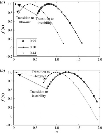
In figure 5, we can see that when the combustor is operated near the stoichiometric air–fuel ratio, the multifractal spectrum is broad. This indicates that the signal is multifractal and that there is an underlying multiplicative process in the system (Sreenivasan Reference Sreenivasan1991; Schertzer & Lovejoy Reference Schertzer and Lovejoy2011). As we increase the airflow rate and reach an equivalence ratio of 0.50, the combustor exhibits thermoacoustic instability. During thermoacoustic instability, both pressure and chemiluminescence signals are periodic and sinusoidal in nature. Here, since the fluctuations have a sinusoidal nature, the multifractal spectrum collapses and the Hurst exponents become near zero for all orders.
However, as we increase the airflow rate further, the equivalence ratio reduces and we approach blowout. Prior to blowout, the multifractal spectrum becomes broader than the multifractal spectra during thermoacoustic oscillations. This is because the signals prior to blowout are intermittent in nature with a multifractal structure to them (figure 4). It is to be noted that the multifractal spectrum is relatively narrower for the pressure signal for all equivalence ratios as compared to that of the corresponding chemiluminescence fluctuations. This is caused by the preferential amplification of pressure fluctuations close to the frequency corresponding to the fundamental acoustic frequency of the combustor, due to which the pressure fluctuations always tend to be relatively more periodic than the chemiluminescence fluctuations.
4.4. Approach to blowout in the absence of thermoacoustic instability
Until now, we have discussed the approach to blowout for a combustion system that exhibits thermoacoustic instability at lean equivalence ratios. Thermoacoustic instability can originate when the unsteady fluctuations in heat release rate couple with the acoustic field in the combustor, establishing a positive feedback between the acoustic and heat release fluctuations. Further, limit cycle oscillations are produced only if the acoustic energy added to the system is sufficiently high to balance the losses due to the damping present in the system. Hence a combustor might not exhibit thermoacoustic instability either when a positive feedback is not established, or when the acoustic energy added to the system is not adequate to compensate for the acoustic energy lost due to damping in the system. It is important that we study the blowout behaviour for such systems as well.
For this part of the study, we used the same combustor configuration as given in figure 1. We observe that this configuration of the combustor does not exhibit thermoacoustic instability at low fuel flow rates (
 ${<}0.4~\text{g}~\text{s}^{-1}$
) due to reduced amplitude of the fluctuations of heat release rate. Hence we study the dynamics of pressure and chemiluminescence oscillations at a fuel flow rate of
 $0.37~\text{g}~\text{s}^{-1}$
. The experiment is performed by varying the airflow rate from a value corresponding to an equivalence ratio of 0.98, in discrete steps, until the flame blowout happens. The data acquisition is done as described in § 3.
As we reduce the equivalence ratio from 0.98 in steps until blowout, the pressure and CH* chemiluminescence signals exhibit the following dynamics: low-amplitude aperiodic oscillations
 $\rightarrow$
intermittency
 $\rightarrow$
low-amplitude aperiodic oscillations
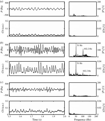
 $\rightarrow$
blowout. This sequence is illustrated in figure 6. At an equivalence ratio of 0.98, pressure and chemiluminescence signals have low amplitude and are aperiodic in nature. When the equivalence ratio is 0.67, the pressure and chemiluminescence signals exhibit intermittent oscillations where periodic fluctuations alternate with aperiodic fluctuations in an apparently random manner. Further, at an equivalence ratio of 0.38, both chemiluminescence and pressure fluctuations have low amplitude and are aperiodic.
Next, we analyse the multifractal characteristics of these oscillations. Figure 8 illustrates the variation of Hurst exponent
 $(H_{2})$
with equivalence ratio for a fixed fuel flow rate of
 $0.37~\text{g}~\text{s}^{-1}$
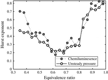
. We can see that, even in this case where the system is not exhibiting thermoacoustic instability, the Hurst exponent reduces in value as we approach lean equivalence ratios. For a lean equivalence ratio, unsteadiness in the flame causes the heat release rate to fluctuate. As these fluctuations are confined within an acoustic resonator (the combustor), the resonator preferentially amplifies the fluctuations at frequencies close to its natural frequencies (Chiu & Summerfield Reference Chiu and Summerfield1974; Strahle Reference Strahle1978; Hegde et al.
Reference Hegde, Reuter, Daniel and Zinn1987). However, since the fuel flow rate is low, the unsteady heat release rate is not adequate to drive the system to sustained limit-cycle oscillation. Nevertheless, as indicated before, in lean conditions, the signals exhibit intermittency where the signal switches from periodic to aperiodic fluctuations in an apparently random manner (figure 7
b). As a result of intermittent oscillations, there is an increased periodicity in the signals at lean equivalence ratios compared to that near stoichiometric equivalence ratios. However, since the system does not transition to full-blown instability, the Hurst exponent calculated from both pressure and chemiluminescence fluctuations decreases to a value close to 0.2 as opposed to a value near zero in a condition where the system exhibits full-blown instability. Further, near to blowout, the pressure and chemiluminescence fluctuations lose their periodic nature (figure 8) due to aperiodic flame extinction and reignition, resulting in an increase in Hurst exponent.
Another important aspect to be noted here is that the Hurst exponent estimated using both pressure and chemiluminescence time series has a value above 0.5 for equivalence ratios near to stoichiometry and near to blowout. As mentioned before, in this study, the Hurst exponent is estimated from the time-series segments ranging from roughly two to four acoustic cycles.
The multifractal spectrum for a bluff body combustor for three equivalence ratios (0.95, 0.50, 0.44) (a) estimated based on unsteady pressure time-series data and (b) estimated based on corresponding chemiluminescence time-series data. Here the fuel flow rate is
 $0.93~\text{g}~\text{s}^{-1}$
. In both cases, the width of the multifractal spectrum initially decreases as we approach the thermoacoustic instability and becomes close to zero at the instability. At leaner equivalence ratios, we do not have any thermoacoustic instability and we are closer to the blowout limit; here the multifractal spectrum width increases. The multifractal spectrum is estimated for
 $q$
ranging from
 $-2$
to 2.

The time series and corresponding power spectra for unsteady pressure and CH* chemiluminescence fluctuations for equivalence ratios of (a) 0.95 (
 $Re=0.44\times 10^{4}$
), (b) 0.67 (
 $Re=0.63\times 10^{4}$
) and (c) 0.38 (
 $Re=1.10\times 10^{4}$
). Note that the frequency corresponding to the acoustic mode (fundamental frequency) of the combustor is around 102.2 Hz. Near stoichiometry and near to blowout, neither pressure nor CH* chemiluminescence fluctuations have a major frequency component near the acoustic mode of the combustor. However, in between, at an equivalence ratio of 0.67, the pressure and CH* chemiluminescence fluctuations have a frequency component at the acoustic mode of the combustor. However, the dominant frequency is a subharmonic (51.0 Hz) of the frequency corresponding to the acoustic mode of the combustor (102.2 Hz). Further, pressure and chemiluminescence signals exhibit intermittency at an equivalence ratio of 0.67. The bin size in calculating the FFT was 0.3 Hz, and the time series used had 30 000 data points.

Variation of Hurst exponent with equivalence ratio. Here we can notice that, even though the system does not transition to thermoacoustic instability, the Hurst exponent (
 $H_{2}$
, estimated based on both pressure and chemiluminescence signals for time-series segments ranging from two to four acoustic cycles) reduces as we approach lean equivalence ratios and further increases close to blowout. Further, it should be noted that the Hurst exponents have values greater than 0.5 near stoichiometric equivalence ratios, indicating that for two to four acoustic cycles both pressure and chemiluminescence signals have persistent behaviour.

This implies that if we have a time series with dominant frequency much less than the acoustic frequency, the signal will largely have persistent characteristics for two to four acoustic cycles. The power spectrum corresponding to pressure and CH* chemiluminescence oscillations measured during combustion at near-stoichiometric equivalence ratio has a shallow peak at a frequency corresponding to the subharmonic of the acoustic frequency (figure 7 a). The presence of this dominant low-frequency (much lower than the acoustic frequency) component in the signal causes the estimated Hurst exponent to have a value greater than 0.5. The physical reason for presence of this subharmonic frequency requires further understanding of the flow physics and the flame dynamics in these experimental conditions and hence is beyond the scope of the present paper. At an equivalence ratio of 0.67, the oscillations exhibit a frequency component corresponding to the acoustic mode of the combustor. However, even in this case, the dominant frequency is the subharmonic (51 Hz) of the frequency of the acoustic mode (102.2 Hz) (Bellows et al. Reference Bellows, Neumeier and Lieuwen2006; Moeck et al. Reference Moeck, Oevermann, Klein, Paschereit and Schmidt2009).
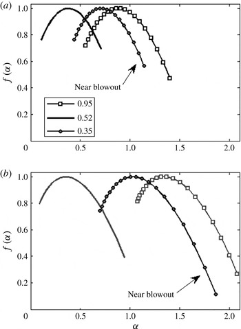
Figure 9 illustrates the variation in multifractal characteristics as we approach blowout. Here the multifractal spectrum does not shrink to a point as seen in figure 6. However, the spectrum width initially decreases as we reduce the equivalence ratio and increases close to blowout. This initial decrease can be attributed to the increase in periodicity of the time series for lean equivalence ratios, due to the appearance of intermittent periodic oscillations in lean conditions (figure 7 b). Further, the preferential amplification of the pressure fluctuations at frequencies close to the natural frequency of the combustor leads to an increased periodicity in the acoustic signals as compared to that of the chemiluminescence signals. As a result, the multifractal spectrum estimated from the acoustic signals is narrower than that estimated from chemiluminescence signals for all equivalence ratios (figure 9).
The multifractal spectra for a bluff-body combustor for three equivalence ratios (0.95, 0.52 and 0.35) are (a) estimated based on unsteady pressure time-series data and (b) estimated based on corresponding chemiluminescence time-series data. Here the fuel flow rate is
 $0.37~\text{g}~\text{s}^{-1}$
. In both cases, the multifractal spectrum width initially decreases as the equivalence ratio decreases. However, closer to the blowout limit, the multifractal spectrum width increases. The multifractal spectrum is estimated for
 $q$
ranging from
 $-2$
to 2.

From the analysis presented in this section, it is clear that even when the system does not transition to full-blown instability, through the presence of intermittency, the system dynamics are affected by the acoustic scales in the lean conditions. Since prior to blowout, we observe intermittency in the time series (figure 7 b), it is advisable to include the acoustic feedback mechanisms in models that predict blowout. Thus, while modelling the dynamics close to blowout, we need to consider the acoustic characteristics of the confinement (the combustor) to be able to capture the intermittent dynamics prior to blowout. Further, including the acoustic field in the model may be critical to getting accurate estimates of the stability margin for lean blowout.
Further, considering that blowout is indicated by an increase in Hurst exponent (in conjunction with a decrease in equivalence ratio), irrespective of whether or not the combustor exhibits thermoacoustic instability, we suggest that the Hurst exponent could be used as a precursor to detect an impending blowout (Unni, Nair & Sujith Reference Unni, Nair and Sujith2014). Since Nair & Sujith (Reference Nair and Sujith2014) have already shown that the Hurst exponent can be used as a precursor to instability (Hurst exponent approaching a value close to zero is indicative of the onset of instability), we conclude that Hurst exponent can be used as the single precursor that could detect both an impending blowout and an impending thermoacoustic instability.
5. Conclusions
In this work, we investigated the multifractal characteristics of CH* chemiluminescence fluctuations and pressure fluctuations measured from a turbulent combustor. It was observed that when the transition to blowout happens through thermoacoustic instability, the Hurst exponent (estimated from both CH* chemiluminescence signals and pressure signals) initially approaches close to zero at the thermoacoustic instability and then increases near blowout. Also, the multifractal spectrum (estimated from both CH* chemiluminescence signals and pressure signals), which is wide at near-stoichiometric combustion, shrinks to a point at the thermoacoustic instability and broadens close to blowout. Further, even in an alternative scenario when the transition from stoichiometric combustion to blowout occurred with the combustor not exhibiting thermoacoustic instability, we observed that the Hurst exponent (estimated from both CH* chemiluminescence signals and pressure signals) initially decreases and then increases close to blowout. However, in such a situation, the Hurst exponent does not reduce to a value close to zero. In a similar manner, here the multifractal spectrum width (estimated from both CH* chemiluminescence signals and pressure signals) reduces initially and then increases close to blowout. However, it does not shrink to a point as in the former case. The presence of intermittency prior to blowout in either case was suggested as the cause for these observed behaviours. Considering that the dynamics of oscillations prior to blowout was characterized by intermittency even in a case where the system did not exhibit thermoacoustic instability, we suggest that acoustic characteristics of the combustor should be included in models that describe the combustion dynamics close to blowout. The multifractal nature of the pressure and CH* chemiluminesence signals prior to blowout suggests the complexity in the scaling behaviour of these time series. Considering this complexity in dynamics prior to blowout, we provide a framework based on the multifractal characteristics of pressure and chemiluminescence fluctuations describing blowout as a dynamic instability. Further, within this framework, we suggest that when an increase in Hurst exponent is observed in conjunction with a decrease in equivalence ratio, we can identify that we are approaching an impending blowout. Thus, with this study, we were able to suggest a unified framework based on multifractality, within which we can analyse the dynamics of both thermoacoustic instability and blowout.
Acknowledgements
We are grateful to Professor W. Polifke and Mr T. Komarek of TU Munich, Germany for sharing the design of the combustor. We acknowledge the help from Dr K. P. Harikrishnan and Professor G. Ambika in obtaining the multifractal spectrum of the reconstructed phase space attractor. We gratefully acknowledge the suggestions from Dr V. Nair throughout the course of this work. We also thank Mr E. A. Gopalakrishnan and Ms M. Murugesan for all the discussions and the constructive criticisms that they provided. Finally, we thankfully acknowledge the help provided by Mr M. Dileesh, Mr K. Dileep, Mr P. K. Hashir and Mr N. B. George in acquiring the data presented in this work.
Appendix
In the paper, we used multifractal detrended fluctuation analysis (MFDFA) to analyse the fractal nature of pressure and chemiluminescence fluctuations. However, analysing the fractal nature of the attractors corresponding to the pressure fluctuations could also give some insights into the structure of the phase space attractor corresponding to the dynamics. In this Appendix, we will compare the multifractal spectrum corresponding to the phase space attractors reconstructed from a pressure time series obtained prior to blowout (equivalence ratio 0.27, in figure 2) and combustion noise close to stoichiometric combustion (equivalence ratio 0.95, in figure 2).
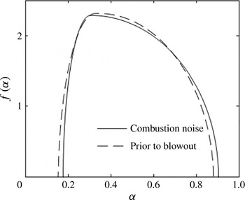
We use the method detailed by Harikrishnan et al. (Reference Harikrishnan, Misra, Ambika and Amritkar2010) to obtain the full multifractal spectrum representing the phase space attractor, see figure 10. We observe that the multifractal spectra corresponding to the two states are similar, suggesting that the multifractal characteristics are similar for both states. Thus this indicates that multifractal spectrum characteristics alone cannot distinguish between combustion noise and oscillations prior to blowout.
The multifractal spectra for combustion noise (equivalence ratio 0.95, in figure 2) and for a state prior to blowout (equivalence ratio 0.27, in figure 2). We can see that the two spectra are similar, indicating that phase space attractor for both combustion noise and the state prior to blowout have similar multifractal characteristics. Here the time series were embedded in three-dimensional phase space prior to the multifractal analysis.

We chose MFDFA over this method to analyse the multifractal characteristics since MFDFA is faster in terms of computation and can work with much shorter time series (details explained in § 2). Further, another aspect that needs to be highlighted here is that the phase space corresponding to the attractor has a high dimension close to blowout and during combustion noise. Hence, analysing the multifractality by reconstructing a phase space having a lower dimension (3 in this case, also in Gotoda et al. Reference Gotoda, Amano, Miyano, Ikawa, Maki and Tachibana2012) is disputable. However, embedding the time series in a high dimensional phase space increases the complexity in computation of the multifractal spectrum and hence makes this method unsuitable for any online precursor detection system.