







1. Introduction
A warm dense particle of non-volatile matter can float at the surface of a cooler but less dense liquid if the temperature difference exceeds the value needed for evaporation to produce a continuous film rather than individual bubbles. Because the film is thin in practice compared with the size of the particle, its presence causes the bulk meniscus to have an apparent contact line where the contact angle measured through the liquid has been increased from its static value to  ${\rm \pi}$ (Hendricks & Baumeister Reference Hendricks and Baumeister1971). The increase in contact angle increases the lift exerted by the liquid on the particle. As a result, a particle which would otherwise sink can remain suspended for as long as the film is present.
The duration of the phenomenon depends on the heat flow from the particle. The literature on vitrification of droplets of aqueous solution on liquid nitrogen contains two different treatments. Hendricks & Baumeister (Reference Hendricks and Baumeister1971) and Adda-Bedia et al. (Reference Adda-Bedia, Kumar, Lechenault, Moulinet, Schillaci and Vella2016) model the vapour film as a squeeze flow between two concentric spheres. Because the shape of the interface between the film and pool is prescribed, the balance of normal stress is not satisfied. The thickness of the film and the pressure distribution within it are determined using the Reynolds equation, the conduction equation and the force balance on the sphere. Song et al. (Reference Song, Adler, Xu, Kayaalp, Nureddin, Anchan, Maas and Demirci2010), by contrast, apply existing theory for film boiling on a sphere (Frederking & Clark Reference Frederking and Clark1963; Carey Reference Carey1992, p. 275). In it, flow within the film is assumed to be driven by the pressure gradient within the pool, as in the free convection boundary layer in a single phase; this analogy holds if the drops are large enough for surface tension to be negligible in the balance of normal stress. For the experiments performed by Song et al. on freezing drops of an aqueous solution on liquid nitrogen, drop radii range from  ${\sim }80\,\mathrm {\mu }{\rm m}$ to
 ${\sim }1$ mm; because the capillary length of liquid nitrogen is
 ${\sim }1$ mm, it is not obvious that surface tension should be negligible.
Numerical simulations by Maquet et al. (Reference Maquet, Sobac, Darbois-Texier, Duchesne, Brandenbourger, Rednikov, Colinet and Dorbolo2016) of their own experiments satisfy all relevant governing equations and boundary conditions. Their figure 5 shows film profiles calculated for the Leidenfrost flow between a volatile drop and a non-volatile pool of denser liquid. Because the density ratio is fixed in those calculations, the deflexion of the pool surface increases with drop size. Though the film structure evolves with drop size, those simulations do not determine whether the change in structure is a result of increasing deflexion, or of something else. The behaviour of volatile drops large compared with the capillary length is analysed by van Limbeek et al. (Reference van Limbeek, Sobac, Rednikov, Colinet and Snoeijer2019). Motion in the film is proved to be driven by the pressure gradient within the underlying liquid. Film structure and thickness are determined but no result is given for the total heat flow.
Here, the first systematic calculation is made to determine the Nusselt number for steady axisymmetric Leidenfrost flow between a rigid sphere of radius  $b$ and density
 $\rho _s$, and a pool of liquid of density
 $\rho _\ell$. Results are given only for a drop sufficiently small for the pressure gradient imposed by the underlying liquid to be negligible compared with the gradient in capillary pressure.
In § 2, the boundary value problem is posed for a sphere of arbitrary radius. This problem contains five parameters:
 \begin{equation} Pr=\frac{\mu c_p}{k}, \quad Bo =\frac{\rho_\ell g b^2}{\gamma}, \quad Cr= \frac{\mu {\kappa}}{\gamma b}, \quad D=\frac{\rho_s}{\rho_\ell}, \quad Ja=\frac{c_p\Delta T}{H_\ell^v}. \end{equation}
Symbols without a subscript  $\ell$ or
 $s$ refer to the vapour;
 $k=\rho c_p{\kappa }$ and
 $H_\ell ^v$ denote its thermal conductivity and the enthalpy of evaporation. The Prandtl number
 $Pr$ is about one. The sphere is denser than the liquid:
 $D>1$. For a sphere of radius
 $1$ mm at
 $293$ K on liquid nitrogen at its normal boiling point of
 $77.355$ K, the crispation number
 $Cr= 0.8\times 10^{-6}$, Jakob number
 $Ja= 1.2$ and
 $Bo=0.9$. (Though
 $Bo$ is often called the Bond number, in Bashforth & Adams (Reference Bashforth and Adams1883, p. 15), the same group appears (as their
 $\beta$) in an early example of a dimensionless boundary value problem. Bond was born in 1897.) Properties were obtained using the site at https://webbook.nist.gov; other than surface tension
 $\gamma$, they were evaluated at the mean temperature of
 $185$ K. Because the characteristic film thickness
 $h_0\to 0$ as
 $Cr\to 0$, the boundary-layer approximation is made following the initial formulation of the problem.
At the end of § 2, it is shown that in a film covering an  $O(1)$ fraction of the sphere, the motion is driven by the pressure gradient imposed by underlying liquid if
 $Bo\gg h_0$. In the other extreme
 $Bo\ll h_0$, the imposed pressure gradient is negligible; this limit is analysed here. Jones & Wilson (Reference Jones and Wilson1978) give an equivalent criterion for the isothermal flow in the gas film beneath a sphere settling onto a pool.
In § 3, the problem is simplified by assuming creeping flow. The convective nonlinearity in the energy equation is retained, however. The simplified equations admit a similarity solution determining the temperature profile across the film, and providing a pair of coupled ordinary differential equations determining the streamwise evolution of the pressure  $p$ and volume flow rate
 $q$ within the film in terms of film thickness
 $h$. The similarity solution allows the effect of the convective nonlinearity in the energy equation to be described completely by a modified form of the crispation number
 $Cr$. The method used to compute the Nusselt number is also outlined in this section.
Section 4 contains the main results of the numerical solutions. In addition to determining the Nusselt number, these solutions show how the solution evolves as the weight of the sphere is increased from an initial small value for which the interface is nearly plane. The film profile eventually assumes the form of a spherical bubble cap bounded by an apparent contact region. This structure is analysed in the rest of the paper.
The chief properties of the bubble cap are given in § 5. The boundary value problem for the contact region is derived in § 6, then in § 7 transformed into a simpler form and solved by a series expansion in powers of a parameter  $\lambda$ representing the strength of evaporation in the contact region. The expansion is carried out to
 $O(\lambda ^3)$. Section 8 contains the results for the apparent contact angle
 $\chi$ for the bubble cap and for the total evaporation. In § 9, these predictions are compared with numerical results. Conclusions are given in § 10.
Appendix A contains the forms of the Laplace relation used here; Appendix B, the similarity solution; Appendix C, the theory used to calculate the Nusselt number; Appendix D, the explicit solutions used in §§ 7 and 8; and Appendix E, the analysis used in the discussion of the numerical results in § 4.
Jones & Wilson (Reference Jones and Wilson1978), Duchemin, Lister & Lange (Reference Duchemin, Lister and Lange2005), Snoeijer, Brunet & Eggers (Reference Snoeijer, Brunet and Eggers2009) and Sobac et al. (Reference Sobac, Rednikov, Dorbolo and Colinet2014) describe analyses similar to that given here in §§ 5 and 6. Only that of Sobac et al. involves evaporation from the film and its contact region. In that analysis, and in this one, evaporation from the contact region is negligible to a first approximation. Including evaporation from the contact region in subsequent approximations reduces  $\chi$. By reducing the thickness of the main film, evaporation form the contact region therefore has a significant effect on the total evaporation rate. Though Sobac et al. (Reference Sobac, Rednikov, Dorbolo and Colinet2014) calculate the first correction to
 $\chi$, they neither comment on this effect nor demonstrate its importance for the total evaporation.
2. Governing equations
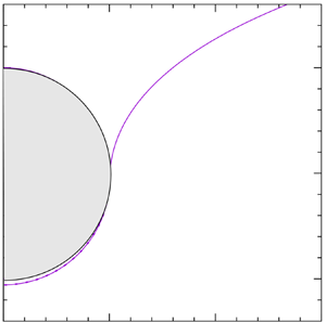
Figure 1 shows the geometry of the problem. The liquid is isothermal at the saturation temperature  $T_{\ell v}$; pressure within it is hydrostatic. The sphere is at uniform temperature
 $T_{\ell v}+\Delta T$. Arc length along the interface to point
 $P$ is denoted by
 $s$;
 $\boldsymbol {r}(s)$ denotes the position vector
 $CP$ of
 $P$ relative to the centre
 $C$ of the sphere. The thickness of the vapour film
 $h(s)=r(s)-b$; as shown in the figure,
 $h_0=h(0)$. The unit normal
 ${\boldsymbol n}$ to the interface points into the liquid; it has Cartesian components
 $n_i$. The origin
 $O$ for the cylindrical coordinates
 $\{{\sigma }, z\}$ is at the level of the flat interface at infinity. The inset shows the relation between
 ${\rm d}s$,
 ${\rm d} {\sigma }$,
 ${\rm d} z$ and the inclination
 $\alpha$, i.e. the angle between the tangent to the interface and the horizontal. The force exerted by the sphere on the liquid is denoted by
 $-2{\rm \pi} F{\boldsymbol e}_z$. (The sphere is assumed to be stationary, and the solution to be axisymmetric. Adda-Bedia et al. (Reference Adda-Bedia, Kumar, Lechenault, Moulinet, Schillaci and Vella2016, p. 1080) show by experiment that the particle in fact translates and the flow is not axisymmetric.) The body force is negligible within the vapour but not (in general) within the liquid (
 $\rho \ll \rho _\ell$).
Cylindrical coordinates  $({\sigma },z)$,
 $z=0$ on the flat interface. Sphere: centre
 $C$ at
 $z=c$. Liquid–vapour interface:
 $s= |LP|$, arc length from the lowest point
 $L$ to point
 $P$;
 ${\boldsymbol r}(s)= CP$, position vector of point
 $P$. Vapour layer: thickness
 $h=|{{\boldsymbol r}}|-b$, pressure
 $p$;
 $h_0$,
 $p_0$, values at
 $s={\theta }=0$. Inset: unit normal
 ${\boldsymbol n}$; tangent
 ${\rm d}\boldsymbol {r}$, inclination
 $\alpha$;
 ${\rm d} s=|{\rm d} {\boldsymbol r}|$.

Dimensionless variables (without asterisks) are based on the primary quantities  $b$,
 $\gamma /b$,
 $\Delta T$ and the scale
 ${\kappa } Ja/b$ imposed by the balance of energy at the interface:
 \begin{equation} {\boldsymbol r}_*=b{\boldsymbol r}, \quad {\boldsymbol v}_*= \frac{{\kappa} Ja}{b}{\boldsymbol v}, \quad p_*-p_{*a}=\frac{\gamma}{b}p, \quad T_*=T_{\ell v}+ T \Delta T. \end{equation}
Within the vapour
 \begin{gather} \mbox{div }{\boldsymbol v}=0, \end{gather}
 \begin{gather} Pr^{{-}1}Ja^2 {\boldsymbol v} \boldsymbol{{\cdot}} \boldsymbol{\nabla}{\boldsymbol v} ={-}Cr^{{-}1} \boldsymbol{\nabla}p+Ja{\nabla}^2{\boldsymbol v}, \end{gather}
 \begin{gather} Ja\,{\boldsymbol v}\boldsymbol{{\cdot}} \boldsymbol{\nabla}T= {\nabla}^2 T, \end{gather}
so that heat is transferred by pure conduction if  $Ja\ll 1$.
On the sphere
 \begin{equation} {\boldsymbol v}=0, \quad T=1. \end{equation}
On the liquid–vapour interface
 \begin{gather} T=0= {\boldsymbol n}\boldsymbol{{\cdot}}( {\boldsymbol v} -\boldsymbol{\nabla}T), \end{gather}
 \begin{gather} p+Bo\, z =\mbox{div }{\boldsymbol n} +Ja\,Cr\, {\sigma}'_{ij} n_in_j, \end{gather}
 \begin{gather} {\sigma}'_{ij} n_j - ({\sigma}'_{kl} n_kn_l) n_i=0; \end{gather}
the deviatoric stress tensor  $\sigma '_{ij}={\sigma }_{ij}+p\,\delta _{ij}$, stress tensor
 $\sigma _{ij}$. Equation (2.2g) is a simplified form of the balance of total energy at the interface. The body force enters only through the boundary condition (2.2h).
As stated by (2.2h) and (2.2i), the liquid is assumed to exert only a hydrostatic pressure  $-Bo\,z$ on the phase interface. This assumption is explained next. Motion in the liquid consists of a primary flow required by continuity of the component of
 $\boldsymbol {v}$ along the interface and a weaker secondary flow required by continuity of the mass flux
 $\rho \boldsymbol {v}\boldsymbol {{\cdot }} \boldsymbol {n}$. The shear stress exerted by the liquid can be negligible, or not, depending on the magnitude of the parameter
 $\mathscr {M}= \mu b/(\mu _\ell h_0)$. For
 $\mathscr {M}\to \infty$, the characteristic shear stress in the vapour is large compared with that in the liquid; continuity of the shear stress then requires the shear stress to vanish in the vapour at the interface. Similarly, for
 $\mathscr {M}\to 0$, the tangential component of
 $\boldsymbol {v}$ vanishes in the vapour at the interface. Jones & Wilson (Reference Jones and Wilson1978, p. 269) assume the former; Hendricks & Baumeister (Reference Hendricks and Baumeister1971, table 1) and van Limbeek et al. (Reference van Limbeek, Sobac, Rednikov, Colinet and Snoeijer2019, p. 1161) assume the latter. Following (4.4), it is shown that within the lubrication approximation, the choice of boundary condition amounts to modifying the value used for
 $Cr$.
For the sphere to be in equilibrium,
 \begin{equation} F=\tfrac{2}{3} D\,Bo= \int_0^{\rm \pi} p\cos{\theta}\,\sin{\theta}\, {{\rm d} {\theta}} + Ja\,Cr\int_0^{\rm \pi} ({\sigma}'_{r{\theta}}\sin{\theta}-{\sigma}'_{rr}\cos{\theta})\,\sin{\theta}\,{\rm d}{\theta}. \end{equation}
At  $s=0$, pressure
 $p_0$ and film thickness
 $h_0$ are to be determined as part of the solution. The outer boundary conditions are
 \begin{equation} \mbox{ as } h/h_0\to \infty, \quad p/p_0\to 0;\quad \mbox{as } s\to \infty, \quad z\to 0. \end{equation}
Condition (2.4a) is stated in terms of  $h$ rather than
 $s$ because the structure of the film determines the value of
 $s$ at which
 $p/p_0\to 0$. The problem so defined determines
 $h_0$,
 $p_0$ and the ordinate
 $c$ of the centre of the sphere as functions of
 $Bo$,
 $Ja$,
 $Pr$,
 $Cr$ and
 $F$.
Next, it shown that when the film covers a fraction  $\sim 1$ of the surface of the sphere, motion within the film is driven by the gradient in capillary pressure if
 $Bo\ll h_0$; conversely, it is driven by the pressure gradient imposed by the underlying liquid if
 $Bo\gg h_0$.
In the boundary-layer approximation, the momentum equation is
 \begin{equation} Pr^{{-}1}Ja^2
{\boldsymbol v} \boldsymbol{{\cdot}}
\boldsymbol{\nabla}{v}_\theta
={-}Cr^{{-}1}\frac{{\rm d} p}{{\rm d} {\theta}} + Ja
\frac{{\partial}^2
v_{\theta}}{{\partial}{\theta}^2}.
\end{equation}
In this approximation  $p$ is uniform across the thin film. It is determined by (2.2h), which with error
 $O(h_0^2)$ is
 \begin{equation}
p= Bo\{(1+h)\cos{\theta} -c\} + 2- 2h -\frac{1}{\sin{\theta}}\frac{{\rm d}}{{\rm d}{\theta}}
\left(\sin{\theta}\frac{{\rm d} h}{{\rm d}
{\theta}}\right). \end{equation}
The term in braces represents the pressure imposed by the underlying liquid; remaining terms represent the capillary pressure. As noted by Jones & Wilson (Reference Jones and Wilson1978), there are two extremes. For  $Bo\gg h_0$, the pressure gradient is given by
 ${\rm d} p/{\rm d}{\theta } =-Bo\,\sin {\theta }$, except within the contact region: the motion in the main film is then driven by the pressure gradient imposed by the underlying liquid. Conversely, for
 $Bo\ll h_0$ the pressure gradient within the film is equal to the gradient in capillary pressure. (Because
 $h_0$ is a flow property, it has different values in the two inequalities.) This condition for the gradient in hydrostatic pressure to be negligible is more demanding than the condition
 $Bo\ll 1$ required for the hydrostatic pressure itself to be negligible in the force balance on the sphere. Brandão & Schnitzer (Reference Brandão and Schnitzer2022, p. 1121) analyse the behaviour of the film assuming
 $D$ to be fixed and
 $Bo\to 0$. Consequently,
 $F\ll 1$ and the film covers only a vanishingly small part of the sphere. As a result, their analysis is only indirectly related to the argument of Jones & Wilson (Reference Jones and Wilson1978) just summarized.
The scaling  $Ja/Pr$ for the ratio of inertial to viscous terms is not an artefact of a particular choice of scales. Within the main film where the dimensional radial velocity
 $v_r^*$ is determined by the balance of total energy at the interface, the product of dimensional film thickness
 $h^*$ with
 $v_r^*$ depends only on
 ${\kappa }$ and
 $Ja$:
 $h^* v_r^*\sim {\kappa }\, Ja$ and the ratio of inertial to viscous terms is
 $\rho h^*v_r^*/\mu \sim Ja/Pr$. Within the contact region, the velocity is, however, determined instead by the total evaporation from the main film; this will slightly increase the effect of inertia there. Despite this, fluid inertia is assumed to be negligible in the rest of this work. The convective nonlinearity in the energy equation is retained, however.
3. Specialization to quasi-parallel creeping flow
The coupled energy and momentum equations now admit a similarity solution including convective heat transport (Appendix B). In addition to determining the profiles of velocity and temperature, it provides two equations relating the streamwise evolution of  $p({\theta })$ and
 $q=\psi (1+h,{\theta })$ (Stokes streamfunction
 $\psi$) to the unknown film thickness
 $h({\theta })$. (The volume flow rate is given by
 $2{\rm \pi} q$.)
3.1. Chief properties of the similarity solution
The equations for  $p$ and
 $q$ are
 \begin{equation} \frac{h }{\sin{\theta}}\frac{{\rm d} q}{{\rm d} {\theta}}={\varGamma}(Ja),\quad \frac{h^3\sin{\theta}}{ Ja\,Cr q} \frac{{\rm d} p}{{\rm d} {\theta}}={-}c. \end{equation}
The constant  $c$ depends on the boundary condition for
 $v_{\theta }$ at the interface. For
 $ {\partial } v_{\theta }/ {\partial } r|_{1+h}=0$, as assumed here,
 $c=3$. For
 $v_{\theta }(1+h\,{\theta })=0$,
 $c=12$.
The function  ${\varGamma }(Ja)$ is the product of film thickness with the heat flux into the vapour–liquid interface:
 \begin{equation} {\varGamma}(Ja)=\left. -h \frac{{\partial} T}{{\partial} r}\right|_{1+h}. \end{equation}
This function is given by (B9); it describes completely, and without approximation, the effect of convective transport of heat.
Figure 2 shows  ${\varGamma }$ as a function of
 $Ja$. In the limit as
 $Ja\to 0$,
 ${\varGamma }\to 1$ because the left-hand side of (2.2c) then vanishes and, in the thin-film approximation,
 $T$ varies linearly across the film. For
 $Ja>0$,
 ${\varGamma }<1$ because vapour flows from the interface towards the sphere: this motion reduces the temperature gradient at the liquid–vapour interface but steepens that at the sphere. The corresponding difference between the heat fluxes is transported downstream. The choice of
 $c$ has only a modest effect on either flux.
Product of film thickness and heat flux as given by the similarity solution (B9). Solid and broken curves show the effect of the boundary condition on  $v_{\theta }$ at the vapour side of the interface: solid curves,
 $ {\partial } v_{\theta }/ {\partial } r=0$ (
 $c=3$); broken curves,
 $v_{\theta }=0$ (
 $c=12$). Short curves, Taylor series (B11) to
 $O(Ja^2)$.

The form of (3.1a) and (3.1b) reflects the choice of  $b$,
 $Ja\,{\kappa }/b$ and
 $\gamma /b$ as scales for length, velocity and pressure. If instead,
 ${\varGamma }\,Ja\,{\kappa }/b$ is used as the scale for velocity, with no other change,
 $q$ is replaced by
 ${\varGamma } q$, and the pair of equations contains only the single parameter
 ${\varGamma }\,Ja\,Cr$. The effect of convective transport of heat is therefore equivalent to that of reducing
 $Cr$ by the factor
 ${\varGamma }(Ja)$. With this understanding,
 ${\varGamma }$ is set to unity.
3.2. The boundary value problem for  $Bo\ll h_0$

The Laplace relation provides the equation needed to complete the system. In the form given as (A2) it is expressed using arc length  $s$ along the liquid–vapour interface. Without approximation, (3.1a) and (3.1b) are therefore expressed in terms of
 $s$ by multiplying throughout
 ${\rm d} {\theta }/{\rm d} s$.
With  ${\sigma }=(1+h)\sin {\theta }$ denoting the cylindrical coordinate of a point
 $s$ on the interface,
 ${\theta }$ its spherical coordinate and
 $\alpha$ the inclination (figure 1), the five dependent variables
 $\alpha$,
 $h$,
 ${\theta }$,
 $p$ and
 $q$ satisfy the following problem.
For  $0< s<\infty$,
 \begin{gather} -{\frac{1}{3}} h^3\sin{\theta}\frac{{\rm d} p}{{\rm d} s}= Ja\,Cr \,q\,\frac{{\rm d} {\theta}}{{\rm d} s}, \end{gather}
 \begin{gather} \frac{h }{\sin{\theta}}\frac{{\rm d} q}{{\rm d} s}= \frac{{\rm d} {\theta}}{{\rm d} s}, \end{gather}
 \begin{gather} \frac{{\rm d} \alpha}{{\rm d} s}+\frac{\sin\alpha}{{\sigma}} =p, \end{gather}
 \begin{gather} \frac{{\rm d} h}{{\rm d} s} =\sin({\theta}-\alpha), \end{gather}
 \begin{gather} \frac{{\rm d} \theta}{{\rm d} s}= \frac{\cos({\theta}-\alpha)}{1+h}. \end{gather}
The geometric identities (3.3d) and (3.3e) are derived in Appendix C. According to these identities  $h$ is a decreasing function of
 $s$ if the inclination
 $\alpha$ of the interface exceeds that of the tangent to the sphere; and
 ${\rm d} {\theta }/{\rm d} s \gtrless 0$ according as
 $\alpha \gtrless {\theta } -{\textstyle \frac {1}{2}}{\rm \pi}$:
 ${\theta }$ increases with
 $s$ until the radius vector becomes tangent to the interface, but decreases thereafter.
The boundary conditions are
 \begin{equation} 0={\theta}=\alpha=q, \quad h=h_0, \quad p=p_0 \end{equation}
at  $s=0$; and
 \begin{equation} p/p_0\to 0 \end{equation}
as  $h/h_0\to \infty$.
Because  $Bo$ does not enter into the system (3.3), its solution is decoupled from the interface displacement. It is now convenient to choose the origin for
 $z$ to be at the centre
 $C$ of the sphere (rather than at the level of the flat interface at infinity, as in figure 1). With this choice, the cylindrical coordinates of a point on the interface are given by
 \begin{equation} {\sigma}=(1+h)\sin{\theta},\quad z={-}(1+h)\cos{\theta}. \end{equation}
For ease of reference, the relation for  ${\sigma }$ given above (3.3) is repeated as (3.5a).
Although  $Bo$ does not enter into (3.3), it still enters into the force balance (2.3) but only as part of the group
 $F= \tfrac {2}{3}Bo\,D$. The solution of (3.3) satisfying the boundary conditions therefore depends on only two parameters,
 $Ja\,Cr$ and
 $F$, rather than all five listed as (1.1a–e). (In effect, except where
 $g$ is multiplied by the density
 $\rho _s$ of the sphere, gravity is taken as negligible for the analysis in this paper.)
The system (3.3) admits a solution such that in the limit as  $s\to \infty$,
 $p=o(s^{-3})$,
 $\alpha \to 0$,
 ${\theta }\to {\textstyle \frac {1}{2}}{\rm \pi}$,
 $h=O(s)$ and
 ${\rm d} q/{\rm d} s = o(s^{-2})$. The outer boundary (3.4 f) is therefore satisfied, and
 $q$ approaches a limiting value,
 $q_\infty$ (say). However, in the limit as
 $s\to \infty$,
 $h=O(s)$ so that the thin-film approximation underlying (3.1a,b) is no longer valid. Despite this, the limiting value
 $q_\infty$ can be interpreted once it is understood that in the limit as
 $Ja\,Cr\to 0$, the solution of (3.3) has an inner-and-outer structure.
The inner region consists of the thin film and its contact region. The outer limit is defined as  $Ja\,Cr\to 0$ (fixed
 $h$). In this limit,
 $h=O(1)$, and the Reynolds equation (3.3a) becomes
 \begin{equation} \frac{{\rm d} p}{{\rm d} s}=0, \quad \Rightarrow \quad p=0, \end{equation}
where the outer boundary condition (3.4 f) has been imposed. From (3.6b), it follows that the outer limit describes the bulk meniscus extending from the apparent contact circle to infinity. Because the reduced heat equation (3.3b) does not contain the small parameter  $Ja\,Cr$, the contribution of the outer region to the total evaporation is
 $O(1)$, i.e. independent of
 $Ja\,Cr$ in the limit. Provided the limiting value
 $q_\infty \gg 1$, the contribution from the outer region is therefore negligible. Values for
 $Nu$ obtained from the numerical solution therefore have a relative error
 $O(Nu^{-1})$. All other properties of the numerical solution are limited only by the precision of the numerical integration.
The outer solution for  $h$ has an apparent contact circle at which
 $h\to 0$ and
 $q\to \infty$. To demonstrate that this contact singularity is resolved by accounting for the thin film, Appendix C contains an example in which the outer solution for
 $q$ is obtained explicitly and matched to that for the thin film.
The numerical solution of (3.3) was obtained in parametric form. The program consists of three nested do loops. First, with  $Ja\,Cr$ fixed, the innermost loop integrates the system (3.3) from
 $s=0$ to a large value
 $s_1$ for a given pair
 $\{h_0,p_0\}$: this determines
 $p(s_1)$ for the pair
 $\{h_0, p_0\}$. Second, the intermediate loop imposes the condition
 $p_1(h_0,p_0)=0$ iteratively using Newton's method: this determines
 $p_0$ in terms of
 $h_0$. In this loop,
 $F$ is also obtained using the relation
 \begin{equation} \int_0^{s_1} (p-p_1){\sigma}\frac{{\rm d} {\sigma}}{{\rm d} s}\,{\rm d} s= \left. \left\{ {\sigma}\,\sin\alpha- {\frac{1}{2}} p{\sigma}^2\right\}\right|_{s={s_1}}= F. \end{equation}
(It follows by integrating the Laplace relation in the form (A1).) The result of the intermediate do loop is a triplet  $\{p_0, h_0, F\}$ satisfying (3.4 f) for the fixed value of
 $Ja\,Cr$. Third, the outer loop uses continuation to vary one of either
 $p_0$ or
 $h_0$: this generates the graphs of
 $p_0(F, Ja\,Cr)$ and
 $h_0(F,Ja\,Cr)$ given as the next figure.
The solution of (3.3) depends on only two parameters: in this work  $Ja\,Cr$ and
 $F$ are chosen.
4. Results from numerical solutions of (3.3)
4.1. Response curves
In figure 3(a,b), broken curves show values of  $p_0$ and
 $h_0/(Ja\,Cr)^{1/3}$ obtained from the numerical solution of (3.3) graphed against
 $F/(Ja\,Cr)^{1/3}$. With this choice of independent variable, results for different values of
 $Ja\,Cr$ form a single curve on the left-hand side of each panel. Each broken curve consists of two branches; the tangent to each curve becomes vertical at the branch point. In each panel, a single solid curve shows corresponding values obtained by solving the simplified system given in Appendix E; it describes the solution in the limit as
 $Ja\,Cr\to$ (fixed
 $F/(Ja\,Cr)^{1/3}$). Unlike the broken curves, the solid curve has no branch point: instead, it defines
 $h_0/(Ja\,Cr)^{1/3}$ and
 $p_0$ as single-valued functions of
 $F/(Ja\,Cr)^{1/3}$. Broken curves coincide with the solid curve for fixed
 $F/(Ja\,Cr)^{1/3}$; as
 $Ja\,Cr$ is reduced, broken and solid curves coincide over an increasing range. For
 $F/(Ja\,Cr)^{1/3} \to \infty$, the solid curve for
 $p_0$ approaches the asymptote
 $p_0=2$.
(a) Pressure and (b) film thickness at the stagnation point at  ${\theta }=0$. Broken curves, numerical solution of (3.3) for the values of
 $-\log _{10}(Ja\,Cr)$ indicated by the labels. Broken curves have two branches; as indicated by the dotted horizontal line in (a), the branch point occurs asymptotically at
 $p_0=2$. Solid curve, solution of the simplified system (E2) describing the limit
 $Ja\,Cr\to 0$ (fixed
 $F/(Ja\,Cr)^{1/3}$).

The overall behaviour of the solution of (3.3) is determined by the presence of the maximum in  $p_0$ (figure 3a). According to the solution of (E3), this maximum occurs when
 \begin{equation} F= 10.23(Ja\,Cr)^{1/3}; \quad \mbox{ then } \ h_0= 1.771\,(Ja\,Cr)^{1/3}, \quad p_0=2.4396. \end{equation}
The maximum value of  $p_0$ is only about
 $20\,\%$ greater than the pressure within a spherical bubble of unit radius. Once established, (4.1) was used to provide initial values for the method of continuation.
Because the maximum pressure exceeds 2, there are two values of  $F/(Ja\,Cr)^{1/3}$ for which
 $p_0=2$. The smaller value occurs on the left-hand side of the figure where the broken and solid curves coincide. According to the solution of (E3), for
 $p_0=2$,
 \begin{equation} F= 2.282 (Ja\,Cr)^{1/3}, \quad h_0= 1.021 (Ja\,Cr)^{1/3}. \end{equation}
To the left of this point in figure 3(a),  $h$ has a minimum at
 $s=0$ and increases monotonically with
 $s$; to the right of it,
 $h$ has instead a local maximum at
 $s=0$. In the form (A3), the Laplace relation determines the location
 $r({\theta })=1+h({\theta })$ of the interface in spherical coordinates. By evaluating it at
 ${\theta }=0$,
 \begin{equation} \left. r_{{\theta}{\theta}}\right|_0= {\textstyle\frac{1}{2}} r_0^2\left(2r_0^{{-}1}-p_0\right). \end{equation}
Consequently,  $h$ has a minimum at
 ${\theta }=0$ if
 $p_0$ is less than the pressure
 $2/r_0$ within a spherical bubble of radius
 $r_0$; a maximum otherwise. In the limit as
 $Ja\,Cr\to 0$,
 $r_0\to 1$ and
 $r_{{\theta }{\theta }}$ changes sign when
 $p_0\to 2$. As
 $F$ is increased from zero, the critical condition is necessarily first satisfied on the left-hand side of the pressure maximum.
Once the local maximum in  $h$ has formed, it is necessarily paired with a local minimum for
 $s>0$. Indeed,
 ${\rm d} h/{\rm d} s$ must then have two zeros because it is negative immediately beyond the maximum, but subsequently becomes positive because
 $r\to \infty$ as
 $s\to \infty$. As
 $F/(Ja\,Cr)^{1/3}$ is increased above the value (4.2a), the ratio of
 $h_0$ to the minimum increases. This leads to formation of a bubble cap and its contact ring.
Formation of the paired maximum and minimum can also be explained physically. Because the film is thin, the capillary pressure cannot exceed a value of the order of unity. Consequently, as the weight of the sphere is increased, the force balance on the sphere can be satisfied only if the capillary pressure acts on an increasing area. This requires that the film increase in length. However, for vapour to flow along the film, the capillary pressure must decrease with increasing  ${\theta }$. By itself, the increase in film length required by the force balance tends to decrease the magnitude of
 ${\rm d}^2 h/{\rm d}{\theta }^2$. This effect can be compensated if
 ${\rm d}^2h/{\rm d}{\theta }^2$ changes sign from negative to positive somewhere along the length of the film. Film profiles shown below illustrate this effect.
The weight of the heaviest sphere supportable by surface tension alone is determined by the point where the tangent to a broken curve in figure 3(a) becomes vertical. In the limit as  $Ja\,Cr\to 0$,
 $p_0\to 2$ at this point and
 $F\to 1$. As
 $p_0$ falls below 2 on the lower branch of the pressure curve,
 $r_0$ increases so that
 $r_{{\theta }{\theta }}|_0$ remains negative, as it must for the bubble cap to remain present. This increase in film thickness is evident in figure 3(b).
4.2. Film profiles
Figure 4 shows profiles obtained from the numerical solution of (3.3). As stated above (3.5), in the rest of this paper, the origin for  $z$ is taken to be at the centre of the sphere.
Interface profiles for  $Ja\,Cr= 10^{-8}$ and values of
 $p_0$ at, or to the right of, the maximum in figure 3(a): (a)
 $p_0=2.4311$ (
 $F/(Ja\,Cr)^{1/3}= 10.24$), inset showing the local minimum in
 $h$; (b)
 $p_0= 2.35$ (
 $F/(Ja\,Cr)^{1/3}= 28.78$), inset showing the spherical cap used to determine the contact angle
 $\chi$; (c)
 $p_0=2.0$ (
 $F/(Ja\,Cr)^{1/3}=464.1$); and (d)
 $p_0=1.8$. Solid curves, numerical solution of (3.3). Broken curves, sphere osculating with the interface at its lowest point.

For figure 4(a), the value of  $F/(Ja\,Cr)^{1/3}$ is
 ${\sim }5$ times the value given by (4.2a) at which a local maximum first appears at
 ${\theta }=0$. As shown by the inset, the paired local maximum and minimum are present, but the ratio of the maximum value to the minimum is not large (
 ${\sim }1.3$). For figure 4(b), the value of
 $F/(Ja\,Cr)^{1/3}$ is
 ${\sim }13$ times the value given by (4.2a); though a spherical cap can now be fitted to the film profile, the contact region is hardly defined.
For figure 4(c),  $F=1$ and
 $F/(Ja\,Cr)^{1/3}$ is
 ${\sim }200$ times the value needed for the existence of a paired local maximum and minimum. The ratio of film thickness at the local maximum to that at the minimum is approximately 12.95. The spherical cap (dotted curve) clearly intersects the spherical particle; consistent with this, the contact region is clear in the figure.
Last, figure 4(d) shows a profile having an apparent contact circle on the upper hemisphere; because the figures are drawn to a common scale, it is clear that the bubble cap inflates as  $\beta$ is increased. The cap now appears to be almost tangent to the particle at the contact circle. (In the limit as the contact circle shrinks to a point, the two spherical surfaces are necessarily tangent there.)
4.3. Nusselt number from numerical solutions of (3.3)
The heat flow into the phase interface is given by  $\mathscr {Q}^*= 2{\rm \pi} k b\,\Delta T\, Nu$, where
 $k$ is the conductivity of the vapour. With the units defined by (2.1a–d),
 $Nu=q_\infty$. The numerical solution of (3.3) determines
 $q_\infty$ as a function of
 $F$ and
 $Ja\,Cr$; superheat
 $\Delta T$ affects the value of
 $Nu$ through the Jakob number (1.1e). As stated below (3.6), the relative error in the values of
 $Nu$ obtained from the numerical solutions is
 $O(Nu^{-1})$.
Figure 5 shows  $Nu$ as a function of
 $Ja\,Cr$ for
 $p_0=2$, approximating the state of maximum force in figure 3. Because heat is conducted across a film of characteristic thickness
 $h_0$, it might be expected that
 $Nu\propto h_0^{-1}$. According to the figure, this is not so: decreasing
 $Ja\,Cr$ by a factor of
 $10^5$ increases
 $Nu$ by a factor
 ${\sim }10$, but decreases
 $h_0$ by a factor of only
 ${\sim }5$. This behaviour is explained by the analysis in §§ 5 and 6.


According to the discussion ending § 2, these results apply to a physical system for which  $Bo\ll h_0$. For the value
 $Ja\,Cr=10^{-6}$ given in § 1, the figure shows that
 $h_0\Doteq 0.1$. If, for the sake of example,
 $Bo\ll h_0$ is interpreted as meaning
 $Bo\le {\textstyle \frac {1}{3}} h_0$, the solid curves might be expected to describe a physical system having
 $Bo\lesssim 0.03$.
The same conclusion is reached by comparing the value of  $Nu$ obtained from (3.3) with that obtained in the opposite limit
 $Bo\gg h_0$ when the motion is driven by the pressure gradient imposed by the liquid. By modifying the analysis of Frederking & Clark (Reference Frederking and Clark1963) to account for the boundary condition of vanishing shear stress used in this paper, the expression for
 $Nu$ for a film covering the lower hemisphere is then
 \begin{equation} Nu= 0.8282\left(\frac{Bo}{Ja\,Cr}\right)^{1/4}. \end{equation}
As shown in the figure, for  $Ja\,Cr=10^{-6}$ and
 $Bo=0.03$, the value obtained from (3.3) is about three times that given by the modified Frederking–Clark relation (4.4). This is consistent with the conclusion reached in the previous paragraph.
Figure 6 shows values of  $Nu$ and
 $F$ obtained from the numerical solution of (3.3); here, the scale used for
 $Nu$ should be viewed as a convenient device allowing values of
 $Nu$ for different values of
 $Ja\,Cr$ to be included in a single figure. The upper branch of each curve corresponds to unstable equilibrium of a freely floating sphere. As
 $Ja\,Cr$ is reduced, the gap between the branches of a given curve becomes smaller; as shown by the broken curve, it vanishes altogether when evaporation from the contact region is negligible. (The formula for the broken curve is given in § 9.) The maximum value of
 $Nu$ does not quite coincide with that of
 $F$, but instead occurs nearby on the upper branch of each curve. Comparing the solid curve for
 $Ja\,Cr=10^{-6}$ with the broken curve shows that the total evaporation is doubled by the effect of the contact region.
Total evaporation  $Nu$ and force
 $F$ obtained from numerical solutions of (3.3) are shown as solid curves; the upper branch of each curve corresponds to an unstable equilibrium in which the apparent contact circle is on the upper hemisphere as in figure 4(d). The two branches coincide in the limit of vanishing evaporation from the contact region (broken curve). Numerical constant
 $C= 1.30588$; scale
 $\delta$ is defined by the relation
 $\delta ^6 = -Ja\,Cr\,\log \delta$. The relative error in the values of
 $Nu$ is
 $O(Nu^{-1})$.

The behaviour of the response curves on the right-hand side of the pressure maximum is described by the following analysis. It describes the bubble cap and its contact region; both are apparent in figure 4.
5. The bubble cap: the limit $Cr\to 0$ (fixed ${\theta }$, $F$)


It is assumed, and later verified, that film thickness vanishes in the limit as  $Cr\to 0$.
By setting  $r=1+h$ in the form (A3) of the Laplace relation and omitting terms
 $O(h^2)$,
 \begin{equation} \frac{1}{\sin{\theta}}\frac{{\rm d} }{{\rm d} {\theta}}\left(\sin {\theta} \frac{{\rm d} h}{{\rm d} {\theta}}\right) +2h= 2-p; \end{equation}
because  $Bo\to 0$, the term
 $Bo\,z$ no longer enters into the Laplace relation.
Because the profiles shown in figure 4 can be fitted by a spherical cap, pressure is now assumed be uniform outside the contact region. In § 6, this assumption is shown to be self-consistent in the limit stated in the heading to this section.
Let this uniform pressure be  $p_0$. Then, the solution of (5.1) satisfying
 $h(0)=h_0$ and
 $h(\beta )=0$ is
 \begin{gather} h=h_0\frac{\cos{\theta}-\cos\beta}{1-\cos\beta}, \end{gather}
 \begin{gather} \frac{p_0-2}{h_0}= \cot^2 \left({\frac{1}{2}}\beta\right)-1. \end{gather}
Because  $p$ is uniform, (5.2a) describes a spherical cap of radius
 $2/p_0$. For fixed
 $\beta \neq \frac{1}{2}{\rm \pi}$,
 $p_0 - 2 = O(h_0)$. But for
 $\beta \rightarrow \frac{1}{2}{\rm \pi}$,
 $p_0 - 2 = O(h_0^2)$. In this limit, the cap has unit radius and centre at distance
 $h_0$ below that of the particle.
The apparent contact angle measured through the cap is given by
 \begin{equation} \chi= \left. -\frac{{\rm d} h}{{\rm d} {\theta}}\right|_{{\theta}=\beta} =h_0\cot\left(\frac{1}{2}\beta\right). \end{equation}
The force exerted by the vapour on the particle is given by  ${\textstyle \frac {1}{2}} p_0\sin ^2\beta$. Because (5.2b) implies that
 $p_0=2+ O(h_0)$,
 \begin{equation} F=\sin^2\beta. \end{equation}
According to (5.4), for a given value of  $F$, the sphere can be in equilibrium for either of two values of
 $\beta$; that for which
 ${\rm d} F/{\rm d}\beta <0$ is unstable because the interface then behaves, in effect, as a spring with negative modulus. See, for example, Rapacchietta & Neumann (Reference Rapacchietta and Neumann1977, p. 563).
With  $h/h_0$ given by (5.2a), the solution of (3.3b) vanishing at
 ${\theta }=0$ is
 \begin{equation} q=\frac{\sin \beta}{\chi}\,\log\left(\frac{h_0}{h}\right). \end{equation}
Equation (5.3) has been used to express the pre-logarithmic factor in terms of  $\chi$. In this form,
 $q$ is proportional to the perimeter
 $2{\rm \pi} \sin \beta$ of the apparent contact circle, varies inversely with
 $\chi$ and increases logarithmically as
 $h\to 0$ at the apparent contact line.
The pressure difference needed to expel vapour from beneath the bubble is obtained by solving (3.3a) subject to the condition  $p=p_0$ at
 ${\theta }=0$. With
 $q$ given by (5.5), and
 $h/h_0$ by (5.2a), the solution is
 \begin{equation} p_0-p={-}\frac{3\,Ja\,Cr}{h_0^4}\int_{h/h_0}^1 \frac{\log v}{v^3 \varphi(v)}\,{\rm d} v, \end{equation}
where  $v=h/h_0$,
 $\varphi (v)= (1-v)\{v+\cot ^2({\textstyle \frac {1}{2}}\beta )\}$ and (5.2a) has been used in the form
 $\sin ^2{\theta }= (1-\cos \beta )^2\,\varphi (h/h_0)$. In § 6.3, (5.6) is used to estimate the magnitude of
 $p_0-p$ within the bubble cap.
Near the apparent contact circle,  $h/h_0\to 0$ and the integral in (5.6) diverges. Because
 $p$ varies rapidly as
 $h/h_0\to 0$, the principal curvatures identified below (A3) can then be approximated by
 $1-{\rm d}^2 h/{\rm d} {\theta }^2$ and
 $1$ so that
 \begin{equation} p= 2- \frac{{\rm d}^2 h}{{\rm d}{\theta}^2}. \end{equation}
Because the right-hand side (mean curvature) must decrease as  $p$ falls,
 ${\rm d}^2h/{\rm d}{\theta }^2$ becomes positive and the interface turns away from the sphere, creating the gap through which vapour escapes to the atmosphere.
Boundary conditions for the contact region are imposed by the flow at the outer edge of the bubble cap. By assumption, the angular dimension  ${\theta }_s$ of the contact region is small compared with
 $\beta$. Because of this separation of scales, there is a range where
 $\beta \gg \beta -{\theta }\gg {\theta }_s$. Within this domain, (5.2a) can be approximated by the first term in its Taylor expansion about
 ${\theta }=\beta$, so that as
 ${\theta }\to \beta$,
 \begin{gather} h={-}\chi({\theta}-\beta)+ O([{\theta}-\beta]^2), \end{gather}
 \begin{gather} q =\frac{\sin\beta}{\chi}\,\left\{ -\log(\beta-{\theta}) +\log \tan\left(\frac{1}{2}\beta\right) +O(\beta-{\theta})\right\}. \end{gather}
For  $\beta \ne {\textstyle \frac {1}{2}}{\rm \pi}$, the relative error in (5.8) and (5.9) is
 $O({\theta }-\beta )$. For
 $\beta ={\textstyle \frac {1}{2}}{\rm \pi}$, it is
 $O([{\theta }-\beta ]^2)$ because
 $\cos {\theta }$ has an inflexion at
 ${\textstyle \frac {1}{2}}{\rm \pi}$.
6. The contact region: limit as $Cr\to 0$ (fixed $({\theta }-\beta )/{\theta }_s$)


6.1. Derivation of scales
Because the characteristic angular dimension  ${\theta }_s$ of the contact region is small compared with
 $\beta$, the motion here is, in effect, plane flow having flow rate per unit perimeter
 $q/\sin \beta$; the hoop contribution
 $2h$ to the curvature is also negligible. This allows the parent equations (3.3a), (3.3b) and (5.1) to be simplified by replacing
 $\sin \theta$ by
 $\sin \beta$ and taking the term
 $2h$ to be negligible:
 \begin{equation} -{\frac{1}{3}} h^3\frac{{\rm d} p}{{\rm d} {\theta}}=Ja\,Cr \frac{q}{\sin\beta}, \quad h \frac{{\rm d}}{{\rm d} {\theta}}\left(\frac{q}{\sin\beta}\right)= 1,\quad \frac{{\rm d}^2 h}{{\rm d} {\theta}^2} =2-p. \end{equation}
For  $\beta \ne {\textstyle \frac {1}{2}}{\rm \pi}$, the error made in replacing
 $\sin {\theta }$ by
 $\sin \beta$ is
 $O({\theta }-\beta )$. For
 $\beta ={\textstyle \frac {1}{2}}{\rm \pi}$, it is
 $O([{\theta }-\beta ]^2)$ because
 $\sin {\theta }$ has a maximum at
 ${\theta }={\textstyle \frac {1}{2}}{\rm \pi}$.
The following derivation of the scales for the contact region uses only (6.1) and the requirement that the region should define a contact angle for the bubble cap; it uses neither (5.8) nor (5.9).
Let  $h_s$,
 $q_s$ and
 ${\theta }_s$ be the scales in question. By balancing terms in (6.1c),
 $h_s/{\theta }_s^2=1$; and in (6.1a),
 $h_s^3\sin \beta /({\theta }_s\,q_s) = Ja\,Cr$. Because the contact region defines the apparent contact angle (scale
 $\chi _s=h_s/{\theta }_s$),
 $h$ grows linearly towards the bubble cap:
 $h\propto ({\theta }-\beta )\chi _s$ as
 $({\theta }-\beta )/{\theta }_s\to -\infty$. By substituting this asymptote into (6.1b) and integrating,
 $q\propto (\sin \beta /\chi _s)\log |{\theta }-\beta |$. This is satisfied by putting
 $q_s= -(\sin \beta /\chi _s)\log {\theta }_s$.
Let  $\delta =\chi _s$. By eliminating
 $q_s$,
 $h_s$ and
 ${\theta }_s$ between the four equalities in the preceding paragraph,
 \begin{equation} \delta^6={-}Ja\,Cr\log\delta. \end{equation}
This scale differs from a related scale defined by Sobac et al. (Reference Sobac, Rednikov, Dorbolo and Colinet2014) in their study of the Leidenfrost phenomenon on a plane substrate. Here  $\delta$ is a known function of the group
 $Ja\,Cr$. In Sobac et al., their defining equation (29) contains the apparent contact angle which itself depends on the scale being defined, itself determined only subsequently by numerical integration.
Though  $\sin \beta$ was included consistently in the expressions relating
 $h_s$,
 ${\theta }_s$ and
 $q_s$, it cancels from (6.2). So,
 ${\theta }_s$ and
 $h_s$ are both independent of
 $\beta$, but the flow rate is proportional to the perimeter of the apparent contact circle:
 $q \propto \sin \beta$. With decreasing
 $Ja\,Cr$,
 $\delta$ decreases monotonically: smaller values of
 $Cr$ correspond to larger surface tension and smaller vapour viscosity, allowing vapour to escape more freely to the atmosphere.
Let
 \begin{equation} \lambda={-}\frac{1}{\log \delta}. \end{equation}
Then the solution of (6.2) is given by
 \begin{equation} \lambda= \frac{6}{W\left(6/[Ja\,Cr]\right)}. \end{equation}
The Lambert function  $W(z)$ is defined by the equation
 $W\mbox {e}^W=z$.
Let
 \begin{equation} {\theta}=\beta + \delta\,\hat {\theta},\quad h=\delta^2\,\hat h, \quad h_0=\delta \,\tilde h_0. \end{equation}
The swung dash  $\sim$ on
 $\tilde h_0$ denotes a property of the bubble cap. Because
 $h_0$ and
 ${\theta }-\beta$ have the same scale
 $\delta$, the angular dimension of the contact region is of the same order as the film thickness at
 ${\theta }=0$. The angular dimension of the contact region is therefore small compared with that of the bubble cap: there is a separation of scales.
Also let
 \begin{equation} \chi=\delta\,\hat \chi,\quad p=\hat p, \quad q={-}\frac{\log\delta}{\delta}\,\hat q. \end{equation}
Though these new variables are defined within the context of an inner-and-outer analysis, they are also used independently of that analysis in graphing and interpreting numerical solutions of (3.3). For example, according to figure 5, reducing  $Ja\,Cr$ from
 $10^{-5}$ to
 $10^{-10}$ increases
 $Nu$ by a factor
 ${\sim }10$, but reduces
 $h_0$ by a smaller factor
 ${\sim }5$. The scales given above show that the stronger dependence shown by
 $Nu$ results from the factor
 $\log \delta$, itself the expression of the logarithmic growth in
 $q$ at the edge of the bubble cap; see (5.5).
Expressed in this notation, (5.3) becomes
 \begin{equation} \hat\chi= \tilde h_0\cot({\textstyle\frac{1}{2}}\beta). \end{equation}
6.2. Boundary value problem
By substituting (6.5) into (4.4), then taking terms  $O(\delta )$ as negligible but keeping those
 $O(\lambda )$ that are only logarithmically small in
 $\delta$,
 \begin{equation} -{\frac{1}{3}} \hat h^3\frac{{\rm d} \hat p}{{\rm d} \hat{\theta}}= \frac{\hat q}{\sin\beta}, \quad \frac{{\rm d}^2\hat h}{{\rm d} \hat{\theta}^2}= 2-\hat p,\quad \hat h\frac{{\rm d}}{{\rm d} \hat{\theta}}\left(\frac{\hat q}{\sin\beta}\right)= \lambda. \end{equation}
From (6.7c),  $\lambda$ is a measure of the strength of evaporation from the contact ring.
As  $\hat {\theta }\to \infty$, the condition
 $p\to 0$ requires that
 \begin{equation} \frac{{\rm d}^2\hat h}{{\rm d} \hat{\theta}^2}\to 2. \end{equation}
Within the overlap domain defined by  $-{\rm e}^{1/\lambda } \ll \hat {\theta }\ll -1$, matching conditions are imposed, i.e.
 $h$ is matched to (5.8); and
 $q$ to (5.9):
 \begin{gather} \hat h={-} \hat\chi\,\hat{\theta} +O(\delta); \end{gather}
 \begin{gather} \frac{\hat q}{\sin\beta} =\frac{1}{\hat\chi}\left\{ \left[1 -\lambda \log|\hat{\theta}|\right] +\lambda \log\tan\left(\frac{1}{2} \beta\right)\right\} +O(\lambda\delta). \end{gather}
The term  $1-\lambda \log |\hat {\theta }|$ corresponds to
 $-\log (\beta -{\theta })$ in the parent equation (5.9). Evaporation within the overlap region is represented by the term
 $-\lambda \log |\hat {\theta }|$. As is to be expected from this interpretation, the derivative of this term is positive because
 ${\theta }<0$ within the overlap region. Provided that
 $\lambda |\log \tan ({\textstyle \frac {1}{2}}\beta )|\ll 1$, the entire term in braces is positive because
 $\lambda \log |\hat {\theta }|\ll 1$ within the overlap domain.
The mechanisms by which the contact region affect the total evaporation are made explicit as follows. Let  $A>0$ be a fixed value such that
 ${\theta }=- A$ lies within the overlap domain. By integrating (6.7c) between
 ${\theta }=- A$ and infinity, then using (6.7f) to evaluate
 $\hat q(-A)$,
 \begin{equation} \hat q(\infty)= \frac{\sin\beta}{\hat\chi}\left\{1+\lambda\log\tan\left({\frac{1}{2}}\beta\right)\right\} +\lambda\sin\beta\lim_{ A\to\infty}\left\{ \int_{{-}A}^\infty\frac{{\rm d}\hat{\theta}}{\hat h} - \frac{1}{\hat\chi}\,\log A \right\}. \end{equation}
The first term on the right-hand side represents the flow rate which would be obtained by extrapolating (5.9) to  ${\theta }=\beta -\delta$. (This value of
 ${\theta }$ is, of course, outside the range of validity of (5.9).) The second term in (6.8) is the difference between the total evaporation
 $\hat q(\infty )$ and that arbitrary measure of the evaporation from the bubble cap; it provides a measure of the evaporation from the contact region. Though these measures are arbitrary, (6.8) at least shows that the contact region contributes to the total evaporation in two ways: it adds to the volume flow rate locally (second term); and, by reducing
 $\hat \chi$, it increases the evaporation from the entire bubble cap.
6.3. Discussion of approximations
Because the bubble cap has an apparent contact circle, this analysis is only self-consistent if the angular dimension of the cap is large compared with that of its contact region. This is satisfied if  $\beta \gg \delta$, i.e. if
 $F\gg \delta ^2$. This condition is satisfied in the limit as
 $Ja\,Cr\to 0$ with
 $F$ fixed; this limit describes the behaviour on the right-hand side of the maximum in
 $p_0$ in figure 3.
For  $\beta \ne {\textstyle \frac {1}{2}}{\rm \pi}$, the relative error made in approximating the full problem (3.3) by (6.7) is
 $O(\delta )$, e.g. substituting the matching condition (6.7e) on the slope into (6.7) shows that as
 ${\theta }\to -\infty$,
 ${\rm d}^2 \hat h/{\rm d} {\theta }^2\to 2-p_0 =O(\delta )$ by (5.2b). For
 $\beta ={\textstyle \frac {1}{2}}{\rm \pi}$, the relative error is instead
 $O(\delta ^2)$, for the reasons given below the underlying approximations (5.8), (5.9) and (6.1); in particular, the discussion of the linear approximation (5.1) shows that for
 $\beta ={\textstyle \frac {1}{2}}{\rm \pi}$,
 ${\rm d}^2 \hat h/{\rm d} \hat {\theta }^2 =O(\delta ^2)$ where the contact region merges with the bubble cap.
The relative error made in assuming the pressure to be uniform within the bubble cap is  $O(\lambda \delta )$, even for
 $\beta ={\textstyle \frac {1}{2}}{\rm \pi}$ (within the cap, the left-hand side of the Laplace relation (5.1) is
 $O(\delta )$, and
 $p_0-p =O(\lambda \,\delta ^2)$, by (5.8) and (6.5c)). For
 $\beta ={\textstyle \frac {1}{2}}{\rm \pi}$, the overall relative error is determined by the assumption of uniform pressure within the bubble cap; it is
 $O(\lambda \delta )$. For
 $\beta \ne {\textstyle \frac {1}{2}}{\rm \pi}$, the overall error is determined by the approximations made in obtaining in (6.7); it is
 $O(\delta )$. These properties are taken into account in discussing the relation between the numerical solution of (3.3) and this asymptotic analysis.
7. The inner problem simplified without approximation
If (6.7) is viewed as a problem determining  $\hat h$,
 $\hat p$ and
 $\hat q/\sin \beta$ (rather than
 $\hat q$),
 $\beta$ affects the solution only through the term
 $\lambda \log ({\textstyle \frac {1}{2}}\beta )$ in (6.7f). For
 $\lambda =0$, the solution is therefore independent of
 $\beta$. In particular,
 $\hat \chi$ is then an absolute constant:
 \begin{equation} \lim_{\lambda\to 0}\hat\chi=C. \end{equation}
This constant is determined in § 7.1.
Let
 \begin{equation} \hat{\theta}= 3{\varTheta} / C^5,\quad \hat h = 3 H / C^4,\quad \hat q= (Q\,\sin \beta)/C. \end{equation}
This substitution is independent of  $\lambda$. In (7.2c),
 $Q/C$ represents the flow rate per unit length of contact circle. The various powers of
 $C$ ensure that for
 $\lambda =0$, the inner problem reduces to the standard form (7.7).
Also let
 \begin{equation} \tau= \log\left[{\textstyle\frac{1}{3}} C^5\tan({\textstyle\frac{1}{2}}\beta)\right]. \end{equation}
As  $\beta$ is increased from zero to
 ${\rm \pi}$, the contact circle advances from the lower pole of the sphere to the upper pole and
 $\tau$ increases monotonically from
 $-\infty$ to
 $\infty$.
With this change of variables, (6.7) becomes identically
 \begin{equation} H^3 \frac{{\rm d}^3 H}{{\rm d} {\varTheta}^3}= Q,\quad H \frac{{\rm d} Q}{{\rm d} {\varTheta}}= \lambda. \end{equation}
The boundary conditions are
 \begin{gather} \mbox{as }{\varTheta}\to -\infty,\ H+ \frac{\hat \chi}{C}\,{\varTheta}\to 0, \quad Q + \lambda\,\frac{C}{\hat \chi}\log|{\varTheta}| \to \frac{C}{\hat \chi}\left\{1+ \lambda\tau \right\}; \end{gather}
 \begin{gather} \mbox{as }{\varTheta}\to \infty,\ \frac{{\rm d}^2 H}{{\rm d} {\varTheta}^2}\to \frac{6}{C^6}. \end{gather}
Problem (7.4) determines  $H$,
 $Q$,
 $\hat \chi$ and
 $C$. The solution depends on two parameters
 $\lambda$ and
 $\beta$, i.e.
 $F$, in the form of
 $\tau$. In (6.7),
 $\beta$ appears in four places, it enters (7.4) in only one term on the right-hand side of (7.4d). This simplification results from (7.2) when the flow rate per unit length of contact line is introduced in place of the total flow rate
 $\hat q$.
Starting the numerical integration of (7.4) requires the asymptotic series for  $H$ as
 ${\varTheta }\to -\infty$. By writing (7.4a) in the form
 ${{\rm d}^3 H}/{{\rm d} {\varTheta }^3}=Q/H^3$, then using (7.4c,d) to evaluate the right-hand side and integrating,
 \begin{gather} H={-}\frac{\hat\chi}{C}{\varTheta} - \frac{C^4}{2\hat\chi^4}\log|{\varTheta}| + \lambda \frac{C^4}{4\hat\chi^4}G(\tau,{\varTheta}) +o\left(1\right); \end{gather}
 \begin{gather} G(\tau,{\varTheta})= (\log|{\varTheta}|)^2 +\left\{ 3 -2\tau\right\}\log |{\varTheta}|. \end{gather}
In (7.5a), the first term describes the wedge defined by the apparent contact angle; the second, the perturbation to this wedge by the pressure needed to drive that part of the flow rate which arrives from the bubble cap with its contact circle excluded; the third, the perturbation to the wedge by the additional pressure needed to drive the flow created by evaporation within the wedge. Both perturbation terms are positive. (An additive constant of integration has been set to zero in (7.5a), because translation of the origin for  ${\varTheta }$ generates terms
 $O({\varTheta }^{-1}\log {\varTheta })$, algebraically smaller than those displayed.)
The accuracy of even a direct numerical solution of (6.6) would be limited in practice because the overlap domain is not large. (For  $Ja\,Cr=10^{-6}$,
 $\delta ^{-1}$ is about
 $9$.) Similarly, though expressing the solution as a power series in
 $\lambda$ is suggested because
 $\lambda \to 0$ in the limit as
 $Ja\,Cr\to 0$, the accuracy is still limited by the size of the overlap domain, i.e. by terms which are formally exponentially small (see Olver Reference Olver1974, p. 76).
Let
 \begin{gather} \{Q, H\}\underset{\lambda\to 0}{\sim} \sum_{k=0}^N \left\{Q_k,H_k\right\}\lambda^k, \end{gather}
 \begin{gather} \hat\chi\underset{\lambda\to 0}\sim C\left\{1- \sum_{k=1}^N a_k\lambda^k\right\}, \end{gather}
so that the asymptotic series is truncated at  $O(\lambda ^N)$.
Because  $\lambda$ is a measure of the strength of evaporation within the contact region, these series represent a method of successive approximations about a first approximation in which evaporation is confined to the bubble cap alone. Sobac et al. (Reference Sobac, Rednikov, Dorbolo and Colinet2014, equation (37)) also express the solution of their problem as a power series. As explained below (6.2) their expansion parameter differs from the present
 $\lambda$, and only the base states are readily related.
7.1. Base state: $k=0$. Leakage problem of Frankel and Mysels

By (7.4b,d),  $Q_0({\varTheta })=1$. The remaining equations require that for
 $-\infty <{\varTheta }<\infty$,
 \begin{gather} H_0^3 \frac{{\rm d}^3 H_0}{{\rm d} {\varTheta}^3}= 1, \end{gather}
 \begin{gather} \left. \frac{{\rm d} H_0}{{\rm d} {\varTheta}}\right|_{-\infty}={-}1,\quad \left.\frac{{\rm d}^2 H_0}{{\rm d} {\varTheta}^2}\right|_\infty = \frac{6}{C^6}. \end{gather}
Because (7.7) contains no parameters,  $H_0$ depends only on
 ${\varTheta }$ and
 $C$ is an absolute constant.
This boundary value problem appears to have been first posed and solved by Frankel & Mysels (Reference Frankel and Mysels1962) who thus showed that short-range forces are not essential to the formation of a dimple during drop settling. The solution is obtained without iteration by integrating from  $-\infty$ to
 $\infty$. The solution of (7.7a) subject to (7.7b) determines the value of
 ${\rm d}^2 H_0/{\rm d}{\varTheta }^2|_\infty$ and (7.7c) then determines
 $C$. As given in Wong, Radke & Morris (Reference Wong, Radke and Morris1995, p. 93),
 ${\rm d}^2 H_0/{\rm d}{\varTheta }^2|_\infty = 1.20985$, whence
 \begin{equation} C= 1.30588. \end{equation}
Though the problem for the base state can be solved without first reducing it to canonical form, iteration (i.e. ‘shooting’) is then necessary. See, for example, Sobac et al. (Reference Sobac, Rednikov, Dorbolo and Colinet2014, p. 9); their numerical values can be obtained from existing solutions by rescaling.
At this order of approximation, the contact angle is independent of  $\beta$:
 $\chi = C\delta$.
The first approximation to the film thickness at the bottom of the sphere is
 \begin{equation} \lim_{\lambda\to 0} \tilde h_0=C\,\tan({\textstyle\frac{1}{2}}\beta), \end{equation}
where (6.6) has been used. The bubble cap inflates as the contact circle advances over the particle from  ${\theta }=0$ to
 ${\rm \pi}$. This effect is apparent in figure 4.
Substituting for  $C$ in (7.2) gives
 \begin{equation} \tau= 0.23577 +\log\tan({\textstyle\frac{1}{2}}\beta). \end{equation}
In each of the following boundary value problems, the same linear differential operator occurs. It is defined by
 \begin{equation} {{\mathscr{D}} } [H_k]= H_0^4 \frac{{\rm d}^3 H_k}{{\rm d} {\varTheta}^3} +3 H_k,\quad k=1,2,\ldots. \end{equation}
Boundary value problems at each order were first obtained manually, and then verified using computer algebra.
7.2. First correction: $k=1$

For  $-\infty <{\varTheta }<\infty$,
 \begin{gather} H_0\frac{{\rm d} Q_1}{{\rm d} {\varTheta}}= 1,\quad {{\mathscr{D}} } [H_1] = H_0Q_1 ; \end{gather}
 \begin{gather} \left. \frac{{\rm d} H_1}{{\rm d} {\varTheta}}\right|_{-\infty} = a_1, \quad \left. \left\{Q_1 +\log|{\varTheta}|\right\}\right|_{-\infty} =a_1+\tau ; \end{gather}
 \begin{gather} \left. \frac{{\rm d}^2 H_1}{{\rm d} {\varTheta}^2}\right|_\infty = 0. \end{gather}
Because the system (7.12) is linear in  $H_1$ and
 $Q_1$, and its statement contains only the first power of
 $\tau$, the unknowns
 $H_1$,
 $Q_1$ and
 $a_1$ are linear functions of
 $\tau$. The structure of each subsequent correction problem requires
 $H_k$,
 $Q_k$ and
 $a_k$ to be polynomials in
 $\tau$ of degree
 $k$.
The solution of (7.12) was calculated using the fourth-order Runge–Kutta method to integrate from  ${\varTheta } =-\sinh 20$ to
 $\sinh 10$; there (7.12e) was imposed to determine
 $a_1$. Initial values were obtained from (7.12d) and the asymptote as
 ${\varTheta }\to -\infty$, namely
 \begin{equation} H_1= a_1{\varTheta} + {\textstyle\frac{1}{4}}(\log|{\varTheta}|)^2 + D_1\,\log|{\varTheta}| +o(1), \end{equation}
 $D_1= {\textstyle \frac {3}{4}}-2a_1 -{\textstyle \frac {1}{2}} \tau,$ as obtained from (7.5).
In Sobac et al. (Reference Sobac, Rednikov, Dorbolo and Colinet2014) the unnumbered differential equation governing the first correction can be transformed into (7.12a,b) by rescaling. Because the expansion parameters are different, (7.13) differs from the corresponding expansion given by them. In particular, their problem for the first correction contains no parameter. Drop weight enters (7.13) in the form of the parameter  $\tau$.
The solution can be interpreted by expressing (7.12b) as
 \begin{equation} Q_1 ={-}H_0^3 P_1' +3H_1/H_0 . \end{equation}
The perturbation  $Q_1$ is the sum of the flow rate driven in a channel of thickness
 $H_0$ by the perturbation pressure,
 $P_1=-H_1''$, and that driven by the base pressure gradient
 $-P_0'=H_0'''$ within the addition
 $H_1$ to the gap thickness. According to the boundary conditions in (7.12), there is no overall difference in perturbation pressure across the contact region. Rather, the perturbation flow is driven by evaporation and
 $P_1$ adjusts to conserve mass.
Figure 7 is used to explain the consequences of this pressure distribution. As shown by the solid curve, the perturbation pressure  $P_1$ is everywhere negative. This is a result of the boundary conditions
 $P_1(\pm \infty )=0$ and the behaviour of the gradient
 $-P_1'$. For, from the boundary condition (7.12d),
 $Q_1<0$ at
 $-\infty$. Evaporation causes
 $Q_1$ to become positive (dotted curve). Though the right-hand side of (7.14) describes two mechanisms to accommodate
 $Q_1$, the term
 $3H_1/H_0$ is initially negative (broken curve): the gap thickness is initially decreased by the perturbation rather than increased. To accommodate
 $Q_1$,
 $P_1$ must therefore decrease with increasing
 ${\varTheta }$, as seen on the left-hand side of the figure. But, because
 $P_1\to 0$ at
 $\infty$,
 $P_1'$ must become positive on the right-hand side of the figure. As a result
 $P_1<0$ throughout the contact region, and
 $H_1'$ increases from
 $-\infty$ to
 $+\infty$:
 $H'_1(\infty )> H'_1(-\infty ) =a_1$. Because computation shows that
 $a_1<0$ for
 $\beta <3.039$,
 $H_1'(-\infty )$ is positive within this range. Because
 $H_0'(-\infty )$ and
 $H_1'(-\infty )$ are of opposite sign, evaporation within the contact region reduces the contact angle
 $\chi$ for the bubble cap. (As shown by an unnumbered equation in Sobac et al. (Reference Sobac, Rednikov, Dorbolo and Colinet2014), the same is true of the Leidenfrost phenomenon on a plane substrate. Sobac et al. do not comment on the effect.)
Solid curve,  $-P_1= H_1''$ for
 $\beta ={\textstyle \frac {1}{2}}{\rm \pi}$ (
 $\tau = 0.23577$). Contributions to the gradient
 $-P_1'$ in perturbation pressure (not to
 $-P_1$ itself) are also shown:
 $Q_1/H_0^3$ (dotted curve);
 $3H_1/H_0^4$ (dashed curve). Vertical line, location at which
 $Q_1 =3H_1/H_0$ and
 $-P_1'=0$.

7.3. Second correction: $k=2$

For  $-\infty <{\varTheta }<\infty$,
 \begin{gather} H_0^2\frac{{\rm d} Q_2}{{\rm d} {\varTheta}}={-}H_1, \end{gather}
 \begin{gather} {{\mathscr{D}} } [H_2]= H_0 Q_2 +6 H_1^2H_0^{{-}1} -3H_1 Q_1 , \end{gather}
 \begin{gather} \left. \frac{{\rm d} H_2}{{\rm d} {\varTheta}}\right|_{-\infty}= a_2, \quad \left. \left\{Q_2 +a_1\log|{\varTheta}|\right\}\right|_{-\infty} = a_1(a_1+\tau) +a_2 , \end{gather}
 \begin{gather} \left. \frac{{\rm d}^2 H_2}{{\rm d} {\varTheta}^2}\right|_\infty = 0. \end{gather}
The operator  ${{\mathscr {D}} }$ is defined by (7.11).
This problem admits a solution such that as  ${\varTheta }\to -\infty$,
 \begin{equation} H_2= a_2{\varTheta} + a_1(\log|{\varTheta}|)^2 + D_2\log|{\varTheta}| +o\left(\log|{\varTheta}|\right), \end{equation}
 $D_2= a_1\{3-5a_1-2\tau \}-2a_2.$
7.4. Third correction, $k=3$

For  $-\infty <{\varTheta }<\infty$,
 \begin{gather} H_0^3\frac{{\rm d} Q_3}{{\rm d} {\varTheta}}= H_1^2- H_0 H_2 , \end{gather}
 \begin{gather} {{\mathscr{D}} } [H_3]= H_0Q_3 -3\left(H_1Q_2+ H_2Q_1\right) +6\left(Q_1H_1+ 2H_2\right)H_1H_0^{{-}1} -10 H_1^3H_0^{{-}2} , \end{gather}
 \begin{gather} \left. \left\{Q_3 +(a_1^2+a_2)\log|{\varTheta}|\right\}\right|_{-\infty} = a_1^3 +2a_1a_2 +a_3 + (a_1^2+a_2)\tau , \end{gather}
 \begin{gather} \left. \frac{{\rm d} H_3}{{\rm d} {\varTheta}}\right|_{-\infty}= a_3, \quad \left. \frac{{\rm d}^2 H_3}{{\rm d} {\varTheta}^2}\right|_\infty = 0. \end{gather}
This problem admits a solution such that as  ${\varTheta }\to -\infty$,
 \begin{equation} H_3= a_3{\varTheta} + \left({\textstyle\frac{5}{2}}a_1^2+a_2\right)(\log|{\varTheta}|)^2 + D_3\log|{\varTheta}| +o\left(\log|{\varTheta}|\right), \end{equation}
 $D_3= ({\textstyle \frac {5}{2}}a_1^2+a_2)(3-2\tau ) -2a_3 -10a_1(a_2 +a_1^2).$
7.5. The coefficients $a_k$

As explained below (7.12),  $a_k$ is a polynomial of degree
 $k$ in
 $\tau$. As such, it is determined by numerical solutions for
 $k$ values of
 $\tau$ of the problem posed above. Thus,
 \begin{gather} a_1= 0.5348-{\tfrac{1}{6}}\tau,\quad a_2= 0.3291 -0.4179 \tau +{\tfrac{5}{72}}\tau^2 , \end{gather}
 \begin{gather} a_3= 1.0024 -0.5336\tau +0.3715\tau^2 -{\tfrac{55}{1296}} \tau^3. \end{gather}
As given by (7.10),  $\tau = 0.23577 +\log \tan ({\textstyle \frac {1}{2}}\beta )$. Coefficients given as decimals were obtained by fitting to values of
 $a_k$ obtained numerically. Coefficients given as fractions are derived in Appendix D. The explicit solution given there was found only after corresponding values had already been obtained numerically. Agreement between the values obtained by the two methods provides one check on the numerical work. That the coefficients exhibit the correct polynomial dependence on
 $\tau$ provides a further check.
Figure 8 shows the relations (7.19). Though, over much of the interval  $0<\beta <{\rm \pi}$,
 $|a_2| <|a_1|$,
 $a_3$ is larger than either. This suggests (but does not prove) that the asymptotic series (7.6) diverges as
 $N\to \infty$. The coefficients are smallest in magnitude near
 $\beta ={\textstyle \frac {1}{2}}{\rm \pi}$; this suggests the series will be simplest to use computationally near the state of maximum
 $F$, where the approximations made to derive the inner problem (6.7) are most accurate. This is discussed in detail in § 9.2. All three coefficients are positive, except near
 $\beta ={\rm \pi}$. The result obtained in § 7.2 is thus confirmed by the higher approximations: evaporation from the contact region acts to reduce the contact angle for the bubble cap, and through it, the thickness of the entire film upstream.


8. Total evaporation from the film
At the outer edge of the contact region where  ${\varTheta }\to \infty$,
 $Q_k({\varTheta },\tau )\to Q_k(\infty,\tau )$ and
 \begin{equation} Q\to Q_\infty(\tau,\lambda) \underset{\lambda\to 0}{\sim} \sum_{k=0}^\infty Q_k(\infty,\tau) \lambda^k. \end{equation}
As stated previously, the solution of (3.3) depends on two parameters  $Ja\,Cr$ and
 $F$: specifically,
 $\tau = 0.23577 +\log \tan ({\textstyle \frac {1}{2}}\beta )$ (7.10) where
 $F=\sin ^2\beta$ (5.4); and
 $\lambda ^{-1}= -\log \delta$ (6.3), where
 $\delta$ is given in terms of
 $Ja\,Cr$ by (6.2).
As already noted below (7.12),  $H_k$,
 $Q_k$ and
 $a_k$ are polynomials in
 $\tau$ of degree
 $k$. By fitting values of
 $Q_k(\infty,\tau )$ obtained from the numerical solutions of (7.12), (7.15) and (7.17),
 \begin{gather} Q_1(\infty,\tau) = 3.3178 + \tfrac{5}{6}\tau,\quad Q_2(\infty,\tau)={-}1.5991 -0.6919 \tau -\tfrac{5}{72}\tau^2, \end{gather}
 \begin{gather} Q_3(\infty,\tau)= 1.0830 +1.9809 \tau +0.41522\tau^2 + \tfrac{35}{1296} \tau^3. \end{gather}
Coefficients given as fractions are obtained as follows. Inspection of the differential equations shows the right-hand side of the differential equation for  $Q_k$ to be a polynomial in
 $\tau$ of degree
 $k-1$. The
 $k$th partial derivative of
 $Q_k$ with respect to
 $\tau$ is therefore independent of
 ${\varTheta }$. Because it is also independent of
 $\tau$, it is an absolute constant:
 \begin{equation} \frac{{\partial}^k}{{\partial} \tau^k}Q_k({\varTheta},\tau)= \mbox{const.} \end{equation}
(The superscript  $k$ denotes the
 $k$th partial derivative with respect to
 $\tau$.)
These absolute constants are determined by the boundary conditions on  $Q_1\ldots,Q_k\ldots$ at
 $-\infty$. Let a subscript
 $\tau$ on
 $Q_k$ denote a partial derivative with respect to
 $\tau$. Then
 \begin{gather} Q_{1\tau}= a_1'+1,\quad Q_{2\tau\tau}= a_2'' +2 a_1'(1+a_1'), \end{gather}
 \begin{gather} Q_{3\tau\tau\tau}= a'''_3+3a''_2 +6({a'_1}^3 +{a'_1}^2 +a''_2a'_1). \end{gather}
Coefficients given as fractions in (8.2) follow by substituting the values of  $a'_1,\dots$ given by (7.19). Because the resulting values agree with those obtained by fitting polynomials to values of
 $Q_k(\infty,\tau )$ obtained numerically, they provide a further check on the numerical work.
9. Comparison of the analysis with numerical solutions
9.1. Film thickness
 \begin{gather} \frac{p_0-2}{C\delta}\underset{\lambda\to 0}{\sim} 2\cot\beta\,\left\{1-\sum_{k=1}^\infty a_k\lambda^k\right\}, \end{gather}
 \begin{gather} \frac{h_0}{C\delta}\underset{\lambda\to 0}{\sim}\tan\left(\frac{1}{2}\beta\right)\,\left\{1-\sum_{k=1}^\infty a_k\lambda^k\right\}, \end{gather}
in the limit as  $Ja\,Cr\to 0$ (fixed
 $F$). Together with (5.4), namely
 $F=\sin ^2\beta$, these expressions determine
 $p_0$ and
 $h_0$ as functions of
 $F$ and
 $\lambda$. In particular, for
 $\lambda =0$,
 \begin{equation} \frac{p_0-2}{C\delta} =2\cot\beta ={\pm} 2\sqrt{\frac{1-F}{F}}; \quad \frac{h_0}{C\delta}=\tan\left(\frac{1}{2}\beta\right) = \frac{1\mp \sqrt{1- F}}{\sqrt{F}}. \end{equation}
The upper sign corresponds to  $\beta \le {\textstyle \frac {1}{2}}{\rm \pi}$ and to stable equilibrium of a freely floating sphere; the lower, to
 $\beta \ge {\textstyle \frac {1}{2}}{\rm \pi}$ and to unstable equilibrium. According to (9.2), when evaporation from the contact region is negligible,
 $(p_0-2)/(C\delta )$ and
 $h_0/(C\delta )$ should be functions of
 $F$ only. The effect of the contact region can be shown by comparing the results of numerical solutions of (3.3) with this idealized case.
In figure 9, broken curves show the numerical results, now graphed using the dependent variables suggested by (9.2). Solid curves show the relations (9.2) holding for  $\lambda =0$. Using these variables accentuates the region around the branch point where the tangent to a response curve becomes vertical. The maximum in the pressure response (figure 3a) is less evident here. In the limit as
 $Ja\,Cr\to 0$, the corresponding value of
 $(p_0-2)/(C\delta )= 0.3363/\delta$; it is outside the range shown, except for the largest value
 $Ja\,Cr=10^{-8}$.
Broken curves, numerical solutions of (3.3) for the value of  $-\log _{10}(Cr\,Ja)$ indicated by the label on each curve. Solid curve, (9.2). Constant
 $C$ is defined by (7.8) and
 $\delta$ by (6.2). The upper branch of the curve for
 $h_0$ corresponds to the lower branch of that for
 $p_0$; for these states, equilibrium of a freely floating sphere is stable. In (b), only the solid curve is concave down as
 $F\to 0$.

Though the overall behaviour of  $h_0/(C\delta )$ is largely determined by the value of
 $F$,
 $h_0/(C\delta )$ clearly decreases as
 $Ja\,Cr$ is increased (fixed
 $F$). Because, from (9.2b)
 $h_0/(C\delta )$ is independent of
 $Ja\,Cr$ when evaporation from the contact region is negligible, the behaviour of these curves shows that evaporation within the contact region reduces the maximum film thickness: it does so by decreasing the value of
 $\chi /(C\delta )$, since
 $\chi = h_0\cot ({\textstyle \frac {1}{2}}\beta )$.
9.2. Effect of truncating the series solution
In figure 10, results from the numerical solution of (3.3) are shown as solid curves. The broken curves showing the series solution agree adequately with the numerical results, but their behaviour requires explanation. For the larger value of  $Ja\,Cr=10^{-8}$ (figure 10a), the closest approximation to the lower branch occurs at
 $O(\lambda )$; for the smaller value of
 $Ja\,Cr=10^{-12}$ (figure 10b), it occurs at
 $O(\lambda ^2)$, and the curves for
 $O(\lambda )$ and
 $O(\lambda ^3)$ straddle the solid curve showing the numerical results. This behaviour is consistent with the series being divergent as the number of terms
 $N\to \infty$. As described in § 6.3, the error in the inner problem (6.1) is
 $O(\delta )$ for
 $\beta \ne {\textstyle \frac {1}{2}}{\rm \pi}$. With this in mind, figure 10 can be interpreted using the details given as table 1.
Result of evaluating the asymptotic series (9.1b) to various orders for  $Ja\,Cr =10^{-8}$ (a) and
 $10^{-12}$ (b): to
 $O(\lambda )$, long-dashed curve; to
 $O(\lambda ^2)$, short-dashed curve; to
 $O(\lambda ^3)$, dotted curve. Solid curves: corresponding values obtained from numerical solutions of (3.3).

Values of  $h_0/(C\delta )$ obtained by two methods. In a given row of column 4, the partial sum of (9.1b) is evaluated using entries up to, and including, the same row in column 3. The error in the problem (6.1) underlying (9.1b) is
 $O(\delta )$ for
 $\beta \ne {\textstyle \frac {1}{2}}{\rm \pi}$, but smaller
 $O(\lambda \delta )$ for
 $\beta ={\textstyle \frac {1}{2}}{\rm \pi}$ (§ 6.3). For
 $Ja\,Cr=10^{-8}$,
 $\{\lambda,\delta \}= \{0.34565,0.05540\}$; for
 $10^{-12}$, corresponding values are
 $\{0.22937, 0.01278\}$. As previously defined
 $\lambda ^{-1}=-\log \delta$;
 $F=\sin ^2\beta$;
 $\delta$ is given by (6.2).
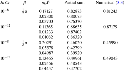
As shown in table 1, for  $\beta ={\textstyle \frac {1}{3}}{\rm \pi}$ and
 $Ja\,Cr=10^{-8}$, only
 $a_1\lambda = 0.20291$ significantly exceeds the corresponding value of
 $\delta = 0.05540$; including terms of higher order in the partial sum amounts to over-interpreting (6.1). Comparing the entries in columns
 $4$ and
 $5$ in table 1 verifies that truncating at
 $O(\lambda )$ gives the closest approximation to the numerical solution of (3.3). For the smaller value
 $Ja\,Cr=10^{-12}$, the same argument suggests that the next term
 $a_2\lambda ^2$ is significant, and should be included; comparing the appropriate entries in table 1 verifies that this gives a (slightly) closer approximation. Figure 6 is consistent with this conclusion.
According to the discussion in § 6.3, the error in (6.1) is smaller for  $\beta ={\textstyle \frac {1}{2}}{\rm \pi}$; it is then
 $O(\lambda \delta )$, i.e. about
 $0.02$ and
 $0.003$ for the two values of
 $Ja\,Cr$ used in table 1. This suggests that truncating at higher order should improve the approximation. For
 $Ja\,Cr=10^{-8}$, the smallest value of
 $a_k\lambda ^2$ occurs for
 $k=2$ and truncating the series there indeed improves the approximation slightly. But the same argument suggests truncating at
 $O(\lambda ^3)$ at
 $Ja\,Cr=10^{-12}$, there it worsens the approximation. This behaviour is consistent with the statement by Olver (Reference Olver1974, p. 519) that ‘an upper bound for the error term of an asymptotic expansion can not be safely inferred simply by inspection of the rate of numerical decrease of the terms in the series at the point of truncation’.
For representative values of  $Ja\,Cr$, the term
 $O(\lambda ^3)$ is chiefly useful for demonstrating that the series (9.1) is unlikely to be convergent. It was, however, useful when (9.1) was used to provide starting values for numerical solutions of (3.3) for the smallest values of
 $Ja\,Cr$ included in figure 9.
9.3. Effect on $\chi$ of evaporation from the contact region

Two limiting cases have been identified in this paper, according as  $F/(Ja\,Cr)^{1/3}$ or
 $F$ is held fixed in the limit as
 $Ja\,Cr\to 0$. Consistency of the scales corresponding to these limiting case requires
 $\chi$ to be decreased by evaporation from the contact region.
For, when  $F/(Ja\,Cr)^{1/3}$ is held fixed (Appendix E),
 $h/(Ja\,Cr)^{1/3}$ is a function of
 ${\theta }/(Ja\,Cr)^{1/3}$, and the slope
 ${\rm d} h/{\rm d}{\theta }= O([Ja\,Cr]^{1/6})$, i.e. logarithmically smaller than its value
 $O(\delta )$ given by (6.5). In a sequence of numerical calculations in which
 $F$ is reduced from a value
 $O(1)$, and the apparent contact circle retreats from the equator towards the bottom of the sphere,
 $h_0/(C\delta )$ must therefore vary continuously with
 $\beta$ from a value
 $O(1)$ (appropriate for fixed
 $F$) to the smaller value occurring when
 $F/(Ja\,Cr)^{1/3}$ is fixed. As
 $\beta$ is reduced,
 $|\tau |$ increases without bound, and the higher terms in the series expansion (7.6c) increase in magnitude. The decrease in slope can only result if the coefficients
 $a_k$ are positive for small
 $\beta$, as in figure 8. Because the coefficients are indeed then positive,
 $\chi /(C\delta )$ necessarily decreases with increasing
 $\lambda$, i.e. with increasing evaporation from the contact region.
9.4. Nusselt number
From equations (6.5 f) and (7.2c) of the asymptotic analysis
 \begin{equation} -\frac{C\delta}{\log\delta}\,Nu= F^{1/2}\,Q_\infty(\tau, \lambda), \end{equation}
 $C= 1.30588$ (equation (7.8)) and
 $Q_\infty (\tau,\lambda )$ is given by the series (8.1). The solution depends on only two parameters
 $Ja\,Cr$ and
 $F=\sin ^2\beta$: in (9.3),
 $\tau = 0.23577 +\log \tan ({\textstyle \frac {1}{2}}\beta )$ (7.10) and
 $\delta$ is defined in terms of
 $Ja\,Cr$ by (6.2). The solution depends on superheat
 $\Delta T$ through the Jakob number
 $Ja$.
The Nusselt number varies as  $F^{1/2}$ because the area of a spherical cap increases as
 $\sin ^2({\textstyle \frac {1}{2}}\beta )$, but heat is conducted over a distance of the order of
 $h_0\propto \tan ({\textstyle \frac {1}{2}}\beta )$. In particular, for
 $\lambda \to 0$,
 $Q_\infty (\tau, \lambda )\to 1$ and
 \begin{equation} \frac{Nu}{C\lambda\delta} =F^{1/2}. \end{equation}
Figure 11 shows  $Nu$ as a function of
 $Ja\,Cr$ for
 $p_0=2$, approximating the state of maximum force. Symbols show values obtained from the numerical solution of (3.3). Lines show the result obtained by truncating the series in (9.3) at various orders. For the entire range of values of
 $Ja\,Cr$ included in the figure, truncating the series at
 $O(\lambda ^2)$ gives the closest approximation.


10. Conclusion
This work contains the first treatment allowing computation of the Nusselt number for the title problem using only the Laplace relation and the thin-film equations for the vapour motion and heat transfer. The problem of computing the volume flow rate  $q$ of the vapour, pressure
 $p$ within the vapour and the shape of the entire interface is reduced to one of solving a system of coupled ordinary differential equations. Because it is shown that in the limit as
 $Ja\,Cr\to 0$ (fixed
 $F$), both the total evaporation and the entire pressure variation are determined within the region where the thin-film approximation holds, this new method does not require patching of the numerical solution for the thin-film equations to a numerical solution of the full equations describing the outer thick film. Though the calculations are given here for the case in which the motion of the vapour is driven solely by the gradient in capillary pressure, the method should apply equally when the gradient in pressure imposed by the underlying liquid is equally important, or dominant. The method gives the Nusselt number
 $Nu$ with a relative error vanishing as
 $Nu^{-1}$.
By contrast, in van Limbeek et al. (Reference van Limbeek, Sobac, Rednikov, Colinet and Snoeijer2019), the total evaporation is not calculated. Film thickness and  $p$ are determined by integrating the thin-film equations up to a patching point chosen so that the angle between the interface and the drop surface has attained a given value (van Limbeek et al. Reference van Limbeek, Sobac, Rednikov, Colinet and Snoeijer2019, pp. 1184–1186). Thereafter,
 $p$ is set to zero in the Laplace relation. With the method developed here, the equations are simply integrated until
 $h$ has become sufficiently large that
 $p$ and
 $q$ have ceased to change.
That evaporation from the contact region decreases the apparent contact angle for the bubble cap is explained by comparing the magnitudes of the interface slope according as  $F/(Ja\,Cr)^{1/3}$ or
 $F$ is fixed in the limit as
 $Ja\,Cr\to 0$. There is no doubt as to the existence of the effect: asymptotic analysis shows it, the numerical solutions confirm it and logical consistency (§ 9.3) requires it. Because the reduction in contact angle thins the film for the entire bubble cap, it has a large effect on the Nusselt number. For realistic values of the parameters,
 $Nu$ is more than double the value it would have in the absence of this effect (figure 6). For the inverse Leidenfrost phenomenon this effect must weaken as
 $Bo$ is increased and surface tension becomes negligible except within the contact region. Numerical solutions to evaluate the effect on the total evaporation rate for
 $Bo$ of the order of unity are in progress.
Acknowledgements
I am grateful to M. Shi (Xi'an Jiaotong University) for introducing me to the subject; to Clay Radke for pointing out the connection with drop settling; to U. Thiele (University of Münster) for explaining that it is the method of continuation, not termination; and to three reviewers for their thoughtful reading of my work.
Declaration of interests
The author reports no conflict of interest.
Appendix A. Equivalent forms of the Laplace relation
By balancing forces on the ring formed when line element  ${\rm d} s$ (figure 1) is rotated about the
 $z$ axis,
 \begin{equation} \frac{{\rm d}}{{\rm d} s}({\sigma}\sin \alpha) = \left\{p +Bo\,z \right\} {\sigma} \frac{{\rm d} {\sigma}}{{\rm d} s};\quad\frac{{\rm d} {\sigma}}{{\rm d} s}= \cos\alpha, \quad \frac{{\rm d} z}{{\rm d} s}=\sin\alpha, \end{equation}
from the geometry of figure 1.
 \begin{equation} \frac{{\rm d} \alpha}{{\rm d} s}+\frac{\sin\alpha}{{\sigma}} =p + Bo\,z. \end{equation}
The first term on the left-hand side represents the curvature of the meridional cross-section (figure 1); the second term represents the corresponding second principal curvature.
Let  $r_{\theta }={\rm d} r/{\rm d} {\theta }$. By expressing (A2) in spherical coordinates,
 \begin{equation} \frac{r^2- rr_{{\theta}{\theta}} +2r_{\theta}^2}{(r^2+r_{\theta}^2)^{3/2}} +\frac{1-(r_{\theta}/r)\cot{\theta}}{(r_{\theta}^2+r^2)^{1/2}} = (p + Bo\,z)\,\mbox{sgn}\left(\frac{{\rm d} {\theta}}{{\rm d} s}\right). \end{equation}
The signum function enters because  ${\theta }$ is not a monotonic function of arc length
 $s$ in general (Appendix C). Terms on the left-hand side of the equality correspond to the principal curvatures identified above. In particular, the identity
 ${{\rm d} \alpha }/{{\rm d} s}= (r^2- rr_{{\theta }{\theta }} +2r_{{\theta }}^2)/(r^2+r_{{\theta }}^2)^{3/2}$ is equivalent to that for curvature of a plane curve in polar coordinates.
Appendix B. Similarity solution for the vapour film
This solution of the boundary-layer equations includes convective transport of heat, but not that of momentum. Units for pressure, velocity, length and temperature are those introduced in § 2. As in the text,  $r=1$ on the surface of the sphere and
 $1+h$ on the liquid–vapour interface.
In spherical coordinates, the boundary-layer form of the continuity equation is
 \begin{equation} \frac{{\partial} }{{\partial} r}(v_r\sin{\theta}) + \frac{{\partial} }{{\partial}{\theta}}(v_{\theta}\sin{\theta})=0. \end{equation}
This is satisfied by introducing the Stokes stream function  $\psi$:
 \begin{equation} v_r\sin{\theta} ={-}\frac{{\partial} \psi}{{\partial} {\theta}},\quad v_{\theta}\sin {\theta}=\frac{{\partial} \psi}{{\partial} r}. \end{equation}
With  $\psi =0$ on the surface of the sphere, the total flow rate is given by
 \begin{equation} 2{\rm \pi} q =2{\rm \pi} \psi(1+h,{\theta}) =2{\rm \pi} \int_1^{1+h} v_{\theta}\sin{\theta}\,{\rm d} r. \end{equation}
The dimensional volume flow rate is given by  $2{\rm \pi} b{\kappa } Ja\, q({\theta })$; the heat flow into the liquid–vapour interface is given by
 $\mathscr {Q}^*= 2{\rm \pi} \, b k\Delta T\,q$ (conductivity of the vapour,
 $k$).
Let
 \begin{equation} \xi =(r-1)/{h({\theta})}, \quad \psi= q(\theta)\,f(\xi), \quad T=g(\xi). \end{equation}
By the definition of  $q({\theta })$,
 $f(1)=1$.
Also let
 \begin{equation} {\varGamma}= \left. -h\frac{{\partial} T}{{\partial} r}\right|_{1+h}. \end{equation}
As part of the solution,  ${\varGamma }$ is obtained as a function of
 $Ja$.
Equations (B2a,b) satisfy the boundary-layer forms of the energy balances (2.2c), (2.2g) and the lubrication form of (2.2b) if
 \begin{equation} \frac{h }{\sin{\theta}}\frac{{\rm d} q}{{\rm d} {\theta}}={\varGamma},\quad \frac{h^3\sin{\theta}}{ Ja\,Cr q} \frac{{\rm d} p}{{\rm d} {\theta}}={-}c= f'''(\xi) \end{equation}
(separation constant  $c$) and
 \begin{equation} 0= Ja\,{\varGamma} fg'+g'', \quad 0<\xi<1. \end{equation}
The boundary conditions are
 \begin{gather} f(0)=f'(0)= 0, \quad g(0)=1; \end{gather}
 \begin{gather} f''(1)=0=g(1), \quad f(1)=1. \end{gather}
In the reduced heat equation (B5a), the effect of convective heat transport is described by the quantity  ${\varGamma }(Ja)$.
The solution of (B5c) satisfying all boundary conditions on  $f(\xi )$ is
 \begin{equation} f={\textstyle \frac{3}{2}}\xi^2 -{\textstyle \frac{1}{2}}\xi^3,\quad c=3. \end{equation}
The solution of (B5d) satisfying (B6e) is
 \begin{equation} g(\xi)= {\varGamma}\,\int_\xi^1 \mbox{e}^{Ja\,{\varGamma}\varphi(\xi)}\,{\rm d}\xi, \quad \varphi(\xi)= \int_\xi^1 f(\tau)\,{\rm d} \tau. \end{equation}
The function  ${\varGamma }(Ja)$ is determined by imposing the remaining condition (B6c):
 \begin{equation} 1 ={\varGamma}\int_0^1 \mbox{e}^ {Ja\,{\varGamma}\, \varphi(\xi)}\,{\rm d} \xi. \end{equation}
By expanding (B9) about  $Ja=0$,
 ${\varGamma }= 1+Ja\, {\varGamma }'_0 +{\textstyle \frac {1}{2}} Ja^2\,{\varGamma }''_0 +\cdots,$ where
 \begin{equation} {\varGamma}'_0={-}\int_0^1\varphi(\xi)\,{\rm d}\xi,\quad {\varGamma}''_0= 4\left(\int_0^1\varphi(\xi)\,{\rm d}\xi\right)^2 - \int_0^1\varphi^2(\xi)\,{\rm d}\xi. \end{equation}
In particular, for the conditions (B6b,d),  $\varphi (\xi )= {\textstyle \frac {1}{8}}(\xi ^4-4\xi ^3+3).$ The corresponding flux into the liquid–vapour interface is
 \begin{equation} \left.
-h\frac{{\partial} T}{{\partial}
r}\right|_{1+h}= {\varGamma}= 1-{\frac{11}{40}}Ja +
{\frac{21\,677}{201\,600}} Ja^2+\cdots;
\end{equation}
that from the sphere into the vapour is
 \begin{equation} \left.
-h\frac{{\partial} T}{{\partial}
r}\right|_{r=1}=
{\varGamma}\,\mbox{e}^{Ja{\varGamma}\,\varphi(0)}
= 1+{\frac{1}{10}}Ja -
{\frac{179}{6300}}Ja^2+\cdots.
\end{equation}
Vapour flows from the interface towards the sphere, thereby decreasing the flux from vapour into the liquid, but increasing that from the sphere into the vapour. The difference is transported downstream. Equations (B9) and (B11) are shown as figure 2 in the text.
Appendix C. Extended system (3.3)
C.1. Proof of the geometric identities (3.3d) and (3.3e)
In figure 12,  $C$ denotes the centre of the sphere;
 $P$ and
 $Q$ represent arbitrary points on the interface with position vectors
 $CP={\boldsymbol r}$ and
 $CQ={\boldsymbol r}+{\Delta }{\boldsymbol r}$. The limit as
 ${\Delta }{\theta }\to 0$ is taken only at the end of the argument following (C2).
Geometry used to prove the identities (3.3d,e): position vectors  $CP$ and
 $CQ$ of two arbitrary points on the interface;
 ${\Delta } {\theta } =\angle PCQ$ is of arbitrary magnitude.

By applying the sine rule to  $\triangle CPQ$ without approximation,
 \begin{equation} \frac{|{\boldsymbol r}+{ \Delta} {\boldsymbol r}|}{\cos({\theta}-\alpha)} = \frac{|{\boldsymbol r}|}{\cos({\theta}- \alpha +{\Delta} {\theta})}= \frac{|{\Delta}{\boldsymbol r}|}{\sin{ \Delta} {\theta}} \end{equation}
( $\sin ({\textstyle \frac {1}{2}}{\rm \pi} +A)\equiv \cos A$). By using (C1b), (C1a) can be expressed equivalently as
 \begin{equation} \frac{|{\boldsymbol r}+{\Delta} {\boldsymbol r}|-|{\boldsymbol r}|}{{|\Delta} {\boldsymbol r}|} ={-}\frac{\cos({\theta}-\alpha+{\Delta {\theta}})-\cos({\theta}-\alpha)}{\sin{\Delta}{\theta}}. \end{equation}
By taking the limit as  ${\Delta }{\theta }\to 0$, identity (3.3e) follows from (C1b); and identity (3.3d) follows from (C2). (The relations
 $|CP|=r =1+h$ and
 $|{\Delta } {\boldsymbol r}|/{\Delta } s\to 1$ have been used. Identities (3.3d) and (3.3e) can be also obtained using the expressions
 $r^2 ={\sigma }^2+z^2$,
 $\tan {\theta }= -{\sigma }/z$,
 ${\rm d} {\sigma }/{\rm d} s= \cos \alpha$ and
 ${\rm d} z/{\rm d} s= \cos \alpha$ following from the geometry of figure 1.)
C.2. Example illustrating the method used to compute $Nu$

In § 3, it is argued that in the limit as  $Ja\,Cr\to 0$, the film has an inner-and-outer structure, and that the outer region then contributes a vanishingly small fraction of the value of
 $Nu$ obtained by solving (3.3) numerically. The following example is given to demonstrate that this argument is not invalidated by the presence of the contact singularity in the outer solution for
 $q$.
The outer limit is  $Ja\,Cr\to 0$ (fixed
 $h$); in this limit, the pressure
 $p=0$, as given by (3.6b). The corresponding solution of the Laplace relation is (Princen Reference Princen1969, p. 6)
 \begin{equation} \frac{{\sigma}}{c_1}=\cosh\left(\frac{z-c_2}{c_1}\right), \end{equation}
with constants of integration  $c_1$ and
 $c_2$. This equation describes the surface of revolution generated by rotating a catenary about the
 $z$ axis:
 $z$ is a double-valued function of
 ${\sigma }$, on the catenary, the branch point is at
 $z=c_2$; there
 ${\sigma }=c_1$ and the tangent in the
 $\{{\sigma },z\}$ plane is vertical. Only part of the surface of revolution is physically relevant.
In the outer limit, film thickness vanishes at the apparent contact circle; by setting  $h=0$ in (3.5), i.e.
 ${\sigma }=(1+h)\sin {\theta }$ and
 $z=-(1+h)\cos {\theta }$, the catenary touches the sphere at
 ${\sigma }=\sin \beta$ and
 $z=-\cos \beta$; because the apparent contact angle measured through the liquid is equal to
 ${\rm \pi}$,
 ${{\rm d} z}/{{\rm d} {\sigma }}=\tan \beta$ at the apparent contact line.
Imposing these conditions on (C3) provides two equations determining  $c_1$ and
 $c_2$:
 \begin{equation} \frac{1}{c_1}\sin\beta =\cosh \left(\frac{\cos\beta+c_2}{c_1}\right),\quad \cot\beta={-}\sinh\left(\frac{\cos\beta+c_2}{c_1}\right). \end{equation}
By eliminating  $c_2$ between (C4a) and (C4b), then noting that (C4b) can be written equivalently as
 $c_2+\cos \beta = c_1\log (\tan {\textstyle \frac {1}{2}}\beta )$,
 \begin{equation} c_1=\sin^2\beta,\quad c_2 = (\sin^2\beta)\,\log \tan({\textstyle\frac{1}{2}}\beta) -\cos\beta. \end{equation}
By comparing (C5a) with (5.4),  $c_1=F$. (Because
 ${\sigma }\ge c_1$, and the tangent to the catenary is vertical at the minimum value of
 ${\sigma }$, the vertical component of force exerted by surface tension on the interface is
 $2{\rm \pi} c_1$, whence
 $c_1=F$.)
Using this solution of the Laplace relation, the outer solution for  $q$ is obtained in explicit form. By eliminating
 ${\rm d} {\theta }/{\rm d} s$ between (3.3b) and (3.3e),
 \begin{equation} \frac{{\rm d} q}{{\rm d} s}=\frac{\sin{\theta}\,\cos({\theta}-\alpha)}{h(1+h)} =\sigma \frac{\cos({\theta}-\alpha)}{h(1+h)^2}, \end{equation}
where (3.5a) has been used to obtain (C6b). Further, by (A1b) and (A1c),
 \begin{equation} \cos({\theta}-\alpha) =\left({\sigma} \frac{{\rm d} z}{{\rm d} s} -\left. z\frac{{\rm d}{\sigma}}{{\rm d} s}\right)\right/ \left(1+h\right). \end{equation}
Thus,
 \begin{equation} \frac{{\rm d} q}{{\rm d} z} = \left({\sigma}-z\frac{{\rm d}{\sigma}}{{\rm d} z}\right)\frac{{\sigma}}{h(1+h)^3}, \end{equation}
where  $z$ has been introduced as the independent variable. Because
 $h=({\sigma }^2+z^2)^{1/2}-1$, the right-hand side of (C8) is a known function of
 $z$.
C.3. Solution of (C8) for $\beta ={\textstyle \frac {1}{2}}{\rm \pi}$

For this case, the apparent contact circle is at the equator of the sphere, and by (C5),  $c_1=1$ and
 $c_2=0$. Thus
 $(1+h)^2 =\cosh ^2 z+z^2$ and
 \begin{equation} \frac{{\rm d} q}{{\rm d} z} = \frac{\cosh^2 z -{\textstyle\tfrac{1}{2}} z\sinh 2z} {\left([\cosh^2 z+z^2]^{1/2}-1\right) \left[\cosh^2 z+z^2\right]^{3/2} }. \end{equation}
Let  $\omega$ be an arbitrary function of
 $Ja\,Cr$. Also let
 $c_3$ be an arbitrary constant independent of
 $Ja\,Cr$. Then, by integrating (C9) from
 $\infty$ to
 $z$,
 \begin{equation} q = \omega\, c_3 - \int_z^\infty \frac{\left(\cosh^2 v -{\textstyle\tfrac{1}{2}} v\sinh 2v\right)\, {\rm d} v}{\left([\cosh^2 v+v^2]^{1/2}-1\right)\,\left[\cosh^2 v+v^2\right]^{3/2}\,} \end{equation}
(dummy variable of integration  $v$). The constant of integration
 $\omega \,c_3$ is to be determined by matching to the solution for the thin film. The contribution of the outer region to the total evaporation is given by the integral term in (C10). This term is independent of
 $Ja\,Cr$; in this sense, it is
 $O(1)$, even though the integral diverges as
 $z\to 0$, as is shown next.
Matching requires the asymptotic expansion of (C10) as  $z\to 0$. It was obtained by splitting the interval of integration into subintervals:
 $z< v<\varepsilon$ and
 $\varepsilon < v<\infty$ (
 $\varepsilon \ll 1$, to be chosen). The contribution from the second interval was obtained numerically; that from the first, by termwise integration of the series
 \begin{equation} \frac{{\rm d} q}{{\rm d} z} = z^{{-}2}- \frac{8}{3} +\frac{244}{45}z^2+\cdots. \end{equation}
For  $0< z\ll 1$, therefore,
 \begin{equation} q = \omega c_3 -z^{{-}1} + c_4 +O(z), \end{equation}
where
 \begin{align} c_4 =\lim_{\varepsilon\to 0} \left\{\varepsilon^{{-}1} +\frac{8}{3}\varepsilon - \frac{244}{135} \varepsilon^3- \int_\varepsilon^ \infty \frac{\left(\cosh^2 v -{\textstyle\tfrac{1}{2}} v\sinh 2v\right)\, {\rm d} v} {\left([\cosh^2 v+v^2]^{1/2}-1\right)\,\left(\cosh^2 v+v^2\right)^{3/2}\,}\right\}. \end{align}
Using either  $\varepsilon =0.01$ or
 $0.001$ gives
 $c_4= 2.87120$.
At the outer edge of the contact region, the outer solution overlaps with that for the thin film. By introducing the inner variables defined by (6.5) for the thin film, the expression  $z=-(1+h)\cos {\theta }$ becomes
 $z= \hat {\theta }\,\delta +O(\delta ^2)$. With this substitution, and the corresponding substitution
 $q= \hat q/(\lambda \delta )$ given by (6.5 f), the inner limit (C12a) of the outer solution is found to be
 \begin{equation} \hat q_{\rm outer}\sim \lambda\delta\,\omega c_3 - \lambda \hat{\theta}^{{-}1} + \lambda\delta\,c_4. \end{equation}
The outer limit of the inner solution describing the film is obtained in two steps: by integrating (6.7d),  $\hat h\sim \hat {\theta }^2 +O(\hat {\theta })$, then substituting that expression into (6.7c) and integrating to show that
 \begin{equation} \hat q_{\rm inner} \sim c_5 -\lambda \hat {\theta}^{{-}1} +O(\hat{\theta}^{{-}2}). \end{equation}
The constant  $c_5$ is a property of the solution of problem (6.7). Consequently, it depends on
 $\lambda$ but is independent of
 $\delta$; in the limit as
 $\lambda \to 0$,
 $c_5$ approaches a non-zero constant.
Matching of the leading terms in (C13) and (C14) requires that
 \begin{equation} \lambda \delta\,\omega c_3= c_5,\quad \omega= (\lambda\delta)^{{-}1}, \quad c_5=c_3. \end{equation}
In (C13) and (C14), the terms in  $\hat {\theta }^{-1}$ are matched. The remaining term containing
 $c_4$ is
 $o(1)$. It is not matched because for
 $\beta ={\textstyle \frac {1}{2}}{\rm \pi}$, the error in the solution for the thin film is also
 $O(\lambda \delta )$, as noted in § 6.3. For
 $\beta ={\textstyle \frac {1}{2}}{\rm \pi}$, the numerical solution of (3.3) therefore determines
 $Nu$ with relative error vanishing as
 $\lambda \delta$, i.e. as
 $Nu^{-1}$. This is consistent with the discussion in § 3.
Appendix D. Derivation of certain coefficients in (7.19)
The derivative of a function of a single variable is denoted by a prime:  $H_0'= {\rm d} H_0/{\rm d} {\varTheta }$ and
 $a_1' ={\rm d} a_1/{\rm d} \tau$. A partial derivative of a function of two or more variables is denoted by a subscript:
 $H_{1\tau }= {\partial } H_1/ {\partial }\tau$.
D.1. First correction
Because  $H_{0\tau }=0$, equation (7.12a) requires
 $Q_{1\tau }$ to be independent of
 ${\varTheta }$. Imposing (7.12d) gives
 $Q_{1\tau }= a_1'+1$. The remaining members of (7.12) require that
 \begin{gather} {{\mathscr{D}} } H_{1\tau}= (a_1'+1)\,H_0, \quad -\infty<{\varTheta}<\infty ; \end{gather}
 \begin{gather} \left. \frac{{\rm d} H_{1\tau}}{{\rm d} {\varTheta}}\right|_{-\infty}=a_1',\quad \left. \frac{{\rm d}^2 H_{1\tau}}{{\rm d}{\varTheta}^2}\right|_\infty=0. \end{gather}
The operator  ${{\mathscr {D}} }$ is defined by (7.11). A solution of (D1) is
 \begin{equation} H_{1\tau} ={\textstyle\frac{1}{3}}H_0 -{\textstyle \frac{1}{6}}{\varTheta} H_0'({\varTheta}), \quad a_1'(\tau)={-}{\textstyle\frac{1}{6}}. \end{equation}
Because  $F= H'_0({\varTheta })$ satisfies the homogeneous problem
 ${{\mathscr {D}} } F=0$,
 $F'(-\infty )=0=F''(\infty )$, any multiple of
 $H_0'$ could be added to (D2) without changing
 $a'_1(\tau )$. Because
 $H_{1\tau }'(\infty )$ would change, it cannot be determined from (D2), but only by solving the complete problem (7.12).
D.2. Second correction
From (7.15),  $Q_{2\tau \tau }= a_2'' -\frac {5}{18}$ and
 \begin{gather} {{\mathscr{D}} }
[H_{2\tau\tau}]=\left(a_2'' -{\frac{11}{18}}\right) H_0
-{\frac{1}{2}}{\varTheta} H_0' +
{\frac{1}{3}}{\varTheta}^2 \frac{H_{0}'^2}{H_0},
\quad -\infty<{\varTheta}<\infty ;
\end{gather}
 \begin{gather} \left. \frac{{\rm d} H_{2\tau\tau}}{{\rm d} {\varTheta}}\right|_{-\infty}=a_2'',\quad \left. \frac{{\rm d}^2 H_{2\tau\tau}}{{\rm d}{\varTheta}^2}\right|_\infty=0. \end{gather}
A solution is
 \begin{equation} H_{2\tau\tau}={-}{\textstyle\frac{2}{9}}H_0 +{\textstyle\frac{1}{12}}{\varTheta} H_0'({\varTheta}) + {\textstyle\frac{1}{36}}\,{\varTheta}^2 H_0''({\varTheta}), \quad a_2''(\tau)={\textstyle\frac{5}{36}}. \end{equation}
D.3. Third correction
From (7.17),  $Q_{3\tau \tau \tau }= a_3'''+\frac {5}{12}$ and
 \begin{gather} {{\mathscr{D}} }
[H_{3\tau\tau\tau}]=
\left(a_3'''+{\frac{17}{18}}\right)\,H_0
+{\frac{3}{2}}{\varTheta} H_0'
-{\frac{4}{3}}{\varTheta}^2\frac{H_0'^2}{H_0}
+{\frac{1}{8}}{\varTheta}^2H_0''
+{\frac{1}{18}}{\varTheta}^3\frac{H_0'}{H_0}
\left\{5\frac{H_0'^2}{H_0}-3 H_0''\right\}
; \end{gather}
 \begin{gather} \left. \frac{{\rm d} H_{3\tau\tau}}{{\rm d} {\varTheta}}\right|_{-\infty}=a_3''',\quad \left. \frac{{\rm d}^2 H_{3\tau\tau}}{{\rm d}{\varTheta}^2}\right|_\infty=0. \end{gather}
A solution is
 \begin{align} H_{3\tau\tau\tau}= {\textstyle\frac{10}{27}}H_0 -{\textstyle\frac{25}{216}}{\varTheta} H_0'({\varTheta}) -{\textstyle\frac{5}{72}}{\varTheta}^2H_0''({\varTheta}) -{\textstyle\frac{1}{216}}{\varTheta}^3 H_0'''({\varTheta}), \quad a_3'''(\tau)={-}{\textstyle\frac{55}{216}}. \end{align}
Appendix E. Boundary-value problem cited in the discussion of figure 3
Solid curves in figure 3 were obtained by solving the simplified system obtained from (3.3) by assuming  $p$,
 $q$ and
 $h$ to vary with respect to
 ${\theta }$ on a single scale
 ${\theta }_s\ll 1$.
Let
 \begin{equation} p=p_s p', \quad q=q_s q', \quad h=h_s h', \quad {\theta}= {\theta}_s {\theta}', \quad {\sigma}={\theta}_s{\sigma}', \quad r= 1+h_s r', \end{equation}
so that on the sphere  $r'=0$ (and a prime does not denote a derivative). By balancing terms in (3.3) and in (A3), the scales are found to be
 $h_s=(Ja\,Cr)^{1/3}$,
 ${\theta }_s=(Ja\,Cr)^{1/6}$ and
 $p_s=1=q_s$. Hence,
 \begin{gather} p= p', \quad q= q', \quad h=(Ja\,Cr)^{1/3} h', \quad {\theta}=(Ja\,Cr)^{1/6} {\theta}', \end{gather}
 \begin{gather} z-(c-1) =(Ja\,Cr)^{1/3}({\textstyle\frac{1}{2}}{\theta}'^2 -r'), \quad {\sigma}' ={\theta}'. \end{gather}
Variables with primes describe a small region near  ${\theta }=0$. Within it, the radius
 ${\sigma }$ in cylindrical coordinates is equivalent to the polar angle
 ${\theta }$ in spherical coordinates, and the sphere
 $r'=0$ is approximated by a paraboloid. The same approximation underlies Taylor's solution for the squeeze flow driven by the mutual approach of two rigid spheres (Horn et al. Reference Horn, Vinogradova, Mackay and Phan-Thien2000, note 38).
By substituting (E2) into (3.3), then taking the limit as  $Ja\,Cr\to 0$ (fixed
 ${\theta }'$),
 \begin{equation} - h'^3{\theta}' \frac{{\rm d} p'}{{\rm d} {\theta}'}= 3 q',\quad \frac{h'}{{\theta}'}\frac{{\rm d} q'}{{\rm d} {\theta}'}=1, \quad \frac{1}{{\theta}'}\frac{{\rm d}}{{\rm d} {\theta}'}\left[ {\theta}' \frac{{\rm d} h'}{{\rm d} {\theta}'}\right]=2- p', \end{equation}
for  $0< {\theta }'<\infty$. The boundary conditions are
 \begin{equation} \mbox{ at } {\theta}'=0, \quad p'= p'_0, \quad h'=h'_0; \mbox{ as }{\theta}'\to \infty,\> p'\to 0. \end{equation}
The equilibrium condition (3.6) requires that
 \begin{equation} \frac{F}{(Ja\,Cr)^{1/3}}= \int_0^\infty p'\,{\theta}'{\rm d} {\theta}'. \end{equation}
The method of solution is identical to that used for (3.3): with  $p'_0$ assigned,
 $h'_0$ is chosen to satisfy (E3 f), and the corresponding value of
 $F/(Ja\,Cr)^{1/3}$ is obtained from (E3g).
To derive (E3),  $p$,
 $q$ and
 $h$ were assumed to vary with respect to
 ${\theta }$ on a single scale. The assumption is self-consistent provided
 $F/(Ja\,Cr)^{1/3}$ is fixed in the limit as
 $Ja\,Cr\to 0$. With the limit thus defined, (E3) contains no large parameter and all dependent variables are
 $O(1)$. Viewed at the scale of the sphere, the liquid–vapour interface and the sphere appear to touch at a single point
 ${\theta }=0$: there is an apparent contact point rather than an apparent contact circle. Now, according to figure 3(a), as
 $F/(Ja\,Cr)^{1/3}$ is increased,
 $p'$ remains of the order of unity. Consequently, the force balance (E3g) can only be satisfied if
 $p'$ acts over an increasing area. A separation of scales develops as a result, and the apparent contact point becomes the apparent contact circle of a bubble cap (Brandão & Schnitzer Reference Brandão and Schnitzer2022, p. 1130).
Once this bubble cap is present in the solution of (E3),  $p_0'>2$ because from (E3c),
 \begin{equation} \left. \frac{{\rm d}^2 h'}{{\rm d} {\theta}'^2}\right|_0 = {\frac{1}{2}}(2-p_0'), \end{equation}
and this must be negative in order for the two paraboloids to intersect. Numerical solutions of (E3) show that as  $F/(Ja\,Cr)^{1/3}\to \infty$,
 $p_0'\to 2$ from above. In figure 3(a), the asymptote
 $p_0'=2$ is shown by the broken line. The corresponding response curves are single-valued. (The argument leading to (E4) does not hold when
 $F=O(1)$ because both principal curvatures are then of comparable size, as can be seen from (5.1) and (5.2).)
For the small values of  $F$ described by this limit, the numerical method described in Appendix C ceases to be useful because the contribution of the thick film is no longer small. Specifically, in the solution of (E3), there is no separation of scales in general. As a result,
 $q'$ grows as
 $\log {\theta }'$ as
 ${\theta }'\to \infty$, rather than approaching a limit as it does for the solution of (6.7). The Nusselt number is consequently only logarithmically large in
 $Ja\,Cr$ because the singularity in the solution for the outer region where film thickness is comparable with the sphere is logarithmic for small
 $F$ rather than being algebraic, as it is for fixed
 $F=O(1)$.


 Open access

