I. INTRODUCTION
The Nitinol 60 shape memory alloy (60 wt% Ni, 40 wt% Ti), which is first developed by US Navy in the early 1960s, has been a primary candidate material for aircraft due to its good mechanical and chemical properties, Reference Zeng and Dong1–Reference Adharapurapu and Vecchio3 for example, hardness up to 62RC, nonmagnetic, excellent corrosion resistance, high-yield strength, and lower density. Thermomechanical processing is found to be an important processing step during manufacturing of this alloy. Nevertheless, Nitinol 60 alloy exhibits poor workability attributed to the presence of considerable amount of intermetallic phases. Reference Dehghani and Khamei4–Reference Khamei and Dehghani6 As a matter of course, how to find a way to predict and analyze the deformation behavior under different thermomechanical conditions is the primary concern in this regard.
The development of numerical simulation techniques has opened invaluable windows to the finite element method (FEM) to successfully and widely be applied for analyzing and optimizing the materials forming processes. Reference Shamsolhodaei, Zarei-Hanzaki, Ghambari and Moemeni7,Reference Fatemi-Varzaneh, Zarei-Hanzaki and Haghshenash8 Constitutive equation is considered as an input of the FEM code for simulating the response of materials under specified loading condition, Reference Shamsolhodaei, Zarei-Hanzaki, Ghambari and Moemeni7,Reference Samantaray, Mandal and Bhaduri9 which will have a significant effect on the accuracy of the numerical simulation.
Over the past few years, various analytical, phenomenological, and empirical models have been constructed to predict constitutive behavior. A comprehensive review on constitutive analysis in hot working of austenitic stainless steel, carbon and alloy steels, ferritic steel, and Al alloy could be found in Ref. Reference McQueen and Ryan10. An internal state variable-based self-consistent constitutive model was proposed for Ti–6Al–4V alloy. Reference Fan and Yang11 Among the phenomenological models, Arrhenius type equations and their modified forms were extensively applied to describe the hot deformation behavior of materials. A strain-dependent parameter into the sine hyperbolic constitutive equation was introduced by Sloof et al. Reference Slooff, Zhou, Duszczyk and Katgerman12 The constitutive equations for pure titanium at temperature ranges of 350–500 °C Reference Rezaei Ashtiani, Parsa and Bisadi13 and 400–700 °C Reference Zeng, Jonsson and Zhang14 were proposed by using Arrhenius type equation, and the influence of strain was incorporated in the constitutive equation by considering the effects of strain on material constants (i.e., A, β, and activation energy Q). A modified sine hyperbolic constitutive equation was adopted by incorporating strain and strain rate to predict the elevated temperature flow behavior in D9 alloy and TC4-DT alloy. Reference Mandal, Rakesh, Sivaprasad, Venugopal and Kasiviswanathan15,Reference Peng, Guo, Shi, Qin and Zhao16 On the other hand, Guan et al. Reference Guan, Ren, Zhao, Ma and Wang17 proposed an empirical relation for superplastic behavior of Al–Zn–Mg–Zr alloy. Quan et al. Reference Quan, Liu, Zhou and Chen18 established the constitutive model of 7075 aluminum alloy containing a softening rate item by the multiple-linear regression method.
However, the accuracy is usually not high enough in some case by using both phenomenological and empirical models because of their lack of physical background. Recently, artificial neural network (ANN) has been a powerful alternative approach in the prediction of constitutive relationships, especially for complex and nonlinear systems. Some valuable studies have been conducted regarding the applications of ANN, which has been developed and successfully used to study the flow behavior in a variety of alloys. A comparative study was made on the capability of the Arrhenius type, multiple-linear, and ANN models for Ti600 alloy. Reference Zhao, Ding, Zhao, Huang, Wei and Jiang19 The result indicated that the ANN model was much more efficient and had higher accuracy than the other two models. Han et al. Reference Han, Qiao, Sun and Zou20 developed an optimized back-propagation (BP) neural network model to describe the compressive deformation behavior for the as-cast 904L stainless steel. The result showed that the optimized ANN model with three hidden layers had excellent predictability of flow stress. In addition, such ANN models had been already adopted to predict the high-temperature flow behavior of AZ81 magnesium alloy, Reference Sabokpa, Zarei-Hanzaki, Abedi and Haghdadi21 NiTi shape memory alloy, Reference Fatemi-Varzaneh, Zarei-Hanzaki and Haghshenash8 and Zr–2.5Nb–0.5Cu alloy. Reference Kapoora, Palb and Chakravarttya22
In this review, a comparative study has been made on the performance of phenomenological, empirical, and ANN models in predicting the hot deformation behavior of the as-forged Nitinol 60 alloy. The purpose of this investigation is to find out a suitable approach to model the flow behavior of Nitinol 60 alloy. Toward this end, isothermal hot compression tests were conducted in a wide range of strain rates and temperatures. The experimental stress–strain data were then used to drive the required material constants. Finally, the validity of developed constitutive models was examined and compared with each other for the entire experimental range.
II. EXPERIMENTAL PROCEDURES
The as-received billet was machined into cylindrical compression specimens with dimensions of 8 mm in diameter and 12 mm in height. Isothermal constant strain rate compression tests were conducted on a Gleeble-3500 hot simulator at 50 °C intervals in the temperature range of 650–850 °C, with the strain rate range of 0.01, 0.1, and 1 s−1. The specimens were heated at a rate of 10 °C/s up to 900 °C, soaked for 15 min, and then cooled at a rate of 10 °C/s down to the deformation temperature; they were then held for 3 min to ensure uniform temperature. All the specimens were compressed to a reduction in size of 50%, which is equivalent to a true strain of 0.7. They were immediately water quenched after compression testing. The deformed specimens were sectioned into two parts along the compression direction, and the cut surfaces were polished and etched in a solution of HF + HNO3 + H2O. The microstructures were then observed using optical microscope and scanning electron microscope.
III. RESULTS AND DISCUSSION
A. The initial microstructure
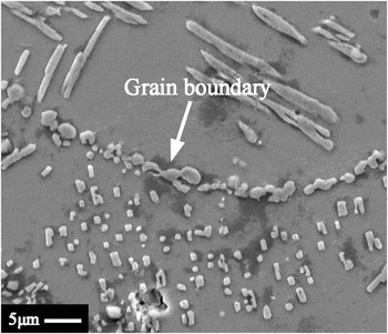
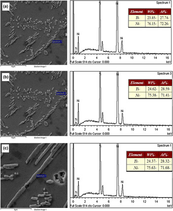
The as-received Nitinol 60 alloy billet used in this study, whose microstructure is presented in Fig. 1, was prepared by forging. From the Ni–Ti phase diagram, Reference Otsuka and Ren23 it can be shown that the Ni3Ti phase can precipitate out, during cooling after casting, and/or from the two-phase region after hot working. From Fig. 1, it can be seen that the precipitates are located both at the grain boundaries and within the matrix. In the first case, a particle morphology is exhibited, whereas the latter appears either as a strip or particle. Energy dispersive x-ray spectroscopy (EDX) analyses of the precipitates indicate the composition of intermetallic phase as Ni3Ti (shown in Fig. 2).
Microstructure of the as-received Nitinol 60 alloy.

EDX analyses of precipitates: (a) particle precipitate on the grain boundaries, (b) particle precipitate within matrix, and (c) strip precipitate within matrix.

B. The characteristics of flow stress
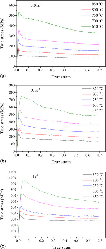
Typical stress–strain curves at different temperatures and strain rates are shown in Fig. 3. From Fig. 3, in the initial stage, all these curves exhibit similar features. The dominant work hardening, obviously, leads to the rapid increase of flow stress, until a peak value is reached. Beyond this, dynamic softening becomes dominant. For temperatures of 600 and 700 °C, the flow stress decreases monotonically. While, for temperatures of 750–850 °C, there is a plateau in the stress–strain curve at which dynamic balance between work hardening and dynamic softening is established. It should be noted that the flow stresses are strongly dependent on the deformation temperature and strain rate. Increasing the deformation temperature or decreasing the strain rate can result in the decrease of flow stress. This is because a low-strain rate and a high deformation temperature may accelerate the dislocations escape from the pinning of Ni3Ti. Reference Khamei and Dehghani6
The stress–strain curves at different strain rates and temperatures: (a) 0.01 s−1, (b) 0.1 s−1, and (c) 1 s−1.

C. Arrhenius type constitutive model
The correlation between flow stress, strain rate, and deformation temperature during hot deformation at a given strain can be expressed by the Arrhenius-type equation as follows Reference Sellars and McTegart24 :
 $$\dot \varepsilon = Af\left( \sigma \right)\exp \left( { - {Q \mathord{\left/ {\vphantom {Q {RT}}} \right. \kern-\nulldelimiterspace} {RT}}} \right)\quad ,$$
where
 $$f\left( \sigma \right) = \left\{ \matrix{ {\alpha ^{{n_1}}}{\kern 1pt} {\kern 1pt} {\kern 1pt} {\kern 1pt} {\kern 1pt} {\kern 1pt} {\kern 1pt} {\kern 1pt} {\kern 1pt} {\kern 1pt} {\kern 1pt} {\kern 1pt} {\kern 1pt} {\kern 1pt} {\kern 1pt} {\kern 1pt} {\kern 1pt} {\kern 1pt} {\kern 1pt} {\kern 1pt} {\kern 1pt} {\kern 1pt} {\kern 1pt} {\kern 1pt} {\kern 1pt} {\kern 1pt} {\kern 1pt} {\kern 1pt} {\kern 1pt} {\kern 1pt} {\kern 1pt} {\kern 1pt} {\kern 1pt} {\kern 1pt} {\kern 1pt} {\kern 1pt} {\kern 1pt} {\kern 1pt} {\kern 1pt} {\kern 1pt} {\kern 1pt} {\kern 1pt} {\kern 1pt} {\kern 1pt} {\kern 1pt} {\kern 1pt} {\kern 1pt} {\kern 1pt} {\kern 1pt} {\kern 1pt} {\kern 1pt} {\kern 1pt} {\kern 1pt} {\kern 1pt} {\kern 1pt} {\kern 1pt} {\kern 1pt} {\kern 1pt} {\kern 1pt} {\kern 1pt} {\kern 1pt} {\kern 1pt} {\kern 1pt} {\kern 1pt} {\kern 1pt} \alpha \sigma \;\lt\; 0.8 \hfill \cr \exp \left( {\beta \sigma } \right){\kern 1pt} {\kern 1pt} {\kern 1pt} {\kern 1pt} {\kern 1pt} {\kern 1pt} {\kern 1pt} {\kern 1pt} {\kern 1pt} {\kern 1pt} {\kern 1pt} {\kern 1pt} {\kern 1pt} {\kern 1pt} {\kern 1pt} {\kern 1pt} {\kern 1pt} {\kern 1pt} {\kern 1pt} {\kern 1pt} {\kern 1pt} {\kern 1pt} {\kern 1pt} {\kern 1pt} {\kern 1pt} {\kern 1pt} {\kern 1pt} {\kern 1pt} {\kern 1pt} {\kern 1pt} {\kern 1pt} {\kern 1pt} {\kern 1pt} {\kern 1pt} {\kern 1pt} {\kern 1pt} {\kern 1pt} {\kern 1pt} \,\,\,\alpha \sigma > 1.2 \hfill \cr {\left[ {\sinh \left( {\alpha \sigma } \right)} \right]^n}\quad {\kern 1pt} {\kern 1pt} {\kern 1pt} {\kern 1pt} {\kern 1pt} {\kern 1pt} \,\,\,\,\,\,\,\,\,{\rm{for}}\;{\rm{all}}\;\sigma \hfill \cr} \right.\quad .$$
In these equations,
 $\dot \varepsilon$
is the strain rate (s−1), σ is the flow stress (MPa) for a given strain, T is the absolute temperature (K), R is the universal gas constant (8.3144 J mol−1 K−1), Q is the deformation activation energy (J mol−1), and A, n
1, n, β, and α (α = β/n
1) are material constants. Generally, power law description is preferred for relatively lower stresses (i.e., ασ < 0.8) and the exponential law description is suitable for higher stresses (ασ < 1.2). This is while the hyperbolic sine law can be applied for a wide range of stress levels. Therefore, the hyperbolic sine law is generally preferred compared to the exponential and power law description. However, the first two equations are commonly used to extract n
1 and β, and then to calculate α.
The true stress–strain data obtained from the compression tests at various processing conditions, such as deformation temperature and strain rate, were used to evaluate the material constants of the constitutive equations. In this study, the strain of 0.2 was taken as an example to determine the material constants. Substituting the power law and exponential law description of f(σ) into Eq. (1), the following equations are derived:
 $$\dot \varepsilon = {A_1}{\sigma ^{{n_1}}}\exp \left( {{{ - Q} \mathord{\left/ {\vphantom {{ - Q} {RT}}} \right. \kern-\nulldelimiterspace} {RT}}} \right)\quad ,$$
 $$\dot \varepsilon = {A_2}\exp \left( {\beta \sigma } \right)\exp \left( {{{ - Q} \mathord{\left/ {\vphantom {{ - Q} {RT}}} \right. \kern-\nulldelimiterspace} {RT}}} \right)\quad ,$$
where A 1 and A 2 are the material constants. Taking the logarithm on both sides of Eqs. (3) and (4), respectively, we obtain:
 $$\ln \dot \varepsilon = \ln {A_1} + {n_1}\ln \sigma - {Q \mathord{\left/ {\vphantom {Q {RT}}} \right. \kern-\nulldelimiterspace} {RT}}\quad ,$$
 $$\ln \dot \varepsilon = \ln {A_2} + \beta \sigma - {Q \mathord{\left/ {\vphantom {Q {RT}}} \right. \kern-\nulldelimiterspace} {RT}}\quad .$$
Eventually, the values of n
1 and β are obtained from the mean slope values of
 $\ln \dot \varepsilon - \ln \sigma$
plot and
 $\ln \dot \varepsilon - \sigma$
plot [Figs. 4(a) and 4(b)]. They are found to be 5.8509 and 0.0191 MPa−1. Then the value of
 $\alpha = {\beta \mathord{\left/ {\vphantom {\beta {n_1 }}} \right. \kern-\nulldelimiterspace} {n_1 }} = 0.003261$
MPa−1 can be gained.
Evaluating the value of (a) n
1 by plotting
 $\ln \dot \varepsilon - \ln \sigma$
and (b) β by plotting
 $\ln \dot \varepsilon - \sigma$
.

For all range of stress level (including low- and high-stress levels), Eq. (2) can be represented as the hyperbolic sine law:
 $$\dot \varepsilon = A{\left[ {\sinh \left( {\alpha \sigma } \right)} \right]^n}\exp \left( {{{ - Q} \mathord{\left/ {\vphantom {{ - Q} {RT}}} \right. \kern-\nulldelimiterspace} {RT}}} \right)\quad .$$
Taking logarithm on both sides of Eq. (7), Eq. (8) is obtained:
 $$\ln \dot \varepsilon = \ln A + n\;\ln \left[ {\sinh \left( {\alpha \sigma } \right)} \right] - {Q \mathord{\left/ {\vphantom {Q {RT}}} \right. \kern-\nulldelimiterspace} {RT}}\quad .$$
The average of n value is found to be 4.1425 by the slope of
 $\ln \dot \varepsilon - \ln \left[ {\sinh \left( {\alpha \sigma } \right)} \right]$
[Fig. 5(a)]. ln A is also found from the interception of
 $\ln \dot \varepsilon - \ln \left[ {\sinh \left( {\alpha \sigma } \right)} \right]$
. For a particular strain rate, differentiating Eq. (8), we get:
 $$Q = Rn{\left[ {{{\partial \ln \left[ {\sinh \left( {\alpha \sigma } \right)} \right]} \over {\partial \left( {{1 \mathord{\left/ {\vphantom {1 T}} \right. \kern-\nulldelimiterspace} T}} \right)}}} \right]_{\dot \varepsilon }}\quad .$$
Evaluating the value of (a) n by plotting
 $\ln \dot \varepsilon - \ln \left[ {\sinh \left( {\alpha \sigma } \right)} \right]$
and (b) Q by plotting
 $\ln \left[ {\sinh \left( {\alpha \sigma } \right)} \right]$
−1/T.

Thus, the value of Q can be derived from the average slopes of plotting
 ${\kern 1pt} \ln \left[ {\sinh \left( {\alpha \sigma } \right)} \right] - {1 \mathord{\left/ {\vphantom {1 T}} \right. \kern-\nulldelimiterspace} T}$
under different strain rates, as shown in Fig. 5(b). The extracted activation energy is in the range of 264.43–319.50 kJ/mol for different strain values in the temperature range of 650–850 °C, which falls well between Q values reported for NiTi alloy in the literature.
Reference Shamsolhodaei, Zarei-Hanzaki, Ghambari and Moemeni7,Reference Khamei and Dehghani25
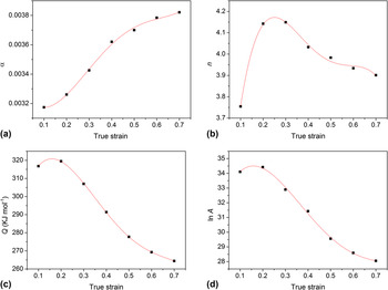
The values of α, n, Q, and lnA in Eq. (8) from experiments under different strains, as shown in Fig. 6, are further used to fit the fourth polynomial functions of strain (ε):
 $$\eqalignb{ & \alpha = {B_0} + {B_1}\varepsilon + {B_2}{\varepsilon ^2} + {B_3}{\varepsilon ^3} + {B_4}{\varepsilon ^4} \cr & n = {C_0} + {C_1}\varepsilon + {C_2}{\varepsilon ^2} + {C_3}{\varepsilon ^3} + {C_4}{\varepsilon ^4} \cr & \!Q = {D_0} + {D_1}\varepsilon + {D_2}{\varepsilon ^2} + {D_3}{\varepsilon ^3} + {D_4}{\varepsilon ^4} \cr & \!\!\!\!\!\!\!\ln A = {E_0} + {E_1}\varepsilon + {E_2}{\varepsilon ^2} + {E_3}{\varepsilon ^3} + {E_4}{\varepsilon ^4}\quad , \cr}$$
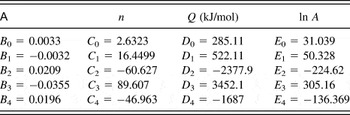
where the coefficients B i , C i , D i , and E i (i = 0, 1, 2, 3, 4) are summarized in Table I. Based on Eq. (8) and Table I, the deformation behavior of the as-forged Nitinol 60 alloy can be modeled and flow stress under the whole hot working conditions can be calculated.
Variations of (a) α, (b) n, (c) Q, and (d) lnA with true strain.

Coefficients of the polynomial for α, n, Q, and ln A.

D. Empirical model
For accurately modeling the constitutive relationship, the combined effects of strain, strain rate, and temperature on the flow stress are considered. Then, the multiple-linear constitutive model is defined as follows:
 $$\ln \sigma = {b_0} + {b_1}\varepsilon + {b_2}{1 \over T} + {b_3}\dot \varepsilon + {b_4}{\dot \varepsilon ^2} + {b_5}{{{{\dot \varepsilon }^2}} \over T}\quad ,$$
where b
0, b
1, b
2, b
3, b
4, and b
5 are constants. Let lnσ, ε, 1/T,
 $\dot \varepsilon$
,
 ${\dot \varepsilon ^2}$
, and
 ${{\dot \varepsilon ^2 } \mathord{\left/ {\vphantom {{\dot \varepsilon ^2 } T}} \right. \kern-\nulldelimiterspace} T}$
be y, x
1, x
2, x
3, x
4, and x
5, respectively, then Eq. (12) can be derived:
 $$y = {b_0} + {b_1}{x_1} + {b_2}{x_2} + {b_3}{x_3} + {b_4}{x_4} + {b_5}{x_5}\quad .$$
Given data set (y 1, x 11, x 21, x 31, x 41, x 51), (y 2, x 12, x 22, x 32, x 42, x 52), …, (y n , x 1n , x 2n , x 3n , x 4n , x 5n ) (n ≥ 5) under different strains, strain rates, and temperatures, the coefficients of b 0–b 5 in Eq. (12) could be regressed by the stepwise multiple-linear regression method. The calculated b 0–b 5 values are presented in Table II.
Regression coefficients in empirical constitutive model.

E. ANN model
ANN is an intelligent information treatment system with the characteristics of adaptive learning and treating complex and nonlinear relationships. It is essentially a ‘‘black box” operation linking input to output data using a particular set of nonlinear basis functions. With the development of technology of artificial intelligence, the ANN has become a powerful tool in the simulation and control of various processes.
A typical ANN architecture consists of an input layer, an output layer, and a hidden layer, which are connected by the processing units called neurons. Each neuron works as an independent processing element and has an associated transfer function. This transfer function describes how the weighted sum of its inputs is converted to the results into an output value. Among various kinds of ANN approaches, the feed-forward BP algorithm is adopted to model the flow behavior of the as-forged Nitinol 60 alloy. In the feed-forward BP network, the final calculated outputs are compared with the experimentally obtained outputs, and the errors are calculated. These errors are then propagated backwards and used for adjusting the weights of each of the neurons. The process of using the experimental outputs to minimize the mean squared error iteratively is called as training the network. The weights of the trained network are stored and can be used later for predicting outputs given a different set of inputs.
In the present work, the inputs are temperature, strain rate, and strain, while the output is stress. The ANN scheme necessitates that the range of both input data and output data should be within 0–1. Consequently, the data must be unified before inputting them into the network. The following equation is widely used for unification Reference Zhao, Ding, Zhao, Huang, Wei and Jiang19,Reference Sabokpa, Zarei-Hanzaki, Abedi and Haghdadi21 :
 $$X\prime = 0.1 + 0.8 \times \left( {{{X - {X_{\min }}} \over {{X_{\max }} - {X_{\min }}}}} \right)\quad ,$$
where X is the original data; X′ is the unified data corresponding to X; X
min and X
max are the minimum and maximum value of X, respectively. Since
 $\dot \varepsilon$
is changed sharply and the minimum
 $\dot \varepsilon$
value after unification is too small to be learned by the ANN model, the
 $\ln \dot \varepsilon$
will be used as the input instead of
 $\dot \varepsilon$
.
A total of 210 data sets were selected from the true stress–strain curves (with interval of 0.05 between the true strain of 0.05 and 0.7). From these data sets, 168 random data sets (80%) were used to train the ANN model, while the remaining 42 data (20%) were subsequently applied to test the performance of the ANN model.
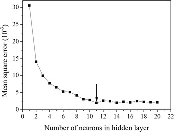
The next step in modeling using ANN is deciding the ANN architecture, which requires choosing appropriate number of hidden units. To decide the appropriate number of hidden layers, the trial-and-error procedure was carried out. Figure 7 shows the influence of number of neurons in hidden layer on the network performance. The values of mean square error were used to check the ability of a particular architecture. It is found that a network with one hidden layer consisting of 11 hidden neurons produces the best performance.
Influence of hidden-layer neurons on the network performance.

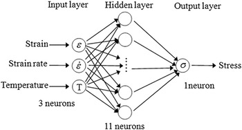
Hence, the developed ANN architecture (shown in Fig. 8), consisted of three input neurons (corresponding to temperature, strain, and strain rate), one intermediate hidden layer with 11 neurons and one output neurons (flow stress), was used to model the flow behavior of the as-forged Nitinol 60 alloy. The hidden layer uses a hyperbolic tangent sigmoid (tansig) transfer function, while the output layer uses a linear (purelin) transfer function to map the output parameters.
The ANN architecture (3-11-1).

F. Verification of constitutive models
The predictability of the constitutive equations (Arrhenius type, multiple-linear, and ANN models) is quantified using standard statistical parameters such as correlation coefficient (R) and average absolute relative error (AARE). These are expressed as:
 $$R = {{{\mathop\sum\limits_{i = 1}^N} \left( {{E_i} - \bar E} \right)\left( {{P_i} - \bar P} \right)} \over {\sqrt {{\mathop\sum\limits_{i = 1}^N\!{{\left( {{E_i} - \bar E} \right)}^2}{{\left( {{P_i} - \bar P} \right)}^2}} } }}\quad ,$$
 $${\rm{ARRE}}\left( \% \right) = {{1 \over N}\mathop\sum\limits_{i = 1}^N} \left| {{{{E_i} - {P_i}} \over {{E_i}}}} \right| \times 100\quad ,$$
where
 ${E_i}$
is the experimental data and
 ${P_i}$
is the predicted value obtained from the constitutive equations.
 $\bar E$
and
 $\bar P$
are the average values of E and P, respectively. N is the number of data, which were utilized in the investigation. R is a commonly used statistical parameter and provides information about the strength of linear relationship between the observed and calculated values. R is most often seen as a number between 0 and 1, which near 1 indicates that a regression line fits the data well, while it close to 0 indicates that a regression line does not fit the data very well. The higher value of R, however, may not always indicate better performance of an equation/model due to the tendency of the equation/model to be biased toward higher or lower values. Therefore, the AARE is also computed through a term-by-term comparison of the relative error thereby being an unbiased statistical parameter to measure the predictability of a model.
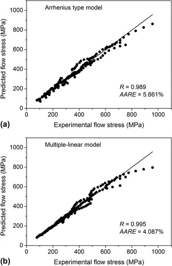
Figure 9 shows the diagrams by which the experimental values and predicted values are acquired from the Arrhenius type model and the multiple-linear model. As seen, the most of data points are laid close to the line inclined at 45°. The correlation coefficient and AARE for the Arrhenius type model are 0.989 and 5.661%, respectively, whereas those for the multiple-linear model are 0.995 and 4.087%, respectively. Thus, compared with the Arrhenius type model, the correlation of the multiple-linear model between predicted and experimental data is better.
The correlation between the experimental and predicted flow stress by (a) Arrhenius type model and by (b) multiple-linear model.

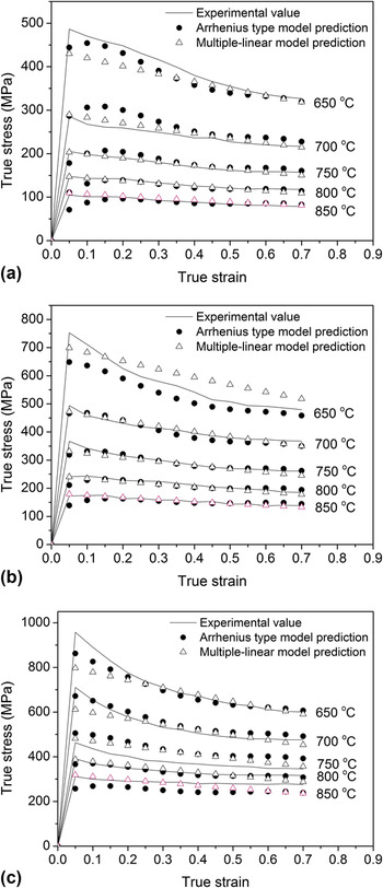
Figure 10 presents the comparative plots for experimental and predicted flow stress values. It can be seen that there is a remarkable deviation of predicted values from experimental values under some conditions (i.e., 650 °C, 0.1 s−1 and 850 °C, 1 s−1), indicating that both the Arrhenius-type and multiple-linear models cannot accurately track the flow behavior of the as-forged Nitinol 60 alloy.
Comparison between experimental and predicted flow stress at various strain rates of (a) 0.01 s−1, (b) 0.1 s−1, and (c) 1 s−1 by the Arrhenius type and multiple-linear models.

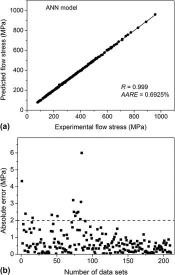
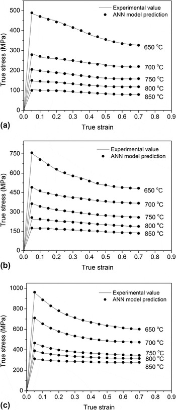
Figure 11 compares the experimental flow stress with the predicted values obtained from the developed ANN model. In which, nearly all data points are laid on the line inclined at 45° with an R value of 0.999. The AARE value is calculated as 0.6925%, much lower than that of both the Arrhenius type and multiple-linear models. Figure 11(b) shows the absolute error between the experimental and predicted values. The 93.81% of absolute errors are found to be less than 2 MPa. Figure 12 presents the comparative plots for the experimental and predicted flow stress values obtained from the ANN model, revealing the satisfactory predicted results of the developed ANN model in contrast to both the Arrhenius type and multiple-linear models.
Evaluation of the performance of developed ANN model: (a) correlation between the experimental and predicted flow stress, and (b) absolute error between the experimental and predicted values.

Comparison between experimental and predicted flow stress at various strain rates of (a) 0.01 s−1, (b) 0.1 s−1, and (c) 1 s−1 by using the ANN model.

The accuracy of these three constitutive equations was further investigated by the statistical analysis of relative errors between the experimental and predicted values, which were calculated by Eq. (16):
 $${\rm{Relative}}\;{\rm{error}} = \left( {{{{E_i} - {P_i}} \over {{E_i}}}} \right) \times 100\% \quad .$$
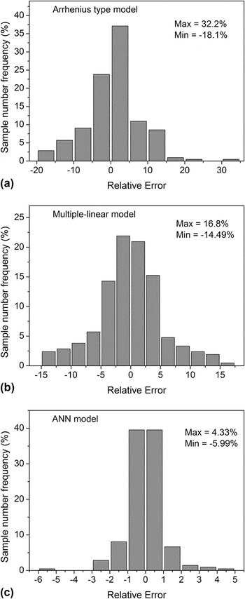
The statistical analysis results were depicted as the sampler number frequency versus relative error plot, as shown in Fig. 13. It can be seen that the relative errors obtained from the Arrhenius type model and the multiple-linear model are in the range of −18.1 to 32.2% and in the range of −14.49 to 16.8%, respectively, whereas those are found to vary from −5.99 to 4.33% for the ANN model. Moreover, the relative error within ±1% was shown for more than 79.05% of the test data sets of the ANN model, while only 10.0 and 17.62% of the test data sets for the Arrhenius type model and the multiple-linear model, respectively, which reveals the higher accuracy of the ANN model to characterize the hot deformation behavior of the as-forged Nitinol 60 alloy.
Statistical analysis of relative error by (a) Arrhenius type model, (b) multiple-linear model, and (c) ANN model.

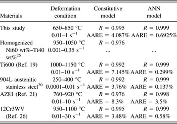
The low predictability of both the Arrhenius type and multiple-linear models indicates the response of deformation behavior under elevated temperatures and strain rates is nonlinear. Comparatively, the ANN is particularly more efficient than the constitutive equations, because no material constant is involved there. Table III summarized the predictability of the flow stress by the constitutive equations and the ANN model of various materials. By the analysis of statistical parameters (such as R and AARE), it seems that the new developed ANN model is much better.
The predictability of flow stress by the constitutive models and ANN model of various materials.

IV. CONCLUSIONS
A comparative study has been made on the ability of constitutive equations and ANN model to describe the elevated temperature flow behavior of the as-forged Nitinol 60 alloy investigated in the temperature range of 650–850 °C under the strain rate of 0.01–1 s−1. Based on the analysis done, the following conclusions can be made:
-
(1) Deformation temperature and strain rate have a strong influence on flow stress. The results indicate that the flow stress of the alloy increases with the increase of strain rate and the decrease of deformation temperature.
-
(2) The R and AARE values for the Arrhenius type model are found to be 0.989 and 5.661%, respectively, whereas those for the multiple-linear model are 0.995 and 4.087%, respectively. The relative errors obtained from the Arrhenius type model are in the range of −18.1 to 32.2%, whereas those are found to vary from −14.49 to 16.8% for the multiple-linear model. The multiple-linear model shows a higher accuracy in tracking the flow behavior of the as-forged Nitinol 60 alloy.
-
(3) The R and AARE values for the ANN model are 0.999 and 0.6925%, respectively. Also, the relative errors obtained from the ANN model vary from −5.79 to 4.33%. Moreover, the relative error within ±1% is observed for more than 79.05% of the test data sets of the ANN model, while only 10 and 17.62% of the test data sets for the Arrhenius type model and the multiple-linear model. Therefore, the ANN model has a better prediction power for the as-forged Nitinol 60 alloy than both the Arrhenius type model and multiple-linear model.
ACKNOWLEDGMENTS
We would like to thank our anonymous reviewers for extremely helpful comments. We acknowledge the support from the National Natural Science Foundation of China (Grant No. 51164030) and Natural Science Foundation of Jiangxi Province (Grant No. 20122 BAB216018).