


1. INTRODUCTION
Scheduling to minimize both earliness and tardiness (E/T) penalties has emerged to be a main thrust of research in the scheduling field. Investigations of these problems have largely been motivated by the adoption of the just-in-time concept in the manufacturing industry, which aims to complete jobs exactly at their due dates, not earlier and not later. There are, however, many other applications that espouse the concept of earliness–tardiness minimization. One example is the harvest of agricultural products, which should be conducted around their ripe times (due dates). Another example is the production and delivery of fresh products such as meat or dairy products. Such a product should not be finished too early, in order to avoid its possible decay, and should not be completed too late, in order to meet the customer demand.
As indicated in Baker and Scudder [3] a basic model of E/T scheduling is to minimize

where αi and βi are the unit costs due to earliness and tardiness of job i, respectively, Di is the due date of job i, and Ci is its completion time under a given schedule λ. This model has been extensively studied in the deterministic scheduling area and widely used as a canonical model in the E/T scheduling literature. See, for example, Garey, Tarjan, and Wilfong [15], Hall and Posner [16], Kovalyov and Kubiak [18], and Sen, Sulek, and Dileepan [24].
In sharp contrast with the deterministic case, however, progress on the stochastic counterpart of the above canonical model is still limited. Forst [12] appears to be the first one to deal with the problem. Under the condition that all processing times are independent and identically distributed (i.i.d.), he identified some special situations in which optimal monotone sequences with respect to {αi} or {βi} can be found. He concluded with the remark that “solving the general stochastic E/T problem … appears to be a very mathematically formidable task.” Soroush and Fredendall [25] considered the problem with symmetric E/T costs (i.e., αi = βi for all i) and Normally distributed processing times Pi. They obtained a deterministic equivalent, which becomes, however, a complicated, highly nonlinear function. Based on the central limit theorem, Cai and Zhou [7] addressed the situation where a job consists of a number elementary parts and thus the processing times of the jobs follow Normal distributions with variances proportional to means. They studied the problem with αi = α and βi = β for all i (but α might differ from β) and found a number of optimality properties and proposed a pseudopolynomial algorithm. Jia [17] considered the problem with αi = βi and Di = d for all i, where processing times Pi and the common due date d are exponentially distributed. He showed that the optimal sequence is Λ-shaped with respect to {wi /E(Pi)}. This result is extended to the case with machine breakdowns when the uptimes and downtimes are exponentially distributed. Qi, Yin, and Birge [23] studied a problem with linear E/T functions. Sufficient conditions to ensure an optimal SEPT (shortest expected processing time) sequence are developed. Some further results are also obtained when processing times follow exponential and normal distributions.
A related E/T scheduling model deals with quadratic penalty functions (i.e., to minimize [sum ][αi(max{0,Di − Ci})2 + βi(max{0,Ci − Di})2]). There has been considerable progress achieved on the stochastic variants of this quadratic E/T scheduling model; see, for example, Chakravarthy [10], Vani and Raghavachari [26], Mittenthal and Raghavachari [20], Cai and Tu [6], Luh, Chen, and Thakur [19], and Cai and Zhou [9]. To a certain extent, the quadratic model is relatively easy to handle in stochastic settings, because of the differentiability associated with the squared cost functions. The model with a piecewise linear objective function as in (1.1), on the other hand, does not enjoy such a convenience and becomes more complicated when stochastic variables such as random processing times and machine breakdowns are taken into account.
In this article we study the stochastic E/T scheduling problem under the following settings: (1) The objective is to minimize the expected total cost (1.1), where αi and βi might be different; (2) jobs have random processing times and due dates, which are independently and exponentially distributed; (3) the machine is subject to stochastic breakdowns, with the uptimes following an exponential distribution and the downtimes (repair times) following a general distribution. Note that in problems with regular objective functions,1
An objective function is said to be regular if it is a nondecreasing function of the completion time of any job. An objective function involving an earliness cost is nonregular, since it might decrease as the completion time increases.
We consider, in this article, both preempt-resume and preempt-repeat breakdown models (see, e.g., Birge, Frenk, Mittenthal, and Rinnoog Kan [4]). Under the preempt-resume model, it is assumed that if a machine breakdown occurs during the processing of a job, the work done on the job prior to the breakdown is not lost and the processing of the disrupted job can be continued from where it was interrupted. The preempt-repeat model, on the other hand, assumes that the work done prior to a breakdown is lost and the processing of the job will have to be redone again when the machine resumes operation. This is generally a much more difficult model (see Cai, Sun, and Zhou [5]), on which little has been found in the E/T scheduling literature. In our model considered in this article, however, the two breakdown models are actually equivalent (see Section 2.2).
The main contributions of our study in this article are as follows:
- We derive several sufficient conditions under which the optimal
sequence is V-shaped2with respect to {E(Pi)/αi}, or {E(Pi)/βi}, or both. The V-shaped structure of optimal solutions is an important characteristic that exists in some E/T scheduling problems (see, e.g., Eilon and Chowdhury [11] and Mittenthal and Raghavachari [20]), which makes it possible to develop efficient algorithms based on dynamic programming.
A sequence is V-shaped with respect to {ai}, where ai is an attribute of job i, i = 1,2,…, n, if it first arranges jobs in a nonincreasing order of {ai} and then in a nondecreasing order of {ai}.
- We derive a number of sufficient conditions under which optimal solutions can be constructed analytically.
- We also present an algorithm that computes the best V-shaped sequence using dynamic programming.
The article is organized as follows. In Section 2 we describe the basic problem, the assumptions, and the breakdown models. The results on optimal V-shaped sequences are presented in Section 3. In Section 4 we identify several conditions under which optimal sequences can be constructed analytically. A dynamic programming algorithm to obtain the best V-shaped sequence is provided in Section 5. Finally, some concluding remarks are discussed in Section 6.
2. PROBLEM STATEMENT
Consider the problem where a set of n jobs are to be processed by a single machine. All jobs are ready for processing at time t = 0. The processing times Pi of job i, i = 1,2,…, n, are random variables, which are independently and exponentially distributed with means μ1,…, μn, respectively. Each job i has a due date Di, and D1,…, Dn are independently and exponentially distributed with a common mean 1/δ, independent of {Pi}. Job preemption is not allowed; that is, if a job has been started, it has to be processed on the machine until it is completed.
The machine is subject to random breakdowns. The breakdown process of the machine is characterized by a sequence of finite-valued, positive random vectors {Yk,Zk}k=1∞, where Yk and Zk represent the durations of the kth uptime and the kth downtime, respectively. If a machine breakdown occurs during the processing of a job, the work done on the job prior to the breakdown might follow either a preempt-resume model or a preempt-repeat model, depending on the nature and the processing requirements of the jobs. More details on the two breakdown models will be further elaborated in Sections 2.1 and 2.2. For the breakdown process of the machine, we make the following assumptions:
- The breakdown process is independent of the processing times {Pi} and the due dates {Di}.
- {Yk,Zk}k=1∞ is a sequence of i.i.d. random vectors.
- The uptimes {Yk} of the machine are exponentially distributed with mean 1/τ, the downtimes {Zk} follow a general common distribution with mean ν, and the {Yk} are independent of {Zk}.
The problem is to determine an optimal sequence to process all jobs, so as to minimize the expected total earliness and tardiness cost:

where
- λ = (i1,i2,…, in) is a job sequence, which is a permutation of {1,2,…, n} that determines the order to process the n jobs, with ik = j if and only if job j is the kth to be processed;
- Ci = Ci(λ) is the completion time of job i under sequence λ;
- αi is the unit earliness cost to job i;
- βi is the unit tardiness cost to job i;
- D is a representative of due dates {Di}; in other words, an exponentially distributed random variable with mean 1/δ, independent of {Pi};
- E[X] denotes the expectation of a random variable X;
- IA is the indicator of an event A that takes the value 1 if A occurs and is zero otherwise.
We assume that the machine will start its first job at time 0, although this assumption is not necessary (see also remarks in Section 6).
The impact of machine breakdowns on job processing can follow the following two models.
2.1. The Preempt-Resume Model
Under this model, if a machine breakdown occurs during the processing of a job, the work done on the job prior to the breakdown is not lost and the processing of the disrupted job can be continued from the point where it was interrupted (cf. Birge et al. [4]).
Define a counting process N(t) = sup{k ≥ 0 : Sk ≤ t}, where Sk = Y1 + Y2 + ··· + Yk denotes the total uptime of the machine before its kth breakdown (with S0 = 0). By the assumption that the {Yk} are exponentially distributed with mean 1/τ, N(t) is a Poisson process with rate τ.
Let

denote the set of jobs sequenced no later than job i under λ. Then the completion time of job i under λ can be expressed as

where

represents the total uptime of the machine before job i is finished and Z0 ≡ 0.
2.2. The Preempt-Repeat Model
In this model, if the machine breakdown occurs during the processing of a job, the work done on this job is lost and the processing will have to be done for this job all over again after the machine resumes its work (cf. Birge et al. [4]).
As in the previous literature (e.g., Frostig [14]), we assume that each time that a job is repeated, the processing time required is resampled independently according to its probability distribution. Then there is a sequence of independent processing times {Pik}k=0∞ to process job i, and each Pik is a replicate of Pi, exponentially distributed with mean μi.
In general, the impact of preempt-repeat breakdowns can differ significantly from that of preempt-resume breakdowns. However, if the processing times are exponential, then due to the memoryless property of the exponential distribution, the remaining processing time at a breakdown has the same distribution as the original processing time, given that the job has not been completed. Thus, the two breakdown models become equivalent. As a result, we only need to consider the preempt-resume model for machine breakdowns, which will be assumed throughout the rest of the article.
3. V-SHAPED OPTIMAL SEQUENCES
We first derive an equivalent form of the objection function defined in (2.1), which is given in the following theorem.
Theorem 1: Under the preempt-resume model,

where

and

Proof: By the independence between the processing times, the due dates, and the machine breakdowns, we have

Hence,

Furthermore, as D is exponentially distributed, by (2.2) and (2.3) we have

It follows that

Substituting (3.6) into (3.4), we obtain

Similarly, we can calculate

Hence,

Since

it follows from (2.2), (3.9), and the assumptions on Pk, N(t), and Zk that

Substituting (3.10) and (3.6) into (3.8), we get

which together with (3.7) gives (3.1). █
In what follows we will suppress λ from

for ease of notation. Define

Then (3.1) can be rewritten as

The next theorem is one of our main results, which shows that the optimal sequence is V-shaped with respect to {μi /βi} under appropriate conditions.
Theorem 2: Define

If {γij} satisfy

for all distinct i,j,k ∈ {1,…, n} such that γjk and γij are defined, then an optimal sequence λ* that minimizes ETC(λ) is V-shaped with respect to {μi /βi}.
Proof: Given two jobs i and j, consider two sequences: λ = {…,i,j,…} and λ′ = {…,j,i,…}; that is, λ and λ′ are identical except the order of jobs i and j is switched. Let

denote the set of jobs to be processed just before i and j under either λ or λ′. Then by (3.12),

Furthermore, by (3.2) we have

Hence,

Combining (3.16) and (3.18) with (3.13), we obtain

By (3.14), (3.19) can be written as

Now let λ be an arbitrary sequence that is not V-shaped with respect to {μi /βi}. Without loss of generality, we can assume that λ = {1,2,…, n}. Then there are three consecutive jobs i, i + 1, and i + 2 under λ such that

or, equivalently,

Let λ1 denote the sequence that switches jobs i and i + 1 in λ, and λ2 the sequence that switches jobs i + 1 and i + 2 in λ so that

and

By (3.20),

where

Similarly,

By condition (3.15), either

or

If Ai < 0, then by (3.21) and (3.22), ETC(λ) − ETC(λ1) > 0. When Ai ≥ 0, by (3.23) and (3.25), either

or Ai+1 > 1 + ντ − (1 + γi+1,i+2)η/δ > 0. Therefore, ETC(λ) − ETC(λ2) > 0 by (3.21) and (3.24). In either case, λ cannot be an optimal sequence. Thus, an optimal sequence must be V-shaped with respect to {μi /βi}. █
If γij ≥ 0 for all i,j, then {μi /αi} have the same order as {μi /βi}. Hence, we have the following result on the V-shape property of the optimal sequence with respect to {μi /αi}.
Corollary 1: If γij ≥ 0 for all i and j and condition (3.15) holds for γij > 0 and γjk > 0, then an optimal sequence λ* that minimizes ETC(λ) is V-shaped with respect to {μi /αi} (as well as to {μi /βi}).
On the other hand, if γij ≤ 0 for all i and j, then {μi /αi} and {μi /βi} have opposite orders. In such a case, an analytic solution is available. This result will be given in Theorem 3 in Section 4. Here we continue our analysis of V-shaped sequences.
Remark 1: When γij > 0 for some i and j and γij < 0 for other i and j, it is possible that an optimal sequence is V-shaped with respect to {μi /βi}, but not to {μi /αi}. See the following example.
Example 1: Let n = 3, μ1 = μ2 = μ3 = 1, (β1,β2,β3) = (4,3,1), (α1,α2,α3) = (2,1,2), and η = 4. Then it is not difficult to see that

so that

hence, (3.15) holds. Following Corollary 4 in Section 4, we will show that the optimal sequence is λ* = (1,2,3), which is in nondecreasing order of (hence V-shaped with respect to)

, but not V-shaped with respect to

.
We now look at some special cases in which condition (3.15) holds.
Case I: {(αj /μj) − (αi /μi)} and {(βj /μj) − (βi /μi)} are proportional; that is,

for some constant K. Then γij ≡ K. When K > 0, {αi /μi} and {βi /μi} have the same order and condition (3.15) holds obviously. If K ≤ 0, then {αi /μi} and {βi /μi} are in opposite orders. Thus, Theorems 1 and 2 lead to the following corollary.
Corollary 2: If (3.26) holds for some constant K, then an optimal sequence λ* that minimizes ETC(λ) is V-shaped with respect to both {μi /βi} and {μi /αi}.
Remark 2: If {αi} and {βi} are proportional (i.e., αi = cβi, i = 1,…, n, for some constant c), then (3.26) holds with K = c. Hence, Corollary 2 covers this case. In particular, when αi = βi, i = 1,…, n, the objective function in (2.1) becomes

Hence, the main results of Jia [17] are a special case of our Corollary 2.
Case II: {(αj /μj) − (αi /μi)} and {(βj /μj) − (βi /μi)} are not equal, or proportional, but are close to each other in the sense that

where |εij| ≤ ε < 2 for all i,j. Then γij = 1 + εij and so

Furthermore, if ε < 1, then γij > 0 for all i and j, so that {μi /βi} and {μi /αi} have the same order. Thus, we obtain the following corollary.
Corollary 3: If (3.27) holds with

then an optimal sequence λ* to minimize ETC(λ) is V-shaped with respect to {μi /βi}. If, in addition, ε < 1, then λ* is also V-shaped with respect to {μi /αi}.
Remark 3: Although the above theorem and corollaries cover a fairly wide range of parameters such that an optimal sequence is V-shaped with respect to {μi /βi} or {μi /αi} (or both), there are certainly situations in which the optimal sequence does not have a V-shape with respect to {μi /βi} or {μi /αi}. On the other hand, the conditions in each theorem or corollary are sufficient only, and there might exist a V-shaped optimum even though these conditions are not satisfied. See the following examples.
Example 2: Let n = 3, μ1 = μ2 = μ3 = 1, (β1,β2,β3) = (2,1,2), (α1,α2,α3) = (3,1,9), δ = 1, and τ = 0. Then fi = ½, i = 1,2,3. By (3.1), the objective function in this case is given by

Simple calculations show that

Thus, the optimal sequence is λ* = (1,2,3), which is not V-shaped with respect to

or to

.
Example 3: Let n = 3, μ1 = μ2 = μ3 = 1, (β1,β2,β3) = (6,4,2), (α1,α2,α3) = (1,3,2), δ = 1, and τ = 0. Then

. Hence,

Therefore, the conditions of Theorem 2 do not hold. However, it is easy to verify that the conditions of Theorem 4 or Corollary 4 (see Section 4) hold, and so the optimal sequence is λ* = (1,2,3), which is not only nondecreasing in

but also V-shaped with respect to

.
4. ANALYTICAL OPTIMAL SEQUENCES
We will reveal, in this section that there exist analytical optimal solutions for the problem if certain conditions are satisfied. The following theorem is one of our main results.
Theorem 3: If {μi /βi} and {μi /αi} have opposite orders, that is,

then a sequence in nondecreasing order of {μi /βi} or in nonincreasing order of {μi /αi}, is optimal to minimize ETC(λ).
Proof: Let βj /μj ≥ βi /μi so that αj /μj ≤ αi /μi by the condition of the theorem. Since

it follows from (3.19) that ETC(λ) ≥ ETC(λ′). Thus, ETC(λ) ≥ ETC(λ′) if and only if βj /μj ≥ βi /μi or μj /βj ≤ μi /βi. The theorem then follows. █
In addition to Theorem 3, there are a number of other situations in which an analytic solution is available to minimize ETC(λ), as shown below.
Without loss of generality we assume μ1 ≤ μ2 ≤ ··· ≤ μn in Theorem 4.
Theorem 4: If

where

for all i,j = 1,…, n, then a sequence in nondecreasing order of {μi /βi} is optimal to minimize ETC(λ).
Proof: Under the conditions of the theorem,

Hence, by (3.20), ETC(λ) ≥ ETC(λ′) if and only if

This shows that an optimal sequence should schedule job j ahead of job i if μj /βj ≤ μi /βi. The theorem follows. █
Since η ≤ δ(1 + τν), we have B ≥ (1 + ημ1)(1 + ημ2) − 1 > η(μ1 + μ2), which leads to the next corollary.
Corollary 4: If

then a sequence in nondecreasing order of {μi /βi} minimizes ETC(λ).
Example 1 (continued): Let n = 3, μ1 = μ2 = μ3 = 1, (β1,β2,β3) = (4,3,1), (α1,α2,α3) = (2,1,2), and η = 4. Then
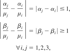
and η(μ1 + μ2) = 4(1 + 1) = 8. Hence, the condition of Corollary 4 holds and so λ* = (1,2,3) is the optimal sequence.
As a special case of Corollary 4, we have the following corollary.
Corollary 5: If {αi} are proportional to {μi} (i.e., αi = cμi, i = 1,…, n, for some constant c), then a sequence in nondecreasing order of {μi /βi} minimizes ETC(λ).
Theorem 5: If

where

for all i,j = 1,…, n, then a sequence in nonincreasing order of {μi /αi} is optimal to minimize ETC(λ).
Proof: By the definition of

,

Let

or, equivalently,

Then by (3.19) and (4.1) together with the conditions of the theorem,

Thus, an optimal sequence should place job i ahead of job j if μj /αj ≤ μi /αi. This proves the theorem. █
A special case of Theorem 5 is given next.
Corollary 6: If {βi} are proportional to {μi}, then a sequence in nonincreasing order of {μi /αi} minimizes ETC(λ).
5. AN ALGORITHM TO COMPUTE THE BEST V-SHAPED SEQUENCE
In this section we provide an algorithm that can search the best V-shaped sequence among all V-shaped sequences. Without loss of generality, we assume that the jobs have been numbered such that μ1 /β1 ≤ μ2 /β2 ≤ ··· ≤ μn /βn.
Consider a set of jobs Si = {1,2,…, i}. In a V-shaped sequence, job i will be sequenced either the first or the last among all jobs in Si. Assume that λ* is the best V-shaped sequence and Si is the set of jobs sequenced before all jobs in Si under λ*, and let

Define hi(Θi,Ψi) to be the contribution of all jobs in Si to the cost function (3.1), given Θi and Ψi. Then it is easy to see that the costs arising from sequencing job i as the first and the last job among all jobs in the set Si will be respectively

and

It follows from the principle of optimality of dynamic programming that, with hia(Θi,Ψi) and hib(Θi,Ψi) defined above, the best V-shaped sequence λ* must sequence job i such that

We therefore have the following algorithm.
Algorithm 1
- For i = 1,2,…, n, compute hi(Θi,Ψi) according to (5.2), for all possible values in the feasible sets of Θi and Ψi.
- Let Hn* = minΘn,Ψn{hn(Θn,Ψn)}.
- Construct, by a backward tracking process, the sequence λ* that achieves Hn*.
We have omitted the details of the backward tracking process to find λ*. We have also omitted the definitions of the feasible sets for Θi and Ψi defined in (5.1). With certain assumptions (e.g., all μi are integers), one can identify finite feasible sets for Θi and Ψi, and the time complexity of Algorithm 1 might become pseudopolynomial.
6. CONCLUDING REMARKS
We have studied the stochastic scheduling problem with asymmetric linear E/T costs, a canonical model in the E/T scheduling literature. This model is regarded as rather difficult since the piecewise linear nature of its objective function complicates the analysis of optimal solutions. A significant advancement achieved in this article is the finding of a number of propositions regarding the optimal solutions under the settings of exponential processing times and exponential due dues. We have found that these propositions remain valid for fairly general machine breakdown processes, where the uptimes follow an exponential distribution and downtimes (repair times) can follow any general distribution, and the machine breakdowns can be of either preempt-resume or preempt-repeat patterns. Note that an uptime lasts until a machine breakdown occurs. Since the occurring time of a breakdown is usually quite uncertain, using an exponential distribution to model it is reasonable. The repair time, on the other hand, can depend on various factors, such as the severity of the machine breakdown, the amount of time needed to diagnose the cause of the failure, and the available expertise and manpower, and, therefore, a general distribution is obviously more desirable.
We have obtained sufficient conditions for the optimal sequences to be V-shaped or analytical. An algorithm has also been provided to show how the best V-shaped sequence can be computed using dynamic programming.
Although we have assumed that the machine will start the first job at time 0, all of our results obtained in this article can be generalized to allow a nonzero machine start time. Extensions to include other types of costs (such as a weighted flow time) are also possible.
The complexity of the problem in terms of NP-completeness remains an open question. We conjecture that it is NP-complete in the ordinary sense, under the sufficient conditions that we have derived here to ensure a V-shaped optimal sequence and with certain assumptions such as integer-valued μi. Another interesting future work is to look at the possibility of generalizing the results in this article to situations involving nonexponential processing times, with the objective of finding approximate solutions.
Acknowledgments
The authors are grateful to an anonymous referee whose valuable suggestions and comments have helped improve the article.
This work was partially supported by the Research Grants Council of Hong Kong under Earmarked grants CUHK 4166/01E and 4170/03E and PolyU5142/01E and 5146/02E, and NSFC Research Fund No. 70329001 and 70518002.


