1. Introduction
Instabilities in shear-dominated flows have been observed in many industrial, geophysical and astrophysical flows. The instabilities in geophysical flows are of interest due to the wide array of remarkable patterns that form on Earth and extraterrestrial planets. The polygonal configurations observed in polar vortices, for instance, have been hypothesized to originate from barotropically unstable shear layers and jets (Aguiar Reference Aguiar2008; Aguiar et al. Reference Aguiar, Read, Wordsworth, Salter and Hiro Yamazaki2010; Montabone et al. Reference Montabone, Wordsworth, Aguiar, Jacoby, Manfrin, Read, Castrejon-Pita, Gostiaux, Sommeria, Viboud and Didelle2010). Polar vortices engender much interest since the origin, longevity, and the preferred state of their striking and unique polygonal structures are still not well understood, despite having been observed for decades (e.g. Taylor et al. Reference Taylor, Diner, Elson, McCleese, Martonchik, Delderfield, Bradley, Schofield, Gille and Coffey1979; Godfrey Reference Godfrey1988; Charlton et al. Reference Charlton, O’Neill, Lahoz and Berrisford2005; Piccioni et al. Reference Piccioni, Drossart, Sanchez-Lavega, Hueso, Taylor, Wilson, Grassi, Zasova, Moriconi, Adriani, Lebonnois, Coradini, Bezard, Angrilli, Arnold, Baines, Bellucci, Benkhoff, Bibring, Blanco, Blecka, Carlson, Di Lellis, Encrenaz, Erard, Fonti, Formisano, Fouchet, Garcia, Haus, Helbert, Ignatiev, Irwin, Langevin, Lopez-Valverde, Luz, Marinangeli, Orofino, Rodin, Roos-Serote, Saggin, Stam, Titov, Visconti and Zambelli2007; Fletcher et al. Reference Fletcher, Irwin, Orton, Teanby, Achterberg, Bjoraker, Read, Simon-Miller, Howett, de Kok, Bowles, Calcutt, Hesman and Flasar2008).
The pursuit of understanding these planetary-scale polygonal structures has been supported by theoretical, numerical and experimental studies of an unstable Stewartson layer. Stewartson layers can exist at the interface between concentric bodies of fluid rotating at different speeds. The layers are a nested structure composed of a thick and thin layer, both serving different functions (Stewartson Reference Stewartson1957; Smith Reference Smith1984). Experimental techniques in particular have been popular in investigating these rotating flows due to the relatively simple reproduction of the instabilities in the laboratory. The range of apparatus used to investigate these layers include cylindrical containers with both flat (Hide & Titman Reference Hide and Titman1967; Rabaud & Couder Reference Rabaud and Couder1983; Chomaz et al.
Reference Chomaz, Rabaud, Basdevant and Couder1988; Früh & Read Reference Früh and Read1999; Bergeron et al.
Reference Bergeron, Coutsias, Lynov and Nielsen2000) and varying bottom topographies (van de Konijnenberg et al.
Reference van de Konijnenberg, Nielsen, Juul Rasmussen and Stenum1999; Aguiar Reference Aguiar2008; Aguiar et al.
Reference Aguiar, Read, Wordsworth, Salter and Hiro Yamazaki2010), and spherical shells (Hollerbach Reference Hollerbach2003; Hollerbach et al.
Reference Hollerbach, Futterer, More and Egbers2004; Schaeffer & Cardin Reference Schaeffer and Cardin2005). All of these set-ups involve mechanically induced differential rotation, which generates Stewartson layers that are susceptible to instability. Despite the differences in configuration, these studies have illustrated polygonal structures via an unstable Stewartson layer which are similar in appearance to planetary polar vortices. However, there are subtleties inherent in the type of configuration which can influence the flow dynamics. For example, Hollerbach (Reference Hollerbach2003) concluded that the anomalous states between positive-
 $\mathit{Ro}$
and negative-
 $\mathit{Ro}$
flows observed by Hide & Titman (Reference Hide and Titman1967) was due to the abrupt change in depth across the Stewartson layer caused by the geometry of the system.
Experimental results have largely revealed the trends in the preferred azimuthal states of these flows as functions of non-dimensional parameters. However, limitations of these experiments include difficulty visualizing the vertical structure of the non-axisymmetric flow, measuring certain flow parameters, and identifying underlying structures. As such, numerical studies have been complementary in the fundamental understanding of the flow structure (e.g. Bergeron et al. Reference Bergeron, Coutsias, Lynov and Nielsen2000; Früh & Nielsen Reference Früh and Nielsen2003; Schaeffer & Cardin Reference Schaeffer and Cardin2005). Until recently, numerical efforts have been restricted to quasi-two-dimensional modelling since full three-dimensional simulations are computationally intensive. Hence, numerical studies are yet to elucidate the vertical structure of the flow. In addition, comparisons between experimental observations and numerical results have exhibited discrepancies. The unresolved depth-dependent structures such as the thin inner Stewartson layer, which is responsible for completing the meridional circulation induced by the Ekman layers, are often referenced as being the reason for the differences (Früh & Read Reference Früh and Read1999; van de Konijnenberg et al. Reference van de Konijnenberg, Nielsen, Juul Rasmussen and Stenum1999). Despite these limitations, vortical structures that resemble those of natural axial vortices have been successfully recreated (Aguiar et al. Reference Aguiar, Read, Wordsworth, Salter and Hiro Yamazaki2010; Montabone et al. Reference Montabone, Wordsworth, Aguiar, Jacoby, Manfrin, Read, Castrejon-Pita, Gostiaux, Sommeria, Viboud and Didelle2010).
This paper considers a cylindrical container with differential rotation forced by coaxial disks to generate Stewartson layers. That is, two different angular velocities are forced about the same axis of rotation. It should be noted that other planetary phenomena have been investigated using configurations with multiple angular velocities with a time dependence and rotation about multiple axes. Such flows are known as librating (e.g. Noir et al. Reference Noir, Calkins, Lasbleis, Cantwell and Aurnou2010; Lopez & Marques Reference Lopez and Marques2011; Koch et al. Reference Koch, Harlander, Egbers and Hollerbach2013) and precessing (e.g. Kobine Reference Kobine1995; Kong, Liao & Zhang Reference Kong, Liao and Zhang2014; Kong et al. Reference Kong, Cui, Liao and Zhang2015) flows. These characteristics mimic several planets within our solar system possessing longitudinal libration and an interior dynamo. Furthermore, a precession-driven flow would naturally occur in laboratory experiments since the rotation axis of the system does not often align with the rotation axis of the Earth. Thus, understanding the effect of the precession may have significant implications for investigating rotating flows (see Boisson et al. Reference Boisson, Cébron, Moisy and Cortet2012; Triana, Zimmerman & Lathrop Reference Triana, Zimmerman and Lathrop2012, and references therein). Despite the existence of Stewartson and Ekman layers in these flows, these shear and boundary layers are often not the primary flow driver. Hence, inertial waves are typically of interest in these unstable librating and precessing flows (e.g. Manasseh Reference Manasseh1992; Meunier et al. Reference Meunier, Eloy, Lagrange and Nadal2008; Calkins et al. Reference Calkins, Noir, Eldredge and Aurnou2010; Sauret et al. Reference Sauret, Cébron, Le Bars and Le Dizès2012). In contrast, this paper examines the non-axisymmetric structure of the unstable Stewartson shear layer responsible for the polygonal deformations in both the linear and nonlinear growth regimes.
Vo, Montabone & Sheard (Reference Vo, Montabone and Sheard2014) were the first to characterize the vertical structure of the axisymmetric base flow and identify azimuthal linear instability modes that can cause polygonal deformations to the Stewartson layer. These shear layers were produced by the differential rotation of disks in a rotating cylindrical tank. The azimuthal linear instabilities of primary importance were named mode I and mode II. The primary difference between the two modes is that mode I disturbance structures extend through the interior in the vicinity of the Stewartson layer leading to its distortion and formation of polygonal shapes, while mode II structures are localized near the base and lid in the vicinity of the disk–tank interface. Thus, the mode I instability was the mode of interest due to the similar traits it displayed with respect to barotropic instability. Additionally, the mode I instability was observed to favour low-wavenumber structures, which are in line with the range of patterns observed in nature such as Saturn’s north pole and Venus’s south pole. A third instability mode, mode III, was also identified at flows characterized by larger Reynolds numbers. It was proposed that the mode I instability was associated with the unstable
 $\mathit{Ek}^{1/4}$
Stewartson layer while the mode II instability was associated with the symmetry breaking of the flow about the mid-depth (i.e. the
 $\mathit{Ek}^{1/3}$
layer). This hypothesis was supported by Vo, Montabone & Sheard (Reference Vo, Montabone and Sheard2015), who recently studied the linear stability of the same flow in various aspect ratios using axisymmetric and quasi-two-dimensional models. The numerical analysis from both of those studies considered axisymmetric flow and linear non-axisymmetric disturbances, whereas nonlinear aspects of the instability mode evolution and the consistency between saturated non-axisymmetric flows and quasi-two-dimensional model predictions have yet to be explored.
This paper examines the non-axisymmetric structures produced in an unstable differentially rotating flow using full three-dimensional direct numerical simulation and a quasi-two-dimensional model. Comparisons between the two methodologies are performed and the validity of the quasi-two-dimensional model is discussed. The significance of the most unstable azimuthal linear instabilities predicted by linear stability analysis (Vo et al. Reference Vo, Montabone and Sheard2014) is explored by resolving the three-dimensional flow in regimes both near and well beyond the onset of instability. This investigation stems from the unexplained discrepancies observed in the azimuthal wavenumbers obtained experimentally by Früh & Read (Reference Früh and Read1999) to those predicted by linear stability analysis (Vo et al. Reference Vo, Montabone and Sheard2014). The results will elucidate the effects of nonlinearity and temporal behaviour in these flows. This paper further investigates the sensitivity of the three-dimensional flow to initial conditions which may, in part, explain the longevity of various polar vortical structures.
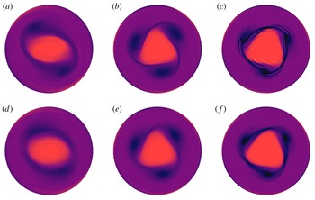
This paper is organized as follows. The numerical methodology is outlined in § 2, which includes a description of the system, the governing parameters, and the two numerical models. Results of the non-axisymmetric flows are described in § 3, including three-dimensional modelling of flows in the vicinity of instability onset (§ 3.1), flows well beyond the instability onset (§ 3.2), and the flow sensitivity and its transition characteristics (§ 3.3). Section 3.4 examines the corresponding non-axisymmetric flows using a quasi-two-dimensional model. Finally, the key conclusions are drawn in § 4.
2. Methodology
2.1. System description and governing parameters
The system studied in this paper consists of a cylindrical tank rotating at angular speed
 ${\it\Omega}$
with differential rotation imparted by disks located at the lid and base of the tank. This configuration has been studied previously by numerous authors (e.g. Früh & Read Reference Früh and Read1999; Aguiar Reference Aguiar2008; Vo et al.
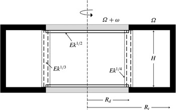
Reference Vo, Montabone and Sheard2014, Reference Vo, Montabone and Sheard2015) and a schematic of the system is shown in figure 1. The key dimensions adopted here match the physical proportions used by Früh & Read (Reference Früh and Read1999) such that the ratio of the disk and tank radii is
 $R_{d}/R_{t}=1/2$
and the aspect ratio (ratio of the tank height to disk radius) is
 $A=H/R_{d}=2/3$
.
A schematic diagram of the differential rotating disk set-up under investigation. The key dimensions are the disk radius
 $R_{d}$
, tank radius
 $R_{t}$
, and tank height
 $H$
. The disks and tank rotate about the central axis (thin dashed line) at a rate of
 ${\it\Omega}+{\it\omega}$
and
 ${\it\Omega}$
, respectively. Boundary and shear layers are also shown, where vertical lines represent the Stewartson layers (and their thickness scalings with Ekman number as
 $\mathit{Ek}^{1/4}$
and
 $\mathit{Ek}^{1/3}$
) and horizontal lines represent the Ekman layers (
 $\mathit{Ek}^{1/2}$
thickness scaling).

In the inertial frame of reference, the time-dependent incompressible Navier–Stokes equations governing the flow of a Newtonian fluid are
 $$\begin{eqnarray}\displaystyle & {\displaystyle \frac{\partial \boldsymbol{u}}{\partial t}}+(\boldsymbol{u}\boldsymbol{\cdot }\boldsymbol{{\rm\nabla}})\boldsymbol{u}=-{\displaystyle \frac{1}{{\it\rho}}}\boldsymbol{{\rm\nabla}}p+{\it\nu}{\rm\nabla}^{2}\boldsymbol{u}, & \displaystyle\end{eqnarray}$$
 $$\begin{eqnarray}\displaystyle & \boldsymbol{{\rm\nabla}}\boldsymbol{\cdot }\boldsymbol{u}=0, & \displaystyle\end{eqnarray}$$
 $\boldsymbol{u}$
is the velocity field,
 $p$
is the pressure,
 ${\it\rho}$
is the fluid density,
 ${\it\nu}={\it\mu}/{\it\rho}$
is the fluid kinematic viscosity and
 ${\it\mu}$
is the dynamic viscosity.
A number of dimensionless parameters characterize the flow, including the Rossby number
 $\mathit{Ro}$
, the Ekman number
 $\mathit{Ek}$
, and the internal Reynolds number
 $\mathit{Re}_{i}$
. These parameters characterize the importance of inertial forces, viscous forces, and Coriolis forces relative to one another, and are respectively defined as
 $$\begin{eqnarray}\displaystyle & \mathit{Ro}={\displaystyle \frac{R_{d}{\it\omega}}{2\overline{{\it\Omega}}H}}, & \displaystyle\end{eqnarray}$$
 $$\begin{eqnarray}\displaystyle & \mathit{Ek}={\displaystyle \frac{{\it\nu}}{\overline{{\it\Omega}}H^{2}}}, & \displaystyle\end{eqnarray}$$
 $$\begin{eqnarray}\displaystyle & \mathit{Re}_{i}={\displaystyle \frac{\sqrt{2}\mathit{Ro}}{\mathit{Ek}^{3/4}}}, & \displaystyle\end{eqnarray}$$
 $\overline{{\it\Omega}}={\it\Omega}+{\it\omega}/2$
is the appropriate mean rotation rate following Früh & Read (Reference Früh and Read1999) and Aguiar (Reference Aguiar2008). The internal Reynolds number is based on a Stewartson layer scaling with thickness
 $L=(\mathit{Ek}/4)^{1/4}H$
, and has been shown to be important in describing the onset of instability in this type of system (Niino & Misawa Reference Niino and Misawa1984; Früh & Read Reference Früh and Read1999; Vo et al.
Reference Vo, Montabone and Sheard2014, Reference Vo, Montabone and Sheard2015).
2.2. Numerical treatment
The length, velocity, time, and pressure dimensions in (2.1) are scaled by
 $R_{d}$
,
 $R_{d}{\it\Omega}$
,
 ${\it\Omega}^{-1}$
and
 ${\it\rho}(R_{d}{\it\Omega})^{2}$
, respectively, to derive the non-dimensional governing equations
 $$\begin{eqnarray}\displaystyle & {\displaystyle \frac{\partial \boldsymbol{u}}{\partial t}}+(\boldsymbol{u}\boldsymbol{\cdot }\boldsymbol{{\rm\nabla}})\boldsymbol{u}=-\boldsymbol{{\rm\nabla}}p+{\displaystyle \frac{\mathit{Ek}\,A^{2}}{1-A\mathit{Ro}}}{\rm\nabla}^{2}\boldsymbol{u}, & \displaystyle\end{eqnarray}$$
 $$\begin{eqnarray}\displaystyle & \boldsymbol{{\rm\nabla}}\boldsymbol{\cdot }\boldsymbol{u}=0. & \displaystyle\end{eqnarray}$$
Two different models have been employed to compute the non-axisymmetric flow structures in this paper. The first considers the full three-dimensional equations simulated via computationally expensive direct numerical simulation, and the second considers a simplified quasi-two-dimensional model described by two-dimensional equations with an added external forcing term. These two models are described separately in the following sections.
2.2.1. Spectral-element–Fourier technique
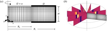
The geometry considered in this paper possesses an azimuthal homogeneity, and therefore an efficient approach to compute the non-axisymmetric flow in the geometry is to use a spectral-element–Fourier method (Blackburn & Sherwin Reference Blackburn and Sherwin2004). A spectral-element method is used to discretize the flow in the two-dimensional
 $r{-}z$
semi-plane (see figure 2
a). Boundary conditions are imposed such that the grey regions represent the disks which rotate at a rate of
 ${\it\Omega}+{\it\omega}$
, while the black regions represent the tank walls and rotate at a rate of
 ${\it\Omega}$
. On the symmetry axis, appropriate zero Dirichlet and Neumann conditions are imposed on the pressure and velocity component Fourier modes as detailed in Blackburn & Sherwin (Reference Blackburn and Sherwin2004). Axisymmetric steady-state base flows are prescribed as the initial condition for the three-dimensional simulations, unless stated otherwise.
(a) The spatially discretized semi-meridional
 $r{-}z$
plane used to simulate axisymmetric flows with macro elements shown. The disks (grey) and tank (black) boundaries rotate about the central axis (dashed line) at a rate of
 ${\it\Omega}+{\it\omega}$
and
 ${\it\Omega}$
, respectively. (b) An oblique view of the three-dimensional domain achieved via the azimuthal expansion (spectral-element–Fourier technique) of the semi-meridional mesh shown in (a). Several
 $r{-}z$
planes at different azimuthal angles are illustrated with contours of axial vorticity to demonstrate the non-axisymmetric nature of the flow.

The third dimension is constructed through a Fourier expansion of the velocity and pressure fields. In cylindrical coordinates, the two-dimensional
 $r{-}z$
plane is expanded in the azimuthal
 ${\it\theta}$
direction. Thus, the velocity and pressure fields decomposed with a Fourier expansion in
 ${\it\theta}$
are given by
 $$\begin{eqnarray}\left\{\begin{array}{@{}c@{}}u(z,r,{\it\theta},t)\\ v(z,r,{\it\theta},t)\\ w(z,r,{\it\theta},t)\\ p(z,r,{\it\theta},t)\end{array}\right\}=\mathop{\sum }_{j=-J/2}^{J/2-1}\left\{\begin{array}{@{}c@{}}u_{j}(z,r,t)\\ v_{j}(z,r,t)\\ w_{j}(z,r,t)\\ p_{j}(z,r,t)\end{array}\right\}\text{e}^{\text{i}kj{\it\theta}},\end{eqnarray}$$
where
 $J$
is the number of azimuthal Fourier planes considered in the non-axisymmetric computation and
 $k$
is the azimuthal wavenumber of the
 ${\it\theta}$
-periodic domain. For the cylindrical formulation employed in this paper, the smallest possible azimuthal wavenumber is 1, corresponding to an azimuthal wavelength of
 $2{\rm\pi}~({\it\lambda}=2{\rm\pi}/k)$
. An illustration of the three-dimensional domain produced via azimuthal expansion is provided in figure 2(b) with the semi-meridional mesh and several
 $r{-}z$
planes also shown. Note also that conjugate symmetry of the Fourier spectrum permits simulation of only non-negative Fourier modes.
The same time integration method described earlier in § 2.2 is used in this solver. The velocity fields are transformed to real space to evaluate the nonlinear terms, while the remainder of the time step is evaluated in Fourier space. To stabilize the computation, the inverse transform during the nonlinear solve is projected onto a higher-resolution space, with the option of one additional Fourier mode or numerous additional modes to satisfy the two-thirds antialiasing rule being facilitated. The latter option is employed throughout this paper, such that a simulation of 48 Fourier modes for pressure and diffusion corresponds to 71 Fourier modes used for antialiasing of the advection terms. An advantage in employing a spectral-element–Fourier technique is that the modal energy in each azimuthal wavenumber can be readily extracted. In contrast, it is inconvenient to perform this energy tracking in the quasi-two-dimensional model with the current implementation as described in the next section. Further details of the spectral-element–Fourier technique can be found in Karniadakis (Reference Karniadakis1990), Blackburn & Sherwin (Reference Blackburn and Sherwin2004) and Karniadakis & Sherwin (Reference Karniadakis and Sherwin2005).
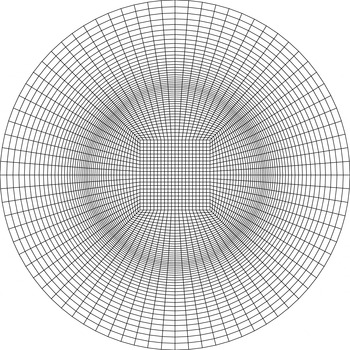
The spatially discretized
 $r{-}{\it\theta}$
plane used for quasi-two-dimensional numerical simulations with macro elements shown.

2.2.2. Quasi-two-dimensional model
An efficient alternative to the full non-axisymmetric simulations is the employment of a two-dimensional model to compute the flow on a horizontal plane (e.g. van de Konijnenberg et al.
Reference van de Konijnenberg, Nielsen, Juul Rasmussen and Stenum1999; Bergeron et al.
Reference Bergeron, Coutsias, Lynov and Nielsen2000; Früh & Nielsen Reference Früh and Nielsen2003; Schaeffer & Cardin Reference Schaeffer and Cardin2005). The model integrates out the vertical direction, for which the frictional effects are instead modelled by external forcing terms. Thus, the model only simulates the flow in the
 $r$
and
 ${\it\theta}$
dimensions. With the additional forcing term, (2.5a
) becomes
 $$\begin{eqnarray}{\displaystyle \frac{\partial \boldsymbol{u}_{\bot }}{\partial t}}+(\boldsymbol{u}_{\bot }\boldsymbol{\cdot }\boldsymbol{{\rm\nabla}}_{\bot })\boldsymbol{u}_{\bot }=-\boldsymbol{{\rm\nabla}}_{\bot }P_{\bot }+{\displaystyle \frac{\mathit{Ek}\,A^{2}}{1-A\mathit{Ro}}}{{\rm\nabla}_{\bot }}^{2}\boldsymbol{u}_{\bot }+{\displaystyle \frac{2\sqrt{Ek}}{1-A\mathit{Ro}}}(\boldsymbol{u}_{b}-\boldsymbol{u}_{\bot }),\end{eqnarray}$$
where
 $\boldsymbol{u}_{b}$
expresses the motion of the horizontal boundaries and the subscript
 $\bot$
represents the projection onto the quasi-two-dimensional plane. The last term on the right-hand side of the equation is a forcing term describing the Ekman friction from the boundary layers on the horizontal boundaries. This model is known as the quasi-two-dimensional model.
The
 $r{-}{\it\theta}$
domain is mapped onto a two-dimensional Cartesian grid as shown in figure 3. The discontinuous azimuthal velocity forcing across the radius at the disk–tank interface in the traditional boundary conditions described in § 2.2.2 was found to be unsuitable with the current discretized domain. This is because the discontinuity in the forcing exacerbates the four-fold symmetry of the mesh, which is composed of quadrilateral elements. This results in artificial energy being fed into the harmonics of the wavenumber 2 structure, heavily biasing even-wavenumber structures. This bias does not exist in the three-dimensional solutions as the three-dimensional domain retains its azimuthal homogeneity via the spectral-element–Fourier technique used for discretization in the azimuthal direction (§ 2.2.1). To circumvent this issue, a smoothing to the forcing is applied through the use of a hyperbolic tangent function over the transition zone. Hence, the forcing condition for the quasi-two-dimensional model is given by
 $$\begin{eqnarray}\boldsymbol{u}_{b}={\displaystyle \frac{{\it\Omega}r+{\displaystyle \frac{r}{2}}\left[1-\tanh \left({\displaystyle \frac{r-R_{d}}{{\it\delta}}}\right)\right]{\it\omega}}{{\it\Omega}R_{d}}},\end{eqnarray}$$
for all
 $r$
, where
 ${\it\delta}$
represents the thickness of the
 $\mathit{Ek}^{1/4}$
Stewartson layer (
 ${\it\delta}=(\mathit{Ek}/4)^{1/4}H$
). An advantage in using a hyperbolic tangent profile is that the derivative of any order is continuous (Bergeron et al.
Reference Bergeron, Coutsias, Lynov and Nielsen2000). This exact type of smoothing has been applied previously by van de Konijnenberg et al. (Reference van de Konijnenberg, Nielsen, Juul Rasmussen and Stenum1999), Bergeron et al. (Reference Bergeron, Coutsias, Lynov and Nielsen2000) and Früh & Nielsen (Reference Früh and Nielsen2003). An initial condition corresponding to a flow described by
 $\boldsymbol{u}_{b}$
is prescribed.
2.3. Stuart–Landau model
A Stuart–Landau model is used to investigate the weakly nonlinear dynamics of a complex oscillator in the vicinity of a bifurcation point. The Stuart–Landau equation describes the time variance of the complex amplitude
 ${\it\Lambda}$
of an unstable mode and can be used to establish the nature of non-axisymmetric transitions. The Stuart–Landau equation is defined as
 $$\begin{eqnarray}{\displaystyle \frac{\text{d}{\it\Lambda}}{\text{d}t}}=({\it\sigma}+\text{i}{\it\omega}){\it\Lambda}-l(1+\text{i}c)|{\it\Lambda}|^{2}{\it\Lambda}+\cdots \,,\end{eqnarray}$$
where
 ${\it\sigma}$
,
 ${\it\omega}$
,
 $l$
, and
 $c$
are all real-numbered coefficients. Here,
 ${\it\omega}$
is the angular oscillation frequency during the linear growth regime,
 ${\it\sigma}$
is the growth rate of a particular mode, and
 $c$
is a non-dimensional parameter known as the Landau constant. The quantity
 $l$
is dimensional and its sign can be used to categorize whether a transition is supercritical or subcritical. For supercritical bifurcations, the amplitude of the instability decreases to zero as the bifurcation parameter decreases towards the critical value. In contrast, subcritical bifurcations exhibit hysteresis near the transition which results in a flow condition expressing multiple stable states (e.g. bi-stability). The Stuart–Landau model has been used extensively in the investigations of bluff-body wake transitions and has been applied to stability analyses (Provansal, Mathis & Boyer Reference Provansal, Mathis and Boyer1987; Le Gal, Nadim & Thompson Reference Le Gal, Nadim and Thompson2001; Sheard, Thompson & Hourigan Reference Sheard, Thompson and Hourigan2004a
,Reference Sheard, Thompson and Hourigan
b
; Thompson & Le Gal Reference Thompson and Le Gal2004; Hussam, Thompson & Sheard Reference Hussam, Thompson and Sheard2011). However, this type of modelling has also been used for instabilities in weakly nonlinear rotating flow similar to those studied here (van de Konijnenberg et al.
Reference van de Konijnenberg, Nielsen, Juul Rasmussen and Stenum1999; Bergeron et al.
Reference Bergeron, Coutsias, Lynov and Nielsen2000).
It is proposed that the complex amplitude takes the form of
 $$\begin{eqnarray}{\it\Lambda}(t)={\it\gamma}(t)\text{e}^{\text{i}{\it\phi}(t)},\end{eqnarray}$$
where
 ${\it\gamma}$
is the real and non-negative amplitude of
 ${\it\Lambda}$
, and
 ${\it\phi}$
is its phase. Substituting this expression into (2.9) and splitting the Stuart–Landau equation into the real and imaginary parts yields
 $$\begin{eqnarray}{\displaystyle \frac{\text{d}\log ({\it\gamma})}{\text{d}t}}={\it\sigma}-l{\it\gamma}^{2}+\cdots \,,\end{eqnarray}$$
and
 $$\begin{eqnarray}{\displaystyle \frac{\text{d}{\it\phi}}{\text{d}t}}={\it\omega}-lc{\it\gamma}^{2}+\cdots \,.\end{eqnarray}$$
These equations respectively describe the change in amplitude and phase of the unstable mode over time. Equation (2.11) takes on a linear function of
 ${\it\gamma}^{2}$
which is directly related to
 $|{\it\Lambda}|$
. Therefore, it is possible to apply this Stuart–Landau model to numerical results that measure
 $|{\it\Lambda}|$
. In this study,
 $|{\it\Lambda}|$
is taken to be the energy within each mode such that the amplitude is computed from
 $$\begin{eqnarray}|{\it\Lambda}_{k}|=\left[\text{}\int \text{}_{V}\boldsymbol{u}_{k}^{2}\,\text{d}V\right]^{1/2},\end{eqnarray}$$
where
 $k$
denotes the azimuthal wavenumber and
 $V$
is the volume of the computational domain.
The values of
 ${\it\sigma}$
and
 $l$
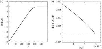
are determined by the vertical axis intercept and the gradient of a
 $\text{d}\log |{\it\Lambda}|/\text{d}t$
against
 $|{\it\Lambda}|^{2}$
plot, respectively. This is valid for times where
 $|{\it\Lambda}|$
is sufficiently small. Therefore,
 $l$
is determined close to the vertical axis. Assuming that the amplitude of the mode is initially small and saturates at a future time, the plot should demonstrate an initial point starting on the vertical axis with an end point on the horizontal axis. A positive slope (negative
 $l$
) at the vertical axis indicates that the transition is subcritical, whereas a negative slope (positive
 $l$
) indicates a supercritical transition.
3. Results: non-axisymmetric flow
The threshold of instability for the
 $A=2/3$
configuration has been previously determined as
 $\mathit{Ro}_{c}=18.1(\pm 0.8)\mathit{Ek}^{0.767\pm 0.006}$
(Vo et al.
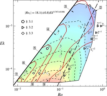
Reference Vo, Montabone and Sheard2014, Reference Vo, Montabone and Sheard2015). Figure 4 is a contour map of the most unstable wavenumber associated with the mode I instability as a function of
 $\mathit{Ro}$
and
 $\mathit{Ek}$
. The overlaid symbols and corresponding numbers represent the nonlinear unstable saturated modes obtained throughout this study. The figure summarizes the primary results of this paper. The thick dashed line represents the onset of symmetry-broken flow about the horizontal mid-plane, defined by
 $\mathit{Re}_{\mathit{Ek}}=26.7$
. The parameter
 $\mathit{Re}_{\mathit{Ek}}$
is the Reynolds number based on an Ekman thickness length scale, such that
 $\mathit{Re}_{\mathit{Ek}}=2\mathit{Ro}/\mathit{Ek}^{1/2}$
. It should be noted that there exists a transitional regime (
 $26.7\leqslant \mathit{Re}_{\mathit{Ek}}\leqslant 56.4$
) that encompasses both reflectively symmetric and symmetry-broken flows (Vo et al.
Reference Vo, Montabone and Sheard2015).
A regime diagram of the preferred linear wavenumber in the positive
 $\mathit{Ro}{-}\mathit{Ek}$
parameter space. The thick solid line represents the threshold of instability defined by
 $\mathit{Ro}_{c}=18.1(\pm 0.8)\mathit{Ek}^{0.767\pm 0.006}$
. The numerical labels marked around the perimeter of the contour map represent the unstable linear wavenumber associated with the mode I instability. The arrows indicate flow conditions (enclosed by short-dashed lines) that are dominated by the corresponding wavenumber. The long-dashed line represents
 $\mathit{Re}_{\mathit{Ek}}=26.7$
, below which the underlying axisymmetric solutions preserve reflective symmetry about the mid-plane. A transitional regime exists in the range
 $26.7\leqslant \mathit{Re}_{\mathit{Ek}}\leqslant 56.4$
, where both reflectively symmetric and symmetry-broken flow are exhibited. The overlaid symbols and corresponding numbers represent the nonlinear unstable saturated modes obtained using three-dimensional direct numerical simulation. A label of integer
 $X$
denotes a flow which is dominated by wavenumber
 $X$
, with the second dominant Fourier mode being a harmonic of
 $X$
. Labels
 $X^{Y}$
denote flows which are dominated by wavenumber
 $X$
, with the second dominant mode being
 $Y$
which is not a harmonic of
 $X$
. Subscripts ‘
 $c$
’, ‘
 $p$
’ and ‘
 $i$
’ denote flows which respectively demonstrate chaotic, periodic and irregular temporal behaviour (steady-state otherwise). Flows investigated in §§ 3.1–3.3 are represented by pentagons (⬠), triangles (▹) and diamonds (♢), respectively. Points marked by a circle (○) are additional computed cases that are not described in detail in this paper. The thin solid lines (red online) are included for guidance, segregating the saturated nonlinear states.

With guidance from the linear stability analysis results in figure 4, three-dimensional direct numerical simulations have been performed at numerous flow conditions throughout the positive-
 $\mathit{Ro}$
parameter space to demonstrate the three-dimensional behaviour that manifests at parameters where the axisymmetric base flows are dominated by either the mode I or mode II instability modes. The selected flow conditions also serve to demonstrate nonlinear mode evolution, interactions, and the time dependence of the saturated states. It is expected that nonlinear effects become more pronounced when flow conditions are forced well beyond the onset of instability (Früh & Read Reference Früh and Read1999; Früh & Nielsen Reference Früh and Nielsen2003; Lopez & Marques Reference Lopez and Marques2010). This expectation stems primarily from the differences in the preferential wavenumber between the experimental observations (Früh & Read Reference Früh and Read1999) and numerical linear stability analysis (Vo et al.
Reference Vo, Montabone and Sheard2014, Reference Vo, Montabone and Sheard2015), and the differences in the developed flows (e.g. steady-state, period-doubled and highly irregular flows). Thus, the results of the full three-dimensional simulations have been separated into three parts: § 3.1 explores a flow case near the stability threshold which serves as a reference case throughout the paper, and § 3.2 investigates flows that are well beyond the onset of instability. Flow conditions well beyond the instability onset are achieved by either increasing
 $\mathit{Ro}$
or decreasing
 $\mathit{Ek}$
, or a variation of both while keeping
 $\mathit{Re}_{i}$
constant. In § 3.3 we present the sensitivity results of axisymmetric and non-axisymmetric initial solutions and a bifurcation analysis. The last section (§ 3.4) corresponds to the non-axisymmetric structures produced via quasi-two-dimensional modelling, and comparisons are drawn with the full three-dimensional results.
3.1. In the vicinity of instability onset
A flow at a moderate Ekman number and a small Rossby number characterized by
 $(\mathit{Ro},\mathit{Ek})=(0.05,3\times 10^{-4})$
is investigated. For this particular
 $\mathit{Ek}$
, linear stability analysis predicts a critical Rossby number of
 $\mathit{Ro}_{c}=0.036$
. Moreover, the internal Reynolds number is given by
 $\mathit{Re}_{i}=31~(\mathit{Re}_{i,c}\approx 22.4)$
. Hence, this condition is near the onset of linear instability and will be taken as the reference flow condition used for comparison throughout this paper.
For
 $\mathit{Ro}=0.05$
and
 $\mathit{Ek}=3\times 10^{-4}$
, the most unstable azimuthal wavenumber is predicted to be
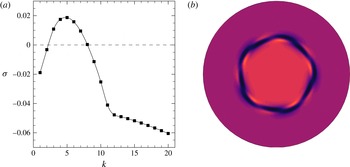
 $k=5$
according to linear stability analysis. The linear growth rates as a function of wavenumber and the axial vorticity contours constructed from the dominant eigenmode from the stability analysis for
 $k=5$
are illustrated in figure 5. The axial vorticity contours are only a depiction of the linear instabilities which have been arbitrarily amplified to finite amplitudes. Since
 $k=5$
is associated with the mode I waveband, the structure of the instability is reflectively symmetric about the mid-depth. Thus, the structure has a pentagonal appearance that extends vertically throughout the interior of the tank.
(a) The growth rates for a range of wavenumbers obtained through linear stability analysis for a flow condition of
 $\mathit{Ro}=0.05$
and
 $\mathit{Ek}=3\times 10^{-4}$
. The dashed line represents neutral stability, where points above and below symbolize unstable and stable wavenumbers, respectively. (b) Contours of axial velocity on the horizontal mid-plane (
 $z/H=0.5$
) for a velocity field constructed by superposing the axisymmetric basic flow with the dominant wavenumber 5 eigenmode scaled arbitrarily for visualization purposes. Contours of axial vorticity are plotted, with equi-spaced contour levels in the range
 $2\overline{{\it\Omega}}\pm 10{\it\omega}$
. Dark and light flooded contours represent low and high vorticity values, respectively. The orientation is such that a positive
 $\mathit{Ro}$
causes the central region to rotate anticlockwise faster than the outer region.

The same flow condition is computed using three-dimensional direct numerical simulation, initialized from the steady-state axisymmetric base flow solution seeded with white noise. The three-dimensional simulation employs 24 Fourier modes. Simulations using different numbers of Fourier modes have been computed to ensure that the azimuthal spatial resolution is sufficient to capture the correct asymptotic azimuthal wavenumber state of the flow. Implementing additional Fourier modes demonstrated no changes to the observed structure as larger wavenumbers were effectively harmonics of the developing flow exhibiting lower energies. Typically, increasing
 $\mathit{Re}_{i}$
requires additional Fourier modes to accurately capture the small-scale structures in those flows. The purpose of the white noise is to seed all of the non-zero azimuthal Fourier modes with energy at a level higher than machine error but significantly below nonlinear amplitudes. This accelerates the development of any instabilities in the flow in what are sometimes extremely time-consuming simulations. In the linear regime at long times, wavenumbers that are unstable will increase in energy over time while stable wavenumbers will lose energy. However, it is also possible that non-modal transient effects may briefly amplify a linearly stable Fourier mode when nonlinear effects are considered (Blackburn, Barkley & Sherwin Reference Blackburn, Barkley and Sherwin2008).
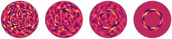
A time sequence of mode evolution from the initial white noise seeding is shown in figure 6 with contours of axial vorticity plotted on the horizontal mid-plane of the three-dimensional domain. The energies in the non-zero wavenumber structures are very small compared to the energy contained in the base flow during the initial developments, and would be invisible in a vorticity plot for the full flow field. Hence the fundamental (axisymmetric, zero-wavenumber) mode has been removed from the plotted fields, isolating the three-dimensional disturbance. As expected, the flow exhibits a chaotic appearance at early times, since noise is distributed randomly across all Fourier modes in the simulation. As the flow evolves, the dominant instability emerges, developing into a sinusoidal structure concentrated at a radial position consistent with the disk edge. The eventual instability forms a wavenumber 5 structure which is seen at
 $t=100$
. This is in agreement with the prediction from linear stability analysis. Since the instability adopts a sinusoidal form, a pairing of positive and negative vorticity represents a single wavelength of the disturbance. Hence, the frame at
 $t=100$
illustrates two disturbance rings representative of a wavenumber 5 structure.
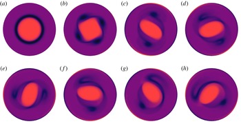
Evolution of a three-dimensional white-noise disturbance seeded onto an axisymmetric base flow with
 $\mathit{Ro}=0.05$
and
 $\mathit{Ek}=3\times 10^{-4}$
, which develops into a wavenumber 5 structure. The fundamental (axisymmetric) Fourier mode has been removed to isolate the disturbance field in these visualizations, and the flow is depicted on a horizontal plane at mid-depth. From left to right, the snapshots of axial vorticity are taken at
 $t=10$
, 20, 30 and 100. Equi-spaced contour levels are plotted in the range
 $\pm (|{\it\omega}_{z,min}|+|{\it\omega}_{z,max}|)/2$
. Dark and light flooded contours represent negative and positive values, respectively.

For three-dimensional flows that involve modal interactions, measurements of modal parameters are typically used as an indicator in demonstrating the most dominant mode in time. Examples of modal parameters include the kinetic energy (e.g. Henderson Reference Henderson1997; Lopez & Marques Reference Lopez and Marques2011), the amplitude (e.g. Sheard et al.
Reference Sheard, Thompson and Hourigan2004a
; Carmo, Meneghini & Sherwin Reference Carmo, Meneghini and Sherwin2010) and the enstrophy (e.g. Bergeron et al.
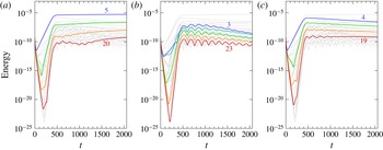
Reference Bergeron, Coutsias, Lynov and Nielsen2000; Früh & Nielsen Reference Früh and Nielsen2003) in each Fourier mode. Here, the kinetic energy measure as described by (2.13) is adopted. The energy contained in each non-zero azimuthal wavenumber over time for
 $\mathit{Ro}=0.05$
and
 $\mathit{Ek}=3\times 10^{-4}$
is displayed in figure 7(a). The zeroth wavenumber is omitted because changes in the energy of the axisymmetric mode are small in comparison to its absolute value. Indeed, the zeroth wavenumber contains the highest energy in the flow due to the large azimuthal velocities arising from the base rotation. Initially there is a rapid energy decrease due to the decay of the white noise belonging to stable wavenumbers. Following this, unstable wavenumbers are seen to gain energy at an exponential rate in the linear regime (
 $t\lesssim 450$
). As the modes grow in amplitude, nonlinear effects become significant and inhibit the exponential growth, leading to a saturated
 $k=5$
flow. Unchanging energy in the dominant wavenumber indicates that the unstable flow structure does not deform in time and drifts steadily about the axis of rotation.
Energy time series of the first 23 non-zero azimuthal wavenumbers for a flow condition of
 $\mathit{Ro}=0.05$
and
 $\mathit{Ek}=3\times 10^{-4}$
. (a) The bold lines represent the energies in the dominant wavenumber and its harmonics (
 $k=5,10,15,\dots \,$
). The bold lines in (b) represent the energies in wavenumbers
 $k=3,8,13,\dots \,$
, while the bold lines in (c) represent the energies in wavenumbers
 $k=4,9,14,\dots \,$
.

Harmonics of the dominant wavenumber (
 $k=10,15,20$
) are also seen to plateau after sufficient time in figure 7(a). Non-harmonic wavenumbers are seen to decay at varying rates with each demonstrating particular oscillations in their energy profiles. The oscillations are shared by groups of wavenumbers, such that a wavenumber belonging to a particular group illustrates oscillations in energy over time that are synchronized with the other wavenumbers belonging to the same group. For example, wavenumbers 3, 8, 13, 18 and 23 all demonstrate the same energy frequencies over time, as is seen in figure 7(b). Similarly, wavenumbers 4, 9, 14 and 19 illustrate similar oscillations amongst each other in figure 7(c). Thus, wavenumbers
 $k+k_{peak}n$
share similar oscillations in their energy over time, where
 $k_{peak}$
represents the dominant wavenumber at a particular time,
 $n$
is an integer (
 $n\geqslant 0$
) and
 $k$
is an integer azimuthal wavenumber (
 $1\leqslant k\leqslant k_{peak}$
). This relationship can be explained by the most dominant wavenumber imposing its symmetry onto all other wavenumber structures. This trend is also evident in the enstrophy time series provided by Früh & Nielsen (Reference Früh and Nielsen2003). The hierarchy of these wavenumbers in terms of the energy is typically described by the lowest wavenumber containing the highest energy which then cascades down to higher-wavenumber structures.
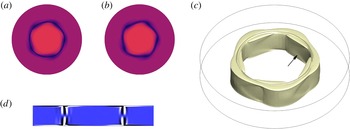
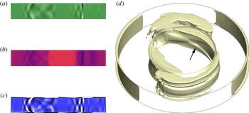
The contours of axial vorticity display a pentagon-shaped interior of high vorticity that is bordered by a ring of lower vorticity on the horizontal plane at saturation of the instability mode. This is shown in figure 8(a,b) at two different heights,
 $z/H=0.1$
and
 $z/H=0.5$
. From a top-down view, the structure drifts anticlockwise while the wave oscillates about
 $r=1$
and extends the entire depth of the tank with very little variability. The flow maintains a reflective symmetry about the horizontal mid-plane as demonstrated in the contours of azimuthal vorticity shown in figure 8(c), which is consistent with the underlying axisymmetric base flow solution. This nonlinear flow structure is very similar in appearance to that predicted by linear stability analysis (figure 5
b) and the energy time series does not demonstrate a vacillation from the linear to nonlinear regime (figure 7
a). A three-dimensional view of the nonlinear wavenumber 5 configuration is illustrated in figure 8(d) via an iso-surface of axial vorticity. The appearance of the distinct circular impression at the top of the iso-surface at
 $r=1$
is associated with the discontinuous boundary conditions imposed across the disk–tank interface. Thus, the expectation that nonlinear effects would have little effect in the vicinity of the stability threshold is supported.
(a,b) Contours of axial vorticity at two different heights of (a)
 $z/H=0.1$
and (b)
 $z/H=0.5$
for a flow condition of
 $\mathit{Ro}=0.05$
and
 $\mathit{Ek}=3\times 10^{-4}$
. These snapshots are taken at
 $t=910$
where the dominant mode has reached saturation. The flow is reflectively symmetric about
 $z/H=0.5$
. Contour levels are as in figure 5. (c) Contours of azimuthal vorticity displayed on the entire
 $r{-}z$
plane with levels plotted in the range
 ${\it\omega}_{{\it\theta}}=\pm 0.01|{\it\omega}_{{\it\theta},max}|$
, where dark and light flooded contours represent low and high values, respectively. (d) An isometric view of an iso-surface of axial vorticity
 ${\it\omega}_{z}=1.96$
representative of the saturated flow state at
 $t=2060$
. The arrow indicates the chevron-type patterns identified in the flow.

The features exhibited at
 $\mathit{Ro}=0.05$
and
 $\mathit{Ek}=3\times 10^{-4}$
, which is close to the instability threshold, were also observed in computations of other parameters combinations just beyond the onset of linear instability (refer to figure 4). The next section examines flow conditions further beyond the instability onset.
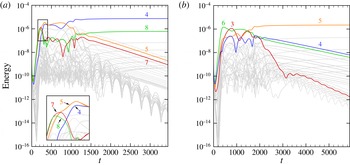
(a) Time series of the modal energies for a flow condition of
 $\mathit{Ro}=0.17$
and
 $\mathit{Ek}=2.5\times 10^{-4}$
. Energies of the first 39 non-zero modes are shown. Azimuthal wavenumbers 1, 2 and 5 are shown by bold lines. (b) Time evolution of axial vorticity of the three-dimensional flow. Time increases from left to right and continues in the bottom row. The times are given by
 $t=5,30,35,40,45,50,145$
and 1175, respectively. The three-dimensional simulation is initiated with the axisymmetric solution seeded with white noise. Contour levels are as in figure 5.

3.2. Flow conditions further beyond the instability onset
Flow conditions well beyond the onset of instability obtained by increasing the internal Reynolds number are described in this section. It is anticipated, in part due to the difference between experimental observations (Früh & Read Reference Früh and Read1999) and the dominant wavenumbers predicted from linear stability analysis (Vo et al.
Reference Vo, Montabone and Sheard2014, Reference Vo, Montabone and Sheard2015), that nonlinear effects will be significant in this region of the
 $\mathit{Ro}{-}\mathit{Ek}$
parameter space, producing a deviation from the linear predictions. The nonlinear effects are expected to primarily encourage the interaction and coalescence between vortices, which will in turn result in a smaller wavenumber structure. The increase in the internal Reynolds number is achieved by either increasing the Rossby number or decreasing the Ekman number, both of which are described separately in the following sections. A final section concludes our examination of flows well beyond the instability onset by investigating a constant high-
 $\mathit{Re}_{i}$
value at numerous
 $\mathit{Ro}$
and
 $\mathit{Ek}$
combinations.
3.2.1. Increasing the Rossby number
We now examine the case of a flow characterized by a Rossby number larger than that of the reference case, but having similar Ekman number. This case has
 $\mathit{Ro}=0.17$
,
 $\mathit{Ek}=2.5\times 10^{-4}$
, and a corresponding internal Reynolds number
 $\mathit{Re}_{i}=121$
, which is well beyond the critical value of
 $\mathit{Re}_{i,c}\approx 22.4$
. Linear stability analysis predicts a wavenumber 5 configuration to be the most unstable structure at this flow condition (figure 4), which has an eigenmode structure similar to that shown in figure 5(b).
This three-dimensional flow case has been computed using 40 azimuthal Fourier modes, as greater spatial resolution is required to capture time-dependent disturbances in the shear layer. This case was also computed using 24 Fourier modes, which described a very similar saturated solution to the case computed using 40 Fourier modes. The energy time series of the non-zero wavenumbers is shown in figure 9(a). Again, the flow is initialized with the axisymmetric base flow solution perturbed by white noise. A wavenumber 5 structure arises during the initial stages of the flow. However, the dominance of the
 $k=5$
structure is short-lived as the energy in wavenumber 2 becomes larger in comparison at approximately
 $t=80$
. Subsequently, the energy in
 $k=2$
and its harmonics plateaus over time while the energies of the odd wavenumbers decay. At
 $t\simeq 200$
the energies of the odd wavenumbers switch to an exponential growth behaviour, extracting energy from the fundamental mode, and eventually saturate at
 $t\approx 800$
with comparable amplitudes to the even wavenumbers. Eventually, the flow saturates to a state which is dominated by
 $k=2$
distorted by a wavenumber 1 structure (marked as ‘
 $2^{+1}$
’ in figure 4). The comparable energies in wavenumbers 1 and 2 causes both wavenumbers to impose their symmetries on weaker higher-wavenumber structures and therefore the similarity in energy oscillations typically exhibited by the group of
 $k+k_{peak}n$
wavenumbers is no longer valid.
The flow development represented through axial vorticity contours at mid-depth is illustrated in figure 9(b). A flow indistinguishable from the axisymmetric base flow solution is observed in the first frame at
 $t=5$
. A non-axisymmetric structure begins to evolve around the disk periphery at
 $r=1$
as the energies in the dominant wavenumbers increase in amplitude. At
 $t=35$
, four vortices are seen to form on one half of the initially axisymmetric shear layer. As time evolves, the vortices grow larger in size and the remaining shear layer also begins to roll up. Eventually, six vortices are observed at
 $t=45$
that are arranged irregularly, with the two vortices at the bottom of the frame being clustered close together. This pair of vortices coalesces at a future time and the structure adopts a pentagonal configuration. This initial process is reflected in the energy time series shown in figure 9(a). That is, the
 $k=5$
structure is dominant during the exponential growth regime. It is noted that the wavenumber 5 structure at
 $t=50$
is an asymmetric pentagon, and that a regular pentagon was not observable at other time steps. This is due to the time dependence of the flow as the energies in many of the wavenumbers are still varying at comparable amplitude.
At future times, the nonlinear effects cause the vortices to coalesce, resulting in a dipolar structure at
 $t=145$
. The two vortices exhibit low vorticity and encircle an oval-shaped interior of higher vorticity. This eventually becomes distorted as one of the vortices breaks and deforms into a strand as seen at
 $t=1175$
. The transition from a symmetric dipole state to a distorted state is reflected in the energy time series whereby increases in the wavenumber 1 structure are observed until it becomes comparable to the energy contained in the wavenumber 2 structure. Again, the constant energies displayed by the dominant modes indicate that the structure is unchanging and drifts steadily about the axis of rotation. A similar asymmetric dipole structure was obtained numerically by Früh & Nielsen (Reference Früh and Nielsen2003) in the same system using a quasi-two-dimensional model. A similar structure was also captured experimentally by van de Konijnenberg et al. (Reference van de Konijnenberg, Nielsen, Juul Rasmussen and Stenum1999). However, they observed a smooth vortex on one side and an unstable structure on the opposite side where small vortices continuously formed and dissipated. The differences in flow conditions and apparatus in that study may be reasons why the time-dependence is not seen here.
Distinct alternating weak and strong bands of axial vorticity are observable in the vortices and the interior region at
 $t=145$
and
 $t=1175$
. Examination of the discretized domain underlying the axial vorticity contours demonstrated that these waves are significantly larger than the radial and azimuthal grid spacings. Thus, these structures are a physical feature of the flow which we suspect to be inertial waves. Inertial waves arise in rotating flows due to the Coriolis force acting as a restoring force and exhibit frequencies in the range
 $0<{\it\omega}_{d}/\overline{{\it\Omega}}<2$
, where
 ${\it\omega}_{d}$
and
 $\overline{{\it\Omega}}$
are angular velocities of the drifting polygonal structure and the background flow, respectively (e.g. see Lopez & Marques Reference Lopez and Marques2011, Reference Lopez and Marques2014, and references therein). In this system, the waves are stationary with respect to the rotating polygonal structure and satisfy
 ${\it\omega}_{d}/\overline{{\it\Omega}}<2$
. These waves appear to originate from the disk–tank interface where the Stewartson and Ekman layers interact. This interaction may be related to the generation of these waves – a feature common with other configurations involving Ekman and Stewartson layers (e.g. Hart & Kittelman Reference Hart and Kittelman1996; Sauret et al.
Reference Sauret, Cébron, Le Bars and Le Dizès2012; Lopez & Marques Reference Lopez and Marques2014). Instabilities of the Ekman and Stewartson layers have been reported as the driving mechanism in rotating spherical shells (Noir, Jault & Cardin Reference Noir, Jault and Cardin2001; Calkins et al.
Reference Calkins, Noir, Eldredge and Aurnou2010) and differentially rotating configurations (Lopez & Marques Reference Lopez and Marques2010), respectively. It should be noted that visually similar wave patterns have been also observed in prior studies which have investigated spontaneous emergence of inertia–gravity waves from the interaction of two counter rotating vortices (e.g. Viúdez & Dritschel Reference Viúdez and Dritschel2006; Snyder et al.
Reference Snyder, Muraki, Plougonven and Zhang2007; Wang, Zhang & Snyder Reference Wang, Zhang and Snyder2009). A thorough review of inertia–gravity waves from atmospheric jets and fronts can be found in Plougonven & Zhang (Reference Plougonven and Zhang2014).
The same flow conditions simulated at a lower azimuthal resolution of 24 Fourier modes yielded a similar energy time series and similar vorticity and velocity contours. Thus, these small-scale wave patterns are not a numerical artefact. It is expected that these features would be very difficult to capture experimentally using laboratory techniques such as laser Doppler velocimetry and particle image velocimetry, since the azimuthal vorticity values are so much smaller than the values of axial vorticity in the flow. However, an altimetric imaging velocimetry technique has been able to successfully capture such structures (e.g. Afanasyev, Rhines & Lindahl Reference Afanasyev, Rhines and Lindahl2008). Despite the experimental limitation, the dipole captured here by direct numerical simulation is in agreement with the wavenumber range at these parameters reported from the experiments of Früh & Read (Reference Früh and Read1999): they reported wavenumbers 2–4 in the vicinity of
 $\mathit{Ro}=0.17$
and
 $\mathit{Ek}=2.5\times 10^{-4}$
.
Despite the complex patterns observed in the
 $r{-}{\it\theta}$
plane, the saturated flow still maintains reflective symmetry about the horizontal mid-plane. This symmetry is consistent with the axisymmetric solution at the same parameters (
 $\mathit{Re}_{\mathit{Ek}}=21.5$
, figure 4). Figure 10(a–c) illustrates contours of the axial velocity, axial vorticity and azimuthal vorticity on the vertical semi-plane of the tank (
 $r{-}z$
plane). All three contours are illustrated at the same arbitrary azimuthal angle and show reflective symmetry about the mid-depth. The axial velocity exhibits Ekman pumping at the disk–tank interface in addition to recirculation zones on either side. The recirculation zones are bounded by oblique waves which vary throughout the domain. This is in contrast to the reference flow case where the structures are not significantly inclined (see figure 8
c). These inclined structures can also be seen in the axial vorticity, and especially in the azimuthal vorticity, where low vorticity contours have been emphasized. Visualizations of the flow over time reveal that these inclined structures drift at the same rate as the primary polygonal structure (i.e. they are stationary relative to the rotating structure). In addition, the wave patterns can be seen in an iso-surface of axial vorticity as illustrated in figure 10(d). Closer inspection of the reference case flow also reveals chevron-type patterns in the iso-surface of axial vorticity (figure 8
c), though they are not as prominent. The weaker wave patterns observed in the reference case flow may be due to the lower Rossby number. Increases to the Rossby number drives a stronger axial jet flow in the Stewartson layers while decreasing the Ekman number produces thinner Stewartson layers, both of which increases the susceptibility of instability (Vo et al.
Reference Vo, Montabone and Sheard2014, Reference Vo, Montabone and Sheard2015) and hence the emergence of inertial waves (Lopez & Marques Reference Lopez and Marques2010). This result is evident throughout the parameter space explored in this paper.
Flow condition of
 $\mathit{Ro}=0.17$
and
 $\mathit{Ek}=2.5\times 10^{-4}$
at
 $t=1629$
. (a–c) Contours of (a) axial velocity, (b) axial vorticity and (c) azimuthal vorticity are displayed on the entire
 $r{-}z$
plane. Axial vorticity and azimuthal vorticity contour levels are as in figure 8 while axial velocity contour levels are plotted in the range
 $u_{z}=\pm 0.1|\mathit{Ro}|({\it\Omega}+{\it\omega})$
, where dark and light contour shading represent low and high values, respectively. (d) An isometric view of an axial vorticity iso-surface of
 ${\it\omega}_{z}=1.88$
is shown. The arrow indicates the chevron-type patterns identified in the flow.

The next section also investigates a flow condition that is well beyond the onset of instability, though achieved by decreasing the Ekman number of the reference flow case rather than by increasing the Rossby number.
3.2.2. Decreasing the Ekman number
The effect of decreasing the Ekman number to increase
 $\mathit{Re}_{i}$
is examined at flow conditions of
 $\mathit{Ro}=0.05$
and
 $\mathit{Ek}=8\times 10^{-5}$
. This reduction in Ekman number causes the investigated point to be at an internal Reynolds number of
 $\mathit{Re}_{i}=83.6$
, significantly beyond the instability threshold
 $\mathit{Re}_{i,c}\approx 22.4$
. Therefore, it is expected that, as in the previous section, the unstable wavenumber from the three-dimensional simulations will be different to the wavenumber predicted by linear stability analysis due to nonlinear effects. More specifically, the nonlinear state will adopt a lower azimuthal wavenumber than its linear prediction.
As indicated in the regime diagram (figure 4), the linear preferred wavenumber increases with decreasing Ekman number at small Rossby numbers. The predicted wavenumber here is 8, as compared to 5 for the reference case. Since the growth rates of the most unstable wavenumber is associated with the mode I instability, the eigenmode exhibits a central octagon exhibiting high values of vorticity with a thin ring of lower vorticity surrounding it.
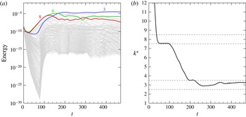
Here the three-dimensional flow has been resolved using 128 azimuthal Fourier modes. The energy time series of each non-zero wavenumber is shown in figure 11(a). The three-dimensional solution has been initialized with the axisymmetric base flow solution perturbed with white noise. It can be seen that the energies contained in the wavenumber 6 and 8 structures are initially the highest throughout the linear growth regime. The appearance of the wavenumber 6 structure in the linear regime rather than the dominant
 $k=8$
mode is explained by the small difference (less than 5 %) in their respective growth rates, and the possibility that the initial white-noise seeding may unevenly seed the unstable azimuthal wavenumbers. The competition between
 $k=6$
and
 $k=8$
structures weakens beyond
 $t\approx 100$
as nonlinear effects become significant. At this time, the energy in
 $k=8$
and subsequently
 $k=6$
begin to decrease, and the flow becomes dominated by a stable
 $k=3$
configuration by
 $t\approx 160$
. Unlike the
 $k=2^{+1}$
mode obtained earlier, the second dominant mode for this flow is a harmonic of the dominant wavenumber. Thus, an undisrupted triangular structure is expected to emerge in the three-dimensional flow.
Flow conditions of
 $\mathit{Ro}=0.05$
and
 $\mathit{Ek}=8\times 10^{-5}$
. Time series of (a) the energies contained in the first 127 azimuthal wavenumbers and (b) the averaged wavenumber weighted by energy. The dominant wavenumber transitions from
 $k=8$
to 6 to 3 over time represented by bold lines. The dashed lines enclosing
 $2.5\leqslant k^{\ast }<3.5$
and
 $7.5\leqslant k^{\ast }<8.5$
represent integer wavenumbers 3 and 8, respectively.

An alternative interpretation of the energy time series is achieved by considering the average wavenumber weighted by energy over time, as illustrated in figure 11(b) and calculated as
 $$\begin{eqnarray}k^{\ast }={\displaystyle \frac{\displaystyle \mathop{\sum }_{k=1}^{N}E_{k}k}{\displaystyle \mathop{\sum }_{k=1}^{N}E_{k}}},\end{eqnarray}$$
where
 $k$
is an integer azimuthal wavenumber,
 $N$
is the number of Fourier modes used in the simulation and
 $E_{k}$
is the energy contained in the
 $k$
th wavenumber. The energy associated with the base flow (
 $k=0$
) is omitted in calculating
 $k^{\ast }$
. The purpose of this quantity is to identify the dominant wavenumber that would be observed in the flow at a specific time, provided the amplitudes are not so small as to be swamped by the base flow. This parameter also helps to illustrate the wavenumber vacillation process when there are multiple wavenumbers competing with very large energies. The plot demonstrates a brief saturation of a wavenumber 8 structure (
 $7.5\leqslant k^{\ast }<8.5$
) in the time interval
 $35\lesssim t\lesssim 100$
. As the nonlinear effects become significant, the apparent wavenumber decreases towards
 $k^{\ast }=3~(2.5\leqslant k^{\ast }<3.5)$
and is sustained for
 $t\gtrsim 220$
. These changes in dominant wavenumber are consistent with the energies demonstrated in figure 11(a).
The three-dimensional wavenumber 3 structure achieved at saturation is represented in the contours of axial vorticity at two different depths, as shown in figure 12(a,b). The structure is composed of three concentrated regions of low vorticity migrating around the
 $r=1$
circumference. As described earlier, the contours near the horizontal boundary (
 $z/H=0.1$
) illustrate a circular ring of low vorticity attributed to the discontinuity at the disk–tank interface. The small-scale wavy structures described earlier (see figure 9
b) are evident in the interior and satellite vortices. As with the previous cases, this flow maintains its reflective symmetry about the horizontal mid-plane, as observed in the azimuthal vorticity contours in figure 12(c). An iso-surface of axial vorticity at
 $t=469$
is illustrated in figure 12(d). The iso-surface illustrates three vortices arranged in a triangle extending the entire depth of the tank. Additionally, distinct chevron-type features can be observed on the inner wall of the axial vorticity iso-surface.
Flow condition of
 $\mathit{Ro}=0.05$
and
 $\mathit{Ek}=8\times 10^{-5}$
at
 $t=469$
. (a,b) Contours of axial vorticity at two different heights of (a)
 $z/H=0.1$
and (b)
 $z/H=0.5$
. The flow is reflectively symmetric about the
 $z/H=0.5$
. Axial vorticity contour levels are as in figure 5. (c) Contours of azimuthal vorticity displayed on the entire
 $r{-}z$
plane with levels plotted as in figure 8. (d) An isometric view of an axial vorticity iso-surface of
 ${\it\omega}_{z}=1.96$
is shown. The arrow indicates the chevron-type patterns identified in the flow.

Increasing the flow conditions further beyond the instability onset by decreasing the Ekman number has shown similar characteristics to those exhibited by increasing the Rossby number. That is, the intensification of nonlinear effects encourages coalescence of vortices which yield wavenumbers that are smaller than the linear predictions. The flows presented so far in this paper have all demonstrated reflective symmetry about the horizontal mid-plane and steady saturated states. The next section details transitions between chaotic, steady and time-periodic flows observed at an even higher
 $\mathit{Re}_{i}$
.
3.2.3. High-
 $\mathit{Re}_{i}$
regime

Unsteady saturated and time-dependent flows have been reported in experimental and numerical studies at high-
 $\mathit{Re}_{i}$
conditions. Früh & Read (Reference Früh and Read1999) experimentally investigated a similar system and observed weak fluctuations, modulated oscillations, highly irregular flow, and period-doubled solutions in their positive-
 $\mathit{Ro}$
parameter space. Flows with weak fluctuations were discovered near the onset of instability at low
 $\mathit{Ek}$
while all other time-dependent flows were realized at high
 $\mathit{Re}_{i}$
values (both
 $\mathit{Ro}$
and
 $\mathit{Ek}$
being small or large). An extended experimental and numerical study conducted by Früh & Nielsen (Reference Früh and Nielsen2003) found time-dependent behaviour only for flows with three or fewer vortices for
 $\mathit{Re}\gtrsim 150$
(at constant
 $\mathit{Ek}=3\times 10^{-4}$
). A similar qualitative result was reported by van de Konijnenberg et al. (Reference van de Konijnenberg, Nielsen, Juul Rasmussen and Stenum1999), who found symmetric and steady flows for
 $k\geqslant 4$
and time-dependent flow for
 $k\leqslant 3$
in a parabolic bowl. Periodic deformations via slight oscillations of the triangular interior boundary for
 $k=3$
was seen while a periodic formation and decay of small vortices were obtained for
 $k=2$
. A decrease in wavenumber corresponded to an increase in Reynolds number. In their numerical simulations of the axisymmetric flows in this differential-disk system, Vo et al. (Reference Vo, Montabone and Sheard2014, Reference Vo, Montabone and Sheard2015) found no evidence of unsteady solutions throughout their computed Rossby and Ekman number ranges (
 $0.01\lesssim \mathit{Ro}\lesssim 0.6$
and
 $5\times 10^{-5}\lesssim \mathit{Ro}\lesssim 3\times 10^{-3}$
, respectively).
In unpublished experimental flow visualizations from particle tracking carried out in 1998, a typical travelling wavenumber 2 flow was revealed at
 $\mathit{Ro}=0.77$
and
 $\mathit{Ek}=1\times 10^{-3}$
. The apparatus used is described in Früh & Read (Reference Früh and Read1999). Increasing the Rossby number to
 $\mathit{Ro}=0.924$
while holding
 $\mathit{Ek}$
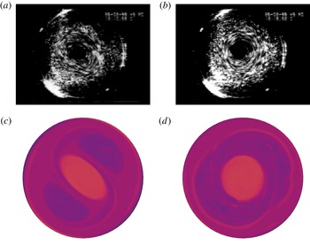
constant produced a flow which appears axisymmetric in the horizontal plane with an indication of a pair of toroidal Taylor-like vortices in the vertical plane. Images of the experimental flow visualization are shown in figure 13(a,b). To elucidate the flow structure and dynamics in this regime, this section investigates high-
 $\mathit{Re}_{i}$
flows based on the flow conditions investigated experimentally. Thereafter, the high-
 $\mathit{Re}_{i}$
condition is held constant while
 $\mathit{Ro}$
and
 $\mathit{Ek}$
are varied to examine whether or not the characteristics present at the high-
 $\mathit{Re}_{i}$
regime are dependent only on
 $\mathit{Re}_{i}$
, or if they are further a function of both
 $\mathit{Ro}$
and
 $\mathit{Ek}$
. Additionally, any transitions in the temporal properties of the flow will be described.
Flow conditions of (a,c)
 $\mathit{Ro}=0.77$
,
 $\mathit{Ek}=1\times 10^{-3}$
and (b,d)
 $\mathit{Ro}=0.924$
,
 $\mathit{Ek}=1\times 10^{-3}$
. Visual comparison between (a,b) experimental particle tracking and (c,d) the axial vorticity contours from a three-dimensional simulation. Axial vorticity contour levels as for figure 5.

The flow condition of
 $\mathit{Ro}=0.77$
and
 $\mathit{Ek}=1\times 10^{-3}~(\mathit{Re}_{i}=193)$
is considered first. An axisymmetric simulation of this flow condition demonstrates saturation towards a steady-state flow. The three-dimensional direct numerical simulation generates a wavenumber 2 structure first arising in the linear regime and remaining dominant during its nonlinear development. The energy in the wavenumber 1 structure increases gradually over time and eventually plateaus as the second most energetic non-zero wavenumber. Axial vorticity contours in the horizontal mid-plane illustrated in figure 13(c) exhibit excellent agreement with the experimental observations. Both the experimental visualization and three-dimensional simulation illustrate an elliptical vortex located at the centre of the tank with two vortices situated on opposite sides of the ellipse.
In contrast, significantly different dynamics are observed when the Rossby number is increased to
 $\mathit{Ro}=0.924~(\mathit{Re}_{i}=323)$
. For comparison against experimental visualization, a top-down view of the axial vorticity contours at mid-depth is provided in figure 13(d). The flow exposes a structure which is almost axisymmetric, especially in the central region, which is visually similar to that observed experimentally. A numerical simulation for the axisymmetric solution at this same flow condition was computed. At this higher Rossby number, the axisymmetric solution illustrates an unsteadiness in the axial jets supplied by Ekman pumping from the rapid disk rotation emanating from the disk–tank interfaces. The presence of stronger axial jets driven by faster spinning disks (larger
 $\mathit{Ro}$
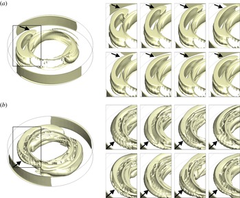
) causes an instability to develop as a breaking of the hyperbolic zone at the point where the jets meet. This unsteadiness in turn breaks the reflective symmetry about the horizontal mid-plane and the flow saturates to a perfect periodicity in time. This periodic flapping of the axial jets is not seen in the saturated three-dimensional flow, rather the axial jets become three-dimensional and fluctuate irregularly. This irregular fluctuation is shown in figure 14, which displays snapshots of an axial vorticity iso-surface over time. The iso-surface is chosen to conveniently highlight the breaking of the axial jets around the periphery of the disks.
Flow conditions of
 $\mathit{Ek}=1\times 10^{-3}$
and
 $\mathit{Ro}=0.924$
. (a) An oblique view of an iso-surface of axial vorticity in the three-dimensional flow. (b) Snapshots of axial vorticity over time shown through a close-up of the flow corresponding to the marked box in (a). The flow is shown in a stationary frame of reference relative to the rotating flow.

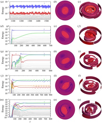
Flow conditions of a constant
 $\mathit{Re}_{i}=323$
at (a–c)
 $\mathit{Ek}=1\times 10^{-3},\mathit{Ro}=0.924$
, (d–f)
 $\mathit{Ek}=7\times 10^{-4},\mathit{Ro}=0.707$
, (g–i)
 $\mathit{Ek}=5\times 10^{-4},\mathit{Ro}=0.549$
, (j–l)
 $\mathit{Ek}=3\times 10^{-4},\mathit{Ro}=0.375$
, (m–o)
 $\mathit{Ek}=7\times 10^{-5},\mathit{Ro}=0.126$
. (a,d,g,j,m) Energy time series, (b,e,h,k,n) the axial vorticity contours illustrated in the
 $r{-}{\it\theta}$
mid-plane, (c,f,i,l,o) iso-surfaces of axial vorticity demonstrating the axial dependence of the flow structures. The axial vorticity plots are represented at times corresponding to the ending time of their respective energy time series.

Since the axisymmetric solution is periodic rather than steady state, the three-dimensional direct numerical simulation is not initialized with a prescribed base flow but rather begins with the axisymmetric boundary conditions (tank and disk rotation) and white noise. This is applicable to the remaining flows simulated in this section. The three-dimensional direct numerical simulation exhibits chaotic behaviour in the energies of all wavenumbers, as shown in figure 15(a). The saturated flow is described by a dominant wavenumber 2 structure with its first harmonic (
 $k=4$
) being the second dominant mode. The erratic oscillations in energy are caused by the irregular fluctuations in the axial vorticity strands stemming from the disk–tank interface when viewed in the
 $r{-}z$
plane. In this chaotic state, the reflective symmetry about the horizontal mid-plane is lost. Additional visualizations of the flow are also shown in figure 15(a) via contours and an iso-surface of axial vorticity to illustrate the depth dependence of the flow.
Other flows at
 $\mathit{Re}_{i}=323$
are investigated by decreasing both
 $\mathit{Ek}$
and
 $\mathit{Ro}$
. The energies of the non-zero wavenumbers, axial vorticity contours and iso-surfaces are illustrated in figure 15. As
 $\mathit{Ek}$
and
 $\mathit{Ro}$
decrease, the flow transitions from being chaotic at
 $\mathit{Ek}=1\times 10^{-3}$
to steady state at
 $5\times 10^{-4}\leqslant \mathit{Ek}\leqslant 7\times 10^{-4}$
. It should be noted that as the Ekman number is decreased, the energy in the wavenumber 1 structure increasingly becomes comparable to the wavenumber 2 mode while remaining the second dominant mode. This causes the initial dipole to rotate off-axis and broadens one of its vortices. Additionally, the central structure becomes thinner, loses symmetry and breaks apart with decreasing Ekman number. Despite the comparable energies in the leading modes, the energies maintain a plateau which demonstrates a steady-state solution. That is, the rigid instability structure drifts about the axis of rotation.
Further decreasing below
 $\mathit{Ek}=3\times 10^{-4}$
causes the wavenumber 1 structure to become dominant and compete with the wavenumber 2 structure. The vortex which was broadened due to the increase in energy in the wavenumber 1 structure eventually deforms into a strand of vorticity that no longer encloses a region of fluid (figure 15
d,e). The strand of vorticity folds back into itself partially and connects with the opposing vortex adopting an S-shaped appearance for the structure as a whole. In the case of
 $\mathit{Ek}=3\times 10^{-4}$
, the energies in the non-zero wavenumbers saturate to a clear periodic undulation over time. This undulation also exists at the lower
 $\mathit{Ek}=7\times 10^{-5}$
although it is weaker and not as obvious on a logarithmic scale and not perfectly periodic. That is, the temporal behaviour of the flow transitions from a periodic to an irregular state from
 $\mathit{Ek}=3\times 10^{-4}$
to
 $\mathit{Ek}=7\times 10^{-5}$
. The decrease in Ekman number also demonstrates more prominent waves in the flow.
At these smaller Ekman numbers, the unsteadiness is caused by a horizontal flapping of the axial vorticity strand. This periodic motion is illustrated in figure 16(a) over a time span coinciding with the period demonstrated in the energy oscillations for
 $\mathit{Ek}=3\times 10^{-4}$
. The strand of axial vorticity thickens as its tail curls towards the edge of the disk and becomes thinner as the tail kicks away from the disk. The opposing vortex does not deform significantly throughout this motion and the flow maintains a reflective symmetry about the horizontal mid-plane. A similar periodic motion is observed for
 $\mathit{Ek}=7\times 10^{-5}$
. However, the opposing vortex is much thinner and deformations are more prominent at this Ekman number as compared to
 $\mathit{Ek}=3\times 10^{-4}$
. In addition, there is a continuous formation and decay of vorticity at its periphery, which may be the cause of the imperfect undulations demonstrated in the energy time series. A similar feature was also observed by van de Konijnenberg et al. (Reference van de Konijnenberg, Nielsen, Juul Rasmussen and Stenum1999), although they reported the feature as being periodic and the vortices appeared coherent.
(a) Flow conditions of
 $\mathit{Ek}=3\times 10^{-4}$
and
 $\mathit{Ro}=0.375$
. Snapshots of axial vorticity over a time span corresponding to the period associated with the
 $k=1$
energy fluctuations. (b) Flow conditions of
 $\mathit{Ek}=1\times 10^{-3}$
and
 $\mathit{Ro}=0.924$
. Erratic changes in the flow are illustrated through snapshots of axial vorticity over two undulations in the dominant wavenumber 2 structure. The arrows in the insets indicate regions of interest as described in the text.

In stark contrast to the periodic and irregular flow observed at low
 $\mathit{Ek}$
, the fluctuations in energy for
 $\mathit{Ek}=1\times 10^{-3}$
are not caused by irregular wavering of the axial vorticity strand but rather erratic oscillations of the axial jets and continuous deformation of the axial vorticity patches situated at the periphery of the disk. The flow deformations over approximately two undulations of the energy in
 $k=2$
are illustrated in figure 16(b).
To our knowledge, this study is the first to report the wavering of the axial vorticity strand and recognize its association with periodic change in the energy of the dominant wavenumber. Bergeron et al. (Reference Bergeron, Coutsias, Lynov and Nielsen2000) were able to obtain flow states at large Reynolds number conditions which illustrated time-periodic behaviour when visualized with vorticity contours and through measurements of the global enstrophy. However, they did not provide a physical explanation as to why these flows exhibit this periodic behaviour. At least a single strand of axial vorticity can be seen in their figures 17 and 18, rather than a completely closed vortex, much like that shown in figure 16(a). Their time evolution snapshots appear to demonstrate a modulation of this axial vorticity strand, similar to the instability described here. The change they observe may be related to the wavering in the tail of the axial vorticity strand in addition to changing its size. This could be a possible explanation for their time-dependent behaviour. It must be noted that their time-periodic states were obtained with free-slip boundary conditions whereas no-slip boundary conditions are used in this study. They note that at very large Reynolds numbers, the no-slip boundary condition causes a continuous generation of vorticity erupting from the inner rod used to drive the rotation of the disks which leads to chaotic flow. Similar chaos was observed by Früh & Nielsen (Reference Früh and Nielsen2003), who reported that time-dependent flow may originate from a co-existence of global modes or from the generation of small vortices off the inner rod.
The pure and S-shaped dipole structures captured in these simulations resemble structures in Venus’s polar vortices. A dipole structure at the north pole of Venus was first mapped by the Pioneer Venus Orbiter in the 1970s in the middle atmosphere (Taylor et al. Reference Taylor, Diner, Elson, McCleese, Martonchik, Delderfield, Bradley, Schofield, Gille and Coffey1979, Reference Taylor, Beer, Chahine, Diner, Elson, Haskins, McCleese, Martonchik, Reichley, Bradley, Delderfield, Schofield, Farmer, Froidevaux, Leung, Coffey and Gille1980). The more recent European Space Agency’s Venus Express mission captured an S-shaped dipole structure at the south pole via the Visible and Infrared Thermal Imaging Spectrometer (Piccioni et al. Reference Piccioni, Drossart, Sanchez-Lavega, Hueso, Taylor, Wilson, Grassi, Zasova, Moriconi, Adriani, Lebonnois, Coradini, Bezard, Angrilli, Arnold, Baines, Bellucci, Benkhoff, Bibring, Blanco, Blecka, Carlson, Di Lellis, Encrenaz, Erard, Fonti, Formisano, Fouchet, Garcia, Haus, Helbert, Ignatiev, Irwin, Langevin, Lopez-Valverde, Luz, Marinangeli, Orofino, Rodin, Roos-Serote, Saggin, Stam, Titov, Visconti and Zambelli2007), though this is a thermal feature rather than a vorticity structure. The dynamics of Venus’s south polar vortex are very complex, with its internal structure constantly varying on a daily time scale (Luz et al. Reference Luz, Berry, Piccioni, Drossart, Politi, Wilson, Erard and Nuccilli2011; Garate-Lopez et al. Reference Garate-Lopez, Hueso, Sanchez-Lavega, Peralta, Piccioni and Drossart2013).
It should be noted that three-dimensional simulations have been performed in the present work at several flow conditions additional to those described in §§ 3.1–3.3 (these additional cases are included in figure 4). The simulations establish trends which describe saturated modes being equivalent to the wavenumber predicted by linear stability analysis for flows in the vicinity of the instability onset, and as the internal Reynolds number is increased either by increasing the Rossby number or decreasing the Ekman number, the structures of the stable flow state exhibit azimuthal structures that are different (lower wavenumber) from those predicted by linear stability analysis. The comparable energy in each azimuthal wavenumber structure exacerbates nonlinear effects, which causes unstable structures of varying wavenumbers to compete and interact.
In addition, it was also found (though not shown here), that wavenumbers associated with the mode II instability had little influence on the stability of the flow in the nonlinear regime. The energy in the mode II wavenumbers is observed to briefly dominate in the linear regime as for the linear stability analysis, but in the nonlinear regime their energy is seen to quickly decay. Thus, the mode II instability is not expected to dictate the structure of real flows. The next section investigates the sensitivity of a flow and the hysteretic nature of the primary instabilities present in these flows.
3.3. Flow sensitivity and bifurcation analysis
The sensitivity of the three-dimensional flow is investigated in this section via two different studies. The first considers initializing the steady-state axisymmetric base flows perturbed with various initial conditions at constant
 $\mathit{Ro}$
and
 $\mathit{Ek}$
to examine the variation of the stable azimuthal wavenumbers observed upon saturation. The second considers changing the Rossby number of a saturated three-dimensional flow to investigate hysteresis effects which have been observed experimentally (e.g. Früh & Read Reference Früh and Read1999). These cases are discussed separately in the following sections. Following this, a bifurcation analysis of the various linear instability modes determined through linear stability analysis is presented.
3.3.1. Perturbing the axisymmetric solution
The saturated three-dimensional flows observed in the previous sections were initialized from the evolved steady-state axisymmetric solution perturbed with white noise. Since many of the prior energy time series demonstrated a single stable azimuthal wavenumber of very large energy compared to the other wavenumbers, it is expected that different initial conditions of the same flow condition will achieve the same stable solution. In this section, the steady-state axisymmetric base flows are initially seeded with various unstable linear mode solutions, with and without white noise.
A flow characterized by
 $\mathit{Ro}=0.5$
and
 $\mathit{Ek}=3\times 10^{-3}$
is considered for investigation here. The large growth rates inherent in the high-
 $\mathit{Ro}$
and high-
 $\mathit{Ek}$
flow allows for shorter computation times in reaching a saturated solution. According to the linear stability analysis, the most unstable wavenumber is predicted to be
 $k=3$
. The growth rates of this flow and its linear instability structure are shown in figure 17(a) and its inset, respectively.
Flow condition of
 $\mathit{Ro}=0.5$
and
 $\mathit{Ek}=3\times 10^{-3}$
. (a) The growth rates for a range of wavenumbers obtained through linear stability analysis. The dashed line represents neutral stability, where points above and below symbolize unstable and stable wavenumbers, respectively. The inset shows representative axial vorticity contours of linear instabilities of finite amplitude superimposed onto its respective steady-state axisymmetric base flow shown at
 $z/H=0.5$
. Nonlinear effects have been neglected, and contour levels are as in figure 5. (b) Energies of the first 23 non-zero wavenumbers over time. The inset shows typical contours of axial vorticity at
 $z/H=0.5$
of a saturated flow regardless of the initial conditions provided they are axisymmetric. Equi-spaced contour levels are plotted in the range
 $2\overline{{\it\Omega}}\pm 5{\it\omega}$
.

A three-dimensional direct numerical simulation has been initialized with its steady-state axisymmetric base flow and white noise. The energies contained in each azimuthal wavenumber over time for the first 23 non-zero wavenumbers are shown in figure 17(b). The three-dimensional solution agrees with the linear prediction as the energy in the wavenumber 3 structure is dominant during the initial stages of the flow development. The structures of the linear and nonlinear wavenumber 3 structures are very similar in appearance. As nonlinear effects become apparent, the even wavenumbers slowly increase in energy over time and eventually surpass the wavenumber 3 structure, resulting in a dominant wavenumber 2 flow.
To see the effects of different initial conditions, the steady-state axisymmetric base flow was seeded with an instability mode of a single wavenumber. Eigenvectors for
 $k=2,3,4$
and
 $k=6$
were separately seeded into the initial steady-state axisymmetric base flow and the energies of the leading wavenumbers were monitored until the flow evolved into a saturated state. As the non-seeded flow indicated a wavenumber 2 structure at saturation (figure 17
b), it is expected that all seeded flows will ultimately produce the same wavenumber provided the axisymmetric flow is insensitive to initial conditions. For all eigenvector-seeded cases, the wavenumber 2 structure and its harmonics prevail and demonstrate saturated energy profiles similar to that obtained by the non-seeded case. For example, a wavenumber 3 seeded eigenvector illustrates a triangular structure at the initial state which evolves into a dipole structure at the final state due to nonlinear interactions as the energies in the odd wavenumbers decay. The axial vorticity contours of a typical nonlinear solution for the saturated wavenumber 2 at this flow condition is depicted in the inset of figure 17(b).
The sensitivity of axisymmetric flow solutions at other flow conditions has also been analysed. A lower limit of
 $\mathit{Ro}=0.1$
and
 $\mathit{Ek}=2\times 10^{-4}$
was considered for investigation as lesser forcing conditions require a longer time integration and greater computational resources to simulate the smaller growth rates and flow structures. The tested flow solutions have all shown the same insensitivity characteristics as
 $\mathit{Ro}=0.5$
and
 $\mathit{Ek}=3\times 10^{-3}$
(figure 17). This type of insensitivity has also been observed by Bergmann et al. (Reference Bergmann, Tophøj, Homan, Hersen, Andersen and Bohr2011), who studied a different type of rotating flow. In that study, the sensitivity of the flow was examined through the testing of various initial conditions involving a flow initialized from rest, initialized from manually disrupting a developed triangular structure and initialized with a high rotation rate such that the flow was axisymmetric. The resultant flow for all three cases exhibited a triangle, which suggests that the flow was insensitive to initial conditions.
3.3.2. Perturbing the non-axisymmetric solution
To further study the flow sensitivity, the effect of hysteresis was investigated by changing the forcing conditions of non-axisymmetric saturated flows. This change in forcing is to mimic, to an extent, experimental conditions which have experienced strong hysteresis and have shown dependence on the direction of the change of experimental conditions (e.g. Früh & Read Reference Früh and Read1999; van de Konijnenberg et al. Reference van de Konijnenberg, Nielsen, Juul Rasmussen and Stenum1999; Bergeron et al. Reference Bergeron, Coutsias, Lynov and Nielsen2000; Früh & Nielsen Reference Früh and Nielsen2003).
Two saturated flow conditions of
 $\mathit{Ro}=0.0325$
and
 $\mathit{Ro}=0.02375$
at
 $\mathit{Ek}=8\times 10^{-5}$
have been interchanged. The Rossby number is changed instantly from
 $\mathit{Ro}=0.0325$
to
 $0.02375$
and vice versa at an arbitrary time after a stable saturated flow has been reached. These flow conditions were chosen such that they belong in the lower parameter regime, in contrast to the previous section, to illustrate the lower growth rates and that the hysteresis effects can occur over a minor change in
 $\mathit{Ro}$
. Additionally, large
 $\mathit{Ek}$
conditions do not display a large variety of unstable wavenumbers and therefore are not suitable for this type of sensitivity study. The Rossby number was varied instead of the Ekman number because it demonstrated a rapid change in wavenumber over a small range. The energy time series of these saturated flow solutions are depicted in figure 18. Stable wavenumbers of
 $k=4$
and
 $k=5$
are exhibited in the saturated state for
 $\mathit{Ro}=0.0325$
and
 $\mathit{Ro}=0.02375$
, respectively, which differ from the linearly predicted state of
 $k=7$
for both flows (refer to figure 4).
The energy time series for
 $\mathit{Ek}=8\times 10^{-5}$
, for (a)
 $\mathit{Ro}=0.0325$
with the first 39 non-zero wavenumbers with an inset illustrating a close-up region of the competing modes just beyond the linear regime, and (b)
 $\mathit{Ro}=0.02375$
with the first 31 non-zero wavenumbers. Saturated stable states of
 $k=4$
and
 $k=5$
are obtained for each flow, respectively.

The non-axisymmetric solution of
 $\mathit{Ro}=0.0325$
and
 $\mathit{Ek}=8\times 10^{-5}$
at
 $t=2350$
is used as the initial condition. This time is marked by a vertical dashed line as shown in figure 19(a), and corresponds to a time where the dominant mode has saturated. The axial vorticity structure at this nominated time (
 $t=2350$
) and the final time (
 $t=3450$
) display no significant differences. At
 $t=2350$
, the flow is dominated by a wavenumber 4 structure with the energy in its harmonics saturating over time while all other wavenumbers are decaying. As the Rossby number is decreased to
 $\mathit{Ro}=0.02375$
, the energies in each azimuthal wavenumber drop gradually over a short time period. The energies in each wavenumber then demonstrate the same trends established before
 $t=2350$
. That is, a stable square configuration is observed and the harmonics of
 $k=4$
approach a plateau. The wavenumber 5 structure, which was determined to be most unstable mode for
 $\mathit{Ro}=0.02375$
(see figure 18
b), continues to decay. Thus, bi-stability is evident. The contours of axial vorticity at
 $z/H=0.5$
are illustrated in the inset of figure 19(a).
The Rossby number is changed from (a)
 $\mathit{Ro}=0.0325\rightarrow \mathit{Ro}=0.02375$
and (b)
 $\mathit{Ro}=0.02375\rightarrow \mathit{Ro}=0.0325$
with
 $\mathit{Ek}=8\times 10^{-5}$
. Energies of various non-zero wavenumbers over time with the change in
 $\mathit{Ro}$
occurring instantaneously at
 $t=2350$
and
 $t=3500$
, respectively, which have been marked by a vertical dashed line. The insets show the axial vorticity contours extracted at
 $z/H=0.5$
at
 $t=3750$
and
 $t=9150$
, respectively. Contour levels are as in figure 5.

The energy time series for the reverse case of increasing the Rossby number from
 $\mathit{Ro}=0.02375$
to
 $\mathit{Ro}=0.0325$
at
 $\mathit{Ek}=8\times 10^{-5}$
is shown in figure 19(b). The change in flow conditions is marked by a vertical dashed line at
 $t=3500$
. The increase in
 $\mathit{Ro}$
causes a sharp increase in energy for all of the azimuthal wavenumbers. The flow continues to sustain the wavenumber 5 structure over a long period of time with energies from
 $k=4$
gradually decreasing. At approximately
 $t=8000$
, the energies in
 $k=4$
increase and eventually become dominant at
 $t=8450$
. Thus, the stable configuration observed is the same as that obtained from initializing the flow from the steady-state axisymmetric base flow with a flow condition of
 $\mathit{Ro}=0.0325$
and
 $\mathit{Ek}=8\times 10^{-5}$
.
This pair of flow conditions has demonstrated that multiple stable saturated states may exist at a single flow condition, depending on how it is approached. This hysteretic behaviour is in agreement with the strong hysteresis observed in previous studies of similar shear layer systems (Früh & Read Reference Früh and Read1999; Bergeron et al. Reference Bergeron, Coutsias, Lynov and Nielsen2000; Hollerbach et al. Reference Hollerbach, Futterer, More and Egbers2004; Aguiar et al. Reference Aguiar, Read, Wordsworth, Salter and Hiro Yamazaki2010).
3.3.3. Bifurcation analysis
The hysteretic nature of the three different linear instability transitions, namely modes I, II and III (see Vo et al.
Reference Vo, Montabone and Sheard2014), has been investigated. The Stuart–Landau model (§ 2.3) has been applied to the most unstable linear wavenumber and its harmonics. The nonlinear behaviour is determined through the sign of the
 $l$
parameter. The restriction of simulating a particular wavelength and its harmonics is achieved numerically through a truncation of the azimuthal range of the domain to exactly fit the wavelength of interest. As a consequence of the axisymmetry of the domain, only the considered wavenumber and its harmonics are able to fit perfectly in the truncated domain. Each numerical study has been initiated with the axisymmetric base flow solution seeded with the most unstable eigenmode scaled to very small amplitudes.
The transitional behaviour of the mode I instability of
 $\mathit{Ro}=0.05$
and
 $\mathit{Ek}=3\times 10^{-4}$
is investigated. A plot of the growth rate against wavenumber is shown in figure 5(a), which illustrates the existence of only the mode I instability and is most unstable to a wavenumber 5 configuration. The mode transition is determined to be supercritical, which can be deduced from figure 20. Initially, the amplitude of the wavenumber 5 instability is small and grows exponentially in time until it plateaus at approximately
 $t=440$
. This exponential trend is representative of the linear regime, which is required to obtain an accurate gradient near the vertical axis in figure 20(b). The gradient at the vertical axis corresponds to the
 $l$
parameter in the Stuart–Landau equation. The negative slope (having
 $l=4.55\times 10^{-6}$
) indicates that the mode evolution is supercritical. The
 $\text{d}\log |{\it\Lambda}|/\text{d}t$
curve approaches the horizontal axis as the mode saturates. The intercept of the vertical axis, which represents the growth rate of the mode in the linear regime, has a value of 0.0187, identical to that predicted by linear stability analysis (see figure 5
a).
Flow conditions described by
 $\mathit{Ro}=0.05$
and
 $\mathit{Ek}=3\times 10^{-4}$
. (a) Amplitude of the most unstable isolated mode corresponding to wavenumber 5 against time. (b) The rate of change in amplitude over time against the square of the amplitude. A negative linear gradient at the vertical axis indicates that the transition is supercritical.

A range of other flow conditions that are dominated by the mode I instability have also been investigated. The same Stuart–Landau model consistently finds the transition of the mode I instability to be supercritical. This confirms and extends the experimentally determined supercritical behaviour detected for low-wavenumber instability by Früh & Read (Reference Früh and Read1999), van de Konijnenberg et al. (Reference van de Konijnenberg, Nielsen, Juul Rasmussen and Stenum1999) and Bergeron et al. (Reference Bergeron, Coutsias, Lynov and Nielsen2000). In addition, the Stuart–Landau model has been applied to a variety of flow conditions that encourage the growth of the mode II and III instability modes. The
 $l$
parameter has been determined to be positive in all flow cases, which suggests that the weakly nonlinear mode evolution behaviour in this type of rotating flow is supercritical.
3.4. Comparison with quasi-two-dimensional model results
The non-axisymmetric structures in these rotating flows are now investigated using a quasi-two-dimensional model to elicit the differences compared to the computationally expensive three-dimensional model. Unlike the previous three-dimensional simulations, the quasi-two-dimensional model computes the non-axisymmetric flow on a two-dimensional
 $r{-}{\it\theta}$
domain, and by definition there can be no depth dependence. In addition, the forcing conditions used here are smoothed (described in § 2.2.2), which are different to those employed in the three-dimensional direct numerical simulation (§ 2.2.1). Despite these differences, the flow conditions computed for the three-dimensional model are simulated here for the quasi-two-dimensional model and comparisons have been performed.
The three-dimensional flow described by
 $\mathit{Ro}=0.05$
and
 $\mathit{Ek}=3\times 10^{-4}$
was studied in § 3.1, corresponding to the reference case in the vicinity of instability onset. The direct numerical simulation illustrated a wavenumber 5 structure upon saturation. In contrast, the quasi-two-dimensional solution for the same flow condition demonstrates an axisymmetric stable state. The axisymmetric structure is composed of a ring exhibiting low vorticity encompassing a circular region of high vorticity. The discrepancy in the observed states between the three-dimensional and quasi-two-dimensional models is explained by the smoothed forcing condition employed in the latter model. An in-depth linear stability analysis on quasi-two-dimensional flows finds that the effect of smoothing the forcing condition causes the base flow to become more stable towards non-axisymmetric perturbations. This is primarily due to the thicker Stewartson layers which arise in the base flow from the smoothed forcing. Thus, as this condition is already near the critical internal Reynolds number for instability in the three-dimensional model, adopting a smoothed forcing has caused the flow to become stable in the quasi-two-dimensional model. The greater stability exhibited in the quasi-two-dimensional non-axisymmetric flows as a result of the smoothed forcing condition imposed was also observed for other flow conditions near the onset of instability.
Considering flow conditions further away from the instability threshold highlights the excellent agreement in the qualitative results between the three-dimensional direct numerical simulations and the quasi-two-dimensional flows. The flow characterized by
 $\mathit{Ro}=0.17$
and
 $\mathit{Ek}=2.5\times 10^{-4}$
demonstrated a wavenumber 2 consistently disturbed by a wavenumber 1 structure in the three-dimensional solution (figure 9
b) at saturation. The quasi-two-dimensional simulation starts with an axisymmetric flow which evolves to a wavenumber 4 structure, then a wavenumber 2 structure, and subsequently transforming into an unequal dipole structure similar to the three-dimensional solution. The qualitative agreement between the last panels of figures 9(b) and 21 is remarkable. Additionally, both saturated flows are steady-state and show a constant drift about the rotation axis. It should be noted that the simulations of the two models have been computed using two different meshes. The only notable difference is the small-scale wave patterns present in the three-dimensional solution. Since inertial waves are intrinsically three-dimensional, they are suppressed in the quasi-two-dimensional simulation.
Flow condition of
 $\mathit{Ro}=0.17$
and
 $\mathit{Ek}=2.5\times 10^{-4}$
. A sequence of axial vorticity simulated using a quasi-two-dimensional model. Time increases from left to right and continues into the row below. The times are given by
 $t=100$
(a), 200 (b), 300 (c), 400 (d), 500 (e), 700 (f), 1000 (g) and 2000 (h), respectively. Equi-spaced axial vorticity contour levels are plotted in the range
 $2\overline{{\it\Omega}}\pm 5{\it\omega}$
. Dark and light contour shading represent low and high values, respectively.

The similarity of the saturated wavenumber between the quasi-two-dimensional and three-dimensional solutions suggests that the inertial waves have no significant effect on the resulting wavenumber. However, the similarity may be due to the inertial waves being negligibly weak in comparison to the large-scale structure or that the investigated flow conditions are not sufficiently close to wavenumber-transition thresholds. These views stem from studies investigating a different system involving baroclinic instability. Williams, Haine & Read (Reference Williams, Haine and Read2004) found through numerical simulations that the influence of small-amplitude stochastic perturbations (mimicking inertia–gravity waves) on the flow was small unless the flow was unstable to multiple wavenumbers of similar growth rates. In such cases, the stochastic waves were able to strongly affect the wavenumber selection. Their earlier experimental study of the same system (Williams, Read & Haine Reference Williams, Read and Haine2003) noted similar results in that inertia–gravity waves influenced the selection of the large-scale structures provided the flow was near a potential transition from one wavenumber to another.
The qualitative agreement of the saturated structures between the two models has also been observed for other flow conditions that are far beyond the instability onset. Several examples are exhibited in figure 22. Again, the depth-dependent wave features are not evident in the quasi-two-dimensional solutions. Additionally, these axial vorticity contours demonstrate a strong similarity with the vortical structures visualized experimentally and numerically by Früh & Read (Reference Früh and Read1999) and van de Konijnenberg et al. (Reference van de Konijnenberg, Nielsen, Juul Rasmussen and Stenum1999). These non-axisymmetric results demonstrate that the quasi-two-dimensional model is capable of capturing the highly nonlinear stable states at flow conditions well beyond the instability onset.
Flow conditions of (a,d)
 $(\mathit{Ro},\mathit{Ek})=(0.5,3\times 10^{-3})$
, (b,e)
 $(\mathit{Ro},\mathit{Ek})=(0.5,1\times 10^{-3})$
and (c,f)
 $(\mathit{Ro},\mathit{Ek})=(0.05,8\times 10^{-5})$
, illustrating axial vorticity contours of the saturated flow states from the (a–c) three-dimensional direct numerical simulation and (d–f) quasi-two-dimensional solutions. Contour levels as for figure 21.

4. Conclusions
The non-axisymmetric flows generated in a differential-disk rotating system with an aspect ratio of
 $A=2/3$
have been investigated in this paper using a full three-dimensional model and a quasi-two-dimensional model. The primary purpose was to establish trends and draw comparisons with the experimental results of Früh & Read (Reference Früh and Read1999) and the numerical results from the linear stability analysis of Vo et al. (Reference Vo, Montabone and Sheard2014). Flow conditions in the vicinity of the instability onset and those well beyond it have been examined, and have illustrated differences compared to the linearly preferred state. In addition, the quasi-two-dimensional model, which has been the primary model adopted in the literature, has been validated.
Flows characterized by small
 $\mathit{Re}_{i}$
near the onset of instability (
 $\mathit{Re}_{i,c}\approx 22.4$
) were first investigated and a reference case was established. In the linear regime, the wavenumber that contains the most energy typically corresponded to the most unstable wavenumber predicted by linear stability analysis. However, there were instances where the unstable wavenumber in the linear regime was not in agreement with the linear prediction. This was due to the seeding of white noise in the flow at initialization which fed energy into every wavenumber structure. The random nature of the white noise resulted in a favoured wavenumber different to that predicted by linear stability analysis. Despite this, the linearly preferred wavenumber eventually dominates and stabilizes in the nonlinear regime. Thus, linear stability analysis can accurately describe the resulting structure in the three-dimensional flow in the vicinity of instability onset. The structure of the resulting polygon is largely depth-independent when viewed through axial vorticity contours and maintains reflective symmetry about the horizontal mid-plane, similar to those described by the axisymmetric base flows in the same parameter regime.
Flows well beyond the onset of instability achieved by either increasing the Rossby number or decreasing the Ekman number were investigated to examine nonlinear effects. The dominant wavenumber in the linear regime was still consistent with the results from linear stability analysis. However, with the onset of nonlinear effects, the highest exhibited energy is quickly shifted to lower-wavenumber structures. This occurs through the coalescence of vortices. In fact, the appearance of the flow structure at the saturated state may be distorted as a result of multiple wavenumbers of comparable energy competing with each other. Therefore, flows at sufficiently large
 $\mathit{Re}_{i}$
show a preference for low-wavenumber structures, which is in agreement with experimental studies (e.g. Früh & Read Reference Früh and Read1999; van de Konijnenberg et al.
Reference van de Konijnenberg, Nielsen, Juul Rasmussen and Stenum1999; Aguiar et al.
Reference Aguiar, Read, Wordsworth, Salter and Hiro Yamazaki2010). In addition, wavenumbers of the mode II instability in this higher-
 $\mathit{Re}_{i}$
regime was found to have little significance for the saturated state as their energies quickly decayed when nonlinear effects became prominent.
The majority of the flows simulated for this study were found to be steady. However, time-dependent flows were encountered when an in-depth study of a high
 $\mathit{Re}_{i}$
was performed. It was found that a large
 $\mathit{Ro}$
(and consequently large
 $\mathit{Ek}$
) caused the axial jets to become unstable, thereby breaking the mid-plane reflective symmetry. The irregular fluctuations of these jets in combination with the continuous deformation of axial vorticity patches at the periphery of the disk resulted in irregular energy oscillations, which were seen as chaotic. Keeping the
 $\mathit{Re}_{i}$
constant by decreasing both
 $\mathit{Ro}$
and
 $\mathit{Ek}$
saw the flow transition from chaotic to steady at moderate
 $\mathit{Ek}$
and subsequently to periodic flow at low
 $\mathit{Ek}$
. The period corresponded to the flapping of an axial vorticity arm.
The saturated flows initialized from steady-state axisymmetric solutions demonstrated strong insensitivity to initial conditions, provided the flow does not change its Rossby and Ekman numbers. The flows eventually developed the same stable azimuthal wavenumber, despite being initially seeded with different unstable wavenumbers of large amplitude. However, changing the Rossby number of a developed non-axisymmetric flow exhibited hysteresis effects such that a particular flow condition is associated with multiple stable azimuthal wavenumbers, as has been observed experimentally. Lastly, the transitions of the mode I, II and III linear instabilities were consistently determined to be supercritical.
The non-axisymmetric flows computed using a simple quasi-two-dimensional model were solved over a much shorter time scale compared to the three-dimensional model. As a consequence of the imposed smoothed forcing function in the quasi-two-dimensional model, the flow conditions near the onset of instability were instead found to be stable, resulting in an axisymmetric flow. However, flow conditions well beyond the instability threshold demonstrated strong qualitative agreement with the three-dimensional direct numerical simulation. Overall, similar trends were seen between the quasi-two-dimensional simulations and the three-dimensional direct numerical simulations, in that increasing
 $\mathit{Re}_{i}$
causes a shift to lower wavenumbers. These trends differ from that of linear stability analysis and are attributed to nonlinear effects. An important difference between the quasi-two-dimensional and three-dimensional solutions is the ability to describe inertial waves, though the presence of these wave structures did not seem to significantly affect the saturated wavenumber structure.
Acknowledgements
The authors would like to acknowledge several helpful discussions with Professor J. M. Lopez, Arizona State University, and Dr W.-G. Früh, Heriot–Watt University. T.V. was supported by an Engineering Research Living Allowance through the Faculty of Engineering, Monash University. This research was supported by ARC Discovery grants DP120100153 and DP150102920, and was undertaken with the assistance of resources from the National Computational Infrastructure (NCI), which is supported by the Australian government. High-performance computing resources from the Victorian Life Sciences Computation Initiative (VLSCI) and the Monash SunGRID also assisted with this research.