1 Introduction
It is well known that various patterns of synchronized vortex formation can be attained in bluff-body wakes when the flow is periodically perturbed by external means, e.g. by rectilinear body oscillations in line with the incident flow direction (Griffin & Ramberg Reference Griffin and Ramberg1976; Al-Mdallal, Lawrence & Kocabiyik Reference Al-Mdallal, Lawrence and Kocabiyik2007; Marzouk & Nayfeh Reference Marzouk and Nayfeh2009; Perdikaris, Kaiktsis & Triantafyllou Reference Perdikaris, Kaiktsis and Triantafyllou2009; Leontini, Lo Jacono & Thompson Reference Leontini, Lo Jacono and Thompson2011, Reference Leontini, Lo Jacono and Thompson2013; Liu & Feng Reference Liu and Feng2015) or transverse (Griffin & Ramberg Reference Griffin and Ramberg1974; Ongoren & Rockwell Reference Ongoren and Rockwell1988a
; Williamson & Roshko Reference Williamson and Roshko1988; Anagnostopoulos Reference Anagnostopoulos2000a
; Carberry, Sheridan & Rockwell Reference Carberry, Sheridan and Rockwell2005; Leontini et al.
Reference Leontini, Stewart, Thompson and Hourigan2006), rotational body oscillations (Tokumaru & Dimotakis Reference Tokumaru and Dimotakis1991; Baek & Sung Reference Baek and Sung1998, Reference Baek and Sung2000; Kumar et al.
Reference Kumar, Lopez, Probst, Francisco, Askari and Yang2013) and combinations thereof (Ongoren & Rockwell Reference Ongoren and Rockwell1988b
; Jeon & Gharib Reference Jeon and Gharib2001; Nazarinia et al.
Reference Nazarinia, Lo Jacono, Thompson and Sheridan2009). Similar effects can be attained by superposition of flow pulsations (Barbi et al.
Reference Barbi, Favier, Maresca and Telionis1986; Hall & Griffin Reference Hall and Griffin1993; Meneghini & Bearman Reference Meneghini and Bearman1995; Konstantinidis, Balabani & Yianneskis Reference Konstantinidis, Balabani and Yianneskis2005; Kim, Yoo & Sung Reference Kim, Yoo and Sung2006; Konstantinidis & Balabani Reference Konstantinidis and Balabani2007; Konstantinidis, Balabani & Yianneskis Reference Konstantinidis, Balabani and Yianneskis2007; Kim et al.
Reference Kim, Park, Park, Bae and Yoo2009; Konstantinidis & Liang Reference Konstantinidis and Liang2011), sound waves (Blevins Reference Blevins1985; Detemple-Laake & Eckelmann Reference Detemple-Laake and Eckelmann1989), synthetic jets (Feng, Wang & Pan Reference Feng, Wang and Pan2010; Feng & Wang Reference Feng and Wang2014a
,Reference Feng and Wang
b
), surface deformations (Oualli et al.
Reference Oualli, Hanchi, Bouabdellah, Askovic and Gad-El-Hak2008; Aissa, Bouabdallah & Oualli Reference Aissa, Bouabdallah and Oualli2014), etc. These patterns result from the interaction of velocity fields induced by the self-excited wake instability that leads to periodic vortex shedding, and by the externally posed perturbations. In general, vortex shedding can become synchronized with perturbations for certain excitation frequencies,
 $f_{e}$
, usually close to superharmonics,
 $nf_{v0}$
, or subharmonics,
 $(1/n)f_{v0}$
, of the unperturbed vortex-shedding frequency,
 $f_{v0}$
(where
 $n$
is an integer). Most previous studies on the subject have focused on the identification of kinematical parameters for which synchronization is attainable for specific types of perturbation and on the observation of wake patterns, without due consideration of how these patterns come about. Yet, there is evidence of flow similitude in the wake response even among different perturbation methods (Zdravkovich Reference Zdravkovich1982; Griffin Reference Griffin1989; Griffin & Hall Reference Griffin and Hall1991; Zdravkovich Reference Zdravkovich1996). This paper aims to address the latter point by systematically studying the wake of a fixed cylinder subjected to externally posed periodic perturbations in the inflow velocity so as to elucidate the vortex synchronization phenomenon.
The initial motivation for the present study was to examine whether some complex wake patterns that were observed in early experiments can be reproduced in two-dimensional numerical simulations. Griffin & Ramberg (Reference Griffin and Ramberg1976) made a visualization study of the wake of a cylinder oscillating in line with an incident uniform flow at a Reynolds number of 190. The wake patterns produced by smoke particles were photographed as the frequency and amplitude of oscillation, deemed to be sinusoidal, were varied. Two distinct wake patterns were observed, with the first one being a complex pattern ‘in which two vortices are shed during each cycle of the vibration and form an alternating pattern of vortex pairs downstream. The second pattern is an alternating street which results from the shedding of a single vortex during each cycle of the cylinder’s motion’. Other investigators subsequently observed similar wake patterns in experiments not limited to oscillating cylinders (Ongoren & Rockwell Reference Ongoren and Rockwell1988b ; Williamson & Roshko Reference Williamson and Roshko1988; Detemple-Laake & Eckelmann Reference Detemple-Laake and Eckelmann1989). Yet, the former complex pattern appears not to have been clearly reproduced in several numerical studies published over the last four decades (Hall & Griffin Reference Hall and Griffin1993; Meneghini & Bearman Reference Meneghini and Bearman1995; Kim et al. Reference Kim, Yoo and Sung2006, Reference Kim, Park, Park, Bae and Yoo2009; Al-Mdallal et al. Reference Al-Mdallal, Lawrence and Kocabiyik2007; Marzouk & Nayfeh Reference Marzouk and Nayfeh2009; Leontini et al. Reference Leontini, Lo Jacono and Thompson2011, Reference Leontini, Lo Jacono and Thompson2013; Liu & Feng Reference Liu and Feng2015).
We embarked upon a curiosity study of the effect of harmonic inflow perturbations on vortex patterns in the wake of a stationary cylinder in order to shed light on the phenomena. This problem is kinematically equivalent to that where the cylinder oscillates in line with a steady incident flow, a property that is often used to numerically solve the equations of fluid motion in a non-inertial frame of reference attached to the oscillating cylinder (Meneghini & Bearman Reference Meneghini and Bearman1995; Blackburn & Henderson Reference Blackburn and Henderson1999; Leontini et al. Reference Leontini, Lo Jacono and Thompson2011). For sinusoidal velocity perturbations superimposed on a steady free stream, the wake response depends on the dimensionless amplitude and frequency of perturbation as well as the Reynolds number. Our initial two-dimensional (2D) simulations in the range of parameters where the complex pattern of alternating vortex pairs had been experimentally observed by Griffin & Ramberg (Reference Griffin and Ramberg1976) also did not reproduce that pattern. Instead, a pattern that comprised a single vortex and a pair of oppositely signed vortices showed up, in agreement with other numerical studies (Meneghini & Bearman Reference Meneghini and Bearman1995; Al-Mdallal et al. Reference Al-Mdallal, Lawrence and Kocabiyik2007). Barring the existence of three-dimensional effects that are inevitably present in real experiments, we deemed that there may exist another factor that plays a crucial role. Fundamentally, the only remaining candidate parameter in 2D flows, assuming that the origin of the complex vortex pattern is also 2D, is the perturbation waveform. Indeed, earlier 2D simulations for various non-harmonic waveforms have shown that it is possible to promote formation and shedding of vortex pairs of opposite sign in each cycle (Konstantinidis & Bouris Reference Konstantinidis and Bouris2009, Reference Konstantinidis and Bouris2010). Based on these previous findings, we here extend numerical simulations over much wider ranges in the parameter space of normalized amplitude and frequency in order to study the effect of both harmonic and non-harmonic perturbations in a more systematic manner. An important question for periodically perturbed bluff-body flows with vortex shedding that we wish to address is what the kinematical parameters are that control vortex formation.
The body of literature on periodically perturbed bluff-body flows is immense, even if attention is restricted to nominally two-dimensional flow past a solid circle, which is the subject of this work. Here, we will further concentrate on perturbations that act globally around the periphery of the circle so that the relative velocity between the solid body and the incident free stream can be readily defined. In such a case, the problem kinematics can be described solely by the time-dependent relative velocity,
 $U(t)$
, and thus we are interested in the interaction of
 $U(t)$
with the flow dynamics past a circle. This represents a generalized configuration that is suitable for studying the basic mechanisms of flow–body interactions, whether these are externally posed, self-excited or both. A brief overview of main observations regarding streamwise harmonic perturbations can be found in Konstantinidis & Liang (Reference Konstantinidis and Liang2011), while some important aspects, including more recent findings, will also be reviewed in the following paragraphs.
Global periodic perturbations may be characterized by considering the 2D spatio-temporal symmetry of the induced velocity field. In terms of the streamwise velocity component
 $u(x,y,t)$
, perturbations that possess a temporal symmetry
 $u(x,y,t)=u(x,y,t+T_{e})$
as well as a spatial symmetry
 $u(x,y,t)=u(x,-y,t)$
are termed symmetrical, where
 $T_{e}$
is the period of perturbation. On the other hand, perturbations that break the spatial symmetry in the streamwise direction but possess a spatio-temporal symmetry, so that
 $u(x,y,t)=u(x,-y,t+T_{e}/2)$
, are termed antisymmetrical. According to this terminology, rectilinear oscillations in line with a free stream introduce symmetrical perturbations, while transverse oscillations introduce antisymmetrical perturbations. When the superimposed perturbation exhibits the same spatio-temporal symmetry as the unperturbed wake, synchronization can occur even at vanishing amplitudes (Leontini et al.
Reference Leontini, Lo Jacono and Thompson2013). It should be noted that the naturally occurring vortex shedding alternately from each side of a cylinder induces a velocity field with a spatio-temporal symmetry such that
 $u(x,y,t)=u(x,-y,t+T_{0}/2)$
, where
 $T_{0}=1/f_{v0}$
is the period of vortex shedding in the unperturbed wake. The above reasoning explains why primary vortex synchronization occurs near
 $f_{e}\approx f_{v0}$
for transverse oscillations and near
 $f_{e}\approx 2f_{v0}$
for in-line oscillations of the cylinder.
Leontini et al. (Reference Leontini, Lo Jacono and Thompson2013) characterized possible wake synchronizations of a cylinder oscillating in line with an incident flow according to the number of integer multiples
 $N$
of the perturbation period over which the flow is periodic, and labelled these periodic responses as
 $P_{N}$
. They found that
 $N$
reduces as the amplitude is increased. Their study focused on perturbation frequencies up to the low-frequency boundary of the primary synchronization region, which exhibits
 $P_{2}$
periodicity in their terminology. The appearance of a wide variety of flow states, ranging from different synchronized states to quasi-periodicity and chaos, as observed in numerical simulations, was explained by considering two root causes, i.e. the lowering of the vortex-shedding frequency with increasing amplitude and non-linear synchronization. The present study focuses on the latter regime, which is often referred to as ‘vortex lock-on’ or ‘wake resonance’ in the literature.
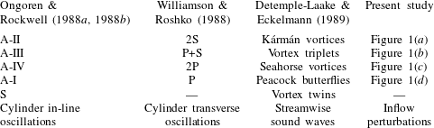
On increasing the amplitude level of perturbation, the induced velocity field gradually takes over control of vortex formation over a wide range of perturbation frequencies. An interesting facet of this behaviour is that there exist several possibilities for vortex shedding to synchronize with perturbations, either symmetrical or antisymmetrical. A number of different patterns or modes of synchronized vortex formation have been found in several experimental and numerical studies (Griffin & Ramberg Reference Griffin and Ramberg1976; Ongoren & Rockwell Reference Ongoren and Rockwell1988b ; Williamson & Roshko Reference Williamson and Roshko1988; Detemple-Laake & Eckelmann Reference Detemple-Laake and Eckelmann1989; Al-Mdallal et al. Reference Al-Mdallal, Lawrence and Kocabiyik2007; Leontini et al. Reference Leontini, Lo Jacono and Thompson2013). In the absence of synchronization, these modes compete with each other, resulting in quasi-periodic or even chaotic wakes (Leontini et al. Reference Leontini, Lo Jacono and Thompson2013). Table 1 provides some classifications of synchronized modes that have appeared in the literature. Ongoren & Rockwell (Reference Ongoren and Rockwell1988b ) distinguished four antisymmetrical modes, denoted as ‘A’, and a symmetrical mode, denoted as ‘S’, in the wake of a streamwise oscillating cylinder at constant amplitude. In the case of sinusoidal cylinder oscillations transverse to a free stream, Williamson & Roshko (Reference Williamson and Roshko1988) introduced a symbolic code of letters and numbers to designate the structure of vortices shed in the wake during a period of oscillation, where ‘S’ signifies a single vortex and ‘P’ signifies a pair of vortices of opposite sign. Detemple-Laake & Eckelmann (Reference Detemple-Laake and Eckelmann1989) also identified various modes and named them after the shape of vortex structures produced in a cylinder wake by superposition of sound waves along the main flow direction, as listed in the third column of table 1. Despite differences in the types of perturbations, as listed in the last row of the table, there are strong similarities between the modes given in each row (note that the table entries are restricted to modes that have similar vortex structures).
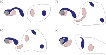
Patterns of synchronized vortex formation in the near wake as depicted by their vorticity fields. Dark blue and light purple contours show negative and positive vorticity above a threshold (normalized value of
 $\pm 1$
). Vortices shed during two consecutive periods of flow perturbation are enclosed by dashed lines, except for case (d) where vortices shed in one period only are visible.

Classifications of patterns of synchronized vortex formation in the published literature.

In the present study, we do not add a new categorization scheme but we find that all antisymmetrical modes listed in table 1 can be induced by manipulating the waveform of perturbations superimposed on the free-stream velocity past a cylinder, in addition to adjusting the amplitude and frequency of perturbations. Figure 1 displays vorticity fields associated with all antisymmetrical modes. In (a), a single vortex is shed from one side during a period of flow perturbation and another single vortex of opposite sign is shed during the next period, resulting in a string of vortices (Detemple-Laake & Eckelmann Reference Detemple-Laake and Eckelmann1989). In (b), an elongated positive vortex is shed from the lower side during a period following a pair of oppositely signed vortices, which were shed from the upper side during the previous period. In (c), a negative and a positive vortex form respectively on the upper and lower side in each period, so that two pairs of vortices (four in total) are shed in the wake over two consecutive periods. Patterns (a)–(c) are
 $P_{2}$
periodic, i.e. are repetitive over two periods. In (d), again a pair of vortices is formed during each period as in (c), but the pair is always shed from the same side of the cylinder; hence, the flow pattern repeats exactly in every period (
 $P_{1}$
periodicity).
In this work, we determine regions in the parameter space of normalized amplitude and frequency where the synchronized modes of figure 1 occur. Furthermore, we show how these modes result from modification of the Kármán vortex street caused by the flow perturbation. We are able to quantify this effect by considering the average generation of circulation on the cylinder surface per period. This stems directly from the component of the relative fluid–solid velocity,
 $-U(t)$
, tangential to the cylinder surface which represents a component of circulation production per unit area (Morton Reference Morton1984). The present simulations allow us to identify how the perturbation velocity controls vortex formation and how subtle changes in the waveform produce different vortex patterns in the wake. Not only the vortex patterns but also, perhaps more importantly, the synchronization regime on the map of normalized amplitude and frequency are modified by the perturbation waveform. The key role of the relative velocity allows generalization of our observations to wakes produced from cylinders oscillating either in line with or transverse to steady incident flows.
The remainder of this paper is organized as follows. Section 2 presents a description of the numerical methodology, the problem kinematics and methods employed for post-processing. Section 3 presents results from numerical simulations on the synchronization regime and corresponding vortex patterns over the map of normalized amplitude and frequency for different perturbation waveforms. Section 4 presents a detailed discussion of the results in terms of the perturbation-induced circulation and the effect of the time-averaged mean velocity, and analogies are drawn to oscillating cylinders. In the last section, the main conclusions from the present study are summarized.
2 Methodology
2.1 Numerical code
The Navier–Stokes equations of fluid motion are formulated on an orthogonal curvilinear grid in two dimensions. The equations have the following general form:
 $$\begin{eqnarray}\displaystyle & & \displaystyle \frac{\unicode[STIX]{x2202}}{\unicode[STIX]{x2202}t}(\unicode[STIX]{x1D70C}\unicode[STIX]{x1D6F7})+\frac{1}{l_{\unicode[STIX]{x1D709}}l_{\unicode[STIX]{x1D702}}}\frac{\unicode[STIX]{x2202}}{\unicode[STIX]{x2202}\unicode[STIX]{x1D709}}(\unicode[STIX]{x1D70C}u_{\unicode[STIX]{x1D709}}l_{\unicode[STIX]{x1D702}}\unicode[STIX]{x1D6F7})+\frac{1}{l_{\unicode[STIX]{x1D709}}l_{\unicode[STIX]{x1D702}}}\frac{\unicode[STIX]{x2202}}{\unicode[STIX]{x2202}\unicode[STIX]{x1D702}}(\unicode[STIX]{x1D70C}u_{\unicode[STIX]{x1D702}}l_{\unicode[STIX]{x1D709}}\unicode[STIX]{x1D6F7})\nonumber\\ \displaystyle & & \displaystyle \quad =\frac{1}{l_{\unicode[STIX]{x1D709}}l_{\unicode[STIX]{x1D702}}}\frac{\unicode[STIX]{x2202}}{\unicode[STIX]{x2202}\unicode[STIX]{x1D709}}\left(\unicode[STIX]{x1D707}\frac{l_{\unicode[STIX]{x1D702}}}{l_{\unicode[STIX]{x1D709}}}\frac{\unicode[STIX]{x2202}\unicode[STIX]{x1D6F7}}{\unicode[STIX]{x2202}\unicode[STIX]{x1D709}}\right)+\frac{1}{l_{\unicode[STIX]{x1D709}}l_{\unicode[STIX]{x1D702}}}\frac{\unicode[STIX]{x2202}}{\unicode[STIX]{x2202}\unicode[STIX]{x1D702}}\left(\unicode[STIX]{x1D707}\frac{l_{\unicode[STIX]{x1D709}}}{l_{\unicode[STIX]{x1D702}}}\frac{\unicode[STIX]{x2202}\unicode[STIX]{x1D6F7}}{\unicode[STIX]{x2202}\unicode[STIX]{x1D702}}\right)+S_{\unicode[STIX]{x1D6F7}},\end{eqnarray}$$
where
 $\unicode[STIX]{x1D70C}$
and
 $\unicode[STIX]{x1D707}$
are the density and viscosity of the fluid respectively,
 $l_{\unicode[STIX]{x1D709}}$
and
 $l_{\unicode[STIX]{x1D702}}$
are spatially varying metric coefficients related to the local orthogonal curvilinear coordinates
 $(\unicode[STIX]{x1D709},\unicode[STIX]{x1D702})$
and
 $(u_{\unicode[STIX]{x1D709}},u_{\unicode[STIX]{x1D702}})$
are the corresponding velocity components in the local coordinates. The generalized variable
 $\unicode[STIX]{x1D6F7}$
is unity for continuity,
 $\unicode[STIX]{x1D6F7}=(u_{\unicode[STIX]{x1D709}},u_{\unicode[STIX]{x1D702}})$
, for momentum equations and
 $S_{\unicode[STIX]{x1D6F7}}$
are source terms including the pressure.
The governing equations are solved numerically using the finite-volume method where all variables are collocated at the grid-cell centres. The original SIMPLE algorithm (Patankar & Spalding Reference Patankar and Spalding1972) is combined with the Rhie–Chow modification (Rhie & Chow Reference Rhie and Chow1983) to avoid chequerboard oscillations in the pressure coupling. A fully implicit first-order Euler discretization of the temporal term is used, a higher-order bounded upwind scheme (Papadakis & Bergeles Reference Papadakis and Bergeles1995) is used for convection terms, while for diffusion terms central differencing is employed.
The computational flow domain is rectangular, extending
 $10D$
upstream,
 $25D$
downstream and
 $10D$
above and below the cylinder (where
 $D$
is the cylinder diameter). The orthogonal curvilinear grid consists of
 $299\times 208$
nodes, which is comparable to other numerical studies employing a rectangular domain (Qu et al.
Reference Qu, Norberg, Davidson, Peng and Wang2013). The solid circle comprises a number of grid cells defined by two adjacent grid lines in the
 $\unicode[STIX]{x1D709}$
direction and a number of grid lines in the
 $\unicode[STIX]{x1D702}$
direction. Velocity is artificially set to zero at these cells to enforce the no-slip boundary condition. At the lateral boundaries of the flow domain, the symmetry boundary condition is employed, whereas a convective boundary condition is employed at the outlet in order to avoid backward reflection of pressure waves. At the inlet of the flow domain, a uniform time-dependent velocity,
 $U(t)$
, is specified, as will be described further below. A non-dimensional time step,
 $\unicode[STIX]{x1D6FF}tU_{\infty }/D$
, of the order of
 $10^{-2}$
is employed in the simulations; this time step satisfies the Courant–Friedrichs–Lewy condition and yields more than 100 steps per vortex-shedding period. The system of discretized equations is solved using a tri-diagonal matrix algorithm (TDMA) with an iterative alternating direction implicit (ADI) method.
2.2 Code verification
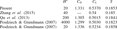
A series of computations were conducted for steady flow past a circular cylinder in order to verify the numerical code. Table 2 shows comparisons of the present results with other published studies in terms of the mean drag coefficient,
 $C_{D}$
, the magnitude of the unsteady lift coefficient,
 $C_{L}$
, and the Strouhal number,
 $S$
, at a Reynolds number of 150. The compared results agree well in most cases; similar agreement has been obtained in the range of Reynolds numbers from 60 to 180. It is worth noting that the lift coefficient is slightly overpredicted in comparison with numerical studies with more than 10 times larger computational domains (
 $H^{\ast }$
is the ratio of the height of the domain to the cylinder diameter in table 2). This is mainly due to the confinement by the lateral boundaries, which is known to have some influence on the flow details and the forces on the cylinder even when the lateral boundaries are hundreds of diameters away from the cylinder (Posdziech & Grundmann Reference Posdziech and Grundmann2007). The study of Posdziech & Grundmann (Reference Posdziech and Grundmann2007) showed that, for a given numerical methodology, the trend is asymptotic. The last row in table 2 shows values computed from asymptotic expressions provided by Posdziech & Grundmann (Reference Posdziech and Grundmann2007) for
 $H^{\ast }=20$
, as in the present study, which agree well with the present results. Behr et al. (Reference Behr, Hastreiter, Mittal and Tezduyar1995) suggested that the lateral boundaries should be at least 16 cylinder diameters apart, which is less than the domain selected in the present study. Thus, we deem that the numerical methodology provides reliable results for the dynamics of the flows under investigation.
Comparison of the present results with other published studies at a Reynolds number of
 $Re=150$
.

2.3 Unsteady problem definition
The time-dependent velocity,
 $U(t)$
, prescribed at the inlet of the flow domain defines the kinematics of the problem. In the present study, the inlet velocity consists of an unsteady periodic component superimposed on a steady component. We are interested in the effect of small deviations of the periodic component from a pure sinusoid. Different velocity waveforms were generated using the following formula:
 $$\begin{eqnarray}U(t)=U_{max}\{\unicode[STIX]{x1D6FD}\pm [1+\unicode[STIX]{x1D6FE}^{2}\sin ^{2}(\unicode[STIX]{x1D714}t+\unicode[STIX]{x1D719})]^{n}\},\end{eqnarray}$$
where
 $\unicode[STIX]{x1D714}$
is the cyclic frequency of the periodic component,
 $\unicode[STIX]{x1D6FE}$
is a parameter related to the amplitude of the velocity perturbations,
 $\unicode[STIX]{x1D6FD}$
and
 $\unicode[STIX]{x1D719}$
are employed to set the maximum velocity in the waveform and its phase respectively, while the index
 $n$
determines the waveform. For
 $n=1$
, the velocity waveform is purely harmonic, i.e. sinusoidal, a case that is employed as the basis for comparisons. For non-harmonic waveforms, the index was set at
 $n=-1$
and two different waveforms were generated using the
 $\pm$
signs in (2.2), denoted hereafter as ‘plus’ and ‘minus’ waveforms respectively. The value of the index
 $n$
was selected on the basis of a preliminary study which has shown that the plus waveform can promote the formation of binary vortices in the wake (Konstantinidis & Bouris Reference Konstantinidis and Bouris2009, Reference Konstantinidis and Bouris2010). The minus waveform was thus employed to inverse the effect of the plus-type waveform.
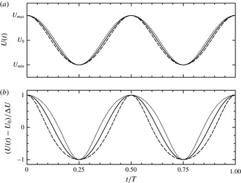
Figure 2(a) shows the general form of the three different velocity waveforms employed in the present study. These can be characterized by the maximum,
 $U_{max}$
, and minimum,
 $U_{min}$
, velocities that occur at the same instant in the perturbation cycle so that direct comparisons can be made for different waveforms. It should be noted that, as per (2.2), each wave repeats itself twice in each nominal period, so that the actual perturbation frequency, denoted
 $f_{e}$
, is twice the nominal, i.e.
 $f_{e}=2f=\unicode[STIX]{x1D714}/\unicode[STIX]{x03C0}$
. The amplitude of velocity perturbations is defined as
 $\unicode[STIX]{x0394}U=(U_{max}-U_{min})/2$
, whose value is determined solely by the
 $\unicode[STIX]{x1D6FE}$
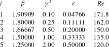
parameter. The simulations were conducted for five different amplitudes listed in table 3.
Waveforms of the inlet velocity,
 $U(t)$
, employed in the present study. Key: ——, sinusoidal waveform; – – –, plus waveform;
 $\cdots \cdots$
, minus waveform.

Summary of the parameters employed in the simulations.

The
 $\unicode[STIX]{x1D6FD}$
parameter is null for the plus waveform, whereas for the minus waveform its value is listed in table 3, so that the maximum instantaneous velocity is exactly the same for all runs reported in this paper;
 $U_{max}$
corresponds to an instantaneous Reynolds number of 180. This was purposely set slightly below the critical value of approximately 190 for the onset of three-dimensional instabilities (Williamson Reference Williamson1996). Hence, the simulated flows are expected to remain two-dimensional at least in the quasi-steady state. This issue has been studied by Kim et al. (Reference Kim, Park, Park, Bae and Yoo2009) for sinusoidal perturbations superimposed on the free-stream velocity. They showed that at
 $Re=220$
, the mode-A instability was suppressed into two-dimensional laminar flow with strong Kármán vortices. Furthermore, Leontini, Thompson & Hourigan (Reference Leontini, Thompson and Hourigan2007) found that the Reynolds number for the onset of three-dimensional instabilities (either mode-A or mode-B) increases above 190 with the amplitude of a cylinder oscillating transverse to a free stream. Therefore, it can be concluded from these studies that three-dimensional instabilities are suppressed in the synchronization range and hence the flows considered in the present study are safely within the two-dimensional regime.
As a consequence of the previous restriction to keep the maximum velocity fixed,
 $U_{min}$
decreases with the perturbation amplitude. Therefore, the median value
 $U_{0}=(U_{max}+U_{min})/2$
, which is common for all three waveforms of the same amplitude, was employed as a suitable reference velocity to calculate the nominal Reynolds number as listed in table 3 and for normalization of the variables.
The distinctive feature of the non-sinusoidal waveforms is the varying duration of high and low velocities, i.e. the velocity distribution is biased with respect to the median velocity. This can be seen more clearly in figure 2(b), which shows a plot of the perturbation velocity normalized with the amplitude. As a result, the probability density function of the perturbation velocity is positively (respectively negatively) skewed for the plus (respectively minus) non-sinusoidal waveforms. This also entails that the time-averaged mean velocity,
 $$\begin{eqnarray}\langle U(t)\rangle =\left(\unicode[STIX]{x1D6FD}\pm \frac{1}{\sqrt{1+\unicode[STIX]{x1D6FE}^{2}}}\right)U_{max},\end{eqnarray}$$
does not exactly coincide with the median velocity, but depends slightly on the waveform. It should be noted that the median velocity is common among different waveforms of the same amplitude. Higher-order statistics of the time-dependent velocity, such as
 $\langle U^{2}(t)\rangle$
, are also affected by the waveform type, and this has some important ramifications, as will be shown in the discussion of the results.
In order to facilitate the compilation and interpretation of the results, we discuss them in terms of the following non-dimensional parameters:
 $$\begin{eqnarray}\unicode[STIX]{x1D700}=\frac{\unicode[STIX]{x0394}U}{U_{0}}\quad \text{and}\quad \unicode[STIX]{x1D6FA}=\frac{\unicode[STIX]{x1D714}}{2\unicode[STIX]{x03C0}f_{v0}},\end{eqnarray}$$
which respectively represent the ratio of the amplitude of the velocity perturbations to the reference velocity and the ratio of the nominal perturbation frequency to the frequency of vortex shedding in unperturbed flow, denoted
 $f_{v0}$
(note that
 $\unicode[STIX]{x1D6FA}=f_{e}/2f_{v0}$
). The unperturbed shedding frequency was computed from an empirical relationship of the Strouhal number as a function of the Reynolds number,
 $S=0.26478{-}0.97229/\sqrt{Re}$
(Williamson & Brown Reference Williamson and Brown1998), where the Reynolds number is based on the reference velocity,
 $U_{0}$
. It should be noted that the convention in the literature is to define the Strouhal number based on the frequency at which single vortices of the same sign are shed from one side of the cylinder. According to the above definitions of
 $\unicode[STIX]{x1D6FA}$
and
 $S$
, the fundamental synchronization occurs in the neighbourhood of
 $\unicode[STIX]{x1D6FA}\approx 1.0$
(i.e.
 $f_{e}=2f\approx 2f_{v0}$
).
2.4 Post-processing
2.4.1 Wake states
The dynamical state of the cylinder wake is characterized by employing time series of the transverse force (lift) as a diagnostic. This is a suitable signal because the lift is free from additional inertial forces acting along the direction of wave propagation, and therefore purely illustrates the integrated effect of vortex dynamics in the wake. It was found that processing of the lift signal in the time domain provided clear distinction between periodic, quasi-periodic and random wake states. On the other hand, the in-line force (drag) was always phase-locked with the flow perturbation and did not distinguish wake states. Lissajous curves, Poincaré maps and phase portraits of the lift signal were employed to further analyse the wake dynamics. Here, we show phase portraits of orthogonal components of the instantaneous lift,
 $C_{L}(t)$
, obtained by
 $$\begin{eqnarray}a(t)=C_{L}(t)\sin (\unicode[STIX]{x1D714}t)\quad \text{and}\quad b(t)=C_{L}(t)\cos (\unicode[STIX]{x1D714}t).\end{eqnarray}$$
Such phase portraits provide information on the instantaneous phase angle,
 $\arctan (b/a)$
, and magnitude,
 $(a^{2}+b^{2})^{1/2}$
, of time-dependent signals with respect to a carrier frequency (Baek & Sung Reference Baek and Sung2000). It should be noted that the nominal perturbation frequency has been employed as the carrier frequency, so that a sinusoidal oscillation at the subharmonic of the actual perturbation frequency yields a limit circle in the
 $a:b$
plane.
2.4.2 Vortex circulation
In order to study the vortex dynamics in more detail, the circulation around individual vortex blobs is quantified using the divergence theorem by numerical surface quadrature of the vorticity field,
 $$\begin{eqnarray}\unicode[STIX]{x1D6E4}=\iint _{A}\unicode[STIX]{x1D701}(x,y)\,\text{d}x\,\text{d}y\approx \mathop{\sum }_{i}\unicode[STIX]{x1D701}_{i}\hat{A}_{i},\end{eqnarray}$$
where
 $\unicode[STIX]{x1D701}$
is the vorticity,
 $A$
is the area of the vortex blob,
 $\unicode[STIX]{x1D701}_{i}$
is the magnitude of the vorticity at a grid-cell and
 $\hat{A}_{i}$
is the area of each grid-cell
 $i$
comprising the blob.
3 Results of numerical simulations
3.1 The primary synchronization range
A major objective of the present study is to demonstrate the effect of different perturbation waveforms on the primary synchronization range, i.e. the envelope in the
 $\unicode[STIX]{x1D6FA}:\unicode[STIX]{x1D700}$
map where antisymmetrical vortex formation is globally synchronized with, or driven by, the posed perturbation. When this occurs, the vortex-shedding frequency locks on to the subharmonic of the actual perturbation frequency,
 $f_{v}=f_{e}/2$
. In this case, the wake state exhibits a
 $P_{2}$
periodicity in the terminology of Leontini et al. (Reference Leontini, Lo Jacono and Thompson2013), where the spatio-temporal symmetry of the wake is completed in every two perturbation periods. This type of synchronization has been the focal point of several studies, and compilations of relevant data can be found in Griffin & Hall (Reference Griffin and Hall1991) and Konstantinidis & Liang (Reference Konstantinidis and Liang2011). It is known that the primary synchronization range depends also on the Reynolds number. Here, we concentrate on low Reynolds numbers in the laminar wake regime.
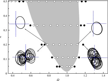
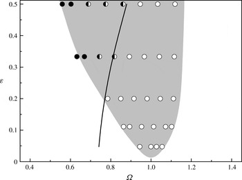
Figure 3 shows the synchronization region in the parameter space of normalized amplitude and frequency for harmonic perturbations, as determined from a large number of simulations at five different amplitudes. At each amplitude, the perturbation frequency was initially set close to
 $\unicode[STIX]{x1D6FA}\approx 1$
and subsequently increased/decreased until vortex synchronization ceased. The boundaries were drawn by fitting a B-spline to points in between periodic and non-periodic states. It should be noted that the apparent threshold amplitude for synchronization is an artefact of the spline fit. The insets show some representative phase portraits for selected cases to illustrate the transition between synchronized, or phase-locked, and non-synchronized modes of vortex formation across the boundaries. The phase portraits corresponding to points inside the shaded region exhibit limit-cycle behaviour whereas those outside exhibit quasi-periodicity. The breadth of the synchronization region increases with the perturbation amplitude while its boundaries are not symmetrical; vortex formation can be synchronized for perturbation frequencies much lower than
 $\unicode[STIX]{x1D6FA}=1$
than for higher values. These features are consistent with several previous studies (Griffin & Hall Reference Griffin and Hall1991; Hall & Griffin Reference Hall and Griffin1993; Al-Mdallal et al.
Reference Al-Mdallal, Lawrence and Kocabiyik2007; Konstantinidis & Bouris Reference Konstantinidis and Bouris2010; Leontini et al.
Reference Leontini, Lo Jacono and Thompson2013). It should be noted that the average Reynolds number decreases with the perturbation amplitude; thus, there might be an implicit
 $Re$
effect on the results.
The primary synchronization regime in the
 $\unicode[STIX]{x1D6FA}:\unicode[STIX]{x1D700}$
map for harmonic perturbations. Open symbols indicate periodic states (circles,
 $P_{2}$
; triangles,
 $P_{1}$
) whereas filled symbols indicate non-periodic states. The insets show representative phase portraits at selected points.

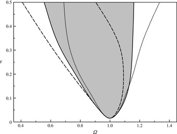
The effect of different perturbation waveforms on the primary synchronization envelope is shown in figure 4. It can be seen that the envelope is skewed towards lower frequencies for perturbations of the plus waveform, whereas it is skewed towards higher frequencies for the minus waveform. The effect is more pronounced at high perturbation amplitudes, while there is only a marginal effect at low amplitudes since all curves originate from
 $\unicode[STIX]{x1D6FA}=1$
. As a consequence, at any particular point in the
 $\unicode[STIX]{x1D6FA}:\unicode[STIX]{x1D700}$
space, the dynamical state of the wake, i.e. whether synchronized or not, depends on the perturbation waveform. This is an important finding from the present study that has several ramifications, as will be shown further below. Theoretically, it might be argued that there is a region in which vortex synchronization is always possible, i.e. for any type of periodic waveform; this will be a narrow band centred around
 $\unicode[STIX]{x1D6FA}\approx 1$
at low amplitudes, which shifts towards lower frequencies with increasing amplitude. This shift indicates that synchronization is a non-linear process.
The effect of different perturbation waveforms on the boundaries of the primary synchronization regime in the
 $\unicode[STIX]{x1D6FA}:\unicode[STIX]{x1D700}$
space: harmonic waveform (solid line), plus waveform (dashed line) and minus waveform (dotted line).

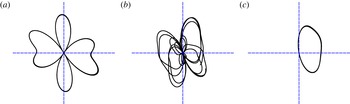
The effect of different perturbation waveforms becomes quite complicated at the highest amplitude because several transitions, not only between synchronized and non-synchronized states but also between different synchronized states, can be observed. Figure 5 shows phase portraits of the transverse force for a particular case that displays such transitions. The harmonic perturbations yield a quasi-periodic state in (b), whereas the non-harmonic perturbations cause phase-locked states; the minus waveform in (a) is associated with
 $P_{1}$
periodicity where the spatio-temporal symmetry of the wake is completed in every perturbation period, whereas in the case of the plus waveform in (c) this is accomplished in every two periods (
 $P_{2}$
periodicity). In the
 $P_{1}$
periodic state, the process of vortex formation becomes so distorted by the imposed perturbation that the phase portrait of the highly modulated transverse force displays an impressive four-ply leaf-like pattern in (a).
Phase portraits of the transverse force at a particular point in parameter space for different perturbations: minus (a), harmonic (b) and plus (c); in all cases,
 $\unicode[STIX]{x1D6FA}=0.52,\unicode[STIX]{x1D700}=0.50$
.

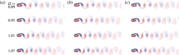
Instantaneous patterns of synchronized vortex formation for different perturbation waveforms at different frequencies and a low amplitude of
 $\unicode[STIX]{x1D700}=0.111$
: minus (a), harmonic (b) and plus (c). Blue and red shading show negative and positive vorticity respectively.

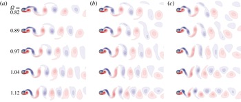
Instantaneous patterns of synchronized vortex formation for different perturbation waveforms at different frequencies and a high amplitude of
 $\unicode[STIX]{x1D700}=0.333$
: minus (a), harmonic (b) and plus (c). Blue and red shading show negative and positive vorticity respectively.

3.2 Patterns of synchronized vortex formation
The patterns of synchronized vortex formation in the wake were examined by producing animations of the instantaneous vorticity distributions from each simulation. The results show that a regular pattern of vortex formation of single vortices alternately on each side occurs at low amplitudes, whereas more complex patterns arise at high amplitudes. Figures 6 and 7 show some representative pictures of the instantaneous patterns at low and high amplitudes respectively. In all figures, each frame corresponds to the instant of the maximum inflow velocity for easier comparison among different cases.
At a low amplitude of
 $\unicode[STIX]{x1D700}=0.111$
, only the familiar Kármán mode where single vortices form alternately on each side of the cylinder can be observed (figure 6). A single vortex is shed from one side during one period and then another single vortex of the opposite sign is shed from the other side during the next period, leading to the Kármán vortex street as in the unperturbed cylinder wake. Nonetheless, the perturbation frequency has a controlling effect on the arrangement of the vortices and slightly on their strength. As
 $\unicode[STIX]{x1D6FA}$
increases (looking in each panel from top to bottom), more vortices are shed per unit time due to synchronization, which become more squeezed as the longitudinal distance between them decreases. The smaller vortex area causes a slight decrease in the strength of the first-released vortex from the cylinder, as confirmed by computing the surface quadrature of the vorticity in each individual vortex. Further downstream, at 10 diameters from the cylinder centre, the vortex strength attains a normalized value of approximately
 $\unicode[STIX]{x03C0}$
in all cases. The latter value is similar to the vortex strength in the unperturbed cylinder wake in the same range of Reynolds numbers (Green & Gerrard Reference Green and Gerrard1993). The effect of different perturbation waveforms (looking at frames in the same row) on the vorticity distribution is hardly detectable at low amplitudes, although a detailed examination of the circulation and trajectory of the vortices reveals some systematic trends (not discussed in detail here for economy of space).
At a high amplitude of
 $\unicode[STIX]{x1D700}=0.333$
, vortices still form alternately on each side but there is additional vorticity trailing behind each main vortex forming in the very near wake, particularly for the lower perturbation frequencies (see the top row in figure 7). For harmonic perturbations, the trailing vorticity behind each positive vortex is dissolved, whereas the trailing vorticity behind each negative vortex separates from the stronger vortex core and moves independently upwards as it is convected downstream. The main positive and negative vortices pair together and move downwards while they are convected downstream. This pattern of vortex formation has been previously observed in symmetrically perturbed wakes (Ongoren & Rockwell Reference Ongoren and Rockwell1988b
; Meneghini & Bearman Reference Meneghini and Bearman1995; Leontini et al.
Reference Leontini, Lo Jacono and Thompson2013) and is similar to the ‘P+S’ mode – following the naming convention of Williamson & Roshko (Reference Williamson and Roshko1988) – observed in the wake of cylinders oscillating at high amplitude transverse to a free stream. As
 $\unicode[STIX]{x1D6FA}$
increases (looking in figure 7(b) from top to bottom), the trailing vorticity becomes less pronounced, leading to a more Kármán-like configuration downstream. At this high amplitude, the effect of different perturbation waveforms now becomes evident. The minus waveform induces less trailing vorticity behind each main vortex, leading to a pattern of single vortices downstream (see figure 7
a), whereas the plus waveform promotes the generation of trailing vorticity, leading to the formation of binary vortices near the cylinder (see figure 7
c). The arrangement of the binary vortices in the wake produces a pattern that bears some similarities to the ‘2P’ mode of Williamson & Roshko (Reference Williamson and Roshko1988). The configuration of binary vortices cannot be sustained as they move downstream and rearranges to either a single vortex and a pair at low frequencies or solitary vortices at high frequencies. Irrespective of the perturbation waveform, increasing
 $\unicode[STIX]{x1D6FA}$
tends to reduce the amount of vorticity trailing behind each main vortex so that, for the highest perturbation frequency, only the basic pattern of single vortices can be observed in the wake. Yet, the perturbation waveform affects the lateral distance (i.e. normal to the flow direction) between successive vortices of opposite sign; a slight increase in the lateral distance can be observed in going from the minus to the harmonic to the plus waveforms (from (a) to (c)) in figure 7.
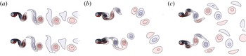
Instantaneous patterns of vortex formation at the instant of maximum inflow velocity over two consecutive perturbation periods for three perturbation waveforms
 $(\unicode[STIX]{x1D6FA}=0.52,\unicode[STIX]{x1D700}=0.5)$
: minus (a), harmonic (b) and plus (c). Blue and red shading show negative and positive vorticity respectively.

At the highest amplitude of
 $\unicode[STIX]{x1D700}=0.5$
examined, modes of synchronized vortex formation emerge that do not necessarily exhibit the
 $P_{2}$
periodicity, as already pointed out. Figure 8 shows representative patterns at approximately the instant of maximum inflow velocity over two consecutive perturbation periods (i.e. one nominal period of perturbation) that correspond to the same point in the
 $\unicode[STIX]{x1D6FA}:\unicode[STIX]{x1D700}$
space for all three waveforms. For harmonically perturbed flow, the vortex pattern in the first period differs completely from that in the next period in terms of the number of vortices and their location in the wake. Furthermore, the formation of opposite-sign vortices at the back of the cylinder is asymmetrical in the first instant whereas it is nearly symmetrical in the second instant. It can be inferred from these non-repetitive wake patterns that vortex formation is not synchronized, but the wake is in a quasi-periodic state where the patterns nearly repeat over multiple perturbation cycles (Leontini et al.
Reference Leontini, Lo Jacono and Thompson2013). For perturbations of the minus waveform, the same pattern is observed at both instants: a pair of vortices of opposite sign is shed from one side during each perturbation period, i.e. the shedding frequency synchronizes with the actual perturbation frequency,
 $f_{v}=f_{e}$
. Each vortex pair is deflected downwards from the wake centreline as it is convected away from the cylinder. This asymmetrical wake induces a non-zero mean lift of considerable magnitude, in this case
 $C_{L\mathit{mean}}\approx 0.3$
. The existence and appearance of this mode of vortex formation that is
 $P_{1}$
periodic are consistent with the findings of Leontini et al. (Reference Leontini, Lo Jacono and Thompson2013). They suggested that this mode is possible, for sinusoidal driving waveforms, for perturbation frequencies just below the Strouhal frequency. Here, we observe this mode at a slightly higher frequency as the velocity perturbation is non-sinusoidal. This pattern resembles the ‘P’ mode observed in the wakes of transversely oscillating cylinders (Williamson & Roshko Reference Williamson and Roshko1988). For the plus waveform, finally, an entirely different vortex pattern emerges where pairs of opposite-sign vortices are shed during each perturbation period: a pair of opposite-sign vortices is shed during one period and a mirror-image pair is shed during the next period. The initial formation of the oppositely signed vortices is nearly symmetrical on both sides (not evident for the instants shown), but one of these vortices grows larger and sheds ahead of the other; in the next period the order is reversed. This antisymmetrical shedding of vortex pairs causes the lift to change sign in each perturbation period. As a result, this wake state exhibits the
 $P_{2}$
periodicity. The switch to this wake mode can be explained by the shift of the primary synchronization range towards lower frequencies in the case of the plus waveform.
4 Discussion
4.1 Rate of vorticity generation
The modification of vortex patterns in the cylinder wake induced by perturbations in the velocity can be explained on the basis of vorticity generation at the cylinder surface. The flux density of vorticity out of the cylinder surface is given by
 $$\begin{eqnarray}-\unicode[STIX]{x1D708}\boldsymbol{n}\boldsymbol{\cdot }\unicode[STIX]{x1D735}\unicode[STIX]{x1D73B}=-\unicode[STIX]{x1D70C}^{-1}(\boldsymbol{n}\times \unicode[STIX]{x1D735})p-\boldsymbol{n}\times \text{d}\boldsymbol{U}/\text{d}t,\end{eqnarray}$$
where all terms are evaluated at the fluid–solid boundary,
 $\unicode[STIX]{x1D73B}$
is the vorticity vector,
 $\boldsymbol{n}$
is the surface-normal unit vector,
 $p$
is the pressure and
 $\boldsymbol{U}$
is the relative velocity vector between the cylinder and the free stream (see Morton Reference Morton1984). Therefore, the vorticity production at the surface involves two mechanisms associated with tangential pressure gradients and surface acceleration. The first mechanism is active in both unperturbed and perturbed flows, and in the former case yields a constant flux of vorticity of both signs from the cylinder surface (Xu, Zhou & Wang Reference Xu, Zhou and Wang2006). The process of vortex shedding is related to the redistribution of the generated vorticity through its advection and diffusion. Typically, only a fraction of the vorticity generated at the cylinder surface, approximately half of it, is found in the Kármán vortices shed in the wake (Griffin & Ramberg Reference Griffin and Ramberg1974, Reference Griffin and Ramberg1976). The second mechanism requires the existence of relative acceleration between the fluid and the body. For an impulsive change of the relative velocity, the second term adds an amount of circulation proportional to
 $\unicode[STIX]{x1D6FF}U$
. It should be noted that a change in the sign of
 $\unicode[STIX]{x1D6FF}U$
does not represent a sink of vorticity but rather a source of vorticity of the opposite sign (Morton Reference Morton1984). In the present configuration, we posit that the superposition of flow perturbations does not affect the former mechanism significantly but additional vorticity of both signs is generated via the latter mechanism.
The rate at which circulation (of each sign) flows in the free shear layers separating on each side of the cylinder can be estimated by
 $$\begin{eqnarray}\dot{\unicode[STIX]{x1D6E4}}={\textstyle \frac{1}{2}}u_{s}^{2}(t),\end{eqnarray}$$
where
 $u_{s}$
is the velocity at the edge of the boundary layer on separation (Griffin Reference Griffin1978). The origin of the above relationship is the hodograph free-streamline theory (Roshko Reference Roshko1954). In steady flow past a cylinder, the average value of
 $u_{s}$
can be expressed as
 $u_{s}=\unicode[STIX]{x1D705}U_{\infty }$
, where
 $U_{\infty }$
is the free-stream velocity and
 $\unicode[STIX]{x1D705}$
is a constant factor that depends on the Reynolds number. The base pressure coefficient at the back stagnation point of the cylinder is related to
 $\unicode[STIX]{x1D705}$
through
 $\unicode[STIX]{x1D705}^{2}=1-C_{pb}$
. In time-dependent flow, the instantaneous value of
 $u_{s}$
cannot be expressed simply as
 $u_{s}(t)=\unicode[STIX]{x1D705}U(t)$
as the velocity at the edge of separation has, at least, components at the perturbation frequency,
 $f_{e}$
, and the vortex-shedding frequency,
 $f_{v}$
, where typically
 $f_{v}=f_{e}/2$
in the primary synchronization range. As both
 $U(t)$
and
 $u_{s}(t)$
are periodic, they can be expressed in series, and thus we may write
 $U(t)=\sum _{i}U_{i}\cos (\text{i}\unicode[STIX]{x1D714}t)$
and
 $u_{s}(t)=\sum _{i}u_{i}\cos (\text{i}\unicode[STIX]{x1D714}t+\unicode[STIX]{x1D719}_{i})$
. Integration of (4.2) over a vortex-shedding period,
 $T$
, yields
 $$\begin{eqnarray}\unicode[STIX]{x1D6E4}={\textstyle \frac{1}{2}}\unicode[STIX]{x1D705}^{2}\langle U^{2}\rangle T,\end{eqnarray}$$
where
 $\unicode[STIX]{x1D705}^{2}=\sum u_{i}^{2}/\sum U_{i}^{2}=\langle u_{s}^{2}(t)\rangle /\langle U^{2}(t)\rangle$
is a factor that depends on the flow details around the cylinder and related pressure gradients, i.e.
 $\unicode[STIX]{x1D705}$
depends on
 $\unicode[STIX]{x1D6FA}$
,
 $\unicode[STIX]{x1D700}$
and
 $Re$
. Our previous argument on vorticity generation suggests that perturbations in the velocity have a direct effect on the circulation through
 $\langle U^{2}\rangle$
and an indirect effect through
 $\unicode[STIX]{x1D705}$
. Hence, we may artificially separate these effects by looking into the first term while ignoring variations in the second term.
In the primary synchronization range where subharmonic lock-on occurs (
 $P_{2}$
periodicity), the period of vortex shedding is controlled by the perturbation frequency, i.e.
 $T=2T_{e}$
. Assuming a harmonically perturbed free stream of the simple form
 $U(t)=U_{0}[1+\unicode[STIX]{x1D700}\cos (2\unicode[STIX]{x03C0}f_{e}t)]$
, then the result of the integration can be written in non-dimensional terms as
 $$\begin{eqnarray}\unicode[STIX]{x1D6E4}^{\ast }=\frac{\unicode[STIX]{x1D705}^{2}}{2\unicode[STIX]{x1D6FA}S}\left(1+\frac{\unicode[STIX]{x1D700}^{2}}{2}\right),\end{eqnarray}$$
where
 $S=f_{v0}D/U_{0}$
is the Strouhal number for unperturbed flow past a fixed cylinder. The above result shows that the circulation generated at the cylinder surface over a shedding cycle is inversely proportional to the perturbation frequency and increases with the square of the perturbation amplitude.
The above simple expression is very consistent with observed vortex patterns as functions of perturbation amplitude and frequency. That is, the appearance of extra vorticity trailing behind main vortices, sometimes as secondary vortex entities, is much more pronounced for low
 $\unicode[STIX]{x1D6FA}$
values and for high
 $\unicode[STIX]{x1D700}$
values (see figures 6 and 7). These trends were consistently observed with perturbation amplitude and frequency for all waveforms. On the other hand, the vorticity distributions for different waveforms appear to contradict the behaviour predicted by expression (4.3) which shows that the circulation released into the wake over a shedding cycle scales with
 $\langle U^{2}\rangle$
. The latter quantity has a higher value for the minus waveform than for the plus waveform, with the harmonic waveform having an intermediate value. However, the plus waveform appears to generate more wake vorticity in the form of binary vortices whereas the minus waveform appears to generate less wake vorticity (single vortices), as has been shown earlier.
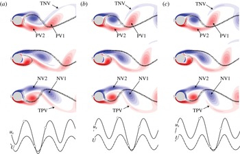
We examine the above contradiction by looking more closely into the development of the shear layers at three instants over half of a vortex-shedding cycle (one actual perturbation period) in figure 9. The sequence of streamlines and instantaneous vorticity distributions shows a flip-flopping wake that has the same basic characteristics as the unperturbed cylinder wake, for which a physical model was suggested a long time ago by Gerrard (Reference Gerrard1966). More specifically, the shear layer from the lower side folds towards the upper side, remaining nearly attached to the back of the cylinder at the first instant. In this way, the vorticity supplied to the negative vortex growing on the upper side is cut off from its generator. At the following instant, the lower shear layer is no longer attached to the back of the cylinder. Instead, it separates nearly parallel to the flow direction but folds back towards the cylinder in a short distance. During this stage, a secondary negative vortex has formed in the shear layer on the upper side while the main positive vortex has formed on the lower side. The flapping motion of the upper shear layer towards the lower side completes the half-cycle, and a mirrored image of this process is repeated during the next half-cycle of vortex shedding.
Streamlines superposed on vorticity distributions at three instants over half of a vortex-shedding cycle for different perturbation waveforms: minus (a), harmonic (b) and plus (c). In all cases,
 $\unicode[STIX]{x1D6FA}=0.785,\unicode[STIX]{x1D700}=0.2$
. Blue and red shading show negative and positive vorticity respectively. The time traces on the lower plots show the inflow velocity,
 $U(t)$
(dashed lines), and the velocity,
 $u_{s}(t)$
(solid lines), near the edge of the separating shear layer on the upper side,
 $\{x/D,y/D\}=\{0,0.7\}$
.

The above development appears to be very similar for all three perturbation waveforms. However, there are subtle differences along the process that can be identified in some flow details. For instance, the strand of elongated vorticity trailing behind the negative vortex (respectively positive vortex) that moves out of the field of view at the first (respectively third) instant, indicated as TNV (respectively TPV) in figure 9, connects all the way back to the following negative vortex (respectively positive vortex) nearer the cylinder but is thicker for the minus waveform than it is for the harmonic waveform. On the contrary, in the case of the plus waveform the trail of the downstream negative vortex TNV (respectively TPV), which is still visible at the first (respectively third) instant, does not connect back to the subsequent negative (respectively positive) vortex near the cylinder.
A careful examination of the formation region reveals that two interconnected but distinct vortices of the same sign emerge on each side of the cylinder over part of the perturbation cycle. At the instant shown in the upper row in figure 9, two positive vortices indicated PV1 and PV2 have formed on the lower side. Similarly, during the next half-period two negative vortices NV1 and NV2 have formed on the upper side, as shown in the third row. The circulation of these distinct vortex blobs that spring out from the cylinder was measured by interactively locating the area of each vortex on the computer screen. This area terminated at the neck connecting the vortex (PV2, NV2) to the cylinder on the upstream side and at the neck connecting one vortex (PV1, NV1) to the next one (PV2, NV2) on the downstream side. For these strongly interconnected binary vortices, the vortex area and circulation was measured independently for each vortex blob and the sum was computed. Table 4 shows the results for the case in figure 9. The results show that the maximum circulation in the vortex-formation region is considerably higher for the minus waveform than for the plus waveform, which is consistent with expression (4.3). Thus, the previously mentioned contradiction only appears when looking at the wake region and can be explained by the fact that in the case of the minus waveform vortices lose their strength more rapidly and end up with less circulation immediately after being shed than in the case of the plus waveform. As a consequence, the circulation of isolated wake vortices 10 diameters downstream from the cylinder centre is slightly lower for the minus waveform than for the plus one (see table 4).
We hypothesize that circulation is lost by cross-diffusive annihilation of oppositely signed vorticity in the formation region. It seems that the perturbation velocity of the minus waveform, which accelerates more steeply towards the maximum velocity, causes the primary positive vortex on the lower side to catch up with the secondary negative vortex on the upper side, and they thereby cancel each other out by cross-diffusion (see figure 9). As a result, the amount of vorticity that survives vortex formation crucially depends on the detailed process, which in turn depends on the perturbation amplitude, frequency and waveform. It should be pointed out that despite the binary vortex formation process shown more closely in figure 9, the resulting vortex patterns in the wake comprise only single vortices. On the other hand, the same process leads to substantially different vortex patterns at high amplitudes that critically depend on the waveform, e.g. as in figure 7.
Vortex circulation,
 $\unicode[STIX]{x1D6E4}^{\ast }$
, for the case
 $\unicode[STIX]{x1D6FA}=0.785,\unicode[STIX]{x1D700}=0.2$
.

The binary vortex formation process described above is clearly the result of the imposed velocity perturbation. A simple model may be devised along the line of reasoning of vorticity generation, to predict when both primary and secondary vortices resulting from this binary process can survive the formation region and appear in the wake. We posit that vorticity will end up as an entity in the near wake if the circulation generated in one perturbation cycle exceeds a threshold (e.g. a minimum energy level). Thus, an appropriate threshold may be the value of the circulation in the unperturbed wake, i.e.
 $\unicode[STIX]{x1D6E4}_{min}^{\ast }\approx \unicode[STIX]{x03C0}$
. Integrating (4.2) over a perturbation cycle, that is half of a vortex-shedding cycle, and equating the result to the latter minimum yields the following criterion:
 $$\begin{eqnarray}\unicode[STIX]{x1D700}\geqslant \sqrt{\frac{8\unicode[STIX]{x03C0}S\unicode[STIX]{x1D6FA}}{\unicode[STIX]{x1D705}^{2}}-2}.\end{eqnarray}$$
Figure 10 shows a map of patterns of synchronized vortex formation for harmonic perturbations in parameter space along with the criterion in (4.5). It can be seen that the criterion divides the map into regions where the shedding of solitary or binary vortices occurs with satisfactory agreement. The results thus support the hypothesis that primary and secondary vortices survive the formation region when the velocity perturbations can produce sufficient circulation in each perturbation cycle. It should be noted that
 $\unicode[STIX]{x1D705}$
has been assumed to be constant in the criterion, whereas in fact
 $\unicode[STIX]{x1D705}$
depends on
 $\unicode[STIX]{x1D6FA}$
,
 $\unicode[STIX]{x1D700}$
and
 $Re$
, which might account for small deviations from observations. Nevertheless, the purpose here is to make a qualitative comparison since the value of
 $\unicode[STIX]{x1D6E4}_{min}$
is also subjective. It should also be noted that the binary vortices found in the formation region, once shed, tend to rearrange, leading to a vortex street with either a single vortex and a pair of vortices or two single vortices further downstream. Therefore, the interpretation of a particular pattern also depends on the field of view.
Map of vortex patterns in the
 $\unicode[STIX]{x1D6FA}:\unicode[STIX]{x1D700}$
space juxtaposed on the primary synchronization envelope for harmonically perturbed flow: single vortices (open symbols), a single and a vortex pair (semi-filled symbols) and vortex pairs (full symbols). The solid line represents the criterion in (4.5) for the segregation of regions where the shedding of binary vortices is expected.

4.2 Effect of time-averaged mean velocity on synchronization range
As mentioned in the introduction, an important issue for a wide class of unsteady bluff-body flows with vortex shedding that we wish to explore is what the kinematical parameters that control vortex formation are. The velocity,
 $u_{s}(t)$
, at the edge of the separation points appears to be an important factor as it determines the amount of vorticity shed in the wake. It is interesting to note here that periodic vortex shedding induces a fluctuating velocity,
 $u_{s}(t)$
, even when the incident flow is steady. Our analysis indicates that for vortex shedding to synchronize with the imposed perturbations, the perturbation velocity must cooperate with the fluctuating velocity associated with vortex shedding, e.g. the minimum of
 $U(t)$
must coincide in time with the minimum of
 $u_{s}(t)$
. The time traces shown at the bottom of figure 9 illustrate this connection. Furthermore, Jeon & Gharib (Reference Jeon and Gharib2004) suggested that a universal vortex formation time governs when a lump of vorticity separates from a region of concentrated vorticity in free shear layers. The vortex-formation time scales with the distance travelled by the body in a shedding period,
 $x_{travel}=UT$
. It follows naturally that
 $x_{travel}=\langle U(t)\rangle T$
in time-dependent flows. Then, the time-averaged mean velocity must have a controlling effect on the process of vortex formation.
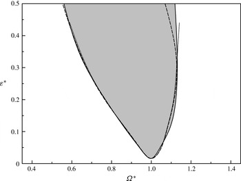
The present results can be used to verify the idea that the time-averaged mean velocity plays some role in the vortex formation process since different perturbation waveforms considered in this study have different time-averaged mean velocities. Figure 11 shows the primary synchronization range in the parameter space of modified frequency and amplitude,
 $\unicode[STIX]{x1D6FA}^{\ast }:\unicode[STIX]{x1D700}^{\ast }$
, where instead of the median velocity,
 $U_{0}$
, now the mean velocity,
 $\langle U(t)\rangle$
, is employed as a reference velocity for normalization, i.e.
 $$\begin{eqnarray}\unicode[STIX]{x1D700}^{\ast }=\frac{\unicode[STIX]{x0394}U}{\langle U\rangle }\quad \text{and}\quad \unicode[STIX]{x1D6FA}^{\ast }=\frac{\unicode[STIX]{x1D714}D}{2\unicode[STIX]{x03C0}S\langle U\rangle },\end{eqnarray}$$
where in turn the Strouhal number is computed as a function of the Reynolds number based on the mean velocity,
 $\langle U\rangle D/\unicode[STIX]{x1D708}$
. It can be seen that the boundaries of the synchronization envelope in the modified
 $\unicode[STIX]{x1D6FA}^{\ast }:\unicode[STIX]{x1D700}^{\ast }$
map collapse very well for different perturbation waveforms. This provides support to the idea that vortex formation is governed by the same time scale (expressed as distance travelled). It should be pointed out that the collapse of the data is primarily due to the change in the reference velocity, whereas the implicit change in the Strouhal number has only a minor effect on the outcome.
The primary synchronization envelope in the
 $\unicode[STIX]{x1D6FA}^{\ast }:\unicode[STIX]{x1D700}^{\ast }$
space: harmonic waveform (solid line), plus waveform (dashed line) and minus waveform (dotted line).

4.3 Harmonic cylinder oscillations in a steady free stream
The purpose here is to generalize the present findings for periodically perturbed flows past a fixed cylinder and extrapolate them to the more widely studied problem of cylinders oscillating in a steady free stream. This expands on the idea that primarily the kinematics of the relative velocity between the cylinder and the free stream controls vortex formation.
4.3.1 In-line oscillations
The connection between the perturbed flows considered in the present study and cylinders oscillating in line with a free stream of steady velocity is straightforward, as the two problems are kinematically equivalent. Dynamically, the only difference is that in a time-dependent flow there is an additional force due to dynamic buoyancy (Froude–Krylov term) induced by the propagation of pressure waves. The relative velocity induced by in-line oscillations is simply
 $U(t)=U_{\infty }-{\dot{x}}_{c}(t)$
, where
 ${\dot{x}}_{c}(t)$
is the instantaneous velocity of the cylinder and
 $U_{\infty }$
is the free-stream speed. Thus, the present results can be directly applied to in-line oscillating cylinders by a simple transformation of variables as required, e.g. for sinusoidal oscillations,
 $x_{c}(t)=A\sin (\unicode[STIX]{x1D714}_{x}t)$
, the perturbation parameters can be obtained as
 $$\begin{eqnarray}\unicode[STIX]{x1D6FA}=\frac{\unicode[STIX]{x1D714}_{x}D}{4\unicode[STIX]{x03C0}SU_{\infty }}\quad \text{and }\quad \unicode[STIX]{x1D700}=\frac{\unicode[STIX]{x1D714}_{x}A}{U_{\infty }}.\end{eqnarray}$$
It should be noted that for sinusoidal in-line oscillations in a steady free stream,
 $\langle U\rangle =U_{\infty }$
, hence
 $\unicode[STIX]{x1D6FA}^{\ast }=\unicode[STIX]{x1D6FA}$
and
 $\unicode[STIX]{x1D700}^{\ast }=\unicode[STIX]{x1D700}$
.
The present study is complementary to previous numerical studies with in-line oscillating cylinders (Al-Mdallal et al. Reference Al-Mdallal, Lawrence and Kocabiyik2007; Leontini et al. Reference Leontini, Lo Jacono and Thompson2013). In particular, Leontini et al. (Reference Leontini, Lo Jacono and Thompson2013) considered in detail the wake states and frequency selection in the parameter space up to the lower boundary of the synchronization range. The present results are consistent with their findings in terms of wake states and patterns of vortex formation for overlapping regions in the normalized amplitude–frequency map, as commented earlier in the presentation of the results.
Our analysis shows that, within the synchronization range, the circulation of each sign released into the wake during each shedding cycle increases with
 $\unicode[STIX]{x1D700}$
. As positive and negative vorticity must be produced at the same rate due to the conservation of total vorticity (Morton Reference Morton1984), the perturbation-induced circulation will completely surpass that generated by regular vortex formation at some amplitude. Then, symmetrical vortex formation leads to the simultaneous shedding of twin vortices from both sides of the cylinder, as demonstrated in previous studies (Marzouk & Nayfeh Reference Marzouk and Nayfeh2009; Leontini et al.
Reference Leontini, Lo Jacono and Thompson2013; Liu & Feng Reference Liu and Feng2015). The present study did not extend to very high amplitudes, where the purely symmetrical shedding mode can be induced, but initial signs of this mode can be seen, e.g. see the bottom of figure 8(b). We note the symmetrical shedding mode, although not directly relevant to the present study, as it illustrates the effect of perturbations in the relative velocity that may be overlooked when considering the amplitude of cylinder oscillation as the governing kinematic parameter. For instance, if the amplitude of the velocity perturbation exceeds the free-stream velocity, i.e.
 $\unicode[STIX]{x1D700}>1$
, the flow reverses over part of the cycle and the motion-induced circulation on each side of the cylinder temporarily changes sign. Then, more complex patterns can be generated due to this mechanism, e.g. symmetric binary vortex streets (Xu et al.
Reference Xu, Zhou and Wang2006).
4.3.2 Transverse oscillations
The resemblance of the patterns of synchronized vortex formation observed in the present study to those observed in wakes of cylinders undergoing transverse oscillations has already been noted. In particular, we have found similarities to the 2S, P+S, 2P and P modes, following the symbolic naming of Williamson & Roshko (Reference Williamson and Roshko1988). However, what exactly is the relation between these modes and the shedding of solitary and binary vortices observed in the present study in terms of the kinematics?
Map of vortex patterns found in the present study transformed into the
 $\unicode[STIX]{x1D706}^{\ast }:A^{\ast }$
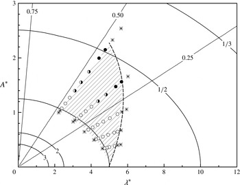
space corresponding to transverse harmonic oscillations: solitary vortices (open symbols), a solitary and a binary vortex (semi-filled symbols), binary vortices (full symbols) and non-synchronized vortex formation (star symbols). The circumferential lines indicate isocontours of the
 $\unicode[STIX]{x1D6FA}^{\ast }$
parameter and the radial lines indicate icocontours of the
 $\unicode[STIX]{x1D700}^{\ast }$
parameter.

The connection of the present flow configuration to that of a cylinder oscillating transversely in a free stream poses some challenges. Consider a cylinder as it sinusoidally oscillates transverse to a free stream of constant speed
 $U_{\infty }$
, its displacement given by
 $y_{c}(t)=A\sin (\unicode[STIX]{x1D714}_{y}t)$
. In this case, the relative velocity vector between the cylinder and the free stream changes periodically in both direction and magnitude. The magnitude of the relative velocity is
 $$\begin{eqnarray}U(t)=U_{\infty }\sqrt{1+\unicode[STIX]{x1D6FC}^{2}\cos ^{2}\unicode[STIX]{x1D714}_{y}t},\end{eqnarray}$$
where
 $\unicode[STIX]{x1D6FC}=\unicode[STIX]{x1D714}_{y}A/U_{\infty }$
is the ratio of the maximum transverse velocity of the cylinder to the velocity of the free stream. Inspection of (4.8) shows that it represents a waveform similar to (2.2) of the minus type, with
 $n=-1/2$
. Thus, it is possible to relate both configurations in terms of the kinematical parameters,
 $$\begin{eqnarray}\unicode[STIX]{x1D6FA}^{\ast }=\frac{\unicode[STIX]{x1D714}_{y}D}{2\unicode[STIX]{x03C0}SU_{\infty }\unicode[STIX]{x1D70E}_{1}}\quad \text{and}\quad \unicode[STIX]{x1D700}^{\ast }=\frac{\sqrt{1+\unicode[STIX]{x1D6FC}^{2}}-1}{2\unicode[STIX]{x1D70E}_{1}},\end{eqnarray}$$
where
 $\unicode[STIX]{x1D70E}_{1}=\langle U\rangle /U_{\infty }$
is a correction factor for the mean velocity that plays a key role in the transformation of variables. The inverse transformation to the parameter space employed in driven oscillation studies, where typically the normalized amplitude
 $(A^{\ast }=A/D)$
and wavelength
 $(\unicode[STIX]{x1D706}^{\ast }=U_{\infty }/fD)$
are employed, the relations being
 $$\begin{eqnarray}\unicode[STIX]{x1D706}^{\ast }=\frac{1}{\unicode[STIX]{x1D6FA}^{\ast }\unicode[STIX]{x1D70E}_{1}S}\quad \text{and}\quad A^{\ast }=\frac{\sqrt{(1+2\unicode[STIX]{x1D700}^{\ast }\unicode[STIX]{x1D70E}_{1})^{2}-1}}{2\unicode[STIX]{x03C0}\unicode[STIX]{x1D6FA}^{\ast }\unicode[STIX]{x1D70E}_{1}S},\end{eqnarray}$$
is equally useful.
Figure 12 shows a map of vortex patterns observed in the present study transformed into the
 $\unicode[STIX]{x1D706}^{\ast }:A^{\ast }$
space. On this map, circumferential lines indicate isocontours of the
 $\unicode[STIX]{x1D6FA}^{\ast }$
parameter, drawn assuming a constant Strouhal number of
 $S=0.2$
, and radial lines indicate isocontours of the
 $\unicode[STIX]{x1D700}^{\ast }$
parameter. Ponta & Aref (Reference Ponta and Aref2005) provided a theoretical basis for the vortex synchronization regions of transversely oscillating cylinders with reference to a map similar to the one shown in figure 12. Although the circumferential lines shown here are essentially the same as those on their map, our starting point for deriving these lines is quite different, i.e. the change in the time-averaged mean velocity with the kinematical parameters of the oscillation. Furthermore, the present analysis shows that the radial lines, which bound certain regions where different modes appear, represent the effect of the amplitude of perturbation in the relative velocity; mode changes can be readily attributed to variations in the cycle-averaged circulation production with
 $\unicode[STIX]{x1D6FA}^{\ast }$
and
 $\unicode[STIX]{x1D700}^{\ast }$
, as explained in the foregoing discussion.
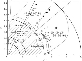
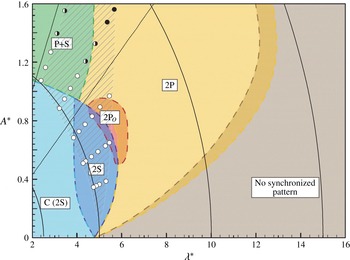
Comparison of the vortex patterns from the present study overlaid on the map of modes from Williamson & Roshko (Reference Williamson and Roshko1988). The symbols are as in figure 12.

Comparison of the vortex patterns in the
 $\unicode[STIX]{x1D706}^{\ast }:A^{\ast }$
map from the present study with that from Morse & Williamson (Reference Morse and Williamson2009). Coloured regions separated by dashed lines indicate different vortex modes from their study. The symbols are as in figure 12.

In figure 13, the vortex patterns from the present study are overlaid on the original map of modes by Williamson & Roshko (Reference Williamson and Roshko1988). There is remarkable qualitative agreement between the results. Quantitatively, their region of the 2S mode corresponds to points identified here as shedding of solitary vortices; points identified here as shedding of binary vortices correspond to the 2P mode; points where one of the binary vortices fuses into a solitary vortex while the other one splits into two vortices downstream correspond to the region of the P+S mode. Some points where the shedding of solitary vortices has been observed in the present study correspond to regions of the 2P and P+S modes in the original map. However, on a map of modes produced more recently based on force measurements (Morse & Williamson Reference Morse and Williamson2009) most of the latter points do correspond to a region where the 2S mode resides. A direct comparison with this latter study is provided in figure 14. Thus, we consider that the origin of different vortex patterns for transversely oscillating cylinders can be explained well in terms of the effect of amplitude and frequency of perturbations in the relative velocity, imposed by an oscillating cylinder, since the present regime map is consistent with findings from the published literature.
However, a point of major deviation in the present
 $\unicode[STIX]{x1D706}^{\ast }:A^{\ast }$
map coming from periodically perturbed flow past a fixed cylinder and the original map for transversely oscillating cylinders of Williamson & Roshko (Reference Williamson and Roshko1988), or the more recent one by Morse & Williamson (Reference Morse and Williamson2009), is that the primary synchronization region ends at comparatively low
 $\unicode[STIX]{x1D706}^{\ast }$
values on the right-hand side, as indicated by a dashed line in figure 12, whereas it is known that synchronization for cylinders undergoing transverse oscillation is possible for considerably higher
 $\unicode[STIX]{x1D706}^{\ast }$
values, e.g. twice as much around
 $A^{\ast }\approx 1.0$
, where the main part of the 2P mode resides (see figures 13 and 14). However, we consider that this deviation does not actually contradict the mode correspondence found here between flow perturbations and transverse cylinder oscillations. Rather, it has a clear physical origin, which we shall discuss below at more length.
The dashed line that marks the end of the primary synchronization region on the right-hand side in figure 12 (note that this is the low-frequency boundary) nearly corresponds to the critical point at which vortex formation abruptly switches to the opposite side with respect to the transverse motion of an oscillating cylinder, a feature that has been documented in several studies, both experimental and numerical (Zdravkovich Reference Zdravkovich1982; Ongoren & Rockwell Reference Ongoren and Rockwell1988a
; Williamson & Roshko Reference Williamson and Roshko1988; Gu, Chyu & Rockwell Reference Gu, Chyu and Rockwell1994; Lu & Dalton Reference Lu and Dalton1996; Blackburn & Henderson Reference Blackburn and Henderson1999). The sudden switch in the timing of vortex shedding from a transversely oscillating cylinder has been observed only at higher Reynolds numbers than those considered here. Blackburn & Henderson (Reference Blackburn and Henderson1999) found that for a narrow range of oscillation frequencies across the phase switch, i.e. approximately across the dashed line in figure 12, the wake becomes aperiodic and weakly chaotic in 2D simulations at
 $Re=500$
,
 $A^{\ast }=0.25$
. On the other hand, the switch was not observed in 2D simulations at low Reynolds numbers in the range considered here (Anagnostopoulos Reference Anagnostopoulos2000b
; Leontini et al.
Reference Leontini, Stewart, Thompson and Hourigan2006). Leontini et al. (Reference Leontini, Stewart, Thompson and Hourigan2006) argued that the appearance of vortex modes is not simply the manifestation of a 3D instability, and the present results support this argument as we were able to produce a variety of vortex patterns, including one similar to the 2P, in two-dimensional simulations. These findings demonstrate the significant effect of even minor deviations of the perturbation waveform. However, the role of 3D instabilities, as the Reynolds number increases, should not be underestimated.
It might be argued that the motion-induced velocity perturbation could not keep control of vortex formation beyond the dashed line, if the flow around a transversely oscillating cylinder were regarded as exactly equivalent to a perturbed flow. It appears that the phase switch in the timing of vortex formation, which only occurs at relatively higher Reynolds numbers, permits synchronization over a much wider
 $\unicode[STIX]{x1D706}^{\ast }$
range than that expected by considering only perturbations in the relative velocity. This reasoning suggests that synchronization outside the hatched region in figures 12 and 14 must be related to the change in the direction of a transversely oscillating cylinder. It should be mentioned here that, for symmetrically perturbed flow, a
 $180^{\circ }$
jump in the phase simply changes the order of odd and even periods in which positive and negative vortices are shed from the upper and lower sides of the cylinder respectively. In contrast, the change in the direction of a transversely oscillating cylinder makes a difference to the resulting flow, if a positive vortex is shed at minimum speed on the upstroke or downstroke of the cylinder motion, although both cases are equivalent in terms of the induced perturbation in the relative velocity magnitude.
Based on the foregoing discussion, we suggest that both mechanisms of vorticity generation in (4.1) act in synergy within the primary synchronization range (hatched region in figures 12 and 14). However, outside that range they compete with each other. This kind of competition leads to different modes of vortex formation. For example, Williamson & Roshko (Reference Williamson and Roshko1988) and Morse & Williamson (Reference Morse and Williamson2009) observed ‘coalescence’ at high oscillation frequencies (
 $\unicode[STIX]{x1D706}^{\ast }<4$
), i.e. the vortex formation is locally synchronized with the transverse cylinder motion in the very near wake but shed vortices coalesce into a smaller number of vortices as they are convected away from the cylinder. Furthermore, in the classical 2P mode of Williamson & Roshko (Reference Williamson and Roshko1988), which resides mostly on the right-hand side of the hatched region, the perturbation-induced vorticity must exactly oppose vorticity generation by tangential pressure gradients, so that synchronization can be maintained at high
 $\unicode[STIX]{x1D706}^{\ast }$
. That is, the classical 2P mode does not simply result through modification of the basic Kármán mode by the imposed perturbations in the relative velocity; rather, it results directly from the transverse motion of the cylinder, in analogy to purely symmetrical vortex streets generated by in-line oscillating cylinders (Xu et al.
Reference Xu, Zhou and Wang2006).
5 Conclusion
In this paper, we have investigated the effect of different waveforms of the oncoming velocity,
 $U(t)$
, in periodically perturbed flow past a cylinder through numerical simulations. It has been shown that even minor deviations of the waveform from a pure harmonic, i.e. sinusoid, affect the region where primary synchronization occurs in the map of normalized amplitude and frequency,
 $\unicode[STIX]{x1D6FA}:\unicode[STIX]{x1D700}$
, and the process of vortex formation in the cylinder wake. These effects are not discernible at low amplitudes but become pronounced as the perturbation amplitude increases. A direct implication of this result is that the perturbation waveform provides another input variable, in addition to the amplitude and frequency of imposed perturbations, to achieve flow control. There exist innumerous choices for the perturbation waveform, some of which may cause more substantial changes than those observed in the present study; these can be further explored in future studies in order to achieve any specific ‘design’ objective. An indirect implication is that small deviations of the posed perturbations from the perfect sinusoid, either permanent or transient, may influence the observation of vortex patterns in experimental investigations.
Another finding from the present study is that the synchronization range can be shifted systematically, towards either higher or lower perturbation frequencies, by modifying the waveform. We have shown that this shift can be explained by the concept of a ‘universal vortex formation time’ (Jeon & Gharib Reference Jeon and Gharib2004) through the implicit effect of the time-averaged mean velocity,
 $\langle U(t)\rangle$
. Normalization with the latter velocity scale collapses the data for all perturbation waveforms in the modified
 $\unicode[STIX]{x1D6FA}^{\ast }:\unicode[STIX]{x1D700}^{\ast }$
map. Because of this shift, multiple periodic and/or quasi-periodic wake states can be attained for waveforms of exactly the same amplitude and frequency in certain regions of the parameter map. This gives rise to an interesting question for the corresponding case where the fluid–solid system has more degrees of freedom to select its dynamical state, e.g. in the case of a freely rising or descending body in still fluid or in the case of an elastically mounted body undergoing vortex-induced vibration in a free stream. In such cases, the amplitude and frequency of motion become response variables (instead of externally posed input parameters as in the present study) and are selected by the coupled system. How does this selection take place out of an infinite number of admissible states, either synchronized or not? We consider this to be an open question that warrants further investigation.
By comparing the effect of harmonic and non-harmonic perturbations in the relative velocity, we can identify the kinematical parameters that control vortex formation. The perturbation in the relative velocity induces additional circulation into the flow that scales with
 $\langle U^{2}(t)\rangle$
. We have posited that this extra circulation is associated with the formation of binary vortices that are shed into the wake when some threshold is exceeded. However, the process of vortex shedding as determined by non-linear advection and diffusion of vorticity is highly complicated, including substantial cross-diffusion of positive and negative vorticity in the very near wake. As a consequence, different vortex modes or structures appear in the wake which are the signatures of how vorticity was generated at the cylinder surface. Our analysis indicates that, within the primary synchronization range, all of these modes result from modification of the basic Kármán mode found in the unperturbed wake, i.e. the perturbations amplify the instability of the natural mode. Finally, it has been made possible to describe and understand the emergence of several modes of vortex formation from cylinders oscillating either in line or transverse to a steady free stream in terms of the induced perturbations in the relative velocity.