2.1 Hybrid particle-in-cell simulations of freely decaying turbulence

In the HPIC method the ion distribution function is modelled in terms of (macro-) particles following the trajectories given by the equation of motion,

where $\boldsymbol{x}_{i}$ is the position and $\boldsymbol{v}_{i}$ the velocity.

The HPIC simulations presented here have been performed with the code CAMELIA (Current Advance Method Et cycLIc leApfrog), where the ions are advanced by a Boris scheme with an excellent long-term accuracy. The 2-D computational domain lies in the $(x,y)$ plane and consists of a $2048^{2}$ square box with resolution $\text{d}x=\text{d}y=d_{i}/8$ and length $L=256d_{i}$ . We set a background magnetic field perpendicular to the simulation plane, $\boldsymbol{B}_{0}=B_{0}\boldsymbol{e}_{z}$ , with $B_{0}=1$ . Accordingly, each field $\unicode[STIX]{x1D6F9}$ will be decomposed in its perpendicular (in-plane) component, $\unicode[STIX]{x1D6F9}_{\bot }$ , and its parallel (out of plane, along $\boldsymbol{e}_{z}$ ) component, $\unicode[STIX]{x1D6F9}_{\Vert }$ , with respect to  $\boldsymbol{B}_{0}$ .

We initialize with a spectrum of large-scale, in-plane, magnetic and bulk velocity fluctuations, composed of a large number of Fourier modes with random phases and associated wave vectors with a range of almost a decade, between $k_{\bot ,0}d_{i}=0.03$ and 0.28. Such fluctuations are characterized by energy equipartition and vanishing correlation and their initial global amplitude is set to the root-mean-square value of $\unicode[STIX]{x1D6FF}\boldsymbol{B}_{\bot }^{rms}=\unicode[STIX]{x1D6FF}\boldsymbol{u}_{\bot }^{rms}\sim 0.24$ . The initial power spectrum of these fluctuations is proportional to $k_{\bot }$ , so that more energy is contained in modes with larger wave vectors. Consequently, the higher modes have shorter associated eddy turnover time and are the first to contribute to the development of the turbulent cascade. The lower modes act as an energy reservoir that keeps feeding the cascade even after the maximum turbulent activity is reached (Franci et al. Reference Franci, Landi, Matteini, Verdini and Hellinger2015a ,Reference Franci, Verdini, Matteini, Landi and Hellinger b ), allowing the system to maintain a quasi-steady state for a time of many eddy turnover times. Initially, we assume a uniform number density $n_{0}=1$ and an ion temperature anisotropy $A_{i}=T_{\bot i}/T_{\Vert i}=1$ . This set-up is exactly the same set-up as the one employed in Franci et al. (Reference Franci, Landi, Matteini, Verdini and Hellinger2015a ,Reference Franci, Verdini, Matteini, Landi and Hellinger b , Reference Franci, Landi, Matteini, Verdini and Hellinger2016b ). For the purpose of the present comparison, three new simulations have been performed, exploring the same values of the ion plasma $\unicode[STIX]{x1D6FD}$ recently investigated in Cerri et al. (Reference Cerri, Califano, Jenko, Told and Rincon2016), i.e. $\unicode[STIX]{x1D6FD}_{i}=0.2$ , 1, and 5. Electrons are isotropic, with $\unicode[STIX]{x1D6FD}_{e}=\unicode[STIX]{x1D6FD}_{i}$ for each run. A different number of particle-per-cell (PPC) has been employed for the three simulations, since the PPC noise in the density and in the ion bulk velocity fluctuations is larger for larger $\unicode[STIX]{x1D6FD}_{i}$ , the number of particles being equal (Franci et al. Reference Franci, Landi, Matteini, Verdini and Hellinger2016b ). In particular, 8000, 16 000 and 64 000 PPC have been used for $\unicode[STIX]{x1D6FD}_{i}=0.2$ , 1 and 5, respectively. This make the HPIC simulations presented here among the most accurate of this kind in the literature, with the total number of particles in the whole grid reaching ${\sim}2.7\times 10^{11}$ .

A non-zero resistivity has been introduced in order to guarantee a satisfactory conservation of the total energy, with no claim to model any realistic physical process. Its value has been chosen to be $\unicode[STIX]{x1D702}=5\times 10^{-4}$ , in units of $4\unicode[STIX]{x03C0}\unicode[STIX]{x1D714}_{p}^{-1}$ , based on the discussion presented in Franci et al. (Reference Franci, Landi, Matteini, Verdini and Hellinger2015a ), where different values of $\unicode[STIX]{x1D702}$ were tested, and on the results of Franci et al. (Reference Franci, Landi, Matteini, Verdini and Hellinger2016b ), where simulations with the same setting (i.e. the same spatial resolution, injection scale and amplitude of initial fluctuations) and with many different values of $\unicode[STIX]{x1D6FD}$ were analysed.

All the HPIC results shown here have been computed in correspondence with the maximum turbulent activity. No energy injection by means of external forcing is provided during the evolution, therefore turbulence, once developed, is freely decaying. However, such decay is observed to be quite slow and self-similar, so that the spectral properties remain quite stable afterwards (Franci et al. Reference Franci, Landi, Matteini, Verdini and Hellinger2015a ).

2.2 Hybrid Vlasov–Maxwell simulations of externally driven turbulence

The ion dynamics in the HVM code consists of the forced Vlasov equation for the ion distribution function $f_{i}=f_{i}(\boldsymbol{x},\boldsymbol{v},t)$ (Cerri et al. Reference Cerri, Califano, Jenko, Told and Rincon2016),

where $\boldsymbol{F}_{ext}(\boldsymbol{r},t)$ is a $\unicode[STIX]{x1D6FF}$ -correlated in time, external forcing which injects momentum in the system with a prescribed average power density $\unicode[STIX]{x1D700}$ . The external forcing has a correlation tensor that in Fourier space reads as

where brackets denote ensemble averaging, $\boldsymbol{k}$ is a wave vector and $\unicode[STIX]{x1D712}(k)$ is a scalar function depending on the modulus of the wavenumber only. The coefficients $\unicode[STIX]{x1D6FC}_{1}$ and $\unicode[STIX]{x1D6FC}_{2}$ quantify the relative degrees of incompressibility and compressibility of the forcing, respectively. Equation (2.4) is coupled with (2.1)–(2.2), and such a set of equations is solved on a fixed grid in multidimensional phase space using an Eulerian algorithm which combines the so-called splitting scheme (Cheng & Knorr Reference Cheng and Knorr1976; Mangeney et al. Reference Mangeney, Califano, Cavazzoni and Travnicek2002) with the current advance method (CAM) (Matthews Reference Matthews1994), explicitly adapted to the hybrid case (Valentini et al. Reference Valentini, Trávníček, Califano, Hellinger and Mangeney2007). Here a 2D-3V phase space is considered (two dimensions in real space and three dimensions in velocity space). In order to avoid spurious numerical effects at very small scales, spectral filters which act only on the high- $k$ part of the spectrum are adopted (Lele Reference Lele1992).

The two-dimensional real space is represented by a $L=20\unicode[STIX]{x03C0}d_{i}$ square box with a uniform resolution $\text{d}x=\text{d}y\simeq 0.06d_{i}$ . The three-dimensional velocity domain is a cube limited by $-5\leqslant v/v_{th,i}\leqslant +5$ in each direction with $51^{3}$ uniformly distributed points. A check on velocity-space resolution has been carried out with $71^{3}$ grid points, showing no differences, and for the simulations presented here the conservation of the system’s total mass and energy are satisfied with relative errors of the order of $10^{-3}$ (Servidio et al. Reference Servidio, Osman, Valentini, Perrone, Califano, Chapman, Matthaeus and Veltri2014). The initial condition is given by an uniform Maxwellian plasma,

with $n_{0}=1$ and $v_{th,i}^{2}=\unicode[STIX]{x1D6FD}_{i}/2$ , embedded in a constant background magnetic field perpendicular to the simulation plane, $\boldsymbol{B}_{0}=B_{0}\boldsymbol{e}_{z}$ with $B_{0}=1$ . Random small-amplitude 3-D large-scale magnetic perturbations, $|\unicode[STIX]{x1D6FF}\boldsymbol{B}(\boldsymbol{r})|\ll B_{0}$ , with wavenumbers in the range $0.1\leqslant (k_{\bot }d_{i})_{\unicode[STIX]{x1D6FF}\boldsymbol{B}}\leqslant 0.3$ , are initially superposed on $\boldsymbol{B}_{0}$ . Momentum injection is provided by the partially compressible external forcing, $\boldsymbol{F}_{ext}$ , with $\unicode[STIX]{x1D6FC}_{1}=\unicode[STIX]{x1D6FC}_{2}=1/2$ and an average power input of $\unicode[STIX]{x1D700}=5\times 10^{-4}$ . Such forcing acts at the smallest wavenumbers of the system, $0.1\leqslant (k_{\bot }d_{i})_{\boldsymbol{F}}\leqslant 0.2$ , thus injecting energy only at the largest scales allowed by the simulation box.

3.1 Structures in real space

Figure 1.

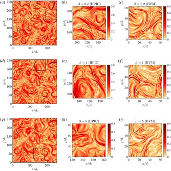
Comparison between the in-plane magnetic field modulus, $|B_{\bot }|$ , in the HPIC and the HVM simulations, for $\unicode[STIX]{x1D6FD}=0.2$ , 1 and 5 (a–c, d–f and g–i). We report the entire HPIC boxes (a,d,g) and a zoomed version of them (b,e,h), in order to match the size of the HVM boxes (c,f,i).

As a first step, we provide a qualitative picture of the fully developed turbulent dynamics arising in the two sets of simulations. A characteristic feature of turbulence in magnetized plasmas is the formation of current sheets and coherent magnetic structures, as highlighted from either the early MHD and the more recent kinetic simulations (e.g. Matthaeus & Lamkin Reference Matthaeus and Lamkin1986; Biskamp Reference Biskamp2003; Servidio et al. Reference Servidio, Dmitruk, Greco, Wan, Donato, Cassak, Shay, Carbone and Matthaeus2011, Reference Servidio, Valentini, Califano and Veltri2012; Karimabadi et al. Reference Karimabadi, Roytershteyn, Wan, Matthaeus, Daughton, Wu, Shay, Loring, Borovsky and Leonardis2013b ; Franci et al. Reference Franci, Landi, Matteini, Verdini and Hellinger2015a ; Navarro et al. Reference Navarro, Teaca, Told, Groselj, Crandall and Jenko2016; Cerri & Califano Reference Cerri and Califano2017), and recently observed also by direct measurements in the solar wind (Perri et al. Reference Perri, Goldstein, Dorelli and Sahraoui2012; Chasapis et al. Reference Chasapis, Retinò, Sahraoui, Vaivads, Khotyaintsev, Sundkvist, Greco, Sorriso-Valvo and Canu2015; Greco et al. Reference Greco, Perri, Servidio, Yordanova and Veltri2016). Also previous studies with HVM and with HPIC have focused on kinetic effects related to magnetic structures (Perrone et al. Reference Perrone, Valentini, Servidio, Dalena and Veltri2013; Valentini et al. Reference Valentini, Servidio, Perrone, Califano, Matthaeus and Veltri2014; Franci et al. Reference Franci, Hellinger, Matteini, Verdini and Landi2016a ; Valentini et al. Reference Valentini, Perrone, Stabile, Pezzi, Servidio, De Marco, Marcucci, Bruno, Lavraud and De Keyser2016). Therefore, an interesting quantity to look at is the modulus of the in-plane component of the magnetic field, i.e. $|\boldsymbol{B}_{\bot }|\equiv \sqrt{B_{x}^{2}+B_{y}^{2}}$ . In figure 1, we report the contour plots of $|\boldsymbol{B}_{\bot }|$ obtained with the HPIC and HVM simulations for the three values of the plasma $\unicode[STIX]{x1D6FD}$ , $\unicode[STIX]{x1D6FD}=0.2$ (a–c), 1 (d–f) and 5 (g–i). On the left panels we draw the entire simulation boxes of the HPIC simulations, from which a zoom is shown in the central panels in order to match the size of the HVM simulation boxes, which are instead shown on the right panels. The snapshots are taken at a given time, corresponding to the peak of the turbulent activity, $t_{peak}$ , in the HPIC simulations and to a (random) time within the quasi-steady turbulent state in the HVM runs. 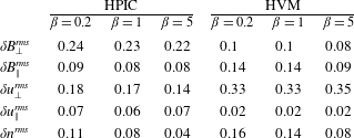Here $t_{peak}$ is defined as the time at which the root-mean-square (r.m.s.) value of the current density, $\boldsymbol{J}$ , presents a peak, thus indicating strong nonlinear (turbulent) activity (Mininni & Pouquet Reference Mininni and Pouquet2009). Note that the difference in the initial r.m.s. level of magnetic fluctuations between the two sets of simulations is quite large, i.e. a factor of 24 when comparing only their perpendicular components and of approximately 15 when also including the parallel components. While the level of fluctuations remain almost constant in the HPIC simulations (the relative decrease is less than 2 % between $t=0$ and $t_{peak}$ ), they considerably increase, of approximately an order of magnitude, in the HVM simulations. The differences in the total and perpendicular fluctuations reduce to a factor of 3 and ${\sim}1.5$ , respectively, during the quasi-steady phase. Consequently, both approaches achieve a value of the order of ${\sim}10\,\%$ of the initial background magnetic field (see table 2).

Table 2.

Root-mean-square value of the fluctuations in the developed turbulent state.

A difference is observed in the early evolution of the simulations: with respect to the time at which a fully developed turbulent state is reached, the HPIC runs start developing current sheets and small-scale magnetic structures earlier than their HVM counterparts. This different behaviour is due to the different initialization, i.e. the very different level of initial fluctuations and the very different number of modes, and to the different approach implemented for developing and sustaining the turbulent cascade (free decay versus forcing). In the HVM runs, the initial very small level of fluctuations increases due to the continuous energy injection (and the very long initial nonlinear time decreases accordingly), thus determining a smooth transition from a weak to a strong turbulence regime. On the other hand, in the HPIC simulations, the injection-scale nonlinear time at $t=0$ is already of the same order as its HVM counterpart in the quasi-steady turbulent state. As a result, in the HPIC case, many vortices and large-scale magnetic islands are suddenly generated and strong ion-scale gradients in the magnetic field (and, consequently, current sheets) quickly form between them. Despite the different early evolution, it can be noted that once the turbulent cascade is fully developed, the two sets of simulations exhibit the same qualitative behaviour for all three $\unicode[STIX]{x1D6FD}$ cases in terms of the small-scale magnetic structures. In particular, all simulations exhibit reconnection occurring around the ion scales, leading to the formation of several small-scale island-like structures and to the full development of turbulence (see, e.g. Cerri & Califano Reference Cerri and Califano2017). These features can be indeed relevant in the context of the problem of turbulent dissipation in the solar wind as, for instance, the so-called ‘turbulent dissipation challenge’ (Parashar et al. Reference Parashar, Salem, Wicks, Karimabadi, Gary and Matthaeus2015), where many observations have been focusing on the nature of magnetic fluctuations around the ion characteristic scales (see, e.g. Lion, Alexandrova & Zaslavsky Reference Lion, Alexandrova and Zaslavsky2016; Perrone et al. Reference Perrone, Alexandrova, Mangeney, Maksimovic, Lacombe, Rakoto, Kasper and Jovanovic2016; Roberts et al. Reference Roberts, Li, Alexandrova and Li2016, and references therein). Coherent structures of larger sizes are clearly visible in the HPIC simulations, whereas they are much less evident in the HVM runs. In the HPIC simulations, the strong small-scale gradients are therefore embedded in a large-scale background with comparable energy. 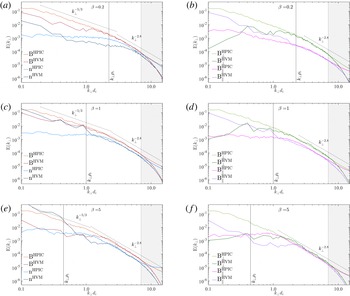In the HVM simulations, instead, such large-scale background of $B_{\bot }$ fluctuations is much less energetic and almost all the visible magnetic structures exhibit a width of the order of the ion scales. These features of the two sets of simulations determine the observed sharper shapes and a higher contrast of the HVM contours in figure 1. Such behaviour is indeed even clearer when comparing the spectra of perpendicular and parallel magnetic fluctuations (see figure 2 b,d,f): an extremely good agreement is recovered across and below the ion kinetic scales, i.e. when any possible influence of the different initial set-up and/or of the injection mechanism has faded away, whereas at the largest scales, the two set of simulations dramatically differ, since the dominant contribution of magnetic fluctuations comes from the perpendicular component in HPIC simulations and from the parallel one in HVM simulations. The behaviour of magnetic structures in real space provide a first, qualitative, evidence that, as expected, the kinetic turbulent cascade and the consequent formation of small-scale structures essentially lose memory of the initial condition and/or of the injection-versus-decay mechanism, and they are relatively independent of the dissipation mechanisms.

Figure 2.

Comparison between the results of the HPIC and the HVM approaches for the power spectra of the density, $n$ , of the magnetic field, $B$ (a,c,e), and of its perpendicular, $B_{\bot }$ , and parallel, $B_{\Vert }$ , components (b,d,f) for $\unicode[STIX]{x1D6FD}=0.2$ , 1, and 5 ((a,b), (c,d) and (e,f), respectively). The grey shaded region marks the range where the spectra are affected by numerical effects.

3.2 Spectral properties of turbulent fluctuations

We now focus our attention on the energy spectra of the turbulent fluctuations. Note that for both the HPIC and the HVM simulations we show the spectra time averaged over a time interval $\unicode[STIX]{x0394}t\simeq 15\unicode[STIX]{x1D6FA}_{ci}^{-1}$ , corresponding to nearly half of the outer-scale nonlinear time. Since the r.m.s. level of fluctuations at the injection scale and the numerical effects at the smallest scales are different for the two set of simulations, we have rescaled the spectra of all quantities by a common factor in order to compare their behaviour in the kinetic range at a given $\unicode[STIX]{x1D6FD}$ . We have chosen such a factor to be the ratio between the HVM and the HPIC total magnetic spectrum at the latest scale before which the two intrinsically different numerical effects start to kick in, i.e. $k_{\bot }d_{i}=7$ , assumed to be the inner scale (Biskamp Reference Biskamp2003). We stress that the applied shift is based only on the total magnetic spectrum, but in the kinetic range it will automatically produce overlapping spectra also for $\unicode[STIX]{x1D6FF}B_{\Vert }$ , $\unicode[STIX]{x1D6FF}B_{\bot }$ and $\unicode[STIX]{x1D6FF}n$ (see below).

In figure 2, we compare the power spectra of the density and total magnetic fluctuations, $E_{n}(k_{\bot })$ and $E_{B}(k_{\bot })$ respectively (a,c,e), and those of the parallel and perpendicular magnetic fluctuations separately, $E_{B\Vert }(k_{\bot })$ and $E_{B\bot }(k_{\bot })$ respectively (b,d,f,). The comparison is shown for the three different values of the plasma $\unicode[STIX]{x1D6FD}$ , $\unicode[STIX]{x1D6FD}=0.2$ (a,b), 1 (c,d) and 5 (e,f,). The wavenumber axis is given in $d_{i}$ units and a $\unicode[STIX]{x1D6FD}$ -dependent $k_{\bot }\unicode[STIX]{x1D70C}_{i}=1$ vertical line is displayed in the plots. The grey shaded area at $k_{\bot }d_{i}>7$ highlights the part of the spectrum that is potentially affected by numerical effects, namely when the HPIC simulations are close to the PPC noise level and when numerical filtering is significant in the HVM runs (note that this is a conservative choice, since, for instance, density and magnetic field spectra typically exhibit a power law beyond $k_{\bot }d_{i}=7$ ).

We see that the spectra are in disagreement at large scales due to the different initialization adopted by the HPIC and the HVM simulations. This is particularly evident when looking at the density spectrum, $E_{n}$ , or when comparing the parallel and perpendicular magnetic fluctuation spectra, $E_{B\Vert }$ and $E_{B\bot }$ . In fact, on the one hand, the HVM simulations drive partially compressive large-scale momentum fluctuations that develop a higher level of large-scale density and parallel magnetic fluctuations with respect to the HPIC counterparts. On the other hand, the HPIC simulations implement a higher level of large-scale perpendicular magnetic fluctuations with respect to the level reached in the HVM turbulent state at the same large scales. Nevertheless the turbulent spectra in the two cases agree more and more as the cascade goes on and energy is transferred towards smaller and smaller scales, eventually reaching a complete agreement at ion scales. In particular, as the ion kinetic scales are approached, we observe a switch in the level of the parallel and perpendicular magnetic spectra for the HVM cases, thus denoting a self-consistent ‘readjustment’ of the system at small scales (see figure 2 b,d,f). At $\unicode[STIX]{x1D6FD}=5$ , being the level of the large-scale density fluctuations larger than the magnetic counterpart in the HVM case, one finds the same behaviour, i.e. the density and magnetic fluctuation levels switch while the turbulent cascade proceeds towards small scales (figure 2 e). It is worth noticing that the agreement between the HPIC and HVM results for the high- $\unicode[STIX]{x1D6FD}$ regime is only met at $k_{\bot }\unicode[STIX]{x1D70C}_{i}\gg 1$ , since the external forcing employed in the Vlasov simulations acts very close to the ion gyroradius. Therefore, the system needs some ‘cascade time’ in order to self-consistently reprocess the turbulent fluctuations, leading to an agreement between HVM and HPIC at somewhat smaller scales than $k_{\bot }\unicode[STIX]{x1D70C}_{i}\sim 1$ . Within the kinetic range, where the HVM and HPIC spectra nearly overlap, one can compute the slopes as the average between the two spectra. With this method, the spectral slopes for the total, parallel and perpendicular magnetic fluctuations turn out to be $\unicode[STIX]{x1D6FC}_{B}\simeq -2.85$ , $\unicode[STIX]{x1D6FC}_{B\Vert }\simeq -2.8$ and $\unicode[STIX]{x1D6FC}_{B\bot }\simeq -2.9$ , respectively, for $\unicode[STIX]{x1D6FD}=1$ . Analogously, at $\unicode[STIX]{x1D6FD}=0.2$ and $\unicode[STIX]{x1D6FD}=5$ , the corresponding spectral slopes are instead $\unicode[STIX]{x1D6FC}_{B}\simeq -3$ , $\unicode[STIX]{x1D6FC}_{B\Vert }\simeq -2.6$ , $\unicode[STIX]{x1D6FC}_{B\bot }\simeq -3.1$ , and $\unicode[STIX]{x1D6FC}_{B}\simeq -2.9$ , $\unicode[STIX]{x1D6FC}_{B\Vert }\simeq -2.75$ , $\unicode[STIX]{x1D6FC}_{B\bot }\simeq -2.9$ , respectively. The density fluctuations, for those cases where a power law can be identified, always set up a kinetic spectrum with a slope consistent with $\unicode[STIX]{x1D6FC}_{n}\approx -2.8$ . These trends are consistent with the results presented in Franci et al. (Reference Franci, Landi, Matteini, Verdini and Hellinger2016b ), where an accurate fitting procedure was employed and for a wider $\unicode[STIX]{x1D6FD}$ range.

Figure 3.

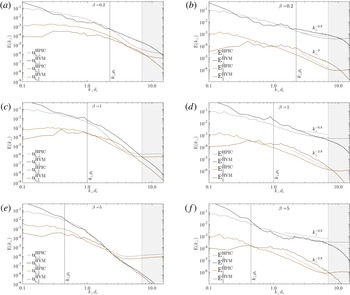
The same as in figure 2, but for the power spectra of the perpendicular, $u_{i,\bot }$ , and parallel, $u_{i,\Vert }$ , components of the ion bulk velocity (a,c,e) and of the perpendicular, $E_{\bot }$ , and parallel, $E_{\Vert }$ , components of the electric field (b,d,f,).

Let us now focus our attention on the velocity and electric fluctuation spectra. These quantities are particularly sensitive to this comparison for two different reasons: first, the numerical treatment of the velocity space represents the main difference between HVM and HPIC, and, second, the electric field is a derived quantity and thus possibly more affected by the different numerical effects which are present in both codes. In figure 3, similarly to figure 2, we now compare the power spectra of the parallel and perpendicular velocity fluctuations, $E_{u\Vert }(k_{\bot })$ and $E_{u\bot }(k_{\bot })$ , respectively (a,c,e), and the power spectra of the parallel and perpendicular electric fluctuations, $E_{E\Vert }(k_{\bot })$ and $E_{E\bot }(k_{\bot })$ , respectively (b,d,f). Velocity fluctuations do indeed exhibit a significant disagreement between HPIC and HVM. In particular, at $\unicode[STIX]{x1D6FD}=0.2$ and $\unicode[STIX]{x1D6FD}=1$ , it seems that the HVM spectra maintain a clear power law at smaller scales (before numerical damping starts to be effective, as indicated by the grey shaded area), while their HPIC counterparts are damped as the ion gyroradius scale is crossed, until a plateau is observed as the PPC noise level is reached. For $\unicode[STIX]{x1D6FD}=5$ , instead, velocity spectra are steepening roughly in the same way at $k_{\bot }\unicode[STIX]{x1D70C}_{i}>1$ , and thus a better agreement between the two methods is found. The different small-scale behaviours of the velocity spectra for $\unicode[STIX]{x1D6FD}\leqslant 1$ does not seem to be a consequence of the different approach (HPIC versus HVM), but rather of the different injection method (free decay versus forcing). In this respect, it is worth mentioning that what is observed in the present HPIC simulations is rather comparable to what has been shown by previous HVM simulations of freely decaying turbulence in Servidio et al. (Reference Servidio, Valentini, Perrone, Greco, Califano, Matthaeus and Veltri2015). In fact, by looking at three cases with similar $\unicode[STIX]{x1D6FD}$ values in Servidio et al. (Reference Servidio, Valentini, Perrone, Greco, Califano, Matthaeus and Veltri2015, figure 4), we see that the velocity spectra exhibit a very similar damping, occurring at more or less the same scales. Therefore, the reason of such difference between the HPIC velocity spectra and the HVM counterparts presented here is more likely due to a continuous injection of momentum in the HVM cases, which may be in general responsible for sustaining the cascade of velocity fluctuations (cf. also table 2). Finally, due to the quick drop of the HPIC velocity spectra at small scales, the PPC noise level is reached slightly before $k_{\bot }d_{i}\sim 7$ . However note that the $y$ -range used for these spectra is larger with respect to the one used for the other spectra and thus, since their power is several orders of magnitude below the other fields, we do not expect that these features play a fundamental role in the other spectra (see figure 2) and in the Ohm’s law at the kinetic scale, where the MHD term related to $\boldsymbol{u}$ is by definition negligible. Also, concerning the perpendicular and the parallel components of the electric field fluctuations, although $\boldsymbol{E}$ is a derived field (and thus more sensitive to numerics and noise due, e.g. to the density gradient), we do observe a reasonable level of agreement between the HVM and the HPIC power spectra. In this regard, since $\boldsymbol{E}$ is computed through the generalized Ohm’s law, it is possible to recover a prediction for its slope in the kinetic range by considering the contributions from its terms separately, as previously done in Franci et al. (Reference Franci, Verdini, Matteini, Landi and Hellinger2015b ). The main contributions at sub-ion scales come from the Hall term, $\boldsymbol{E}^{Hall}$ , and the electron pressure gradient term, $\boldsymbol{E}^{pe}$ , since the steepening of the velocity spectra makes the MHD term, $\boldsymbol{E}^{MHD}$ , negligible. The leading terms of the perpendicular and of the parallel electric field at sub-ion scales are given by

respectively. Consequently, the expected slope can be recovered as Since the slope of $E_{B_{\Vert }}$ and $E_{B_{n}}$ at sub-ion scales is ${\sim}-2.8$ for all three $\unicode[STIX]{x1D6FD}$ regimes (see figure 2), the predicted slope of $E_{E_{\bot }}$ is $-0.8$ in all cases. On the contrary, the slope of $E_{B_{\bot }}$ slightly changes with $\unicode[STIX]{x1D6FD}$ , being close to $-3.2$ for $\unicode[STIX]{x1D6FD}=0.2$ , $-3$ for $\unicode[STIX]{x1D6FD}=1$ and $-3$ for $\unicode[STIX]{x1D6FD}=5$ (figure 2 b,d,f). Therefore, the slope of $E_{E\Vert }$ is expected to be close to $-3.0$ for $\unicode[STIX]{x1D6FD}=0.2$ , $-2.8$ for $\unicode[STIX]{x1D6FD}=1$ and $-2.8$ for $\unicode[STIX]{x1D6FD}=5$ . A very good agreement is observed between the results of all simulations and these theoretical predictions for both the perpendicular and the parallel electric spectra and for all three values of $\unicode[STIX]{x1D6FD}$ , up to $k_{\bot }d_{i}\sim 7$ , where the HPIC spectra flattens due to numerical noise while the HVM spectra drops due to filtering. The only difference is observed in the spectrum of the perpendicular electric field for $\unicode[STIX]{x1D6FD}=1$ , since the velocity spectra of the HPIC and of the HVM runs start differing at $k_{\bot }d_{i}\gtrsim 1$ . The larger level of fluctuations in the HVM case thus provides a non-negligible contribution of the MHD term, $\boldsymbol{E}_{\bot }^{MHD}\propto \boldsymbol{u}_{\bot }\times \boldsymbol{B}_{0}$ , at those scales, which makes $E_{E_{\bot }}$ be a little steeper around the ion scales.

3.3 Relation between density and parallel magnetic fluctuations

By looking at the expected relation between the density and parallel magnetic fluctuations for kinetic Alfvén wave (KAW) fluctuations, it was recently shown in Cerri et al. (Reference Cerri, Califano, Jenko, Told and Rincon2016) that turbulence properties in driven 2D-3V HVM simulations were undergoing to a transition when passing from a $\unicode[STIX]{x1D6FD}\geqslant 1$ to a low- $\unicode[STIX]{x1D6FD}$ regime. In particular, at $\unicode[STIX]{x1D6FD}\geqslant 1$ , it was found that $\unicode[STIX]{x1D6FF}n$ and $\unicode[STIX]{x1D6FF}B_{\Vert }$ fluctuations were satisfying the relation expected for KAW turbulence, whereas that was not the case for the low- $\unicode[STIX]{x1D6FD}$ regime. Here, we consider again this aspect of the small-scale turbulent fluctuations and we compare the HVM results with the HPIC simulations of freely decaying large-scale Alfvénic fluctuations. The aim of this further comparison is to understand whether this transition depends on the particular choice of the injection mechanism and on the nature of the large-scale fluctuations feeding the cascade, or if there is a self-consistent reprocessing of the large-scale turbulent fluctuations realized by the system as soon as the cascade crosses the ion kinetic scales.

Figure 4.

Comparison between the HPIC and the HVM spectra of the parallel magnetic fluctuations, $E_{B_{\Vert }}$ (solid lines), and of the normalized density fluctuations, $E_{\widetilde{n}}$ (dashed lines), along with their ratio, $E_{B_{\Vert }}/E_{\widetilde{n}}$ , at the bottom of each panel, for $\unicode[STIX]{x1D6FD}=0.2$ , 1 and 5 (a,b,c, respectively). The grey shaded region marks the range where the spectra are affected by numerical effects.

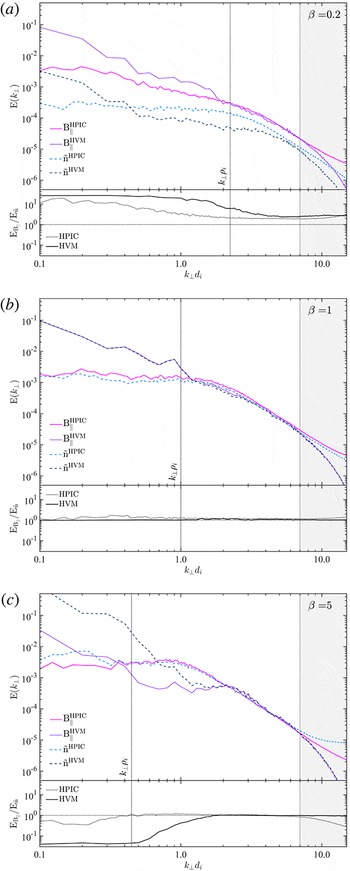
In figure 4 we show a comparison between the HPIC and the HVM spectrum of the parallel magnetic fluctuations and of the normalized density fluctuations, $E_{B_{\Vert }}$ (solid lines) and $E_{\widetilde{n}}$ (dashed lines), along with their ratio at the bottom of each panel, for the three different plasma $\unicode[STIX]{x1D6FD}$ parameters, namely $\unicode[STIX]{x1D6FD}=0.2$ , 1 and 5 (a,b,c, respectively). Here, the density fluctuations are normalized accordingly with the relation between the density and the parallel magnetic fluctuations that is expected for kinetic Alfvén waves (Schekochihin et al. Reference Schekochihin, Cowley, Dorland, Hammett, Howes, Quataert and Tatsuno2009; Boldyrev et al. Reference Boldyrev, Horaites, Xia and Perez2013; Chen et al. Reference Chen, Boldyrev, Xia and Perez2013),

where $\unicode[STIX]{x1D70F}$ is the electron-to-proton temperature ratio and it is set to unity for all simulations (the normalization parameter is therefore a function of the plasma $\unicode[STIX]{x1D6FD}$ parameter only). With such normalization, the prediction for KAW fluctuations would then be $\unicode[STIX]{x1D6FF}B_{\Vert }=\unicode[STIX]{x1D6FF}\widetilde{n}$ , so a ratio $E_{B_{\Vert }}/E_{\unicode[STIX]{x1D6FF}\widetilde{n}}$ equal, or very close, to unity would indicate that the main contribution to small-scale turbulence is given by KAW-like fluctuations. Such transition to a KAW scenario is supposed to take place at the ion gyro-scale. On the contrary, when deviations from unity are significant, it would denote a case in which KAW fluctuations can only be a sub-dominant contribution to small-scale turbulence. From figure 4, we can thus conclude that the $\unicode[STIX]{x1D6FD}=1$ case (b) is somehow the most Alfvénic case, since such ratio is always very close to unity, both at large and at small scales. At $\unicode[STIX]{x1D6FD}=5$ , there is instead a clear transition to KAW turbulence as soon as the ion kinetic scales are crossed. Note that the scale at which this transition occurs can be affected by the injection, if this takes place at scales too close to the ion gyroradius, since, as already discussed, the system needs to accomplish a self-consistent reprocessing of the large-scale turbulent fluctuations at small scales. Nevertheless, even if such scale separation is not completely fulfilled, a transition will anyway take place at a certain scale, smaller than the expected one. This is clearly the case of the HVM simulation with $\unicode[STIX]{x1D6FD}=5$ . On the contrary, in the HPIC run with the same value of $\unicode[STIX]{x1D6FD}$ , the transition is observed around $k_{\bot }\unicode[STIX]{x1D70C}_{i}\sim 1$ , as expected. In this case, the initial injection scale is the same as for the HVM case, i.e. $k_{\bot }d_{i}\sim 0.3$ . However, due to the free decay, by the time at which the quasi-steady turbulent state is reached that scale has been fully involved in the cascade and thus the effective injection scale has been ‘shifted’ towards larger scales, $k_{\bot }d_{i}\lesssim 0.1$ , i.e. sufficiently far from the ion gyro-scale. The fact that both the HVM and the HPIC simulations, despite this difference, still reach the same ratio at small scales, can be interpreted as a further evidence for the self-consistent response of the plasma system in a defined regime. A different result is found instead for $\unicode[STIX]{x1D6FD}=0.2$ , where the ratio $E_{B_{\Vert }}/E_{\widetilde{n}}$ is significantly different from unity in both cases, although the injection is well separated from the ion scales in this $\unicode[STIX]{x1D6FD}$ regime. In particular, a clear and extended plateau at a value $E_{B_{\Vert }}/E_{\unicode[STIX]{x1D6FF}\widetilde{n}}\sim 3$ is observed at small scales, starting from $k_{\bot }\unicode[STIX]{x1D70C}_{i}\sim 1$ in the HPIC case and from slightly larger scales in the HVM case. Such deviation is indeed significant and it thus denotes a sub-dominant contribution of KAWs fluctuations to small-scale turbulence. It is worth stressing that, despite the existence of some indications about the presence of magnetosonic/whistler fluctuations in this low- $\unicode[STIX]{x1D6FD}$ regime, other kinds of fluctuations cannot be excluded a priori. Therefore we remind the reader that proving that KAWs are subdominant does not automatically select magnetosonic/whistler fluctuations as the dominant contribution.