2.1 Dimensional model: general equations – rheology

We consider an incompressible, purely viscous fluid. Its Eulerian velocity field $\boldsymbol{v}$ therefore fulfils

(2.1) $$\begin{eqnarray}\displaystyle \text{div}\boldsymbol{v}=0. & & \displaystyle\end{eqnarray}$$

It evolves according to the linear momentum equation

(2.2) $$\begin{eqnarray}\displaystyle \unicode[STIX]{x1D70C}[\unicode[STIX]{x2202}_{t}\boldsymbol{v}+(\unicode[STIX]{x1D735}\boldsymbol{v})\boldsymbol{\cdot }\boldsymbol{v}]=-\unicode[STIX]{x1D735}p+\boldsymbol{d}\boldsymbol{i}\boldsymbol{v}(\unicode[STIX]{x1D64F}), & & \displaystyle\end{eqnarray}$$

with $\unicode[STIX]{x1D70C}$ the fluid density, $p$ a generalized pressure, which includes the effect of the gravity force, $\unicode[STIX]{x1D64F}$ the viscous stress tensor. This tensor

(2.3) $$\begin{eqnarray}\displaystyle \unicode[STIX]{x1D64F}=\unicode[STIX]{x1D702}\,\unicode[STIX]{x1D63F}, & & \displaystyle\end{eqnarray}$$

with $\unicode[STIX]{x1D702}$ the dynamic viscosity and

(2.4) $$\begin{eqnarray}\displaystyle \unicode[STIX]{x1D63F}=\unicode[STIX]{x1D735}\boldsymbol{v}+(\unicode[STIX]{x1D735}\boldsymbol{v})^{\text{T}} & & \displaystyle\end{eqnarray}$$

the rate-of-strain tensor. The second invariant of this tensor,

(2.5) $$\begin{eqnarray}\displaystyle \unicode[STIX]{x1D6E4}_{2}={\textstyle \frac{1}{2}}\unicode[STIX]{x1D63F}\boldsymbol{ : }\unicode[STIX]{x1D63F}={\textstyle \frac{1}{2}}\unicode[STIX]{x1D60B}_{ij}\unicode[STIX]{x1D60B}_{ij}, & & \displaystyle\end{eqnarray}$$

the ‘rate-of-strain intensity’, equals the square of the shear rate $\dot{\unicode[STIX]{x1D6FE}}$ in viscometric flows. The Carreau’s law reads

(2.6) $$\begin{eqnarray}\displaystyle \unicode[STIX]{x1D702}=\unicode[STIX]{x1D702}(\unicode[STIX]{x1D6E4}_{2})=\unicode[STIX]{x1D702}_{\infty }+(\unicode[STIX]{x1D702}_{0}-\unicode[STIX]{x1D702}_{\infty })(1+\unicode[STIX]{x1D706}_{C}^{2}\unicode[STIX]{x1D6E4}_{2})^{(n_{C}-1)/2}. & & \displaystyle\end{eqnarray}$$

The corresponding flow curves are usually presented as log–log graphs of $\unicode[STIX]{x1D702}$ versus $\dot{\unicode[STIX]{x1D6FE}}=\sqrt{\unicode[STIX]{x1D6E4}_{2}}$ (figure 1 $a$ , see also the figure 14 of Draad et al. Reference Draad, Kuiken and Nieuwstadt1998). They present three regions:

1. (i) at low shear rate $\dot{\unicode[STIX]{x1D6FE}}<\unicode[STIX]{x1D706}_{C}^{-1}$ a plateau with the ‘Newtonian viscosity’ $\unicode[STIX]{x1D702}_{0}$ ;

2. (ii) at intermediate shear rate, a region where the viscosity decreases with $\dot{\unicode[STIX]{x1D6FE}}$ , i.e. the shear-thinning effects occur;

3. (iii) at large shear rate $\dot{\unicode[STIX]{x1D6FE}}\gg \unicode[STIX]{x1D706}_{C}^{-1}$ , a plateau with the infinite-shear-rate viscosity $\unicode[STIX]{x1D702}_{\infty }$ .

For fluids that are not close to the Newtonian limit, for instance rather concentrated polymer solutions, the viscosity $\unicode[STIX]{x1D702}_{\infty }$ is significantly smaller than $\unicode[STIX]{x1D702}_{0}$ (Bird et al. Reference Bird, Armstrong and Hassager1987). For instance, the flow curves of figure 1 corresponds to $\unicode[STIX]{x1D702}_{0}=1130\unicode[STIX]{x1D702}_{\infty }$ ; the four flow curves of the figure 14 of Draad et al. (Reference Draad, Kuiken and Nieuwstadt1998) correspond to a value of $\unicode[STIX]{x1D702}_{0}$ which is, at least, 8 times $\unicode[STIX]{x1D702}_{\infty }$ . Since our interest is to focus on strongly non-Newtonian fluids, we will always assume that

(2.7) $$\begin{eqnarray}\displaystyle \unicode[STIX]{x1D702}_{\infty }=0, & & \displaystyle\end{eqnarray}$$

which leaves only three dimensional rheological parameters: $\unicode[STIX]{x1D702}_{0},~\unicode[STIX]{x1D706}_{C}$ and $n_{C}$ . The zero-shear-rate viscosity $\unicode[STIX]{x1D702}_{0}$ is typically of the order of, at least, $100$ times the viscosity of water. The characteristic time of the fluid $\unicode[STIX]{x1D706}_{C}$ is typically of the order of seconds or tens of seconds. The shear-thinning index $n_{C}$ varies in the range $]0,1[$ , depending on the fluid. The limit value $n_{C}=1$ corresponds to a Newtonian fluid. The smaller $n_{C}$ , the stronger the shear-thinning effects. Since $n_{C}\in ]0,1[$ , the shear stress in viscometric flows

(2.8) $$\begin{eqnarray}\displaystyle \unicode[STIX]{x1D70F}=\unicode[STIX]{x1D70F}(\dot{\unicode[STIX]{x1D6FE}})=\unicode[STIX]{x1D702}(\dot{\unicode[STIX]{x1D6FE}}^{2})\,\dot{\unicode[STIX]{x1D6FE}} & & \displaystyle\end{eqnarray}$$

is an increasing bijective function of the shear rate $\dot{\unicode[STIX]{x1D6FE}}$ (figure 1 b), whereas the viscosity $\unicode[STIX]{x1D702}$ can be considered as a decreasing bijective function of $\dot{\unicode[STIX]{x1D6FE}}$ . Consequently, in viscometric flows, one can define bijective functions $\dot{\unicode[STIX]{x1D6FE}}=\dot{\unicode[STIX]{x1D6FE}}_{v}(\unicode[STIX]{x1D70F})$ and

(2.9) $$\begin{eqnarray}\displaystyle \unicode[STIX]{x1D702}=\unicode[STIX]{x1D702}_{v}(\unicode[STIX]{x1D70F})=\unicode[STIX]{x1D702}[\dot{\unicode[STIX]{x1D6FE}}_{v}^{2}(\unicode[STIX]{x1D70F})]. & & \displaystyle\end{eqnarray}$$

2.2 Driving pressure gradient – laminar or wave flow fields

The flows are driven by a uniform pressure gradient $G_{0}$ in the axial direction, i.e.

(2.10) $$\begin{eqnarray}\displaystyle p=p_{0}-G_{0}z+\widetilde{p}, & & \displaystyle\end{eqnarray}$$

where, for the laminar flows, $\widetilde{p}$ vanishes, whereas, for the wave flows,

(2.11) $$\begin{eqnarray}\displaystyle \widetilde{p}=\mathop{\sum }_{l=-L}^{L}\mathop{\sum }_{m=-M}^{M}p_{lm}(r)\exp \{\text{i}[mm_{0}\unicode[STIX]{x1D703}+lq(z-ct)]\}. & & \displaystyle\end{eqnarray}$$

In this spectral development, $L$ and $M$ are the order of truncations of the Fourier series in $z-ct$ and $\unicode[STIX]{x1D703}$ , which are always finite in practical computations. Accordingly, the velocity field

(2.12) $$\begin{eqnarray}\displaystyle \boldsymbol{v}=u\boldsymbol{e}_{r}+v\boldsymbol{e}_{\unicode[STIX]{x1D703}}+(W_{b}+w)\boldsymbol{e}_{z}, & & \displaystyle\end{eqnarray}$$

with $W_{b}=W_{b}(r)$ the axial velocity of the laminar base flow, $u,v$ and $w$ the wave fields, which are all written as spectral expansions of the form (2.11).

2.3 Wall shear stress and wall viscosity

A global momentum balance in laminar or wave flows, in a fluid domain of length $L_{z}$ in the axial direction (see (1.5)), shows a balance between the mean wall shear stress $\unicode[STIX]{x1D70F}_{w}=-\langle T_{rz}(r=a,\unicode[STIX]{x1D703},z)\rangle _{\unicode[STIX]{x1D703}z}$ , averaged with respect to $\unicode[STIX]{x1D703}$ and $z$ , as denoted by the angular brackets, and the pressure difference between the inlet and outlet of the domain:

(2.13) $$\begin{eqnarray}\displaystyle \unicode[STIX]{x1D70F}_{w}=G_{0}a/2. & & \displaystyle\end{eqnarray}$$

One defines the dynamic wall viscosity as

(2.14) $$\begin{eqnarray}\displaystyle \unicode[STIX]{x1D702}_{w}=\unicode[STIX]{x1D702}_{v}(\unicode[STIX]{x1D70F}_{w})=\unicode[STIX]{x1D702}_{v}(G_{0}a/2), & & \displaystyle\end{eqnarray}$$

using the viscometric function (2.9). In the case of the laminar base flow, which is indeed viscometric, $\unicode[STIX]{x1D702}_{w}$ is the value of the viscosity at the wall. In the case of a wave flow, which is not viscometric, our numerical results (figures 14 e–g) will confirm that the viscosity (2.14) is also the average value of the viscosity at the wall,

(2.15) $$\begin{eqnarray}\displaystyle \unicode[STIX]{x1D702}_{w}=\langle \unicode[STIX]{x1D702}(r=a,\unicode[STIX]{x1D703},z)\rangle _{\unicode[STIX]{x1D703}z}, & & \displaystyle\end{eqnarray}$$

a result which was already suggested in Roland et al. (Reference Roland, Plaut and Nouar2010). The definition (2.14) is also used by experimentalists to define the wall viscosity in transitional or turbulent flows, from a measure of the pressure drop in a long pipe. Of course the kinematic wall viscosity

(2.16) $$\begin{eqnarray}\displaystyle \unicode[STIX]{x1D708}_{w}=\unicode[STIX]{x1D702}_{w}/\unicode[STIX]{x1D70C}. & & \displaystyle\end{eqnarray}$$

2.4 Dimensionless model

Using the centreline velocity $W_{0}$ of the laminar flow as the velocity scale, the radius $a$ of the pipe as the length scale, the advection time $t_{0}=a/W_{0}$ as the time scale, the zero-shear-rate viscosity $\unicode[STIX]{x1D702}_{0}$ as the dynamic viscosity scale, the product $\unicode[STIX]{x1D70C}W_{0}^{2}$ as the pressure and stress scale, we introduce two dimensionless parameters. The primary Reynolds number

(2.17) $$\begin{eqnarray}\displaystyle \mathit{Re}_{0}=W_{0}\,a/\unicode[STIX]{x1D708}_{0}, & & \displaystyle\end{eqnarray}$$

with $\unicode[STIX]{x1D708}_{0}=\unicode[STIX]{x1D702}_{0}/\unicode[STIX]{x1D70C}$ the zero-shear-rate kinematic viscosity, and the main non-Newtonian parameter

(2.18) $$\begin{eqnarray}\displaystyle \unicode[STIX]{x1D706}=\unicode[STIX]{x1D706}_{C}/t_{0}=\unicode[STIX]{x1D706}_{C}W_{0}/a. & & \displaystyle\end{eqnarray}$$

Other ‘secondary’ Reynolds numbers are defined in table 1.

From now on, all quantities are dimensionless, except $a,~G_{0},~W_{0},~\unicode[STIX]{x1D706}_{C},~\unicode[STIX]{x1D70C},~\unicode[STIX]{x1D702}_{0}$ and $\unicode[STIX]{x1D708}_{0}$ . The parameter $\unicode[STIX]{x1D706}$ appears in the dimensionless viscosity

(2.19) $$\begin{eqnarray}\displaystyle \unicode[STIX]{x1D702}=(1+\unicode[STIX]{x1D706}^{2}\unicode[STIX]{x1D6E4}_{2})^{(n_{C}-1)/2}. & & \displaystyle\end{eqnarray}$$

The primary Reynolds number appears in the dimensionless viscous stress tensor

(2.20) $$\begin{eqnarray}\displaystyle \unicode[STIX]{x1D64F}=\mathit{Re}_{0}^{-1}\,\unicode[STIX]{x1D702}\,\unicode[STIX]{x1D63F}. & & \displaystyle\end{eqnarray}$$

The dimensionless form of (2.2) is

(2.21) $$\begin{eqnarray}\displaystyle \unicode[STIX]{x2202}_{t}\boldsymbol{v}+(\unicode[STIX]{x1D735}\boldsymbol{v})\boldsymbol{\cdot }\boldsymbol{v}=-\unicode[STIX]{x1D735}p+\boldsymbol{d}\boldsymbol{i}\boldsymbol{v}(\unicode[STIX]{x1D64F}), & & \displaystyle\end{eqnarray}$$

where the pressure is of the form

(2.22) $$\begin{eqnarray}\displaystyle p=p_{0}-Gz+\widetilde{p}, & & \displaystyle\end{eqnarray}$$

with $G=G_{0}a/(\unicode[STIX]{x1D70C}W_{0}^{2})$ , see § 2.2.

Table 1.

Reynolds numbers. The reference laminar flow is the laminar flow at the same mean axial pressure gradient $G_{0}$ .

2.5 Power-law limit

The facts that the main non-Newtonian parameter

(2.23) $$\begin{eqnarray}\displaystyle \unicode[STIX]{x1D706}=\mathit{Re}_{0}\,\unicode[STIX]{x1D706}_{C}\unicode[STIX]{x1D708}_{0}/a^{2}, & & \displaystyle\end{eqnarray}$$

and that, at the wave onset, $\mathit{Re}_{0}$ is of the order of $10^{3}$ , suggest typical values

(2.24) $$\begin{eqnarray}\displaystyle \unicode[STIX]{x1D706}\simeq 10^{3}~1~\text{s}~500~10^{-6}~\text{m}^{2}/\text{s}/(1~\text{cm})^{2}\simeq 5000 & & \displaystyle\end{eqnarray}$$

for a pipe of diameter 2 cm. The limit $\unicode[STIX]{x1D706}\rightarrow +\infty$ is therefore relevant for the study of the wave onset. In this limit, as soon as $\unicode[STIX]{x1D6E4}_{2}>0$ , one recovers the rheological power law

(2.25) $$\begin{eqnarray}\displaystyle \unicode[STIX]{x1D702}\simeq \unicode[STIX]{x1D702}_{pl}=\unicode[STIX]{x1D706}^{n_{C}-1}\,\unicode[STIX]{x1D6E4}_{2}^{(n_{C}-1)/2}. & & \displaystyle\end{eqnarray}$$

3.1 General case

The laminar base flows correspond to $p=p_{b}=p_{0}-Gz$ and $\boldsymbol{v}=W_{b}(r)\boldsymbol{e}_{z}$ . This yields $\unicode[STIX]{x1D6E4}_{2}=(W_{b}^{\prime }(r))^{2}$ and the viscosity

(3.1) $$\begin{eqnarray}\displaystyle \unicode[STIX]{x1D702}=\unicode[STIX]{x1D702}_{b}=[1+\unicode[STIX]{x1D706}^{2}(W_{b}^{\prime }(r))^{2}]^{(n_{C}-1)/2}. & & \displaystyle\end{eqnarray}$$

The equation (2.21) therefore gives the ordinary differential equation

(3.2) $$\begin{eqnarray}\displaystyle \unicode[STIX]{x1D6FC}:=\mathit{Re}_{0}\,G=-\frac{1}{r}\frac{\text{d}}{\text{d}r}[r\,\unicode[STIX]{x1D702}_{b}\,W_{b}^{\prime }(r)]. & & \displaystyle\end{eqnarray}$$

The boundary condition dictated by the choice of the velocity unit,

(3.3) $$\begin{eqnarray}\displaystyle W_{b}(0)=1, & & \displaystyle\end{eqnarray}$$

and the no-slip condition at the pipe wall,

(3.4) $$\begin{eqnarray}\displaystyle W_{b}(1)=0, & & \displaystyle\end{eqnarray}$$

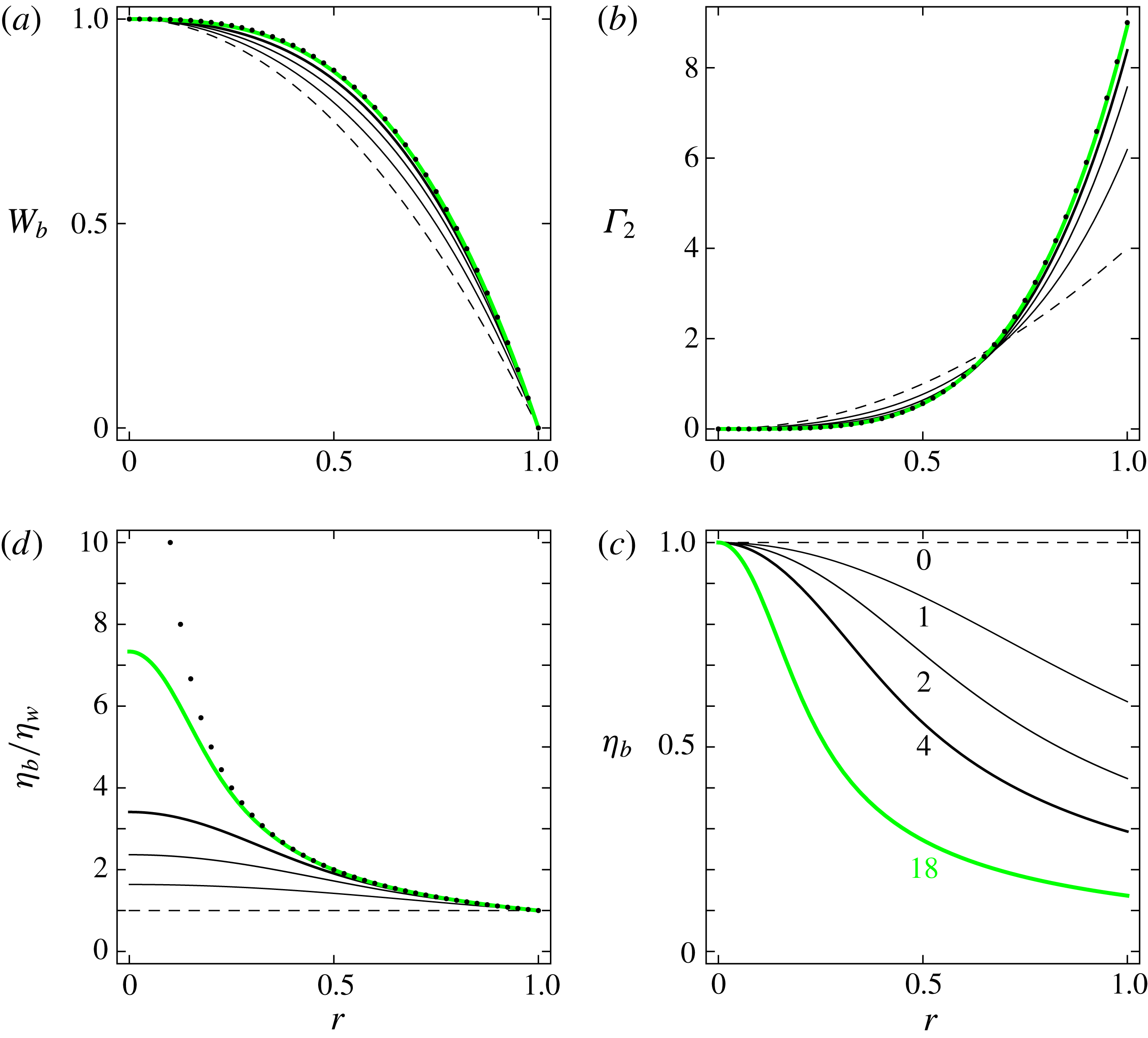
can be fulfilled only if $\unicode[STIX]{x1D6FC}$ assumes a particular value. This nonlinear boundary value problem is solved numerically. Typical results are shown in figure 2(a), which demonstrates that the flow profile depends on $\unicode[STIX]{x1D706}$ . Of course, it depends also on $n_{C}$ ; for a direct study of the influence of $n_{C}$ at finite $\unicode[STIX]{x1D706}$ (tendencies will be given in the next subsection in the case $\unicode[STIX]{x1D706}\rightarrow +\infty$ ), refer to López Carranza et al. (Reference López Carranza, Jenny and Nouar2012). When $\unicode[STIX]{x1D706}$ increases, the shear-thinning effects are more pronounced, and the flow departs more strongly from the Newtonian limit, the Hagen–Poiseuille flow. The rate of strain increases near the pipe wall (figure 2 b) and therefore the viscosity drops in this region (figure 2 c). Its value at the pipe wall, the wall viscosity

(3.5) $$\begin{eqnarray}\displaystyle \unicode[STIX]{x1D702}_{w}=\unicode[STIX]{x1D702}_{b}(r=1) & & \displaystyle\end{eqnarray}$$

will play an important role, as already advocated in § 2.3. Before discussing this, let us consider the power-law limit.

Figure 2.

Properties of the laminar base flows for $n_{C}=0.5$ and different values of $\unicode[STIX]{x1D706}$ as indicated below each curve of (c). (a) Axial velocity. (b) Rate-of-strain intensity. (c) Viscosity. (d) Ratio of the viscosity to the wall viscosity. In (a,b,d) the dots show the case of a power-law fluid, equations (3.7) and (3.11).

3.2 Power-law limit

If one replaces (3.1) by the power law

(3.6) $$\begin{eqnarray}\displaystyle \unicode[STIX]{x1D702}=\unicode[STIX]{x1D702}_{bpl}=\unicode[STIX]{x1D706}^{n_{C}-1}\,|W_{b}^{\prime }(r)|^{n_{C}-1}, & & \displaystyle\end{eqnarray}$$

the boundary value problem (3.2)–(3.4) can be solved analytically. The solution reads

(3.7a,b ) $$\begin{eqnarray}\displaystyle W_{bpl}(r)=1-r^{1+1/n_{C}},\quad W_{bpl}^{\prime }(r)=-(1+1/n_{C})\,r^{1/n_{C}}. & & \displaystyle\end{eqnarray}$$

The first equation denotes a velocity profile that becomes quite flat as $n_{C}\rightarrow 0^{+}$ , as shown, also, by the expression of the corresponding bulk velocity

(3.8) $$\begin{eqnarray}\displaystyle \overline{W}_{bpl}=[1+2/(1+3n_{C})]/3, & & \displaystyle\end{eqnarray}$$

which attains the maximum value of 1 for $n_{C}=0$ . Figures 2 and 3(a) show that the ‘power-law’ limit (3.7), (3.8) is attained as soon as $\unicode[STIX]{x1D706}\gtrsim 18$ for the typical value $n_{C}=0.5$ . Whereas its velocity profile (3.7a ) does not depend on $\unicode[STIX]{x1D706}$ , the viscosity profile of a power-law fluid,

(3.9) $$\begin{eqnarray}\displaystyle \unicode[STIX]{x1D702}_{bpl}=\unicode[STIX]{x1D706}^{n_{C}-1}\,(1+1/n_{C})^{n_{C}-1}\,r^{1-1/n_{C}}, & & \displaystyle\end{eqnarray}$$

does depend on $\unicode[STIX]{x1D706}$ . Since $n_{C}\in ]0,1[$ , $\unicode[STIX]{x1D702}_{bpl}\rightarrow +\infty$ as $r\rightarrow 0^{+}$ , where the rate of strain vanishes: this singularity is a well-known shortcoming of the power-law model. The wall viscosity of a power-law fluid,

(3.10) $$\begin{eqnarray}\displaystyle \unicode[STIX]{x1D702}_{wpl}=\unicode[STIX]{x1D702}_{bpl}(r=1)=\unicode[STIX]{x1D706}^{n_{C}-1}\,(1+1/n_{C})^{n_{C}-1}, & & \displaystyle\end{eqnarray}$$

can be used to define a viscosity ratio that is independent of $\unicode[STIX]{x1D706}$ ,

(3.11) $$\begin{eqnarray}\displaystyle \unicode[STIX]{x1D702}_{bpl}/\unicode[STIX]{x1D702}_{wpl}=r^{1-1/n_{C}}. & & \displaystyle\end{eqnarray}$$

Figure 2(d) shows how the Carreau fluids approach this limit, as $\unicode[STIX]{x1D706}$ increases, not too close of the pipe axis.

Figure 3.

For $n_{C}=0.5$ . (a) ●, Bulk velocity of the base flows; full line, power-law fluid bulk velocity of the base flows. (b) ●, Wall viscosity of the base flows; full line, power-law fluid wall viscosity of the base flows; ▪, bulk average mean viscosity of the base flows; dashed line, power-law fluid mean viscosity of the base flows; ▾, bulk average mean viscosity of the critical waves discussed in § 5.3.

3.3 Wall viscosity and mean viscosity

Figure 2(b) shows that, as soon as $\unicode[STIX]{x1D706}\gtrsim 4$ , the rate of strain at the wall approaches closely the rate of strain at the wall in the laminar flow of a power-law fluid. Consequently, the wall viscosity $\unicode[STIX]{x1D702}_{w}\simeq \unicode[STIX]{x1D702}_{wpl}$ . This is confirmed by figure 3(b).

Though the wall viscosity is a priori relevant, because it can be easily measured experimentally, from a theoretical point of view one may look at another viscosity that could be equally, or even more relevant, that is, the bulk average mean viscosity $\overline{\unicode[STIX]{x1D702}}_{b}$ . Its values, displayed in figure 3(b), are higher than the ones of the wall viscosity, since in the bulk the rate of strain is lower than at the wall (figure 2 b), hence, the viscosity is higher (figure 2 c,d). The power law for the viscosity (2.25) overestimates the viscosity in the bulk (figure 2 d). Hence the bulk average mean viscosity in laminar base flows of power-law fluids

(3.12) $$\begin{eqnarray}\displaystyle \overline{\unicode[STIX]{x1D702}}_{bpl}=\frac{2}{3}\frac{n_{C}}{n_{C}-1/3}\unicode[STIX]{x1D702}_{wpl}=\frac{2}{3}\unicode[STIX]{x1D706}^{n_{C}-1}\frac{n_{C}(1+1/n_{C})^{n_{C}-1}}{n_{C}-1/3} & & \displaystyle\end{eqnarray}$$

overestimates $\overline{\unicode[STIX]{x1D702}}_{b}$ , as shown in figure 3(b). The viscosity $\overline{\unicode[STIX]{x1D702}}_{bpl}$ cannot be defined for strongly shear-thinning fluids with $n_{C}\in ]0,1/3]$ . In such cases, the viscosity (3.9) diverges too rapidly as $r\rightarrow 0^{+}$ . We will not address such cases in this work, which will be restricted to shear-thinning fluids with $n_{C}\gtrsim 0.4$ .

4.1 Laminar flows

In the Newtonian case, $\unicode[STIX]{x1D6FC}=4$ , $\overline{W}=\overline{W}_{b}=1/2$ and $\unicode[STIX]{x1D702}_{w}=1$ give the well-known relation

(4.5) $$\begin{eqnarray}\displaystyle f\,\mathit{Re}=64. & & \displaystyle\end{eqnarray}$$

In the non-Newtonian case, figure 3(a) has already shown that, as $\unicode[STIX]{x1D706}$ increases, $\overline{W}_{b}$ approaches rapidly the value $\overline{W}_{bpl}$ given by (3.8) for a power-law fluid. Figure 4(a) shows that $\unicode[STIX]{x1D6FC}$ also approaches the value

(4.6) $$\begin{eqnarray}\displaystyle \unicode[STIX]{x1D6FC}_{pl}=2\,\unicode[STIX]{x1D706}^{n_{C}-1}(1+1/n_{C})^{n_{C}} & & \displaystyle\end{eqnarray}$$

corresponding to the power-law fluid. Hence, the product $f\,\mathit{Re}_{w}$ approaches the power-law fluid value

(4.7) $$\begin{eqnarray}\displaystyle f_{bpl}\,\mathit{Re}_{w}=16(3+1/n_{C}), & & \displaystyle\end{eqnarray}$$

as displayed in figure 4(b). The Newtonian case (4.5) is recovered when $n_{C}=1$ . Also, when $n_{C}$ decreases, the product $f_{bpl}\,\mathit{Re}_{w}$ increases, which indicates a larger friction in more shear-thinning fluids.

4.2 Travelling waves

The waves that will be described in § 5 correspond to sustained perturbations of a given laminar base flow at fixed $n_{C}$ and $\unicode[STIX]{x1D706}$ , fixed pressure gradient. The parameter $\unicode[STIX]{x1D6FC}$ and the wall viscosity are the ones of the laminar base flow. On the contrary, the mean velocity $\overline{W}$ is smaller in wave flows than in base flows (§ 5.3.1): this results in a decrease of $\mathit{Re}_{w}$ and an increase of $f\mathit{Re}_{w}$ , which signifies an increase of the drag. A further study, where the wave flows are compared to the laminar flows with the same bulk velocity, and the pressure gradient growth is directly quantified, is presented in § 6.

Figure 5.

For $n_{C}=0.5$ , $\unicode[STIX]{x1D706}=1$ . Onset curves of the saddle-node bifurcations Reynolds numbers $\mathit{Re}(q;n_{C},\unicode[STIX]{x1D706})$ (left ordinate axis) and $\mathit{Re}_{w}(q;n_{C},\unicode[STIX]{x1D706})$ (right ordinate axis); dashed lines, critical wavenumber and Reynolds numbers; $\star$ , solution found by Roland et al. (Reference Roland, Plaut and Nouar2010).

5.1 Principles of the computations of the waves and onset curves

The specific pseudospectral code used for the computations of the waves has been described and validated in Roland et al. (Reference Roland, Plaut and Nouar2010). It is pointed out that the shift-and-reflect symmetry (1.6) is fulfilled by construction, and that a phase condition is chosen, equation (46) of Roland et al. (Reference Roland, Plaut and Nouar2010). It fixes the azimuthal position of the rolls, as it will be visible in the figure 10. Computations are done at fixed rheological parameters $n_{C}$ and $\unicode[STIX]{x1D706}$ , fixed pressure gradient $G$ , i.e. fixed primary Reynolds number $\mathit{Re}_{0}$ and fixed axial wavenumber $q$ . Once a wave is obtained, its phase velocity $c$ , bulk velocity $\overline{W}$ , Reynolds numbers $\mathit{Re}$ , $\mathit{Re}_{w}$ , are output of the computations. Continuation is used to vary $n_{C}$ , $\unicode[STIX]{x1D706}$ , the Reynolds numbers or the axial wavenumber $q$ . The novelty here is a systematic study of the influence of $q$ on the EFKW waves $m_{0}=3$ that appear, through saddle-node bifurcations, at low $\mathit{Re}$ or $\mathit{Re}_{w}$ , whereas, in Roland et al. (Reference Roland, Plaut and Nouar2010), we used $q=q_{cN}=2.44$ . The Reynolds number of these saddle-node bifurcations are denoted

(5.1a,b ) $$\begin{eqnarray}\displaystyle \mathit{Re}(q;n_{C},\unicode[STIX]{x1D706})\quad \text{or}\quad \mathit{Re}_{w}(q;n_{C},\unicode[STIX]{x1D706}), & & \displaystyle\end{eqnarray}$$

which define ‘onset curves’, see figure 5. Since, for fixed rheological parameters $n_{C}$ and $\unicode[STIX]{x1D706}$ , the wall viscosity $\unicode[STIX]{x1D702}_{w}$ is uniquely determined as explained in § 2.3, $\unicode[STIX]{x1D702}_{w}=\unicode[STIX]{x1D702}_{w}(n_{C},\unicode[STIX]{x1D706})$ the viscosity at the wall in the laminar base flow, one has

(5.2) $$\begin{eqnarray}\displaystyle \mathit{Re}_{w}(q;n_{C},\unicode[STIX]{x1D706})=\mathit{Re}(q;n_{C},\unicode[STIX]{x1D706})/\unicode[STIX]{x1D702}_{w}(n_{C},\unicode[STIX]{x1D706}). & & \displaystyle\end{eqnarray}$$

Therefore the waves that appear at low $\mathit{Re}_{w}$ are identical to the ones that appear at low $\mathit{Re}$ . The focus is on these waves, that we follow with continuation methods, starting from the Newtonian EFKW waves, $\unicode[STIX]{x1D706}=0$ , and progressively increasing $\unicode[STIX]{x1D706}$ at fixed $n_{C}$ . As compared with Roland et al. (Reference Roland, Plaut and Nouar2010), we have improved the determination of the saddle-node bifurcation points by fitting, close to the bifurcation point, curves of $\mathit{Re}$ versus $c$ , the phase velocity (curves like the ones visible in figure 6), and of $\mathit{Re}$ versus $\overline{W}$ , the bulk velocity, with polynomials of degree 2 in $\mathit{Re}$ , and extracting the minima of these polynomials. Also, the optimization of $q$ has led to lower values of the Reynolds numbers. Therefore, the computations have converged, as far as global quantities are concerned ( $c,\overline{W},\ldots$ ), for all values of $n_{C}$ and $\unicode[STIX]{x1D706}$ studied here, $0.5\leqslant n_{C}\leqslant 1$ , $0\leqslant \unicode[STIX]{x1D706}\leqslant 18$ , with truncation parameters $N_{r}=28$ , $M=10$ , $L=7$ with the notations of Roland et al. (Reference Roland, Plaut and Nouar2010). The number of spectral modes is therefore $N_{r}(2M+1)(2L+1)=8820$ . However, to obtain a good description of the velocity and viscosity fields in the whole pipe (e.g. for figure 14), higher numbers of modes have been used for the strongly shear-thinning fluids, $N_{r}\simeq 40$ , $M\simeq 12$ , $L\simeq 9$ .

Figure 6.

For $n_{C}=0.5$ , $\unicode[STIX]{x1D706}=2$ . Black curves: three branches of wave solutions for $q=2.28$ : thick line, lower branch; thin continuous line, intermediate branch; thin dashed line, higher branch. Grey (green online) curve: lower branch of wave solutions for $q=2.32$ .

5.2 Onset curves – definition of the critical waves

For $n_{C}=0.5$ , $\unicode[STIX]{x1D706}=1$ , i.e. a weakly shear-thinning fluid, the onset curves obtained are shown in figure 5. The rightmost and upmost point in these curves corresponds to $q=q_{cN}$ , $\mathit{Re}_{w}(q_{cN};0.5,1)=2028$ , to be compared to the Newtonian value $\mathit{Re}_{w}(q_{cN};0.5,0)=1251$ , see (1.2). This indicates a strong stabilization of the EFKW waves, which was already evidenced in Roland et al. (Reference Roland, Plaut and Nouar2010). Importantly, when the wavenumber $q$ is decreased, the waves appear at lower values of the Reynolds numbers, until a ‘critical’ value $q_{c}$ of $q$ is attained, $q_{c}=q_{c}(n_{C},\unicode[STIX]{x1D706})$ , corresponding to ‘critical’ minimal values of the Reynolds numbers $\mathit{Re}_{c}(n_{C},\unicode[STIX]{x1D706})=\mathit{Re}(q_{c};n_{C},\unicode[STIX]{x1D706})$ ; $\mathit{Re}_{wc}(n_{C},\unicode[STIX]{x1D706})=\mathit{Re}_{w}(q_{c};n_{C},\unicode[STIX]{x1D706})$ . When $q$ is further decreased, the Reynolds numbers increase. The critical parameters here are

(5.3a-c ) $$\begin{eqnarray}\displaystyle q_{c}(0.5,1)=2.23,\quad \mathit{Re}_{c}(0.5,1)=1120,\quad \mathit{Re}_{wc}(0.5,1)=1840. & & \displaystyle\end{eqnarray}$$

We name the corresponding wave solution the ‘critical’ wave solution.

In fact, several branches of solutions exist and are in competition. This was already shown by Wedin & Kerswell (Reference Wedin and Kerswell2004) in their figure 23, which displays, for $m_{0}=3,q=q_{cN}$ , three solution branches in the plane $(\mathit{Re},c)$ . We have also found multiple solution branches in the non-Newtonian cases. This is not shown in figure 5, where, quite probably, only the branch corresponding to the lowest Reynolds numbers (‘lower branch’ or ‘critical branch’) is displayed, but we now illustrate this issue by using a larger value of $\unicode[STIX]{x1D706}$ , $\unicode[STIX]{x1D706}=2$ .

For $n_{C}=0.5$ , $\unicode[STIX]{x1D706}=2$ , and an axial wavenumber $q=2.28$ , three branches of wave solutions are displayed in figure 6, which shows some similarities with the figure 23 of Wedin & Kerswell (Reference Wedin and Kerswell2004). The lower branch has been obtained by continuation from the branch corresponding to the critical point of figure 5. It is remarkable that this lower branch forms a closed loop, and that the corresponding solutions disappear in another saddle-node bifurcation at ‘large’ Reynolds numbers. The loop corresponding to this lower branch shrinks when $q$ increases, as shown in figure 6 for $q=2.32$ . When $q\simeq 2.33$ , this branch of solution disappears in a saddle-node bifurcation, with $q$ the bifurcation parameter. Therefore, the onset curves corresponding to this branch stop at $q\simeq 2.33$ , as displayed in figure 7. This branch is the ‘critical’ one; in figure 7 one can read the critical parameters

(5.4a-c ) $$\begin{eqnarray}\displaystyle q_{c}(0.5,2)=2.11,\quad \mathit{Re}_{c}(0.5,2)=973,\quad \mathit{Re}_{wc}(0.5,2)=2300. & & \displaystyle\end{eqnarray}$$

Other complicated bifurcation scenarii happen with the other branches. For instance, the solution branches computed by Roland et al. (Reference Roland, Plaut and Nouar2010) for $q=q_{cN}=2.44$ , which correspond to the stars in figures 5 and 7, are connected (respectively disconnected) to the critical wave at $\unicode[STIX]{x1D706}=1$ (respectively 2).

Figure 7.

For $n_{C}=0.5$ , $\unicode[STIX]{x1D706}=2$ . Saddle-node bifurcations Reynolds numbers $\mathit{Re}$ (left ordinate axis) and $\mathit{Re}_{w}$ (right ordinate axis) where different wave branches as shown in figure 6 appear; $\star$ , solution found by Roland et al. (Reference Roland, Plaut and Nouar2010).

Instead of elucidating these complicated and bushy bifurcation scenarii, which would be a formidable task, we choose to focus hereafter on a family of waves that we can follow as smooth functions of the rheological parameters $n_{C}$ and $\unicode[STIX]{x1D706}$ , which corresponds to the ones of figure 5, to the lowest curve of figure 7, or to the curves of figure 8. We cannot prove that the waves of this family that minimize the Reynolds numbers are really ‘critical’ in that no global waves with the same symmetry properties exist at lower Reynolds numbers, for fixed $n_{C}$ and $\unicode[STIX]{x1D706}$ , but we nevertheless use this simple terminology.

Figure 8.

For $n_{C}=0.5$ . Onset curves $\mathit{Re}_{w}(q,0.5,\unicode[STIX]{x1D706})$ for various values of $\unicode[STIX]{x1D706}$ , as indicated under the critical point of each curve; $\star$ , solutions found by Roland et al. (Reference Roland, Plaut and Nouar2010).

Figure 9.

For $n_{C}=0.5$ . ( $a$ ) ●, Critical wavenumber; ( $b$ ) ●, critical phase velocity; ▪, critical bulk velocity. Curves, fits computed for $\unicode[STIX]{x1D706}\geqslant 6$ ; dashed lines, asymptotic values.

Several onset curves, for $n_{C}=0.5$ and various values of $\unicode[STIX]{x1D706}$ , are displayed in figure 8, which clearly shows the continuity of this family of waves. The lowest curve, corresponding to $\unicode[STIX]{x1D706}=0$ , is indeed similar to the $C_{3}$ curve of the figure 2 of Faisst & Eckhardt (Reference Faisst and Eckhardt2003).

5.3 Critical parameters and waves – asymptotic power-law regime for $n_{C}=0.5$

5.3.1 Critical wavenumber, phase and bulk velocity

One can already suspect from figure 8 that some properties of the critical waves, like their critical wavenumber $q_{c}$ or the critical Reynolds number $\mathit{Re}_{wc}$ , converge as $\unicode[STIX]{x1D706}\rightarrow +\infty$ . This is the case. For $n_{C}=0.5$ , the figure 9(a) shows that the critical wavenumber $q_{c}$ converges towards

(5.5) $$\begin{eqnarray}\displaystyle q_{cpl}(n_{C}=0.5)=1.98. & & \displaystyle\end{eqnarray}$$

This asymptotic value has been obtained by fitting the 5 values of $q_{c}(n_{C}=0.5,\unicode[STIX]{x1D706})$ for $\unicode[STIX]{x1D706}\geqslant 6$ to a function of the form $q_{cpl}+\unicode[STIX]{x1D6FD}\unicode[STIX]{x1D706}^{-1}$ , a fit that reproduces quite well the 7 numerical data for $\unicode[STIX]{x1D706}\geqslant 4$ . The variation of $q_{c}$ with respect to the Newtonian value (1.9), $q_{cN}=2.44$ in dimensionless units, is of the order of $-20\,\%$ , which is significant. It means a shift towards larger wavelengths.

Similarly, the figure 9(b) shows that the critical phase velocity $c_{c}$ and bulk velocity $\overline{W}_{\!c}$ converge, as $\unicode[STIX]{x1D706}\rightarrow +\infty$ , towards

(5.6a,b ) $$\begin{eqnarray}\displaystyle c_{cpl}(n_{C}=0.5)=0.487\quad \text{and}\quad \overline{W}_{cpl}(n_{C}=0.5)=0.414. & & \displaystyle\end{eqnarray}$$

These asymptotic values have been obtained with fits similar to the one used for (5.5). The variation of $c_{c}$ , with respect to the Newtonian value $c_{N}=0.491$ , is quite small, of the order of $-1\,\%$ . This indicates that, for this property, shear thinning does not play much of a role. The variation of $\overline{W}_{\!c}$ , with respect to the Newtonian value $\overline{W}_{\!cN}=0.384$ , is of the order of $+8\,\%$ . One should compare this variation and the one, of the order of $+20\,\%$ , of the bulk velocity of the laminar base flow (figure 3 a). In all cases, of course, the transition from the laminar flow to waves reduces the bulk velocity, as measured by the mass flux reduction factor

(5.7) $$\begin{eqnarray}\displaystyle \overline{W}_{cN}/\overline{W}_{bN}=0.768 & & \displaystyle\end{eqnarray}$$

in the Newtonian case, $\unicode[STIX]{x1D706}=0$ , versus

(5.8) $$\begin{eqnarray}\displaystyle \overline{W}_{cpl}(n_{C}=0.5)/\overline{W}_{bpl}(n_{C}=0.5)=0.690 & & \displaystyle\end{eqnarray}$$

in the large- $\unicode[STIX]{x1D706}$ non-Newtonian case.

5.3.2 Velocity field

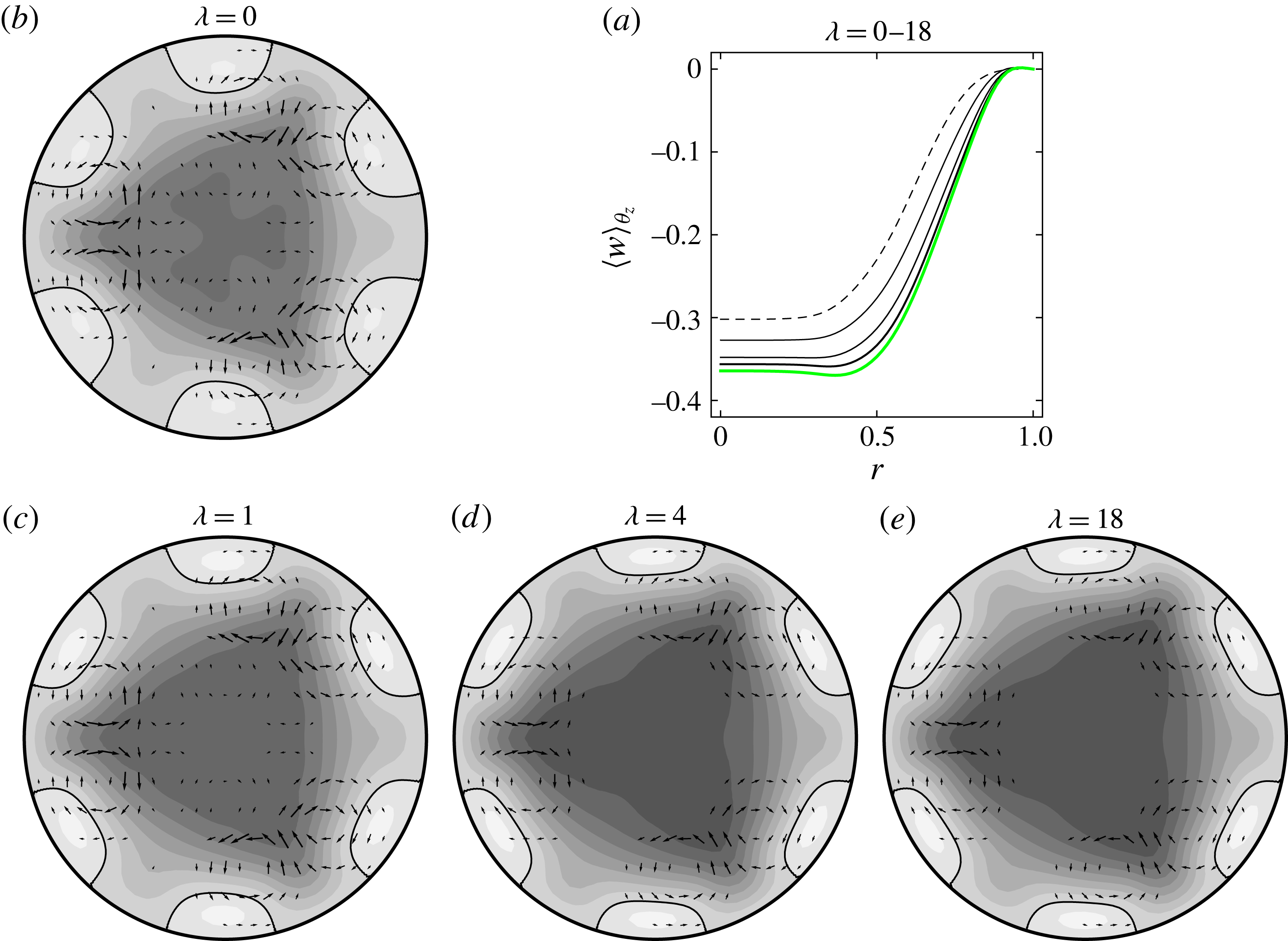
The velocity field of the waves converges to a limit as $\unicode[STIX]{x1D706}\rightarrow +\infty$ . This can be seen in the figures 10(a) and 11(a) for the radial profiles of axial velocity, with and without the base flow, averaged over $\unicode[STIX]{x1D703}$ and $z$ . Accordingly, the fields averaged over $z$ , in a pipe section, of the figures 10(b–e) and 11(b–e) converge to a precise pattern as $\unicode[STIX]{x1D706}\rightarrow +\infty$ . The asymptotic solution for $\unicode[STIX]{x1D706}\rightarrow +\infty$ may be viewed as the critical wave in a power-law fluid obeying to the rheological law (2.25), with $n_{C}=0.5$ . This solution, which corresponds approximately to the figure 11(e), displays even more clearly than the Newtonian solution of figure 11(b) three pairs of streamwise rolls and six attached fast streaks near the pipe wall. This observation and the continuity between all these waves proves that the self-sustaining process advocated in the introduction is at the origin of all these waves, even in the case of strongly shear-thinning fluids.

Figure 10.

For $n_{C}=0.5$ . (a) Total axial velocity $v_{z}$ averaged over $\unicode[STIX]{x1D703}$ and $z$ of the critical wave for different values of $\unicode[STIX]{x1D706}$ as in figure 2: the curves ordered by decreasing centreline velocities correspond to $\unicode[STIX]{x1D706}=0,1,2,4,18$ . (b–e) Axial average of the velocity field of the critical wave for various values of $\unicode[STIX]{x1D706}$ as indicated. The grey levels show the values of $\langle v_{z}\rangle _{z}$ with 9 regularly spaced contours $v_{z}=0.07$ (dark) to $0.63$ (light). The arrows show on a Cartesian grid the transverse velocity vectors $\boldsymbol{v}_{\bot }=\langle u\rangle _{z}\boldsymbol{e}_{r}+\langle v\rangle _{z}\boldsymbol{e}_{\unicode[STIX]{x1D703}}$ whose norm $\Vert \boldsymbol{v}_{\bot }\Vert \geqslant 0.003$ . The scale of the arrows is the same on all graphs: $\max \Vert \boldsymbol{v}_{\bot }\Vert$ decreases as $\unicode[STIX]{x1D706}$ increases.

Figure 11.

For $n_{C}=0.5$ . (a) Axial velocity $w=v_{z}-W_{b}$ averaged over $\unicode[STIX]{x1D703}$ and $z$ of the critical wave for different values of $\unicode[STIX]{x1D706}$ as in figure 10(a). (b–e) Axial average of the velocity field of the critical wave for various values of $\unicode[STIX]{x1D706}$ as indicated. The grey levels show the values of $\langle w\rangle _{z}$ with 9 regularly spaced contours $w=-0.35$ (dark) to $+0.05$ (light). The contour $w=0$ is shown with a black continuous line to evidence the fast streaks. The arrows show the transverse velocity vectors as in figure 10(b–e).

Figure 12.

For $n_{C}=0.5$ , for various values of $\unicode[STIX]{x1D706}$ as indicated. (a–c) Root-mean-square axial velocity $w^{\prime }(r,\unicode[STIX]{x1D703})$ ; continuous lines, 5 regularly spaced contours $w^{\prime }=0.025\overline{W}$ to $0.125\overline{W}$ ; dark grey (respectively light grey), low (respectively high) values. (d–f) $\langle \unicode[STIX]{x1D6E4}_{2}\rangle _{z}$ ; dashed line, first iso-contour $\unicode[STIX]{x1D6E4}_{2}=0.5$ ; continuous lines, 10 regularly spaced contours $\unicode[STIX]{x1D6E4}_{2}=1.5$ (near the centre) to $15$ (near the pipe wall).

Table 2.

For $n_{C}=0.5$ , various values of $\unicode[STIX]{x1D706}$ , value and radial position of the maximum root-mean-square axial velocity.

In order to better characterize the critical waves, in a manner that corresponds to the experiments advocated in the introduction, the root-mean-square value of the axial velocity is computed,

(5.9) $$\begin{eqnarray}\displaystyle w^{\prime }(r,\unicode[STIX]{x1D703})=v_{z}^{\prime }(r,\unicode[STIX]{x1D703})=\sqrt{\langle [v_{z}(r,\unicode[STIX]{x1D703},z-ct)-\langle v_{z}(r,\unicode[STIX]{x1D703},z-ct)\rangle _{t}]^{2}\rangle _{t}}. & & \displaystyle\end{eqnarray}$$

This field, normalized with the mean speed $\overline{W}$ , is characterized in the table 2 and shown in the figure 12(a–c). It is in the region of the rolls visible in figures 10 and 11 that $w^{\prime }$ is large. This strong dynamics of the rolls was already noticeable in the figure 1 of Faisst & Eckhardt (Reference Faisst and Eckhardt2003), and is also visible on the movie included as online supplementary material available at https://doi.org/10.1017/jfm.2017.149. A further characterization of this dynamics is given by the figure 13 $(a)$ , which displays profiles of $w(r,\unicode[STIX]{x1D703},z)$ at the place where $w^{\prime }$ is maximum for $n_{C}=0.5$ , $\unicode[STIX]{x1D706}=18$ , i.e. $r=0.59$ , $\unicode[STIX]{x1D703}=1.29$ . This figure confirms that the velocity field of the waves converges as $\unicode[STIX]{x1D706}\rightarrow +\infty$ .

Figure 13.

For $n_{C}=0.5$ , for the critical waves corresponding to the values of $\unicode[STIX]{x1D706}$ indicated in (b). (a) Axial velocity $w=v_{z}-W_{b}$ at $r=0.59$ , $\unicode[STIX]{x1D703}=1.29$ . (b) Ratio of the viscosity averaged over $\unicode[STIX]{x1D703}$ and $z$ to the wall viscosity.

Figure 14.

For $n_{C}=0.5$ and various values of $\unicode[STIX]{x1D706}$ as indicated. (a–d) Full line, invariant $\unicode[STIX]{x1D6E4}_{2}$ averaged over $\unicode[STIX]{x1D703}$ and $z$ of the critical wave; dashed line, invariant $\unicode[STIX]{x1D6E4}_{2}$ of the laminar flow, already displayed in figure 2(b). (e–g) Full line, viscosity $\unicode[STIX]{x1D702}$ averaged over $\unicode[STIX]{x1D703}$ and $z$ of the critical wave; dashed line, viscosity $\unicode[STIX]{x1D702}$ of the laminar flow, already displayed in figure 2(c). (h–k) Full line, product $\unicode[STIX]{x1D702}\unicode[STIX]{x1D6E4}_{2}$ averaged over $\unicode[STIX]{x1D703}$ and $z$ of the critical wave; dashed line, same product in the laminar flow.

Figure 15.

(a) For $n_{C}=0.5$ . $\star$ , onset wall-viscosity Reynolds number $\mathit{Re}_{w}(q_{cN};n_{C},\unicode[STIX]{x1D706})$ found by Roland et al. (Reference Roland, Plaut and Nouar2010); ●, after optimization of the wavenumber $q$ , critical wall-viscosity Reynolds number $\mathit{Re}_{wc}(n_{C},\unicode[STIX]{x1D706})$ ; ▾, critical mean-viscosity Reynolds number $\mathit{Re}_{mc}(n_{C},\unicode[STIX]{x1D706})$ ; grey (red online) curve, fit (5.15); upper dashed line, asymptotic value (5.16); lower dashed line, critical value of the Newtonian case $\mathit{Re}_{cN}$ (1.2). (b) ●, For $n_{C}=0.6$ , ▪, for $n_{C}=0.7$ , critical wall-viscosity Reynolds number $\mathit{Re}_{wc}(n_{C},\unicode[STIX]{x1D706})$ ; grey (red online) curves, fits (5.15), dashed lines, asymptotic values (5.19).

5.3.3 Rates of strain, viscosity and dissipation

A good understanding of all the properties of the waves, in the non-Newtonian case, requires a study of their viscosity field $\unicode[STIX]{x1D702}(r,\unicode[STIX]{x1D703},z)$ , which is itself a function of the field $\unicode[STIX]{x1D6E4}_{2}(r,\unicode[STIX]{x1D703},z)$ , the rate-of-strain intensity, defined in (2.5). This latter field multiplied by $\unicode[STIX]{x1D702}$ is the dissipated power per unit volume, which is physically meaningful for all fluids, Newtonian or not. In laminar or wave flows, the global kinetic energy balance is

(5.10) $$\begin{eqnarray}\displaystyle P_{diss}=\langle \unicode[STIX]{x1D702}\unicode[STIX]{x1D6E4}_{2}\rangle _{r\unicode[STIX]{x1D703}z}=\mathit{Re}_{0}\overline{W}G, & & \displaystyle\end{eqnarray}$$

i.e. the power dissipated by viscous effects is compensated by the power injected by pressure forces through the pressure gradient $G$ . Note that $P_{diss}$ is the averaged dissipated power by unit volume, rendered dimensionless by division by $\unicode[STIX]{x1D702}_{0}(W_{0}/a)^{2}$ with the notations of § 2.4. The relation (3.2) yields

(5.11) $$\begin{eqnarray}\displaystyle P_{diss}=\langle \unicode[STIX]{x1D702}\unicode[STIX]{x1D6E4}_{2}\rangle _{r\unicode[STIX]{x1D703}z}=\unicode[STIX]{x1D6FC}\overline{W}, & & \displaystyle\end{eqnarray}$$

where it is recalled that $\unicode[STIX]{x1D6FC}=4$ in Newtonian fluids, $\unicode[STIX]{x1D6FC}$ is smaller in non-Newtonian fluids (see § 4 and figure 4 a). The field $\unicode[STIX]{x1D6E4}_{2}$ axially averaged is shown in figure 12(d–f) for $n_{C}=0.5$ and three particular waves. Generally, $\unicode[STIX]{x1D6E4}_{2}$ vanishes, for symmetry reasons, at the pipe axis, and increases near the pipe wall, as already displayed in figure 2(b) for the laminar base flows. In wave flows, the highest rate of strain is localized near the fast streaks (compare figures 11 e and 12 f), where large velocity gradients are induced by the near-wall roll flows and the streak flows themselves. Obviously, the field $\unicode[STIX]{x1D6E4}_{2}$ in the critical waves converges to a well-defined limit as $\unicode[STIX]{x1D706}\rightarrow +\infty$ , as it was already shown for the laminar base flows in figure 2(b). This convergence is visible in the figure 14(a–d). Observe that, in the region near $r\simeq 0.6$ , where the roll flows are stronger, the average rate-of-strain intensity $\langle \unicode[STIX]{x1D6E4}_{2}\rangle _{\unicode[STIX]{x1D703}z}$ decreases, whatever $\unicode[STIX]{x1D706}$ . For $\unicode[STIX]{x1D706}=0$ , i.e. the Newtonian case, $\unicode[STIX]{x1D702}=1$ , the relation (5.11) gives

(5.12) $$\begin{eqnarray}\displaystyle P_{dissN}=\langle \unicode[STIX]{x1D6E4}_{2}\rangle _{r\unicode[STIX]{x1D703}z}=4\overline{W}. & & \displaystyle\end{eqnarray}$$

In the case of the laminar, Hagen–Poiseuille flow,

(5.13) $$\begin{eqnarray}\displaystyle P_{dissN}=\langle \unicode[STIX]{x1D6E4}_{2}\rangle _{r\unicode[STIX]{x1D703}z}=2\int _{0}^{1}\langle \unicode[STIX]{x1D6E4}_{2}\rangle _{\unicode[STIX]{x1D703}z}r\,\text{d}r=2, & & \displaystyle\end{eqnarray}$$

which is coherent with the dashed profile of figure 14(a). On the other hand, in the critical EFKW wave,

(5.14) $$\begin{eqnarray}\displaystyle P_{dissN}=\langle \unicode[STIX]{x1D6E4}_{2}\rangle _{r\unicode[STIX]{x1D703}z}=2\int _{0}^{1}\langle \unicode[STIX]{x1D6E4}_{2}\rangle _{\unicode[STIX]{x1D703}z}r\,\text{d}r=4\overline{W}_{cN}=1.54, & & \displaystyle\end{eqnarray}$$

which is coherent with the continuous profile of figure 14(a). The tendencies observed in figure 14(a), i.e. lower (respectively higher) rate of strain near $r\simeq 0.6$ (respectively $r\simeq 1$ ) in the wave than in the laminar flow, persist in the non-Newtonian case: the profiles of the figure 14(a–d) are all similar, the main effect being an increase in magnitude, already encountered in figure 2(b). Because the non-Newtonian fluids studied are shear thinning, smaller values of $\unicode[STIX]{x1D6E4}_{2}$ imply larger values of $\unicode[STIX]{x1D702}$ (2.19): indeed the profiles of the figure 14(e–g) show a bump of $\unicode[STIX]{x1D702}$ near $r\simeq 0.6$ . Since the relation (2.19) is nonlinear, $\langle \unicode[STIX]{x1D702}\rangle _{\unicode[STIX]{x1D703}z}$ is not the viscosity evaluated at $\langle \unicode[STIX]{x1D6E4}_{2}\rangle _{\unicode[STIX]{x1D703}z}$ , i.e. the link between the profiles of the figure 14(b–d) and those of the figure 14(e–g) is not straightforward. This is in particular visible near the pipe wall, where $\langle \unicode[STIX]{x1D6E4}_{2}\rangle _{\unicode[STIX]{x1D703}z}$ in the wave is larger than $\unicode[STIX]{x1D6E4}_{2}$ in the laminar flow, though $\langle \unicode[STIX]{x1D702}\rangle _{\unicode[STIX]{x1D703}z}$ in the wave is $\unicode[STIX]{x1D702}_{w}$ . In line with the relation (5.11), and the fact that $\overline{W}$ in wave flows is smaller than $\overline{W}_{b}$ in the laminar flows, the figure 14(h–j) shows that the product $\unicode[STIX]{x1D702}\unicode[STIX]{x1D6E4}_{2}$ , the local dissipation rate, decreases in average in wave flows.

A master curve for the averaged viscosity profiles can be obtained by measuring the viscosity in units of the wall viscosity $\unicode[STIX]{x1D702}_{w}$ , as it has already been done for the laminar flows in figure 2(d). The figure 13(b) shows that, as $\unicode[STIX]{x1D706}\rightarrow +\infty$ , $\langle \unicode[STIX]{x1D702}\rangle _{\unicode[STIX]{x1D703}z}/\unicode[STIX]{x1D702}_{w}$ converges to a curve which corresponds quite probably to the one of the power-law fluid critical wave, the viscosity of which diverges as $r\rightarrow 0^{+}$ .

If one comes back to the figure 14(e–g), it is clear that the bulk average mean viscosity $\overline{\unicode[STIX]{x1D702}}_{c}$ of the critical waves is slightly larger than the bulk average mean viscosity $\overline{\unicode[STIX]{x1D702}}_{b}$ of the laminar flows, which has been studied in § 3.3. This is confirmed by the triangles in the figure 3(b). Note that, for $\unicode[STIX]{x1D706}\geqslant 4$ , $\overline{\unicode[STIX]{x1D702}}_{c}(n_{C},\unicode[STIX]{x1D706})\simeq \overline{\unicode[STIX]{x1D702}}_{bpl}(n_{C},\unicode[STIX]{x1D706})$ within $\pm 18\,\%$ .

5.3.4 Critical Reynolds numbers

The figure 8 suggests that the critical wall-viscosity Reynolds number $\mathit{Re}_{wc}(n_{C},\unicode[STIX]{x1D706})$ , which corresponds to the minima of the curves in this figure, converges to a finite limit as $\unicode[STIX]{x1D706}\rightarrow +\infty$ . Indeed, a fit of the form

(5.15) $$\begin{eqnarray}\displaystyle \mathit{Re}_{wc}(n_{C},\unicode[STIX]{x1D706})=\mathit{Re}_{wcpl}(n_{C})+\unicode[STIX]{x1D6FE}(n_{C})\,\unicode[STIX]{x1D706}^{-3/2}, & & \displaystyle\end{eqnarray}$$

evaluated on the last 3 data disk points of figure 15(a), for $\unicode[STIX]{x1D706}\geqslant 10$ , yields a curve that describes well the 8 data disk points of figure 15(a) with $\unicode[STIX]{x1D706}\geqslant 3$ . From this fit one extracts the critical value for a power-law fluid

(5.16) $$\begin{eqnarray}\displaystyle \mathit{Re}_{wcpl}(n_{C}=0.5)=2890. & & \displaystyle\end{eqnarray}$$

The optimization of the wavenumber $q$ has a dramatic effect; if it is not performed, as it was the case in Roland et al. (Reference Roland, Plaut and Nouar2010), one obtains the upper curve with the stars in figure 15(a), with much higher values of $\mathit{Re}_{w}$ . One can question the choice of the characteristic viscosity used to define the critical Reynolds number. A remarkable result of figure 15(a) is that, if one uses a Reynolds number constructed on the bulk average mean viscosity $\overline{\unicode[STIX]{x1D702}}_{c}$ of the critical waves,

(5.17) $$\begin{eqnarray}\displaystyle \mathit{Re}_{mc}(n_{C},\unicode[STIX]{x1D706})=\mathit{Re}_{wc}(n_{C},\unicode[STIX]{x1D706})\,\unicode[STIX]{x1D702}_{w}(n_{C},\unicode[STIX]{x1D706})/\overline{\unicode[STIX]{x1D702}}_{c}(n_{C},\unicode[STIX]{x1D706}), & & \displaystyle\end{eqnarray}$$

with the exact values displayed by the triangles in the figure 3(b), one obtains the curve with the triangles in the figure 15(a), which is almost flat. Thus, approximately, $\mathit{Re}_{mc}(n_{C},\unicode[STIX]{x1D706})\simeq \mathit{Re}_{cN}=1251$ . Using this approximation, and $\overline{\unicode[STIX]{x1D702}}_{c}(n_{C},\unicode[STIX]{x1D706})\simeq \overline{\unicode[STIX]{x1D702}}_{bpl}(n_{C},\unicode[STIX]{x1D706})$ , in (5.17), we can propose, with the help of (3.12), the analytic formula

(5.18) $$\begin{eqnarray}\displaystyle \mathit{Re}_{wcpl}(n_{C})\simeq 1251\,\overline{\unicode[STIX]{x1D702}}_{bpl}(n_{C},\unicode[STIX]{x1D706})/\unicode[STIX]{x1D702}_{wpl}(n_{C},\unicode[STIX]{x1D706})=834\,n_{C}/(n_{C}-1/3). & & \displaystyle\end{eqnarray}$$

5.4 Validation - asymptotic power-law regime for $n_{C}\geqslant 0.5$

In order to validate the analytic formula (5.18), computations have been performed with $n_{C}=0.6$ and $0.7$ , by continuation starting from the solutions obtained with $n_{C}=0.5$ . The critical values of the wavenumber $q$ increase, i.e. they are closer to the Newtonian value (1.9): for instance $q_{c}(0.6,18)=2.07$ , $q_{c}(0.7,18)=2.16$ (compare with figure 9 $a$ ). The critical wall-viscosity Reynolds numbers obtained are displayed in figure 15 $(b)$ . With fits of the form (5.15), we determine the asymptotic values

(5.19a,b ) $$\begin{eqnarray}\displaystyle \mathit{Re}_{wcpl}(n_{C}=0.6)=2175,\quad \mathit{Re}_{wcpl}(n_{C}=0.7)=1782. & & \displaystyle\end{eqnarray}$$

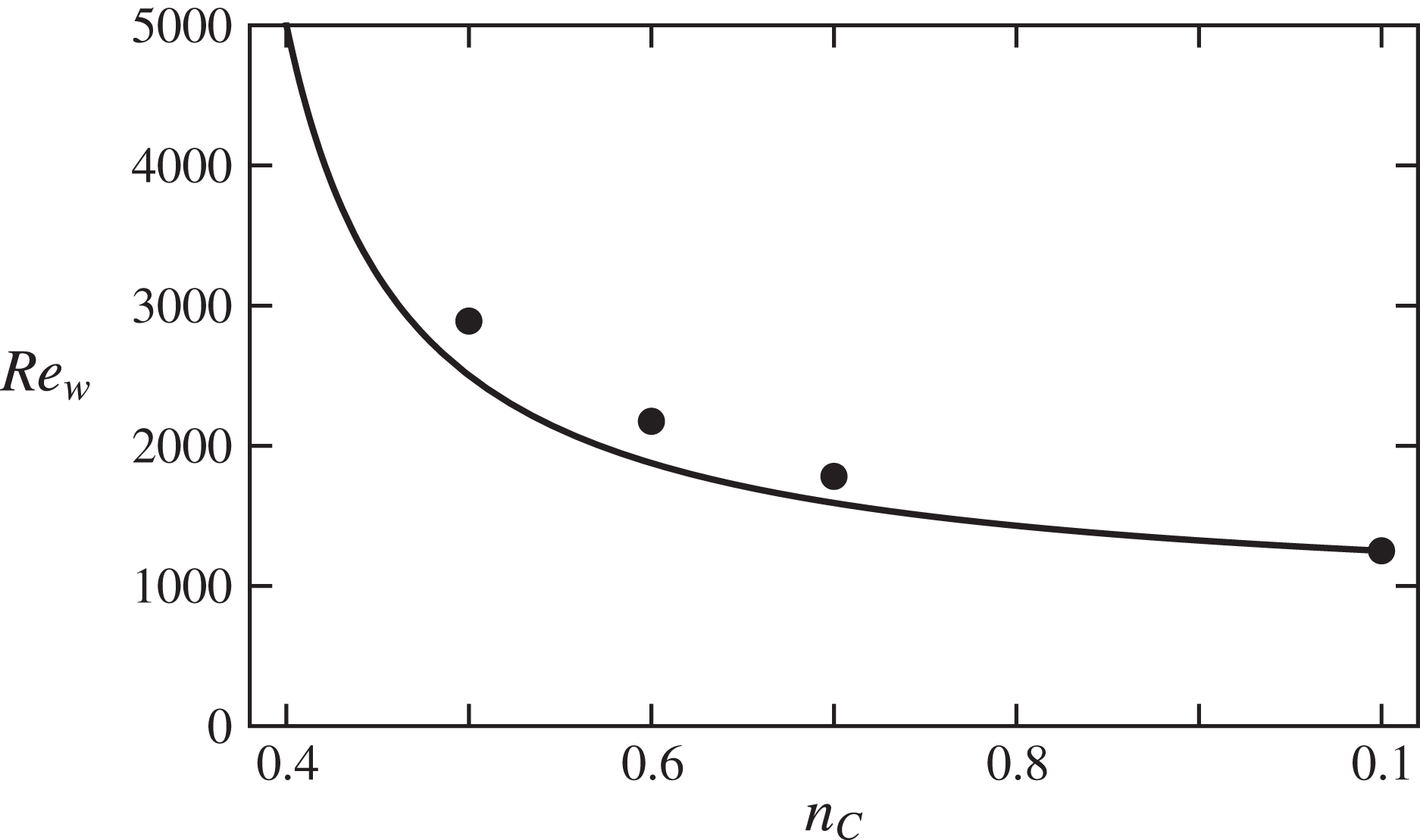
As shown in the figure 16, the formula (5.18) yields a reasonable estimate of $\mathit{Re}_{wcpl}(n_{C})$ in both cases.

Figure 16.

●, Asymptotic values of the critical wall-viscosity Reynolds number $\mathit{Re}_{wcpl}(n_{C})$ for $n_{C}=0.5,0.6,0.7$ together with the Newtonian value $\mathit{Re}_{wcpl}(1)=\mathit{Re}_{cN}$ ; continuous curve, formula (5.18).

6.1 Newtonian fluid

Consider the critical EFKW wave that develops, in a Newtonian pipe flow, on top of the laminar Hagen–Poiseuille flow with centreline velocity $W_{0}$ and pressure gradient $G_{0}$ . The dimensional mass flux of this laminar flow is $W_{0}\overline{W}_{bN}$ with $\overline{W}_{bN}=0.5$ , whereas the dimensional mass flux of the wave is smaller, $W_{0}\overline{W}_{cN}$ with $\overline{W}_{cN}=0.384$ (§ 5.3.1). The laminar flow at the same mass flux corresponds to a centreline velocity $W_{1}$ such that

(6.1) $$\begin{eqnarray}\displaystyle W_{1}\overline{W}_{bN}=W_{0}\overline{W}_{cN}\quad \text{i.e.}~W_{1}=W_{0}\overline{W}_{cN}/\overline{W}_{bN}=0.768W_{0}. & & \displaystyle\end{eqnarray}$$

The pressure gradient in this laminar flow is proportional to the centreline velocity, $G_{1}=0.768G_{0}$ . Hence the pressure gradient increase factor at constant mass flux is

(6.2) $$\begin{eqnarray}\displaystyle A=G_{0}/G_{1}=W_{0}/W_{1}=\overline{W}_{bN}/\overline{W}_{cN}=1.30. & & \displaystyle\end{eqnarray}$$

6.2 Non-Newtonian Carreau fluid

Consider a critical wave computed in a given pipe, for a given non-Newtonian fluid, given pressure gradient $G_{0}$ characterized by the corresponding centreline laminar base flow velocity $W_{0}$ , hence given parameters $\mathit{Re}_{0}$ and $\unicode[STIX]{x1D706}=\unicode[STIX]{x1D706}_{C}W_{0}/a$ . The dimensional mass flux of this laminar flow is $W_{0}\overline{W}_{b}(n_{C},\unicode[STIX]{x1D706})$ , whereas the dimensional mass flux of the wave is smaller, $W_{0}\overline{W}_{c}(n_{C},\unicode[STIX]{x1D706})$ (§ 5.3.1). The laminar base flow of the same fluid in the same pipe with the same mass flux corresponds to a smaller value of the centreline velocity $W_{1}$ , smaller value of $\unicode[STIX]{x1D706}$ , $\unicode[STIX]{x1D706}_{1}=\unicode[STIX]{x1D706}_{C}W_{1}/a$ , such that

(6.3) $$\begin{eqnarray}\displaystyle W_{1}\overline{W}_{b}(n_{C},\unicode[STIX]{x1D706}_{1})=W_{0}\overline{W}_{c}(n_{C},\unicode[STIX]{x1D706})\quad \text{i.e.}~\unicode[STIX]{x1D706}_{1}\overline{W}_{b}(n_{C},\unicode[STIX]{x1D706}_{1})=\unicode[STIX]{x1D706}\overline{W}_{c}(n_{C},\unicode[STIX]{x1D706}) & & \displaystyle\end{eqnarray}$$

after multiplication by $\unicode[STIX]{x1D706}_{C}/a$ . The function $\unicode[STIX]{x1D706}_{1}\mapsto \overline{W}_{b}(n_{C},\unicode[STIX]{x1D706}_{1})$ increases (figure 3 a), hence $\unicode[STIX]{x1D706}_{1}\mapsto \unicode[STIX]{x1D706}_{1}\overline{W}_{b}(n_{C},\unicode[STIX]{x1D706}_{1})$ increases, equation (6.3) defines $\unicode[STIX]{x1D706}_{1}$ without ambiguity. For large $\unicode[STIX]{x1D706}$ , $\overline{W}_{\!c}(n_{C},\unicode[STIX]{x1D706})\simeq \overline{W}_{\!cpl}(n_{C})$ , $\unicode[STIX]{x1D706}_{1}$ is large and $\overline{W}_{\!b}(n_{C},\unicode[STIX]{x1D706}_{1})\simeq \overline{W}_{\!bpl}(n_{C})$ . Hence the solution of (6.3) approaches

(6.4) $$\begin{eqnarray}\displaystyle \unicode[STIX]{x1D706}_{1pl}=\unicode[STIX]{x1D706}\overline{W}_{cpl}(n_{C})/\overline{W}_{bpl}(n_{C})=0.69\unicode[STIX]{x1D706} & & \displaystyle\end{eqnarray}$$

for $n_{C}=0.5$ , according to (5.8). Because of (3.2), the dimensional pressure gradient in the reference laminar flow i.e. in the wave flow is

(6.5) $$\begin{eqnarray}\displaystyle G_{0}=G\,\unicode[STIX]{x1D70C}W_{0}^{2}/a=\unicode[STIX]{x1D6FC}(n_{C},\unicode[STIX]{x1D706})\mathit{Re}_{0}^{-1}\,\unicode[STIX]{x1D70C}W_{0}^{2}/a=\unicode[STIX]{x1D6FC}(n_{C},\unicode[STIX]{x1D706})\,\unicode[STIX]{x1D70C}W_{0}\unicode[STIX]{x1D708}_{0}/a^{2}. & & \displaystyle\end{eqnarray}$$

Accordingly the dimensional pressure gradient in the laminar flow with the same mass flux is

(6.6) $$\begin{eqnarray}\displaystyle G_{1}=\unicode[STIX]{x1D6FC}(n_{C},\unicode[STIX]{x1D706}_{1})\,\unicode[STIX]{x1D70C}W_{1}\unicode[STIX]{x1D708}_{0}/a^{2}. & & \displaystyle\end{eqnarray}$$

Hence the pressure gradient increase factor at constant mass flux is

(6.7) $$\begin{eqnarray}\displaystyle A(n_{C},\unicode[STIX]{x1D706})=G_{0}/G_{1}=\unicode[STIX]{x1D706}\unicode[STIX]{x1D6FC}(n_{C},\unicode[STIX]{x1D706})/(\unicode[STIX]{x1D706}_{1}\unicode[STIX]{x1D6FC}(n_{C},\unicode[STIX]{x1D706}_{1})). & & \displaystyle\end{eqnarray}$$

At large $\unicode[STIX]{x1D706}$ , i.e. large $\unicode[STIX]{x1D706}_{1}\simeq \unicode[STIX]{x1D706}_{1pl}$ given by (6.4), the power-law formula (4.6) yields the approximation

(6.8) $$\begin{eqnarray}\displaystyle A(n_{C},\unicode[STIX]{x1D706})\simeq A_{pl}(n_{C})=(\unicode[STIX]{x1D706}/\unicode[STIX]{x1D706}_{1pl})^{n_{C}}=(\overline{W}_{bpl}(n_{C})/\overline{W}_{cpl}(n_{C}))^{n_{C}}. & & \displaystyle\end{eqnarray}$$

The Newtonian formula (6.2) is recovered in the limit $n_{C}\rightarrow 1$ . For instance,

(6.9) $$\begin{eqnarray}\displaystyle A_{pl}(n_{C}=0.5)=1.20. & & \displaystyle\end{eqnarray}$$

Physically, the nonlinear relation between the pressure gradient and the centreline velocity in laminar flows (6.5), in the power-law limit,

(6.10) $$\begin{eqnarray}\displaystyle G_{0pl}=\unicode[STIX]{x1D6FC}_{pl}(n_{C},\unicode[STIX]{x1D706})\,\unicode[STIX]{x1D70C}W_{0}\unicode[STIX]{x1D708}_{0}/a^{2}=2a^{-n_{C}-1}\unicode[STIX]{x1D70C}\unicode[STIX]{x1D708}_{0}\unicode[STIX]{x1D706}_{C}^{n_{C}-1}(1+1/n_{C})^{n_{C}}\,W_{0}^{n_{C}}, & & \displaystyle\end{eqnarray}$$

leads to the fact that the pressure gradient increase factor $A_{pl}$ is the mass flux reduction factor (5.8) at the power $-n_{C}$ . Thus the pressure gradient increase factor in the power-law fluids (6.8) or (6.9) is smaller than in the Newtonian fluid (6.2); this is remarkable.

Note finally that the computation of $\unicode[STIX]{x1D706}_{1}$ from the full equation (6.3) and then of $A$ from (6.7) shows a fast convergence, as $\unicode[STIX]{x1D706}$ increases, to the power-law limit; for instance $A(n_{C}=0.5,\unicode[STIX]{x1D706}=1)=1.22$ is already $A_{pl}(n_{C}=0.5)$ within 2 %.