




1. Introduction
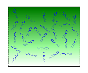
The collective motion in an active suspension of chemotactic swimmers has been explored through experiments in a variety of settings (Budrene & Berg Reference Budrene and Berg1991, Reference Budrene and Berg1995; Dombrowski et al. Reference Dombrowski, Cisneros, Chatkaew, Goldstein and Kessler2004; Sokolov et al. Reference Sokolov, Aranson, Kessler and Goldstein2007, Reference Sokolov, Goldstein, Feldchtein and Aranson2009). In particular, the role of chemotaxis in symmetry breaking and the triggering of an instability (Hillesdon & Pedley Reference Hillesdon and Pedley1996; Saintillan & Shelley Reference Saintillan and Shelley2008b; Kasyap & Koch Reference Kasyap and Koch2012, Reference Kasyap and Koch2014; Lushi Reference Lushi2016) has received wide attention due to its relevance in a variety of natural systems. The current work explores the creation of active stress-driven instabilities in a confined suspension of autochemotactic swimmers.
The modelling of self-propelled swimmers as force dipoles (Spagnolie & Lauga Reference Spagnolie and Lauga2012) is adopted when the suspensions are dilute, with the flow field being accurately represented by considering solely the far-field hydrodynamics of the individual swimmers. A single Escherichia coli bacterium generates an extensile flow field as a result of its self-propulsion and is classified as a pusher-type swimmer. Conversely, the algae Chlamydomonas reinhardtii creates a contractile flow field as it swims through the beating of its twin flagella, and is classified as a puller. Pushers and pullers differ in the sign of the dipole moment, with its actual magnitude being dependent on the cell structure of the particular species under consideration. In addition, motile swimmers rarely traverse along straight lines for long times and undergo sudden random changes in orientation, a phenomenon known as tumbling, that allows them to sample their surrounding environment in search of nutrients. The motion of the swimmers through a medium can thus be thought of as a random walk with a diffusivity that arises from the tumbling and is purely athermal in nature. The hydrodynamic flow field generated by swimming and the phenomenon of tumbling are two important aspects to account for in the modelling of swimmer dynamics at the microscopic scale.
In addition to performing a random walk, swimmers such as E. coli tend to migrate to regions of favourable chemical concentration, a feature known as chemotaxis that contributes to the survival of the organism (Berg Reference Berg2008). The mechanism involved in setting up the preferential migration of swimmers depends greatly on the species under consideration. For example, swimmers such as E. coli and Bacillus subtilis alter their tumbling frequency to tumble less frequently when they are aligned favourably to an attractant gradient, and vice versa when they are aligned away from the attractant gradient (Rivero et al. Reference Rivero, Tranquillo, Buettner and Lauffenburger1989; Chen, Ford & Cummings Reference Chen, Ford and Cummings2003). The chemotactic response of the swimmers in a suspension thus plays a crucial role in determining the orientation distribution of the swimmers, as in the absence of any such chemical gradients the swimmers execute a random walk. In general, the stimulus dictating the preferential swimming is not limited to gradients in a chemical concentration field. Many Chlamydomonas species of algae exhibit phototaxis (Jékely Reference Jékely2009; Martin et al. Reference Martin, Barzyk, Bertin, Peyla and Rafai2016; Brun-Cosme-Bruny et al. Reference Brun-Cosme-Bruny, Förtsch, Zimmermann, Bertin, Peyla and Rafaï2020), wherein the swimmers tend to migrate towards regions of higher intensity of light. Magnetotaxis refers to the preferential swimming of organisms along the local magnetic field as sampled by a swimmer (Blakemore Reference Blakemore1975), and it has been seen in species of Magnetococcus. While the effects of chemotaxis and phototaxis are triggered through the sampling of the stimuli by the swimmer along its trajectory, the magnetotactic response to the instantaneous magnetic field results in a far greater migration speed.
In E. coli, the secretion of an attractant has been observed when individual swimmers are subjected to cellular stresses that necessitate the formation of multicellular structures for survival (Mittal et al. Reference Mittal, Budrene, Brenner and Van Oudenaarden2003), in which the phenomenon of autochemotaxis and self-signalling play a critical role. Experiments by Budrene & Berg (Reference Budrene and Berg1991, Reference Budrene and Berg1995) involving suspensions of autochemotactic swimmers have revealed the formation of swimmer clusters at specific locations in the domain. An early work that aims to explore the instabilities arising in such systems was given by Keller & Segel (Reference Keller and Segel1970), wherein the authors have attempted to model travelling bands of E. coli by considering a pair of diffusion equations governing the swimmer density and substrate concentration fields, with appropriate additional terms accounting for the chemotactic flux and the substrate consumption by the swimmer. Brenner, Levitov & Budrene (Reference Brenner, Levitov and Budrene1998) considered the system of chemotactic swimmers, wherein the individual swimmers generate an attractant that enables cluster formation through self-signalling. They showed that the solution for the autochemotactic system exhibits a finite-time blowup and used it to describe the patterns observed by Budrene & Berg (Reference Budrene and Berg1991, Reference Budrene and Berg1995).
In the literature, the instabilities observed in active suspensions of pullers have emerged from the preferential swimmer motility. For instance, the observed instabilities contributing to the formation of bioconvective patterns (Kessler Reference Kessler1984) were mostly enabled by gyrotaxis. Gyrotaxis refers to the preference of algae such as Chlamydomonas nivalis to swim vertically upwards, due to a balance between the viscous and gravitational torques that arise due to the cells being bottom-heavy. Since the swimmers are denser than the aqueous medium they are present in, an instability similar to Rayleigh–Bénard convection has been observed experimentally (Kessler Reference Kessler1985a,Reference Kesslerb) and theoretically (Kessler Reference Kessler1986; Pedley, Hill & Kessler Reference Pedley, Hill and Kessler1988; Hill, Pedley & Kessler Reference Hill, Pedley and Kessler1989; Pedley & Kessler Reference Pedley and Kessler1990) in these systems. In addition, this form of taxis is of ecological importance in the layer formation in certain plankton species (Sullivan, Donaghay & Rines Reference Sullivan, Donaghay and Rines2010) and the formation of algal blooms (Nielsen, Kiørboe & Bjørnsen Reference Nielsen, Kiørboe and Bjørnsen1990) in coastal areas. Aside from chemotaxis, the hydrodynamics associated with the self-propulsion of the swimmers also plays a critical role in the growth of instabilities in active suspensions (Dombrowski et al. Reference Dombrowski, Cisneros, Chatkaew, Goldstein and Kessler2004; Sokolov et al. Reference Sokolov, Aranson, Kessler and Goldstein2007, Reference Sokolov, Goldstein, Feldchtein and Aranson2009). In this regard, the instabilities in suspensions of pushers (Saintillan & Shelley Reference Saintillan and Shelley2008a; Kasyap & Koch Reference Kasyap and Koch2012, Reference Kasyap and Koch2014) have largely been attributed to the creation of an active stress-driven flow in the domain. The active stress arising from the propulsion of these swimmers is dependent upon the instantaneous microstructure of the suspension. The swimmers are suspended in the fluid medium and the term ‘microstructure’ refers to the position and orientation of each individual swimmer (the suspended phase) at a given time. By employing a kinetic-theory-based formulation, the subsequent works by Saintillan & Shelley (Reference Saintillan and Shelley2008a,Reference Saintillan and Shelleyb) and Subramanian & Koch (Reference Subramanian and Koch2009) introduce a probability distribution function associated with the microstructure of the suspension. Thus  $\varOmega (\boldsymbol {x},\boldsymbol {p},t)$ is a probability distribution function associated with finding a swimmer at a location
 $\boldsymbol {x}$ having an orientation
 $\boldsymbol {p}$ and is governed by the kinetic equation as described in Subramanian & Koch (Reference Subramanian and Koch2009) as follows:
 \begin{equation} \frac{\partial \varOmega}{\partial t} + {\boldsymbol{\nabla}} \boldsymbol{\cdot} \left[( U_s \boldsymbol{p} +\boldsymbol{u} ) \varOmega \right] + {\boldsymbol{\nabla}} \boldsymbol{\cdot} \left( \boldsymbol{\dot{p}} \varOmega \right) + \left( \frac{\varOmega}{\tau} - \frac{1}{4 {\rm \pi}} \int \frac{\varOmega}{\tau} \, {\rm d}\boldsymbol{p} \right) = 0. \end{equation}
Here,  $U_s$ and
 $L$ are the swimming speed and length of the organism, while
 $\tau ^{-1}$ represents the tumbling frequency associated with the individual swimmer motility. The first three terms represent the material derivative of
 $\varOmega$ in the six-dimensional phase space spanned by the position and orientation of a swimmer. The last two terms act as a source and sink with respect to the distribution function due to the tumbling behaviour of the swimmers. The form of
 $\varOmega$ is essential in estimating the active stress in the suspension and usually requires solving the full kinetic equation (1.1).
Subramanian, Koch & Fitzgibbon (Reference Subramanian, Koch and Fitzgibbon2011) were able to derive a form of the active stress relevant to the continuum formulation adopted in this paper by arguing that the time scale over which the material derivative becomes prominent is much larger than the time scale associated with the tumbling events. Thus at leading order, for perfectly isotropic tumbles, the distribution function  $\varOmega (\boldsymbol {x},\boldsymbol {p},t)$ is given by a balance between the source and sink terms in the kinetic equation (1.1) that arises from the phenomenon of tumbling,
 \begin{equation} \left(\frac{\varOmega}{\tau} - \frac{1}{4 {\rm \pi}} \int \frac{\varOmega}{\tau} {\rm d}\boldsymbol{p}\right) = 0. \end{equation}
The biased migration of the swimmers, due to some form of taxis, has a direct effect on the microstructure of the suspension. The preferential swimming is introduced into the modelling by accounting for the variation in the tumbling frequency  $\tau$ as a function of the swimmer orientation
 $\boldsymbol {p}$. Rivero et al. (Reference Rivero, Tranquillo, Buettner and Lauffenburger1989) and Chen et al. (Reference Chen, Ford and Cummings2003) have established through experiments that
 $\tau ^{-1}$ in chemotactic suspensions has a biphasic functional form as follows:
 \begin{equation} \tau^{{-}1} =\begin{cases} \tau_0^{{-}1} \exp({-\xi \boldsymbol{p} \boldsymbol{\cdot} \boldsymbol{g}}) & \text{if}\ \boldsymbol{p} \boldsymbol{\cdot} \boldsymbol{g} > 0,\\ \tau_0^{{-}1} & \text{if}\ \boldsymbol{p} \boldsymbol{\cdot} \boldsymbol{g} < 0. \end{cases} \end{equation}
Here,  $\xi = \chi U_s | \boldsymbol {\nabla } c |$ gives the strength of chemotaxis, where
 $\chi$ is the sensitivity of the bacterium to the presence of an attractant gradient, and
 $|\boldsymbol {\nabla } c|$ indicates the magnitude of the attractant gradient. In the current work, we adopt the model for the stopping rate of swimming as given in Bearon & Pedley (Reference Bearon and Pedley2000), by considering
 $\boldsymbol {g} = \boldsymbol {\nabla }c / | \boldsymbol {\nabla }c |$ to be along the local spatial gradient of the concentration field. Using the linearized form of the tumbling frequency shown in (1.3), which is justified for weakly chemotactic suspensions
 $(\xi \ll 1)$, Subramanian et al. (Reference Subramanian, Koch and Fitzgibbon2011) and Kasyap & Koch (Reference Kasyap and Koch2012) have solved (1.2) to obtain an analytical expression for the probability distribution function
 $\varOmega (\boldsymbol {x},\boldsymbol {p},t)$ as follows:
 \begin{equation} \varOmega(\boldsymbol{x},\boldsymbol{p},t) = \begin{cases} \dfrac{n}{4 {\rm \pi}} \left[ 1+ \left(\boldsymbol{p} \boldsymbol{\cdot} \boldsymbol{g} - \dfrac{1}{4} \right) \xi \right] & \text{if}\ \boldsymbol{p} \boldsymbol{\cdot} \boldsymbol{g} > 0,\\ \dfrac{n}{4 {\rm \pi}} \left[ 1 - \dfrac{1}{4} \xi \right] & \text{if} \ \boldsymbol{p} \boldsymbol{\cdot} \boldsymbol{g} < 0. \end{cases} \end{equation}
The use of the linearized form of the tumbling frequency given in (1.3) citing weak chemotaxis  $(\xi \ll 1)$ is justified when the channel width is sufficiently large (see Bearon & Pedley (Reference Bearon and Pedley2000) for the estimate of the chemotactic strength
 $\xi$). For the case of the channel width being
 $500\,\mathrm {\mu }{\rm m}$,
 $\xi \approx 0.1$, which makes the linearization appropriate.
The role of hydrodynamics in enabling pattern formation in confined suspensions of active fluids was demonstrated by Kasyap & Koch (Reference Kasyap and Koch2012, Reference Kasyap and Koch2014) through a continuum formulation, wherein they showed that the biased migration of swimmers along an imposed chemical gradient is capable of creating a flow instability that results in an aggregation of swimmers. In both papers, the attractant field was fixed externally to vary linearly across the domain height. Aside from these continuum formulations, Saintillan & Shelley (Reference Saintillan and Shelley2008a,Reference Saintillan and Shelleyb, Reference Saintillan and Shelley2013) make use of kinetic-theory-based simulations to explore the pattern formation and clustering in active suspensions of fluids, wherein an equation similar to (1.1) is solved in its entirety. More recently, Ezhilan, Pahlavan & Saintillan (Reference Ezhilan, Pahlavan and Saintillan2012), Lushi, Goldstein & Shelley (Reference Lushi, Goldstein and Shelley2012) and Lushi (Reference Lushi2016) have used kinetic simulations to explore the hydrodynamic stability of an autochemotactic suspension of pushers and pullers about a homogeneous base state.
In this paper, we are interested in the role of self-signalling between swimmers through the secretion of an attractant, on the suppression and amplification of the active stress-driven instabilities observed in these systems, through a continuum formulation. In § 2 the problem is formulated as a suspension of swimmers contained in a channel – the top and bottom wall of which are maintained at a constant concentration of the attractant – a set-up that was motivated by the hydrogel-based microfluidic device proposed by Cheng et al. (Reference Cheng, Heilman, Wasserman, Archer, Shuler and Wu2007). Section 3 begins with the formulation of linear stability calculation of the system, wherein the attractant transport is governed by a pseudosteady state equation that is devoid of the convective transport of the attractant. Subsequently, the base state profiles are derived for different attractant secretion rates ( $Da$). In § 3.1, the stability equations are solved numerically and analytically in the long-wave regime (
 $k \ll 1$) and the regions of stability are characterized. Section 3.2 addresses the finite wavenumber stability calculation for the system. Finally, in § 4 we address the role of convective transport of the attractant field due to the flow set up by the active stresses in the system, on the stability calculation of § 3.
2. Problem formulation
The flow resulting from the active stresses present in the suspension is incompressible and is governed by the Stokes equation, with the inertial terms being absent due to the low Reynolds number of the problem,
 \begin{gather} {\boldsymbol{\nabla}} \boldsymbol{\cdot} {\boldsymbol{u}} = 0, \end{gather}
 \begin{gather}- {\boldsymbol{\nabla}} p + \mu {{\nabla}}^{2} {\boldsymbol{u}} + {\boldsymbol{\nabla}} \boldsymbol{\cdot} {\boldsymbol{T}}^{\boldsymbol{B}} = 0. \end{gather}
Here,  ${\boldsymbol {T}}^{\boldsymbol {B}}$ represents the stress on the fluid arising due the motility of the swimmers within the suspension and can be written as an orientational average of the stress contribution from each individual swimmer (Subramanian & Koch Reference Subramanian and Koch2009),
 \begin{equation} {\boldsymbol{T}}^{\boldsymbol{B}}(\boldsymbol{x},t) ={-}C \mu U_s L^{2} \int \varOmega({\boldsymbol{x}},{\boldsymbol{p}},t) \left({\boldsymbol{p}}{\boldsymbol{p}} - \frac{{\boldsymbol{I}}}{3} \right) {\rm d}{\boldsymbol{p}}, \end{equation}
where  $C$ is the dipole moment associated with the hydrodynamic field generated by the swimmers motility. Using the form of
 $\varOmega$ given in (1.4) as derived in Kasyap & Koch (Reference Kasyap and Koch2012), the active stress
 ${\boldsymbol {T}}^{\boldsymbol {B}}$ turns out to be
 \begin{equation} {\boldsymbol{T}}^{\boldsymbol{B}} = n \boldsymbol{S}, \end{equation}
where
 \begin{equation} \boldsymbol{S} ={-}\frac{C}{16}\mu U_{s} L^{2} \xi\left({\boldsymbol{g}} {\boldsymbol{g}} - \frac{1}{3}\boldsymbol{I}\right). \end{equation}
Here,  $n$ is the swimmer density field and
 $\boldsymbol {S}$ is the single particle stresslet. While the second moment of the distribution function
 $\varOmega$ describes the active stress in the system, a zeroth moment of (1.1) results in an advection–diffusion equation that governs the evolution of the swimmer number density as seen in (2.6) (Kasyap & Koch Reference Kasyap and Koch2012, Reference Kasyap and Koch2014). In addition, an advection–diffusion equation with an additional source term that accounts for the attractant secretion by the swimmers is used to describe the evolution of the attractant field
 $c$ (2.7),
 \begin{gather} \frac{\partial n}{\partial t} + \boldsymbol{\nabla} \boldsymbol{\cdot} \left[(\boldsymbol{U_{0}}+\boldsymbol{u} ) n - D \boldsymbol{\nabla} n\right] = 0, \end{gather}
 \begin{gather}\frac{\partial c}{\partial t} + \boldsymbol{\nabla} \boldsymbol{\cdot} \left[\boldsymbol{u} c - D_a \boldsymbol{\nabla} c\right] = \alpha n, \end{gather}
where  $\boldsymbol {U_0} = \frac {1}{6} \chi U_s^{2} \boldsymbol {\nabla }\boldsymbol {c}$ is the mean velocity of the swimmer along the attractant gradient and
 $D$ is the athermal diffusivity associated with the run and tumble motion of the swimmers. The rate of attractant secretion by the swimmers is given by
 $\alpha$, with
 $D_a$ being the diffusivity associated with the attractant transport due to the thermal fluctuations in the system. The diffusivity of the attractant will have an enhanced hydrodynamic contribution due to tracer–bacterium interactions –
 $D_a^{{hydro}}\sim nL^{3}U_sL$ (Kasyap, Koch & Wu Reference Kasyap, Koch and Wu2014; Krishnamurthy & Subramanian Reference Krishnamurthy and Subramanian2015). The current study will focus on the dilute limit (
 $nL^{3}\ll 1$), and thus we will assume the attractant diffusivity to have only the thermal contribution.
In the current work, all lengths in the system are scaled with the channel height,  $x = x^{*} H$ and
 $z = z^{*} H$. The time
 $t$ is scaled with the diffusive time scale,
 $t = t^{*} H^{2} / D$, and the chemotactic drift velocity along the attractant gradient is used to scale the velocity field,
 $u = u^{*} U_0$ and
 $w = w^{*} U_0$. Equations (2.1), (2.2), (2.6) and (2.7) are non-dimensionalized using the following scaling, with an asterisk (*) used to indicate the non-dimensional variables:
 \begin{equation} \left.\begin{gathered} n = n^{*} \langle n \rangle, \quad c = c^{*} {\rm \Delta} c + c_0, \quad p ={-} p^{*} \tfrac{3}{2} S_{zz} \langle n \rangle,\\ Pe = U_0 H / D, \quad \beta ={-} 3 C \langle n \rangle L^{2} H / 8, \quad Da = \alpha \langle n \rangle H^{2} / ( {\rm \Delta} c D_a ), \quad \epsilon = D/D_a \end{gathered}\right\}. \end{equation}
Here,  ${\rm \Delta} c = c_1 - c_0$, where
 $c_1$ and
 $c_0$ are the attractant concentration fields at the top and bottom wall and
 $\langle n \rangle$ is the average concentration of swimmers in the channel. The ratio of the diffusive time scale and the attractant secretion time scale of the swimmers given by
 $Da$ is analogous in its physical relevance to the Damköhler number as commonly defined in reaction–diffusion equations. The parameter
 $\epsilon$ is a ratio of the strength of diffusion in the swimmer and attractant transport. The equations can be written in the following non-dimensional form with the asterisk (*) being dropped for the sake of convenience:
 \begin{equation} \frac{\partial u}{\partial x} + \frac{\partial w}{\partial z} = 0, \end{equation}
 \begin{align} & - \beta \frac{\partial p}{\partial x} + \frac{\partial^{2} u}{\partial x^{2}} + \frac{\partial^{2}u}{\partial z^{2}} - \beta \left[\frac{\partial }{\partial x} \left\{ \frac{n}{3 |\boldsymbol{\nabla} c|} \left( 2 \left(\frac{\partial c}{\partial x} \right)^{2} - \left( \frac{\partial c}{\partial z}\right)^{2}\right)\right\} \right.\nonumber\\ &\quad \left.\vphantom{\left(\left( \frac{\partial c}{\partial z}\right)^{2}\right)} +\frac{\partial}{\partial z} \left\{\frac{n}{|\boldsymbol{\nabla} c|} \frac{\partial c}{\partial x} \frac{\partial c}{\partial z} \right\} \right] = 0, \end{align}
 \begin{align} & - \beta \frac{\partial p}{\partial z} + \frac{\partial^{2} w}{\partial x^{2}} + \frac{\partial^{2} w}{\partial z^{2}} - \beta \left[ \frac{\partial}{\partial x} \left\{ \frac{n}{ |\boldsymbol{\nabla} c|} \frac{\partial c}{\partial x} \frac{\partial c}{\partial z} \right\} \vphantom{\left( \frac{\partial c}{\partial z} \right)^{2}}\right.\nonumber\\ &\quad \left.+ \frac{\partial}{\partial z}\left\{ \frac{n}{3 |\boldsymbol{\nabla} c|} \left( 2 \left( \frac{\partial c}{\partial z} \right)^{2} - \left( \frac{\partial c}{\partial z} \right)^{2} \right)\right\} \right]= 0, \end{align}
 \begin{gather} \frac{\partial n}{\partial t} + Pe \left( \frac{\partial }{\partial x} \left\{ \left( u + \frac{\partial c}{\partial x} \right) n \right\} + \frac{\partial }{\partial z} \left\{ \left( w + \frac{\partial c}{\partial z} \right) n \right\} \right) - \left( \frac{\partial^{2} n}{\partial x^{2}} + \frac{\partial^{2} n}{\partial z^{2}} \right) = 0, \end{gather}
 \begin{gather}\epsilon \frac{\partial c}{\partial t} + \epsilon Pe \left(\frac{\partial }{\partial x} \left\{u c \right\} + \frac{\partial }{\partial z} \left\{ w n \right\} \right) - \left( \frac{\partial^{2} c}{\partial x^{2}} + \frac{\partial^{2} c}{\partial z^{2}} \right) = Da n. \end{gather}
The value of the attractant secretion rate by the swimmer ( $\alpha$) is of the order of
 $10^{3}$ molecules/
 $s$/swimmer for E. coli (Brenner et al. Reference Brenner, Levitov and Budrene1998). The difference in the attractant concentration between the two walls (
 ${\rm \Delta} c$) is typically
 $10^{-5} - 10^{-4}$ M (Cheng et al. Reference Cheng, Heilman, Wasserman, Archer, Shuler and Wu2007). The diffusivity associated with an attractant such as methylaspartate is
 $D_a \approx 10^{3}\,\mathrm {\mu }\textrm {m}^{2}\,\textrm {s}^{-1}$ (Cheng et al. Reference Cheng, Heilman, Wasserman, Archer, Shuler and Wu2007). For the average concentration of swimmers in the range of
 $\langle n \rangle \approx 10^{8} - 10^{10}\,\textrm {cm}^{-3}$ (Sokolov et al. Reference Sokolov, Aranson, Kessler and Goldstein2007), for channel heights
 $H > 500\,\mathrm {\mu }\textrm {m}$, the value of
 $Da \approx 10^{-4} - 1.0$. The continuum model is limited by the active stress becoming singular when
 $|\boldsymbol {\nabla } c| \ll 1$, but for the range of
 $Da$ of physical relevance such a singularity is not observed.
The athermal diffusivity for a swimmer is  $D \approx 100 \,\mathrm {\mu }\textrm {m}^{2}\, \textrm {s}^{-1}$, which yields an
 $\epsilon \approx 0.1$. In § 3 we have approximated
 $\epsilon =0$, which corresponds to a pseudosteady attractant field wherein the attractant diffusion is balanced by its production by the swimmers, to isolate the role of self-signalling autochemotaxis by swimmers on the stability of the system. In § 4 we have probed the stability of the system for
 $\epsilon =0.1$. The magnitude of the chemotactic drift velocity is typically
 $10\,\%$ of the swimming speed
 $U_s$,
 $U_0 \approx 3\,\mathrm {\mu }\textrm {m}\,\textrm {s}^{-1}$, which yields a Péclet number
 $Pe \approx 15$. The dipole moment
 $C \approx 0.57$ for E. coli which yields an activity,
 $\beta \approx 300$. The boundary conditions for the above system (2.9) consist of the no-slip and no-penetration conditions associated with the velocity field and the no-flux condition for the swimmer density field at the top and bottom wall (at
 $z = 0$ and
 $1$):
 \begin{gather} w = 0, \end{gather}
 \begin{gather}u = 0, \end{gather}
 \begin{gather}Pe \,n \frac{\partial c}{\partial z} - \frac{\partial n}{\partial z} = 0. \end{gather}
The value of attractant field is fixed at the top and bottom wall:
 \begin{gather} c = 0 \quad \text{at}\, z = 0, \end{gather}
 \begin{gather}c = 1 \quad \text{at}\, z = 1. \end{gather}
The fixed concentration of attractant at the two boundaries is motivated by the work of Cheng et al. (Reference Cheng, Heilman, Wasserman, Archer, Shuler and Wu2007), wherein they physically realized a linear variation of the attractant concentration across the channel walls, for small channel thicknesses. For an autochemotactic suspension of swimmers (finite  $Da$), with increasing channel thickness, the linear gradient is difficult to establish and maintain due to the emergence of self-signalling behaviour and active stresses.
In the current study, we have considered the attractant field to be maintained at a fixed concentration value at both boundaries. In the limit of zero attractant production by the bacteria, it reproduces the linear attractant concentration profile as studied previously in Kasyap & Koch (Reference Kasyap and Koch2012, Reference Kasyap and Koch2014). In some scenarios, the attractant production is intrinsic, and the appropriate boundary condition will be a no-flux one. There exist no stationary solutions for (2.9d)–(2.9e) with a no-flux boundary condition. Stationary states would exist if we were to include attractant degradation in (2.9e) (Childress & Percus Reference Childress and Percus1981). Here we want to explore the role of attractant production on the stabilization/destabilization of a bacterial suspension and thus ignore the role of attractant degradation.
3. The role of self-signalling on the hydrodynamic stability of the system
In the current study, we are interested in probing hydrodynamic instabilities in a confined autochemotactic suspension. In this section, to probe the role of autochemotaxis and self-signalling on the creation and suppression of hydrodynamic instabilities in confined active suspensions, we consider the case of  $\epsilon = 0$, wherein the attractant evolution is governed by a pseudosteady state equation given by a balance between the attractant secretion by the swimmers and its diffusion due to thermal fluctuations in the system. There exists a quiescent base state due to a balance between the diffusive flux of swimmer concentration and the attractant-induced chemotactic drift. We begin by linearizing about this base state using disturbances of the normal mode form,
 \begin{equation} \left\{u, w, p,n,c\right\} = \left\{0,0,\bar{p}(z),\bar{n}(z),\bar{c}(z)\right\} + \left\{\hat{u}(z),\hat{w}(z),\hat{p}(z),\hat{n}(z),\hat{c}\right\} \exp({{\rm i}kx + \sigma t}), \end{equation}
with the perturbation amplitudes being assumed to be small compared with the base state variables of the system:
 \begin{equation} \hat{n} \ll \bar{n}, \quad \hat{c} \ll \bar{c}, \quad \hat{p} \ll \bar{p}, \quad \hat{u} \ll 1, \quad \hat{w} \ll 1. \end{equation}
The base state number density and attractant concentration fields are governed by the following equations:
 \begin{gather} Pe \frac{\partial}{\partial z} \left( \frac{\partial \bar{c}}{\partial z} \bar{n} \right) -\frac{\partial^{2} \bar{n}}{\partial z^{2}} = 0, \end{gather}
 \begin{gather}\frac{\partial^{2} \bar{c}}{\partial z^{2}} + Da \,\bar{n} = 0. \end{gather}
The boundary conditions for the above equations are obtained from (2.10). The analytical solution of the system yields
 \begin{equation} \bar{n}(z) = \frac{2 {\mathcal{C}}_{1}^{2}}{Pe \, Da} {\rm sech} ( \mathcal{C}_2 + \mathcal{C}_1 z ))^{2}, \quad \bar{c}(z) = \frac{1}{Pe} \ln{ \left( \frac{\bar{n}(z)}{\bar{n}(0)} \right)}. \end{equation}
The constants of integration  $\mathcal {C}_1$ and
 $\mathcal {C}_2$ are determined by numerically solving a nonlinear set of algebraic equations which arise when the boundary conditions are imposed. An anisotropy in the base state of the active stress is observed due to the presence of the attractant gradient. Suspensions of pushers (pullers) experience a tensile (contractile) normal stress along
 $\boldsymbol {g}$ and a contractile (tensile) normal stress along the direction perpendicular to
 $\boldsymbol {g}$. The equations governing the perturbation are given as follows, and are obtained by the algebraic eliminations of
 $\hat {u}$ and
 $\hat {p}$:
 \begin{gather} (\mathcal{D}^{2}-k^{2})^{2}\hat{w}+\beta k^{2}\left[\mathcal{D}\left\{\frac{\left(\mathcal{D}\bar{c} \right)^{2} \hat{n} + 2 \bar{n} \left( \mathcal{D}\bar{c} \right) \mathcal{D} \hat{c} }{|\mathcal{D} \bar{c}|} \right\}-2 (\mathcal{D}^{2} - k ^{2}) \frac{\bar{n} \left(\mathcal{D}\bar{c} \right) \hat{c}}{|\mathcal{D} \bar{c}|}\right]=0, \end{gather}
 \begin{gather}\left\{\mathcal{D}^{2}+Pe \mathcal{D}(\mathcal{D}\bar{c})-k^{2}-\sigma\right\}\hat{n}+Pe \left\{\bar{n}(\mathcal{D}^{2}-k^{2})\hat{c}+(\mathcal{D}\bar{n})(\hat{w}+\mathcal{D}\hat{c})\right\}=0, \end{gather}
 \begin{gather}\left\{\mathcal{D}^{2} - k^{2} \right\} \hat{c} + Da \,\hat{n} = 0. \end{gather}
The corresponding boundary conditions derived by linearizing (2.10) are given as
 \begin{equation} \left.\begin{array}{c@{}} \hat{w} = 0,\\ \hat{u} = 0,\\ Pe \left(\bar{n} \mathcal{D} \hat{c} + \hat{n} \mathcal{D} \bar{c} \right) - \mathcal{D} \hat{n} = 0,\\ \hat{c} = 0, \end{array}\right\}\quad \text{at}\ z = 0\ {\rm and}\ 1. \end{equation}
In the above system,  $\mathcal {D} \equiv \textrm {d}/\textrm {d}z$ represents a derivative with respect to
 $z$. The momentum equations (2.9b)–(2.9c) thus reduce to a form (3.6) that is reminiscent of the stability equations encountered in Rayleigh–Bénard convection, albeit with significantly more complicated ‘buoyancy’ forcing terms (Chandrasekhar Reference Chandrasekhar2013).
3.1. Long-wave stability calculation  $(k \ll 1)$

To probe the stability characteristics of the system in the long-wave regime, we consider a regular perturbation expansion of the system variables by considering the wavenumber  $k$ as a small parameter,
 \begin{equation} \left[ \hat{w}, \hat{n}, \hat{c}, \sigma \right] = \left[\hat{w}_0, \hat{n}_0, \hat{c}_0, \sigma_0 \right] + k^{2} \left[ \hat{w}_2, \hat{n}_2, \hat{c}_2, \sigma_2 \right] + O(k^{4}). \end{equation}
For the sake of convenience we drop the ‘  $\hat {}$ ’ in the representation of the perturbation amplitude here onwards. Since the equations governing the perturbation described by (3.6)–(3.8) comprise of even powers of
 $k$, the
 $O(k)$ terms have been neglected in the above perturbation expansion as their inclusion gives rise to trivial solutions. The equations at
 $O(1)$ of the expansion comprise of
 \begin{gather} \mathcal{D}^{4} w_0 = 0, \end{gather}
 \begin{gather}\mathcal{D} \left\{ Pe \left( n_0 \mathcal{D}\bar{c} + \bar{n} \mathcal{D} c_0 \right) - \mathcal{D} n_0 \right\} + Pe \left( \mathcal{D} \bar{n} \right) w_0 - \sigma_0 n_0 = 0, \end{gather}
 \begin{gather}\mathcal{D}^{2} c_0 + Da\, n_0 = 0, \end{gather}
with boundary conditions that are obtained from (3.9),
 \begin{equation} \left.\begin{array}{c@{}} w_0 = 0,\\ u_0 = 0,\\ Pe \left(\bar{n} \mathcal{D}c_0 + n_0 \mathcal{D} \bar{c} \right) - \mathcal{D} n_0 = 0,\\ c_0 = 0, \end{array}\right\}\quad \text{at}\ z = 0\ \text{and}\ 1. \end{equation}
The solution reveals the lack of flow at  $O(1)$ of the perturbation expansion,
 $w_0 = 0$ and a leading-order growth rate
 $\sigma _0 = 0$. This gives rise to a coupled set of equations governing
 $n_0$ and
 $c_0$ that can be solved numerically to arrive at the swimmer density and attractant concentration fields. At
 $O(k^{2})$ of the perturbation expansion, the governing system comprises of the following equations:
 \begin{gather} \mathcal{D}^{4} w_2+ \beta \mathcal{D} \left\{\frac{1}{|\mathcal{D}\bar{c}|} \left(\left( \mathcal{D} \bar{c}\right)^{2} n_0 + 2 \bar{n} \left(\mathcal{D} \bar{c} \right) \mathcal{D} c_0\right)\right\} - 2 \beta \mathcal{D}^{2} \left\{ \frac{1}{|\mathcal{D}\bar{c}|}\bar{n} \left(\mathcal{D} \bar{c} \right) c_0 \right\} = 0, \end{gather}
 \begin{gather}Pe \left( \mathcal{D} \bar{n} \right) w_2- \mathcal{D} \left\{ Pe \left(\mathcal{D} \bar{c} \right) n_2 - \mathcal{D} n_2 + Pe\, \bar{n}\mathcal{D}c_2 \right\} + \left(\sigma_2 + 1 \right) n_0 - Pe \,\bar{n} c_0 = 0, \end{gather}
 \begin{gather}\mathcal{D}^{2} c_2 - c_0 + Da \,n_2 = 0. \end{gather}
The boundary conditions derived from (3.9) are
 \begin{equation} \left.\begin{array}{c@{}} w_2 = 0,\\ u_2 = 0,\\ Pe \left(\bar{n} \mathcal{D} c_2 + n_2 \mathcal{D} \bar{c} \right) - \mathcal{D} n_2 = 0,\\ c_2 = 0, \end{array}\right\}\quad \text{at}\ z = 0\ \text{and}\ 1. \end{equation}
The above system can be solved analytically in the limit of  $k^{2}\ll Da \ll 1$. This exercise yields the following growth rate for the perturbation:
 \begin{equation} \sigma_2 ={-}1 + \beta \mathcal{F}_1(Pe) + Da \mathcal{F}_2(Pe) + Da \beta \mathcal{F}_3(Pe) + O(Da^{2}), \end{equation}
where
 \begin{align} \mathcal{F}_1 &= \frac{{\rm e}^{Pe} \left({-}4 \left(Pe^{2}-6\right)+Pe \left(Pe^{2}+24\right) \sinh (Pe)-8 \left(Pe^{2}+3\right) \cosh (Pe)\right)}{\left({\rm e}^{Pe}-1\right)^{2} Pe^{3}}, \end{align}
 \begin{align}\mathcal{F}_2 &= \frac{1}{2} \coth \left(\frac{Pe}{2}\right)-\frac{1}{Pe}, \end{align}
 \begin{align} \mathcal{F}_3 &={-}\frac{{\rm e}^{{3 Pe}/{2}}}{6 \left({\rm e}^{Pe}-1\right)^{3} Pe^{4}} \left( 9 Pe \left(36-13 Pe^{2}\right) \cosh \left(\frac{Pe}{2}\right) \right.\nonumber\\ &\quad - 9 Pe \left(7 Pe^{2}+36\right) \cosh\left(\frac{3Pe}{2}\right) \nonumber\\ &\quad + 9 \left(Pe^{2}-2\right) \left(Pe^{2}+24\right) \sinh \left(\frac{Pe}{2}\right) \nonumber\\ &\quad \left.+\left(7Pe^{4}+222 Pe^{2}+144\right) \sinh \left(\frac{3 Pe}{2}\right) \right). \end{align}
In the above set of expressions, the growth rate for  $Da=0$, given by
 $\mathcal {F}_1$, is identical to the contribution to the instability from the active stress driven flow in the absence of attractant secretion by the swimmers, as calculated by Kasyap & Koch (Reference Kasyap and Koch2012). Here
 $\mathcal {F}_2$ represents the effect of preferential swimming along the perturbed attractant concentration field;
 $\mathcal {F}_3$ depicts the modification due to attractant secretion that arises in the orientation distribution of the swimmers and consequently the active stress. The growth rate
 $\sigma$ from (3.15) reveals the existence of a critical
 $Da = - \mathcal {F}_1 / \mathcal {F}_3$ for
 $|\beta | \gg 1$, beyond which pushers and pullers undergo a switch of stability. However, the critical
 $Da$ predicted by (3.15) is
 $Da = O(1)$ and thus breaks the assumption of
 $Da \ll 1$ employed in the regular perturbation expansion in
 $Da$ of (3.13). A better understanding of the instabilities at finite
 $Da$ is possible by considering the gap-averaged and linearized form of the swimmer density conservation equation (2.9d):
 \begin{equation} \frac{\partial \ll n \gg }{\partial t} + Pe \frac{\partial }{\partial x} \left({\ll} u \bar{n} + \frac{\partial c}{\partial x} \bar{n}\gg \right) - \frac{\partial^{2} \ll n \gg }{\partial x^{2}} = 0. \end{equation}
Here,  $\ll \gg$ denotes an averaging performed over the channel height. The growth rate of the gap-integrated density field
 $\ll n \gg$ is dictated by both the active stress-driven convective transport
 $\ll u \bar {n}\gg$ and the migration of swimmers
 $\ll \bar {n}(\partial c/\partial x) \gg$ along the local spatial gradient of the attractant field. The convective flow field
 $u$ contains two components that relate to the physics of the problem. One component of the flow field corresponds to the
 $Da = 0$ limit, as calculated by Kasyap & Koch (Reference Kasyap and Koch2012, Reference Kasyap and Koch2014), which gives rise to an instability in suspensions of pushers with suspensions of pullers being unconditionally stable. The other component arises from the modification of the active stress as a result of the attractant varying nonlinearly of across the channel height, due to the attractant secretion by swimmers. The stabilization of pushers and destabilization of pullers seen in the problem is due to the component of the convective transport that arises due to the finite value of
 $Da$. In the limit of
 $\beta \gg 1$, the effects of
 $\ll \bar {n}(\partial c/\partial x) \gg$ become insignificant, resulting in the system dynamics being fully dependent on the active stress driven flow in the system. The critical
 $Da$ at which pushers and pullers simultaneously undergo a switch of stability thus corresponds to the limit wherein the flow field is dominated by the component of the active stress related to the autochemotaxis in the problem.
The growth rate for finite values of  $Da$ can be obtained numerically by solving the system of equations described by (3.13). The numerical solution of the system given by (3.13) yields the critical value of the activity number
 $\beta$ required for the onset of an instability in the long-wave regime (
 $k \ll 1$) for suspensions of pushers figure 1(a) and pullers figure 1(b). Figure 1(c) shows the comparison between the long-wave numerical solution for the growth rate, the analytical solution obtained through a perturbation of the long-wave equations for
 $Da \ll 1$ (3.15), and the full numerical solution of the stability equations (3.6)–(3.8) obtained using a finite
 $k$ spectral solver (described further in § 3.2).
The neutral curves in the limit of  $k \ll 1$ across
 $Da$ for (a) pushers and (b) pullers. (c) The growth rate
 $\sigma$ as a function of
 $Da$ for
 $Pe=15$,
 $\beta =300$ (pushers) and
 $-300$ (pullers) at
 $k=0.1$ and
 $0.5$. The solid lines indicate the growth rate obtained from the numerical solution of (3.13). The dashed lines pertain to the
 $\sigma$ obtained from the perturbation expansion shown in (3.15). The dots refer to the numerical solution of the stability equations given in (3.6)–(3.8) and are further discussed in § 3.2.

The stability characteristics reveal that the instability in the system for a suspension of pushers is suppressed with increasing  $Da$, as seen from figure 1(a). The mechanism associated with the stabilization of this system is ascertained by looking at the streamlines for the active stress-driven flow within the channel (figure 2a,b). The streamlines indicate that with increasing
 $Da$, the flow field serves to dampen the perturbations to the swimmer density field, thereby stabilizing the system. For an autochemotactic suspension of pullers, an increase in
 $Da$ destabilizes the system (figure 1b). The limit of
 $Da \rightarrow 0$ pertains to the Kasyap & Koch (Reference Kasyap and Koch2014) calculation and corresponds to a linear variation of the attractant field across the channel. In this limit, the flow field that is set up by perturbing the puller density field serves to nullify the perturbation, thus stabilizing the system. The situation is reversed for higher values of
 $Da$, as seen from figure 2(c,d).
The streamlines and number density field associated with the perturbation for a suspension of swimmers for  $Pe=15.0$: (a)
 $\beta =300$ and
 $Da = 0.1$; (b)
 $\beta =300$ and
 $Da = 1.0$; (c)
 $\beta =-300$ and
 $Da = 0.1$; (d)
 $\beta =-300$ and
 $Da = 1.0$.

Figure 3 displays the neutral surface in the  $Pe$–
 $|\beta |$–
 $Da$ plane for pushers and pullers in the long-wave limit. The numerical solution also gives the critical value of
 $Da$ beyond which a suspension of pushers switches from being unstable to stable, and vice versa for pullers. For large values of activity (
 $\beta$), the critical value of
 $Da$ required to stabilize a suspension of pushers and that required to destabilize a suspension of pullers asymptote towards the same value (see figure 3). This feature is also visible in the
 $Da\ll 1$ expressions or the growth rate given in (3.15), when considered in the
 $|\beta | \gg 1$ limit.
The neutral surface for pushers and pullers in the  $Pe$–
 $|\beta |$–
 $Da$ plane for
 $k \ll 1$.

3.2. Finite wavenumber $(k)$ stability calculation

The solution of the system of equations described by (3.6)–(3.8) yields the stability characteristics at finite wavenumber. The system is numerically solved using a spectral method by employing Lagrange polynomials, with the domain being discretized using Chebyshev grid points (Trefethen Reference Trefethen2000),
 \begin{equation} w = \sum_{j=0}^{N-1} L_{ij} w_j, \quad n = \sum_{j=0}^{N-1} L_{ij} n_j, \quad c = \sum_{j=0}^{N-1} L_{ij} c_j, \end{equation}
where  $w_j$ and
 $n_j$ are the values of
 $w$ and
 $n$ evaluated at the Chebyshev grid points,
 $z_j = \cos (j {\rm \pi}/ N)$. The comparison between the spectral solution of (3.6)–(3.8), the numerical solution of the long-wave stability equations (3.13) and the analytical solution of (3.13) by a perturbation expansion in the limit of
 $Da \ll 1$ given in (3.15) is shown in figure 1(c). The spectral solver is validated through the comparison shown in figure 1(c) and is then used to probe the stability characteristics at finite wavenumber.
For an autochemotactic suspension of pushers, it can be seen from figure 4 that the instability in the system stabilizes with both increasing  $k$ and
 $Da$. The stabilization with increasing
 $k$ is a feature that arises due to the magnification of the diffusive flux in the system due to the larger gradients in the swimmer density field. It can additionally be seen from figure 4(a,b) that in the finite
 $Da$ regime, the increased attractant secretion rate serves to stabilize the system. At finite wavenumber
 $k$, the
 $Pe \gg 1$ regime of weak diffusive flux displays additional mode of instability regardless of the attractant secretion rate. This is due to the weak strength of diffusion in the system, which allows for sharper gradients in the perturbation to the swimmer density field resulting in greater strength of the destabilizing active stress. The growth rates from figure 5(a) establish the stabilization of the suspension with increasing
 $Da$. They also reveal the existence of a cutoff wavenumber based on
 $Da$ beyond which the instability is suppressed. Figure 5(b,c) showcase the existence of a critical
 $Da$ at which pushers and pullers undergo a switch of stability even in the finite
 $k$ regime for
 $|\beta | \gg 1$.
The regions of instability in the  $Pe$–
 $\beta$ plane for a suspension of pushers for
 $k = 0.1$,
 $3.0$ and
 $k=8.0$ at
 $Da=0.1$ and
 $1.0$. The regions in the
 $Pe$–
 $\beta$ plane shaded in green correspond to the parameter space wherein there are no instabilities in the system. The regions shaded in blue, yellow and red correspond to regions wherein there are one, two and three unstable modes, respectively.

(a) The growth rate as a function of  $k$ for
 $Pe=15$ and
 $\beta = 300$ (pushers) across
 $Da$. The regions of stability for
 $Pe=20$ in the
 $Da$–
 $k$ plane for (b)
 $|\beta |=30$ and (c)
 $|\beta | = 300$. The abbreviations stand for the following: pushers (PS); pullers (PL); unstable (U); stable (S).

In the case of pullers, the plot of the growth rate  $\sigma$ as a function of the wavenumber in figure 6(a) reveals a specific cutoff wavenumber, dependent on
 $Da$, beyond which the system is stable. Figure 6(b) displays the neutral curves in the
 $Pe$–
 $\beta$ plane for specific values of
 $k$ and
 $Da$. The curves show that the athermal diffusivity associated with the swimmers works to stabilize the system, as can be inferred from the lowering of the critical
 $\beta$ for an instability with increasing
 $Pe$. Figure 6(c) displays the cutoff wavenumber
 $(k_{\textrm {cutoff}})$ in the
 $Pe$–
 $\beta$ plane, beyond which a suspension of pullers is stabilized. Contrary to the results of Kasyap & Koch (Reference Kasyap and Koch2012, Reference Kasyap and Koch2014) that predict that a suspension of pullers are unconditionally stable, an instability manifests for a suspension of pullers due to the self-signalling behaviour of the swimmers and autochemotaxis.
For a suspension of pullers with  $\beta = -300$, (a) the growth rates for
 $Pe=15$, panel (b) depicts the critical value of
 $\beta$ for the onset of an instability for
 $k=0.1$ and
 $3.0$ at
 $Da=0.8$ and
 $1.0$. Panel (c) depicts the cutoff value of
 $k$ for
 $Da=1.0$ in the
 $Pe$–
 $\beta$ plane, beyond which there is no instability.

4. The role of convective attractant transport $(\epsilon \neq 0)$

The strength of the convective transport of the attractant by the flow field generated by the active stresses in the system is captured by the parameter  $\epsilon$ (see (2.9e)). In the previous section,
 $\epsilon$ was approximated to zero to isolate the effects of self-signalling on the stability of the system. In this section, we present the results for hydrodynamic stability of the system for non-zero values of
 $\epsilon$. The linear stability equations for non-zero
 $\epsilon$ are
 \begin{gather} (\mathcal{D}^{2}-k^{2})^{2}\hat{w}+\beta k^{2}\left[\mathcal{D}\left\{ \frac{ \left( \mathcal{D}\bar{c} \right)^{2} \hat{n} + 2 \bar{n} \left(\mathcal{D}\bar{c} \right) \mathcal{D} \hat{c} }{|\mathcal{D} \bar{c} |} \right\}-2 (\mathcal{D}^{2} - k ^{2}) \frac{\bar{n} \left(\mathcal{D}\bar{c} \right) \hat{c}}{|\mathcal{D} \bar{c}|}\right]=0, \end{gather}
 \begin{gather}\left\{\mathcal{D}^{2}+Pe \mathcal{D}(\mathcal{D}\bar{c})-k^{2}-\sigma\right\}\hat{n}+Pe \left\{\bar{n}(\mathcal{D}^{2}-k^{2})\hat{c}+(\mathcal{D}\bar{n})(\hat{w}+\mathcal{D}\hat{c})\right\}=0, \end{gather}
 \begin{gather}\epsilon Pe \left\{ \mathcal{D} ( \bar{n} \hat{w} ) + \bar{c} \mathcal{D} \hat{w} \right\} + \left\{ \mathcal{D}^{2} - k^{2} + \epsilon \sigma \right\} \hat{c} + Da \hat{n} = 0. \end{gather}
The boundary conditions governing the perturbation remain unchanged from (3.9) and the above system of (4.1–4.3) can be numerically solved using the spectral solver described in § 3.2. In the long-wave limit ( $k \ll 1$), the stability characteristics of the suspension are unaltered by effects of convective attractant transport (
 $\epsilon \neq 0$). The growth rates for the
 $\epsilon =0$ (red curve) and
 $\epsilon =0.1$ (blue curves) calculation from figures 7(a), 7(b) and 8(b) support this result. Hence, a long-wave stability theory for the system, through a perturbation expansion in
 $k$, as done in § 3, has not been pursued for the above system. The growth rate for a suspension of pushers at
 $\epsilon =0.1$ across wavenumbers is given in figure 7. From figure 7(a,b) it can be observed that regardless of the strength of self-signalling among the swimmers in the suspension, the convective transport of the attractant serves to amplify the growth rate of one of the unstable modes while having a dampening effect on the growth rate of the other mode. While there is indeed an amplification of the growth rate for finite
 $\epsilon$, a comparison of the eigenfunctions corresponding to the most unstable mode for
 $\epsilon =0$ and
 $\epsilon =0.1$ (see figure 7c) reveals that the underlying mechanism associated with the instability remains unchanged.
For a suspension of pushers with  $Pe=15$ and
 $\beta = 300$, for
 $\epsilon =0$ and
 $0.1$, the growth rates varying with wavenumber
 $k$ for (a)
 $Da = 0.1$ and (b)
 $Da = 1.0$. The dashed black lines in (a,b) are used to demarcate the regions in the plot where the vertical axis is scaled linearly and logarithmically. The red and blue dots indicate the wavenumber at which the most unstable mode in the system attains a maximum for
 $\epsilon =0$ and
 $\epsilon =0.1$, respectively. Panel (c) depicts the eigenfunctions corresponding to the most unstable modes indicated by the dots in (b).

For a suspension of pullers with  $Pe=15$ and
 $\beta = -300$, for
 $\epsilon =0$ and
 $0.1$, the growth rates for (a)
 $Da = 0.1$ and (b)
 $Da = 1.0$. The red and blue dots indicate the wavenumber at which the most unstable mode in the system attains a maximum for
 $\epsilon =0$ and
 $\epsilon =0.1$, respectively. Panel (c) depicts the eigenfunctions corresponding to the most unstable modes indicated by the dots in (b).

In suspensions of pullers, the non-zero value of  $\epsilon$ triggers an instability in the
 $Da \ll 1$ limit. This implies that suspensions of pullers exhibit an unstable mode in the absence of self-signalling and autochemotaxis, wherein the evolution of the attractant by the convective motion set up by the active stresses in the suspension gives rise to a clustering of the swimmers. Figure 9 displays the critical
 $Da$ for the onset of instability in suspensions of pushers and pullers. It can be seen that the simultaneous switch in the stability of suspensions of pusher- and puller-type swimmers, at a critical
 $Da$ for
 $\beta \gg 1$ observed in the
 $\epsilon =0$ calculation of § 3 disappears at finite values of
 $\epsilon$.
For a suspension of swimmers, the critical  $Da$ for the onset of an instability at
 $Pe=20$ and
 $\epsilon =0.1$ for (a)
 $\beta = 300$ (pushers) and (b)
 $\beta = -300$ (pullers). The region shaded in red represents the parameter space for which there are two unstable modes for the system, whereas in the region shaded in blue there is a single mode of instability.

5. Discussion
In this paper, we have shown through a continuum formulation that the phenomenon of autochemotaxis plays a critical role in both suppressing and creating flow instabilities in active suspensions of pushers and pullers, respectively. In § 3.1 it has been shown analytically and numerically that for a given value of  $Pe$ and
 $k$, there exists a critical attractant secretion rate
 $(Da)$ for
 $|\beta | \gg 1$, beyond which suspensions of pushers are stabilized and suspensions of pullers become destabilized. In § 3.2 the growth rates and regions of stability for such suspensions have been characterized for varying strengths of the attractant secretion
 $(Da)$. Section 4 explores the role of attractant transport by the convective flow field on the stability of the system. It is shown that the simultaneous switch in stability of suspensions of pushers and pullers at a critical
 $Da$ is no longer observed when
 $\epsilon \neq 0$, a consequence of the fundamentally different flow field of pushers and pullers aiding in the attractant transport.
A major assumption in the current work lies in neglecting the effects of viscous rotation on the orientation distribution of the swimmers. This assumption is justified when the active suspension under consideration is dilute  $O( \langle n \rangle L^{3} ) \ll 1$. The kinetic equation given by (1.1), when non-dimensionalized using the channel height as the characteristic length scale and
 $H/U_s$ as the characteristic time scale, yields the following equation: (Kasyap & Koch Reference Kasyap and Koch2014),
 \begin{equation} \mathcal{H}^{{-}1} \left\{ \frac{\partial \varOmega}{\partial t} + {\boldsymbol{\nabla}} \boldsymbol{\cdot} \left[(\boldsymbol{p} + \boldsymbol{u} ) \varOmega \right] + {\boldsymbol{\nabla}} \boldsymbol{\cdot} \left(\boldsymbol{\dot{p}}\varOmega \right) \right\} + \left\{ \frac{\varOmega}{\tau^{*}} - \frac{1}{4 {\rm \pi}} \int\frac{\varOmega}{\tau^{*}}{\rm d}\boldsymbol{p} \right\} = 0. \end{equation}
Here,  $\mathcal {H} = H / U_s \tau _0$ can be thought of as a Péclet number based on the swimming speed of the organism, where
 $\tau _0$ is the average time-period associated with the tumbling of the swimmer. A non-dimensional number similar to
 $\mathcal {H}$ has been defined in the recent work of Vennamneni, Garg & Subramanian (Reference Vennamneni, Garg and Subramanian2020), wherein a shear-induced mechanism of instability for a confined active suspension of swimmers has been discussed. Kasyap & Koch (Reference Kasyap and Koch2014) have further calculated the modification to the distribution function
 $\varOmega (\boldsymbol {x},\boldsymbol {p},t)$ and active stress
 $\boldsymbol {T^{B}}$ due to the effects of the viscous torques in the suspension, in limit of for
 $\mathcal {H}^{-1} \ll 1$, through a perturbation expansion of
 $\varOmega$. Since
 $\tau _0 \approx 1$ s and
 $U_s \approx 20\,\mathrm {\mu }\textrm {m}\,\textrm {s}^{-1}$ (for E. coli) (Kasyap & Koch Reference Kasyap and Koch2012), for a channel of height
 $H \approx 200\,\mathrm {\mu }\textrm {m}$,
 $\mathcal {H} \approx 0.1$. The limit of
 $\mathcal {H}^{-1} \ll 1$ becomes more appropriate with increasing channel width
 $H$. The modification to the active stress given by Kasyap & Koch (Reference Kasyap and Koch2014) is
 \begin{equation} {\boldsymbol{T}}^{\boldsymbol{B}} = \beta \left\{ \frac{\xi}{6} \left( \boldsymbol{g g} - \frac{\boldsymbol{I}}{3} \right) n - \frac{2}{5} \mathcal{H}^{{-}1} n \boldsymbol{e} \right\}. \end{equation}
Here,  $\boldsymbol {e} = \frac {1}{2} ({\boldsymbol {\nabla }} u + {\boldsymbol {\nabla }} u^{{\dagger} } )$ is the rate of strain tensor. The factor of
 $\xi /6$ in the above expression represents the strength of chemotaxis and appears as a consequence of scaling the velocity field in the system with the swimmer speed
 $U_s$ instead of the chemotactic drift velocity. The modification to the active stress, due to the role of viscous torques in influencing the orientation distribution of swimmers, is proportional to
 $\beta / \mathcal {H} = O( \langle n \rangle L^{3} ({U_s \tau _0 }/{L}))$ (Kasyap & Koch Reference Kasyap and Koch2014). Since,
 ${U_s \tau _0 }/{L} = O(1)$, for dilute suspensions (
 $\langle n \rangle L^{3} \ll 1$), neglecting the role of viscous torques in the calculation of the active stress (
 ${\boldsymbol {T}}^{\boldsymbol {B}}$) is justified. The calculation presented in this work is thus restricted to dilute suspensions of autochemotactic swimmers.
An extension of this work lies in improving this calculation by accounting for the role of viscous torques in altering the distribution function  $\varOmega (\boldsymbol {x},\boldsymbol {p},t)$. Such a calculation would probe the role of autochemotactic instabilities in dense suspensions of swimmers. In addition, a continuum formulation exploring the role of active stress and autochemotaxis in suspensions of attractant consuming swimmers is of interest, particularly because of the works by Hillesdon & Pedley (Reference Hillesdon and Pedley1996) and Sokolov et al. (Reference Sokolov, Goldstein, Feldchtein and Aranson2009). Additionally, the calculation presented in this paper aims to motivate further experimental investigations along the lines of Budrene & Berg (Reference Budrene and Berg1991, Reference Budrene and Berg1995) using a set-up similar to the one described in Chen et al. (Reference Chen, Ford and Cummings2003). Such an experiment, aside from confirming the active stress-driven autochemotactic instability predicted to occur in a suspension of pullers, would, in general, aid in characterizing the role of active stresses in the pattern formation observed in confined autochemotactic systems.
Funding
The authors would like to thank the DST-SERB grant with reference number ECR/2017/001940 for funding this work. The authors also acknowledge the support of the Complex Systems and Dynamics Group at IIT Madras.
Declaration of interests
The authors report no conflict of interest.


 Open access

