


1 Introduction
Rayleigh–Taylor (RT) instability is a well-known phenomenon in hydrodynamics that occurs whenever a denser medium lays on top of a lighter one in a uniform gravitational field
 $\boldsymbol{g}$
or, equivalently, when the denser medium is pushed and accelerated by the lighter one with an acceleration
 $-\boldsymbol{g}$
(Rayleigh Reference Rayleigh1883, Taylor Reference Taylor1950). This instability has been widely studied for the case of semi-infinite media (Chandrasekhar Reference Chandrasekhar1961), but much less attention has been paid to cases involving finite-thickness media, especially when these media are not in contact with rigid walls. In fact, the presence of rigid surfaces reduces the number of boundary conditions and simplifies the mathematical treatment considerably. This has usually been the case when considering the RT instability in more complex situations as, for instance, when viscous fluids (Mikaelian Reference Mikaelian1982) or elastic media (Mora et al.
Reference Mora, Phou, Fromental and Pomeau2014, Ricobelli & Ciarletta Reference Ricobelli and Ciarletta2017) are involved.
However, in most of the experiments on high-energy-density physics (Barnes et al. Reference Barnes, Blewett, McQueen, Meyer and Venable1974, Kalantar et al. Reference Kalantar, Remington, Chandler, Colvin, Gold, Mikaelian, Weber, Wiley, Wark and Loveridge2000, Park et al. Reference Park, Lorenz, Cavallo, Pollaine, Prisbrey, Rudd, Becker, Bernier and Remington2010), applications to inertial confinement fusion (Davies et al. Reference Davies, Barnak, Betti, Campbell, Chang, Sefkow, Peterson, Sinars and Weis2017, Seyler, Martin & Hamlin Reference Seyler, Martin and Hamlin2018), as well as in the contexts of astrophysics (Blaes et al. Reference Blaes, Blandford, Madau and Koonin1990, Reference Blaes, Blandford, Madau and Yan1992, Mock & Joss Reference Mock and Joss1998), and Earth and planetary science (Tahir et al. Reference Tahir, Shutov, Lomonosov, Piriz, Wouchuk, Deutsch, Hoffmann and Fortov2006, Reference Tahir, Lomonosov, Borm, Piriz, Shutov, Neumayer, Bagnoud and Piriz2017, Reference Tahir, Shutov, Lomonosov, Piriz, Neumayer, Bagnoud and Piriz2018; Burov & Molnar Reference Burov and Molnar2008), the heavier medium is in contact with lighter fluids or it has free surfaces. This is also the scenario in some recent laboratory experiments (Adkins et al. Reference Adkins, Shelton, Renoult, Carles and Rosenblatt2017) involving viscous fluids, a situation that has also been studied theoretically by Piriz, Piriz & Tahir (Reference Piriz, Piriz and Tahir2018) and previously, for some particular limits, by Lister & Kerr (Reference Lister and Kerr1989) and Wilcock & Whitehead (Reference Wilcock and Whitehead1991). For the case of finite-width elastic media with no presence of rigid boundaries, RT instability has been studied by Bakhrakh et al. (Reference Bakhrakh, Drennov, Kovalev, Lebedev, Meshkov, Mikhailov, Nevmerzhitsky, Nizovtsev, Rayevsky and Simonov1997), Plohr & Sharp (Reference Plohr and Sharp1998) and Piriz, Piriz & Tahir (Reference Piriz, Piriz and Tahir2017a ,Reference Piriz, Piriz and Tahir b ).
When magnetic fields are present the instability is known as the magneto-Rayleigh–Taylor (MRT) instability. To our knowledge, the case concerning finite-thickness media has only been studied when the involved media are ideal fluids or plasmas (Harris Reference Harris1962, Lau et al. Reference Lau, Zier, Rittersdorf, Weis and Gilgenbach2011). In some research, a viscous fluid has also been considered, but it was assumed to be limited by rigid walls (Awasthi Reference Awasthi2014). On the other hand, for the MRT instability involving an elastic medium, it seems to have been studied only for the simplest configuration of two semi-infinite media (Sun & Piriz Reference Sun and Piriz2014).
However, the more interesting situation in which the heavy medium is a slab with elastic properties is of great relevance to many experiments on high-energy-density physics involving magnetically accelerated flyer plates that still retain its mechanical properties when it is impacted on a target sample (Lemke, Knudson & Davis Reference Lemke, Knudson and Davis2011, Martin et al. Reference Martin, Lemke, McBride, Davis, Dolan, Knudson, Cochrane, Sinars, Smith and Savage2012). In addition, this problem is of interest in the recently proposed approach to inertial confinement fusion known as magnetic inertial fusion, in which a magnetic field is used to mitigate the thermal conduction losses from the compressed fusion fuel, so that the ignition requirements are relaxed (Davies et al. Reference Davies, Barnak, Betti, Campbell, Chang, Sefkow, Peterson, Sinars and Weis2017; Seyler et al. Reference Seyler, Martin and Hamlin2018). The presence of such an interior magnetic field will also play a role in the implosion stability, especially when the initial field becomes compressed during the implosion and its intensity is considerably increased.
Besides, MRT in elastic media may also be of importance in the crust-quakes taking place in strongly magnetised neutron stars known as magnetars, which are considered to be at the origin of the emissions from soft
 $\unicode[STIX]{x1D6FE}$
-rays and X-ray pulsars (Cheng et al.
Reference Cheng, Epstein, Guyer and Young1995, Kaminker et al.
Reference Kaminker, Potekhin, Yakolev and Chabrier2009). In fact, it has been shown that pycnonuclear and electron capture reactions forced by the mass accretion from the interstellar medium can lead to the development of a density inversion in the crust of a neutron star (Blaes et al.
Reference Blaes, Blandford, Madau and Koonin1990, Reference Blaes, Blandford, Madau and Yan1992, Bildsten & Cumming Reference Bildsten and Cumming1998, Mock & Joss Reference Mock and Joss1998). However, in order that such a density inversion can drive the RT instability in the neutron star crust, its magnitude must exceed some minimum value imposed by the crust elasticity (Blaes et al.
Reference Blaes, Blandford, Madau and Koonin1990, Piriz et al.
Reference Piriz, Piriz and Tahir2017b
). Since the maximum density inversion, as determined by the dynamics of the crust, has been shown to be unable to reach such a minimum (Mock & Joss Reference Mock and Joss1998), the crust will remain stable unless the stabilising effect of elasticity can be somehow reduced.
It is not at all intuitive that the presence of magnetic fields may alter this scenario by eliminating the instability threshold imposed by the elasticity of the crust. This is especially so if we take into account that the addition of magnetic fields and elasticity effects in semi-infinite media leads to the enhancement of system stability (Sun & Piriz Reference Sun and Piriz2014). However, we show in this work that when a sufficiently thin elastic slab is considered, a competition phenomenon takes place between magnetic fields and elasticity for which the effectiveness of the elasticity is progressively diminished as the magnetic field intensity increases until the instability threshold completely disappears. This competition phenomenon may also become an issue for the magnetic inertial fusion aiming to use solid slabs in combination with magnetic fields to mitigate the effects of the MRT instability during the acceleration process.
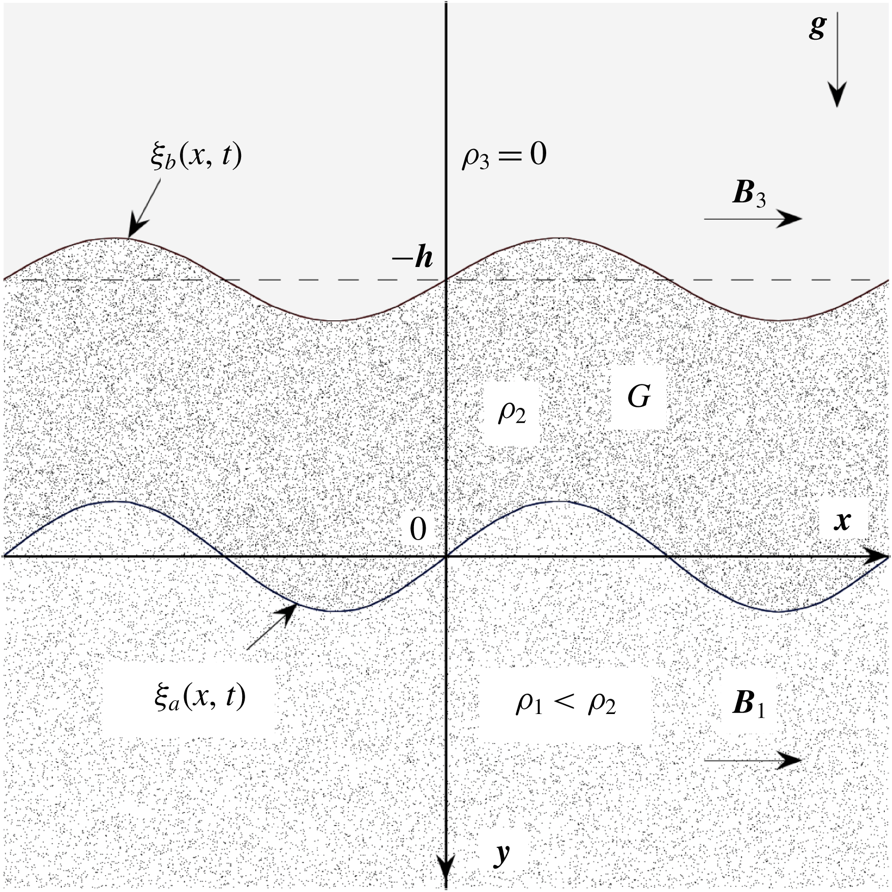
Schematic of the two-corrugated-interfaces system formed by an incompressible elastic slab with average thickness
 $h$
laying above a lighter semi-infinite incompressible ideal fluid with horizontal magnetic fields at both sides of the slab.
2 Linear MRT instability
2.1 Fundamental equations
We consider the situation of the two-dimensional system schematically described in figure 1, in which a Hookean medium of thickness
 $h$
, density
 $\unicode[STIX]{x1D70C}_{2}$
and shear modulus
 $G$
occupies the magnetic-field-free region
 $-h\leqslant y\leqslant 0$
. The slab overlays an ideal fluid of density
 $\unicode[STIX]{x1D70C}_{1}<\unicode[STIX]{x1D70C}_{2}$
occupying the region
 $y\geqslant 0$
, which is filled with a uniform magnetic field
 $\boldsymbol{B}_{\mathbf{1}}=B_{1}\boldsymbol{e}_{\boldsymbol{x}}$
(
 $\boldsymbol{e}_{\boldsymbol{x}}$
is the unitary vector in the direction of the
 $x$
-axis). In the region over the slab,
 $y\leqslant -h$
, we assume a medium with density
 $\unicode[STIX]{x1D70C}_{3}=0$
(physically, it would be a tenuous ideal medium such that
 $\unicode[STIX]{x1D70C}_{3}\ll \unicode[STIX]{x1D70C}_{2}$
,
 $\unicode[STIX]{x1D70C}_{1}$
) that is also filled with a uniform magnetic field
 $\boldsymbol{B}_{\mathbf{3}}=B_{3}\boldsymbol{e}_{\boldsymbol{x}}$
. The whole system is under the action of the uniform gravity acceleration field
 $\boldsymbol{g}=g\boldsymbol{e}_{\boldsymbol{y}}=-\unicode[STIX]{x1D735}\unicode[STIX]{x1D711}$
(
 $\boldsymbol{e}_{\boldsymbol{y}}$
is the unitary vector in the vertical direction and
 $\unicode[STIX]{x1D711}$
is the gravitational potential). In each region we consider that the medium is incompressible and perfectly conducting, and that there are no free charges. The media are also considered to be immiscible.
We start the analysis of the MRT instability with the equations for mass and momentum conservation in the following general form:
 $$\begin{eqnarray}\displaystyle & \displaystyle {\displaystyle \frac{\text{d}\unicode[STIX]{x1D70C}_{n}}{\text{d}t}}+\unicode[STIX]{x1D70C}_{n}{\displaystyle \frac{\unicode[STIX]{x2202}v_{ni}}{\unicode[STIX]{x2202}x_{i}}}=0, & \displaystyle\end{eqnarray}$$
 $$\begin{eqnarray}\displaystyle & \displaystyle \unicode[STIX]{x1D70C}_{n}{\displaystyle \frac{\text{d}v_{ni}}{\text{d}t}}=-{\displaystyle \frac{\unicode[STIX]{x2202}p_{n}}{\unicode[STIX]{x2202}x_{i}}}+\unicode[STIX]{x1D70C}_{n}g\unicode[STIX]{x1D6FF}_{iy}+{\displaystyle \frac{\unicode[STIX]{x2202}\unicode[STIX]{x1D70E}_{ik}^{(n)}}{\unicode[STIX]{x2202}x_{k}}}+\unicode[STIX]{x1D716}_{ijk}J_{nj}B_{nk}, & \displaystyle\end{eqnarray}$$
where
 $n=1,2,3$
refer, respectively, to the bottom, middle and top regions, and we have used index notation for Cartesian vectors and tensors so that
 $i=1,2,3$
indicate the space coordinates
 $x$
,
 $y$
,
 $z$
. Furthermore
 $\unicode[STIX]{x1D716}_{ijk}$
is the Levi-Civita pseudo-tensor (
 $\unicode[STIX]{x1D716}_{ijk}J_{nj}B_{nk}=(\boldsymbol{J}_{\boldsymbol{n}}\times \boldsymbol{B}_{\boldsymbol{n}})_{i}$
);
 $\boldsymbol{J}_{\boldsymbol{n}}$
is the current density;
 $\boldsymbol{B}_{\boldsymbol{n}}$
is the magnetic field as defined above in the region
 $n$
;
 $v_{ni}$
,
 $\unicode[STIX]{x1D70C}_{n}$
and
 $p_{n}$
are, respectively, the
 $i$
th velocity component, density and pressure; and
 $\unicode[STIX]{x1D70E}_{ik}^{(n)}$
is the deviatoric part of the stress tensor
 $\unicode[STIX]{x1D6F4}_{ik}^{(n)}=-p_{n}\unicode[STIX]{x1D6FF}_{ik}+\unicode[STIX]{x1D70E}_{ik}^{(n)}$
of the medium
 $n$
(
 $\unicode[STIX]{x1D6FF}_{ik}$
is the Kronecker
 $\unicode[STIX]{x1D6FF}$
). We will use interchangeably vector and index notation as appropriate for the presentation of calculations. Also,
 $\text{d}\unicode[STIX]{x1D6E9}/\text{d}t$
represents the material derivative of any magnitude
 $\unicode[STIX]{x1D6E9}$
:
 $$\begin{eqnarray}\displaystyle {\displaystyle \frac{\text{d}\unicode[STIX]{x1D6E9}}{\text{d}t}}={\displaystyle \frac{\unicode[STIX]{x2202}\unicode[STIX]{x1D6E9}}{\unicode[STIX]{x2202}t}}+(\boldsymbol{v}\boldsymbol{\cdot }\unicode[STIX]{x1D735})\unicode[STIX]{x1D6E9}. & & \displaystyle\end{eqnarray}$$
The previous equations have to be complemented with the Maxwell equations. Namely, the current density
 $\boldsymbol{J}_{\boldsymbol{n}}$
is related to the magnetic field
 $\boldsymbol{B}_{\boldsymbol{n}}$
by means of Ampere’s law. In a medium with no free charges, it reads
 $$\begin{eqnarray}\displaystyle \unicode[STIX]{x1D735}\times \boldsymbol{B}_{\boldsymbol{n}}=\unicode[STIX]{x1D707}_{n}\boldsymbol{J}_{\boldsymbol{n}}, & & \displaystyle\end{eqnarray}$$
where
 $\unicode[STIX]{x1D707}_{n}$
is the magnetic permeability of the
 $n$
-medium. Then, the Lorentz force
 $\boldsymbol{F}_{\boldsymbol{L}}^{(\boldsymbol{n})}=\boldsymbol{J}_{\boldsymbol{n}}\times \boldsymbol{B}_{\boldsymbol{n}}$
is
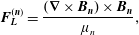 $$\begin{eqnarray}\displaystyle \boldsymbol{F}_{\boldsymbol{L}}^{(\boldsymbol{n})}={\displaystyle \frac{(\unicode[STIX]{x1D735}\times \boldsymbol{B}_{\boldsymbol{n}})\times \boldsymbol{B}_{\boldsymbol{n}}}{\unicode[STIX]{x1D707}_{n}}}, & & \displaystyle\end{eqnarray}$$
which can be written in terms of the magnetic stress tensor
 $\unicode[STIX]{x1D614}_{ik}$
by using Gauss’s law for the magnetism
 $\unicode[STIX]{x1D735}\boldsymbol{\cdot }\boldsymbol{B}_{\boldsymbol{n}}=0$
:
 $$\begin{eqnarray}\displaystyle F_{Li}^{(n)}={\displaystyle \frac{\unicode[STIX]{x2202}\unicode[STIX]{x1D614}_{ik}^{(n)}}{\unicode[STIX]{x2202}x_{k}}},\quad \unicode[STIX]{x1D614}_{ik}^{(n)}=-{\displaystyle \frac{B_{nj}B_{nj}}{2\unicode[STIX]{x1D707}_{n}}}\unicode[STIX]{x1D6FF}_{ik}+{\displaystyle \frac{B_{ni}B_{nk}}{\unicode[STIX]{x1D707}_{n}}}. & & \displaystyle\end{eqnarray}$$
On the other hand, the magnetic field
 $\boldsymbol{B}_{\boldsymbol{n}}$
is related to the material velocity
 $\boldsymbol{v}_{\boldsymbol{n}}$
through Faraday’s law:
 $$\begin{eqnarray}\displaystyle {\displaystyle \frac{\unicode[STIX]{x2202}\boldsymbol{B}_{\boldsymbol{n}}}{\unicode[STIX]{x2202}t}}=-\unicode[STIX]{x1D735}\times \boldsymbol{E}_{\boldsymbol{n}}=\unicode[STIX]{x1D735}\times (\boldsymbol{v}_{\boldsymbol{n}}\times \boldsymbol{B}_{\boldsymbol{n}}), & & \displaystyle\end{eqnarray}$$
where we have taken into account Ohm’s law
 $\boldsymbol{J}_{\boldsymbol{n}}=\unicode[STIX]{x1D702}_{n}(\boldsymbol{E}_{\boldsymbol{n}}+\boldsymbol{v}_{\boldsymbol{n}}\times \boldsymbol{B}_{\boldsymbol{n}})$
(
 $\unicode[STIX]{x1D702}_{n}$
is the electrical conductivity) for media with very high conductivity (
 $\unicode[STIX]{x1D702}_{n}\rightarrow \infty$
) or with
 $\boldsymbol{J}_{\boldsymbol{n}}=0$
, so that we have
 $\boldsymbol{E}_{\boldsymbol{n}}=-\boldsymbol{v}_{\boldsymbol{n}}\times \boldsymbol{B}_{\boldsymbol{n}}$
. The previous equation can also be written in the following alternative form:
 $$\begin{eqnarray}\displaystyle {\displaystyle \frac{\text{d}B_{ni}}{\text{d}t}}={\displaystyle \frac{\unicode[STIX]{x2202}v_{ni}}{\unicode[STIX]{x2202}x_{j}}}B_{nj}, & & \displaystyle\end{eqnarray}$$
which shows that the magnetic field is ‘frozen’ in the fluid and it moves as a material substance (Chandrasekhar Reference Chandrasekhar1961).
From (2.6b ), the momentum conservation equation (2.2) can be rewritten in a more symmetric form as follows:
 $$\begin{eqnarray}\displaystyle \unicode[STIX]{x1D70C}_{n}{\displaystyle \frac{\text{d}v_{ni}}{\text{d}t}}=-{\displaystyle \frac{\unicode[STIX]{x2202}p_{n}}{\unicode[STIX]{x2202}x_{i}}}+\unicode[STIX]{x1D70C}_{n}g\unicode[STIX]{x1D6FF}_{iy}+{\displaystyle \frac{\unicode[STIX]{x2202}(\unicode[STIX]{x1D70E}_{ik}^{(n)}+\unicode[STIX]{x1D614}_{ik}^{(n)})}{\unicode[STIX]{x2202}x_{k}}}. & & \displaystyle\end{eqnarray}$$
In addition, for a Hookean medium,
 $\unicode[STIX]{x1D70E}_{ik}^{(n)}$
is given by the following expression:
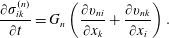 $$\begin{eqnarray}\displaystyle {\displaystyle \frac{\unicode[STIX]{x2202}\unicode[STIX]{x1D70E}_{ik}^{(n)}}{\unicode[STIX]{x2202}t}}=G_{n}\left({\displaystyle \frac{\unicode[STIX]{x2202}v_{ni}}{\unicode[STIX]{x2202}x_{k}}}+{\displaystyle \frac{\unicode[STIX]{x2202}v_{nk}}{\unicode[STIX]{x2202}x_{i}}}\right). & & \displaystyle\end{eqnarray}$$
Then, we can solve the linear stability problem by considering small-amplitude perturbations about the solution for a flat slab. Since in equilibrium the deviatoric part of the stress tensor vanishes, and we are assuming an incompressible medium, we obtain the following hydrostatic solution:
 $$\begin{eqnarray}\displaystyle p(y)=\left\{\begin{array}{@{}ll@{}}0 & y\leqslant -h,\\[2.0pt] {\displaystyle \frac{B_{3}^{2}}{2\unicode[STIX]{x1D707}_{3}}}+\unicode[STIX]{x1D70C}_{2}g(y+h) & -h\leqslant y\leqslant 0,\\[10.0pt] p_{1}+\unicode[STIX]{x1D70C}_{1}gy & y\geqslant 0,\end{array}\right. & & \displaystyle\end{eqnarray}$$
where
 $p_{1}=\unicode[STIX]{x1D70C}_{2}gh+(B_{3}^{2}/2\unicode[STIX]{x1D707}_{3})-(B_{1}^{2}/2\unicode[STIX]{x1D707}_{1})$
.
In order to close the problem we need to impose the boundary conditions corresponding to our physical situation in which the top surface of the linear elastic slab is a free surface in contact with an empty region filled with the horizontal uniform magnetic field
 $\boldsymbol{B}_{\mathbf{3}}$
, while the bottom surface is in contact with an ideal fluid which is embedded in the uniform magnetic field
 $\boldsymbol{B}_{\mathbf{1}}$
. Integrations of (2.1) and (2.9) along the vertical coordinate
 $y$
, across the bottom and the top interfaces, respectively, yield the following jump conditions representing the continuity of the normal velocities, and of the normal and tangential stresses at such interfaces:
 $$\begin{eqnarray}\displaystyle & \displaystyle \Vert -p_{n}\unicode[STIX]{x1D6FF}_{ik}+\unicode[STIX]{x1D70E}_{ik}^{(n)}n_{k}+\unicode[STIX]{x1D614}_{ik}^{(n)}n_{k}\Vert =0, & \displaystyle\end{eqnarray}$$
 $$\begin{eqnarray}\displaystyle & \displaystyle \Vert -v_{ny}\Vert =0 & \displaystyle\end{eqnarray}$$
(with
 $i=y$
or
 $x$
), where
 $\Vert Q\Vert =Q(y_{0}+0^{+})-Q(y_{0}-0^{+})$
, with
 $y_{0}=0$
or
 $y_{0}=-h$
, and
 $0^{+}\rightarrow 0$
.
2.2 Linearised equations
In order to linearise the previous set of equations we express every magnitude
 $\unicode[STIX]{x1D6E9}$
as
 $\unicode[STIX]{x1D6E9}=\unicode[STIX]{x1D6E9}_{0}+\unicode[STIX]{x1D6FF}\unicode[STIX]{x1D6E9}$
, where
 $\unicode[STIX]{x1D6E9}_{0}$
and
 $\unicode[STIX]{x1D6FF}\unicode[STIX]{x1D6E9}\ll \unicode[STIX]{x1D6E9}_{0}$
are, respectively, the equilibrium value of the magnitude and its perturbation. Then, by considering incompressible perturbations (
 $\unicode[STIX]{x1D6FF}\unicode[STIX]{x1D70C}_{n}=0$
), we get the linearised equations for momentum and mass conservation:
 $$\begin{eqnarray}\displaystyle & \displaystyle \unicode[STIX]{x1D70C}_{n}{\displaystyle \frac{\unicode[STIX]{x2202}(\unicode[STIX]{x1D6FF}v_{ni})}{\unicode[STIX]{x2202}t}}=-{\displaystyle \frac{\unicode[STIX]{x2202}(\unicode[STIX]{x1D6FF}p_{n}+\unicode[STIX]{x1D70C}_{n}\unicode[STIX]{x1D6FF}\unicode[STIX]{x1D711}_{n})}{\unicode[STIX]{x2202}x_{i}}}+{\displaystyle \frac{\unicode[STIX]{x2202}(\unicode[STIX]{x1D61A}_{ik}^{(n)}+\unicode[STIX]{x1D61B}_{ik}^{(n)})}{\unicode[STIX]{x2202}x_{k}}}, & \displaystyle\end{eqnarray}$$
 $$\begin{eqnarray}\displaystyle & \displaystyle {\displaystyle \frac{\unicode[STIX]{x2202}(\unicode[STIX]{x1D6FF}v_{ni})}{\unicode[STIX]{x2202}x_{i}}}=0, & \displaystyle\end{eqnarray}$$
where for simplicity we have defined
 $\unicode[STIX]{x1D6FF}\unicode[STIX]{x1D70E}_{ik}^{(n)}\equiv \unicode[STIX]{x1D61A}_{ik}^{(n)}$
,
 $\unicode[STIX]{x1D6FF}\unicode[STIX]{x1D614}_{ik}^{(n)}\equiv \unicode[STIX]{x1D61B}_{ik}^{(n)}$
, and they are given, respectively, by the following relationships:
 $$\begin{eqnarray}\displaystyle & \displaystyle {\displaystyle \frac{\unicode[STIX]{x2202}\unicode[STIX]{x1D61A}_{ik}^{(n)}}{\unicode[STIX]{x2202}t}}=G_{n}\left[{\displaystyle \frac{\unicode[STIX]{x2202}(\unicode[STIX]{x1D6FF}v_{ni})}{\unicode[STIX]{x2202}x_{k}}}+{\displaystyle \frac{\unicode[STIX]{x2202}(\unicode[STIX]{x1D6FF}v_{nk})}{\unicode[STIX]{x2202}x_{i}}}\right], & \displaystyle\end{eqnarray}$$
 $$\begin{eqnarray}\displaystyle & \displaystyle \unicode[STIX]{x1D61B}_{ik}^{(n)}=-{\displaystyle \frac{B_{nj}\unicode[STIX]{x1D6FF}B_{nj}}{\unicode[STIX]{x1D707}_{n}}}\unicode[STIX]{x1D6FF}_{ik}+{\displaystyle \frac{B_{ni}\unicode[STIX]{x1D6FF}B_{nk}}{\unicode[STIX]{x1D707}_{n}}}+{\displaystyle \frac{B_{nk}\unicode[STIX]{x1D6FF}B_{ni}}{\unicode[STIX]{x1D707}_{n}}}, & \displaystyle\end{eqnarray}$$
where the magnetic field perturbation turns out from (2.7) or (2.8):
 $$\begin{eqnarray}\displaystyle {\displaystyle \frac{\unicode[STIX]{x2202}(\unicode[STIX]{x1D6FF}B_{ni})}{\unicode[STIX]{x2202}t}}=B_{nk}{\displaystyle \frac{\unicode[STIX]{x2202}(\unicode[STIX]{x1D6FF}v_{ni})}{\unicode[STIX]{x2202}x_{k}}}. & & \displaystyle\end{eqnarray}$$
For the present case (2.17) can be rewritten by taking into account that
 $B_{nj}=B_{n}\unicode[STIX]{x1D6FF}_{jx}$
:
 $$\begin{eqnarray}\displaystyle \unicode[STIX]{x1D61B}_{ik}^{(n)}={\displaystyle \frac{B_{n}}{\unicode[STIX]{x1D707}_{n}}}(-\unicode[STIX]{x1D6FF}B_{nx}\unicode[STIX]{x1D6FF}_{ik}+\unicode[STIX]{x1D6FF}B_{nk}\unicode[STIX]{x1D6FF}_{ix}+\unicode[STIX]{x1D6FF}B_{ni}\unicode[STIX]{x1D6FF}_{kx}). & & \displaystyle\end{eqnarray}$$
To obtain suitable equations for the description of the perturbed velocity field, we use the Helmholtz decomposition (Lamb Reference Lamb1945, Eringen & Susuhi Reference Eringen and Susuhi1975, Menikoff et al.
Reference Menikoff, Mjolness, Sharp, Zemach and Doyle1978, Thorne & Blandford Reference Thorne and Blandford2017) whereby the velocity field can be written as the sum of an irrotational part plus a solenoidal part, in terms of the scalar potential
 $\unicode[STIX]{x1D719}_{n}$
and the vector potential
 $\unicode[STIX]{x1D74D}_{\boldsymbol{n}}$
, which for the two-dimensional perturbation we consider here will be written as
 $\unicode[STIX]{x1D74D}_{\boldsymbol{n}}=\unicode[STIX]{x1D713}_{n}\boldsymbol{e}_{\boldsymbol{z}}$
(
 $\boldsymbol{e}_{\boldsymbol{z}}$
is the unitary vector in the direction of the
 $z$
-axis). Therefore, we have
 $$\begin{eqnarray}\displaystyle \unicode[STIX]{x1D6FF}\boldsymbol{v}_{\boldsymbol{n}}=\unicode[STIX]{x1D735}\unicode[STIX]{x1D719}_{n}+\unicode[STIX]{x1D735}\times (\unicode[STIX]{x1D713}_{n}\boldsymbol{e}_{\boldsymbol{z}}). & & \displaystyle\end{eqnarray}$$
By introducing (2.20) into (2.14) and (2.15), we get
 $$\begin{eqnarray}\displaystyle & \displaystyle \unicode[STIX]{x1D735}\left\{{\displaystyle \frac{\unicode[STIX]{x2202}}{\unicode[STIX]{x2202}t}}\left(\unicode[STIX]{x1D70C}_{n}{\displaystyle \frac{\unicode[STIX]{x2202}\unicode[STIX]{x1D719}_{n}}{\unicode[STIX]{x2202}t}}+\unicode[STIX]{x1D6FF}p_{n}+\unicode[STIX]{x1D70C}_{n}\unicode[STIX]{x1D6FF}\unicode[STIX]{x1D711}_{n}\right)+{\displaystyle \frac{B_{n}^{2}}{\unicode[STIX]{x1D707}_{n}}}\left[{\displaystyle \frac{\unicode[STIX]{x2202}(\unicode[STIX]{x1D6FF}v_{nx})}{\unicode[STIX]{x2202}x}}-{\displaystyle \frac{\unicode[STIX]{x2202}^{2}\unicode[STIX]{x1D719}_{n}}{\unicode[STIX]{x2202}x^{2}}}\right]\right\} & \displaystyle \nonumber\\ \displaystyle & \quad +\,\unicode[STIX]{x1D735}\times \left[\left(\unicode[STIX]{x1D70C}_{n}{\displaystyle \frac{\unicode[STIX]{x2202}^{2}\unicode[STIX]{x1D713}_{n}}{\unicode[STIX]{x2202}t^{2}}}-G_{n}\unicode[STIX]{x1D6FB}^{2}\unicode[STIX]{x1D713}_{n}-{\displaystyle \frac{B_{n}^{2}}{\unicode[STIX]{x1D707}_{n}}}{\displaystyle \frac{\unicode[STIX]{x2202}^{2}\unicode[STIX]{x1D713}_{n}}{\unicode[STIX]{x2202}x^{2}}}\right)\boldsymbol{e}_{\boldsymbol{z}}\right]=0, & \displaystyle\end{eqnarray}$$
 $$\begin{eqnarray}\displaystyle & \displaystyle \unicode[STIX]{x1D6FB}^{2}\unicode[STIX]{x1D719}_{n}=0. & \displaystyle\end{eqnarray}$$
In our present problem,
 $G_{1}=G_{3}=0$
,
 $G_{2}\equiv G$
and
 $\boldsymbol{B}_{\mathbf{2}}=0$
, so that the second term of (2.21) is equal to zero. Then, by using the so-called Bernoulli gauge (Lamb Reference Lamb1945, Menikoff et al.
Reference Menikoff, Mjolness, Sharp, Zemach and Doyle1978, Thorne & Blandford Reference Thorne and Blandford2017), we can choose
 $\unicode[STIX]{x1D719}_{n}$
and
 $\unicode[STIX]{x1D713}_{n}$
as solutions of the following system of equations:
 $$\begin{eqnarray}\displaystyle \unicode[STIX]{x1D6FE}\unicode[STIX]{x1D719}_{n}+{\displaystyle \frac{\unicode[STIX]{x1D6FF}p_{n}}{\unicode[STIX]{x1D70C}_{n}}}+\unicode[STIX]{x1D6FF}\unicode[STIX]{x1D711}_{n}=0,\quad \unicode[STIX]{x1D6FB}^{2}\unicode[STIX]{x1D719}_{n}=0, & & \displaystyle\end{eqnarray}$$
 $$\begin{eqnarray}\displaystyle \unicode[STIX]{x1D713}_{1}=\unicode[STIX]{x1D713}_{3}=0,\quad \unicode[STIX]{x1D6FE}^{2}\unicode[STIX]{x1D713}_{2}={\displaystyle \frac{G}{\unicode[STIX]{x1D70C}_{2}}}\unicode[STIX]{x1D6FB}^{2}\unicode[STIX]{x1D713}_{2}, & & \displaystyle\end{eqnarray}$$
where
 $\unicode[STIX]{x1D6FF}\unicode[STIX]{x1D711}_{n}=-g\unicode[STIX]{x1D6FF}v_{ny}/\unicode[STIX]{x1D6FE}$
,
 $\unicode[STIX]{x1D6FE}$
is the asymptotic instability growth rate and we have taken two-dimensional perturbations of the form
 $$\begin{eqnarray}\displaystyle & \displaystyle \unicode[STIX]{x1D719}_{n}\propto \text{e}^{(\unicode[STIX]{x1D6FE}t+qy)}\sin kx, & \displaystyle\end{eqnarray}$$
 $$\begin{eqnarray}\displaystyle & \displaystyle \unicode[STIX]{x1D713}_{2}\propto \text{e}^{(\unicode[STIX]{x1D6FE}t+q^{\prime }y)}\cos kx. & \displaystyle\end{eqnarray}$$
In addition, consistently with (2.23b ) and (2.24b ):
 $$\begin{eqnarray}\displaystyle q=\pm k,\quad q^{\prime }=\pm \unicode[STIX]{x1D706},\quad \unicode[STIX]{x1D706}=\sqrt{k^{2}+{\displaystyle \frac{\unicode[STIX]{x1D6FE}^{2}\unicode[STIX]{x1D70C}_{2}}{G}}}. & & \displaystyle\end{eqnarray}$$
On the other hand, perturbations of the deviatoric stress tensor
 $\unicode[STIX]{x1D61A}_{ik}^{(2)}$
, of the magnetic stress tensors
 $\unicode[STIX]{x1D61B}_{ik}^{(n)}$
and of the magnetic fields
 $\unicode[STIX]{x1D6FF}B_{ni}$
are given by (2.16), (2.17) and (2.18), respectively. Similarly, the velocity field is obtained from (2.20):
 $$\begin{eqnarray}\displaystyle \unicode[STIX]{x1D6FF}v_{nx}={\displaystyle \frac{\unicode[STIX]{x2202}\unicode[STIX]{x1D719}_{n}}{\unicode[STIX]{x2202}x}}+{\displaystyle \frac{\unicode[STIX]{x2202}\unicode[STIX]{x1D713}_{n}}{\unicode[STIX]{x2202}y}},\quad \unicode[STIX]{x1D6FF}v_{ny}={\displaystyle \frac{\unicode[STIX]{x2202}\unicode[STIX]{x1D719}_{n}}{\unicode[STIX]{x2202}y}}-{\displaystyle \frac{\unicode[STIX]{x2202}\unicode[STIX]{x1D713}_{n}}{\unicode[STIX]{x2202}x}}. & & \displaystyle\end{eqnarray}$$
On the other hand, the linearised boundary conditions at each interface are
 $$\begin{eqnarray}\displaystyle & \displaystyle \Vert -\unicode[STIX]{x1D6FF}p_{n}\unicode[STIX]{x1D6FF}_{ik}+\unicode[STIX]{x1D61A}_{ik}^{(n)}n_{k}+\unicode[STIX]{x1D61B}_{ik}^{(n)}n_{k}\Vert =0, & \displaystyle\end{eqnarray}$$
 $$\begin{eqnarray}\displaystyle & \displaystyle \Vert -\unicode[STIX]{x1D6FF}v_{ny}\Vert =0 & \displaystyle\end{eqnarray}$$
(with
 $i=y$
or
 $x$
), where
 $\Vert Q\Vert =Q(y_{0}+0^{+})-Q(y_{0}-0^{+})$
(with
 $y_{0}=\unicode[STIX]{x1D709}_{a}$
or
 $y_{0}=-h+\unicode[STIX]{x1D709}_{b}$
, where
 $0^{+}\rightarrow 0$
, and
 $\unicode[STIX]{x1D709}_{a}=\unicode[STIX]{x1D709}_{a}(x,t)$
and
 $\unicode[STIX]{x1D709}_{b}=\unicode[STIX]{x1D709}_{b}(x,t)$
are the perturbation amplitudes of the bottom and top interfaces, respectively), and we have to take into account that both
 $\unicode[STIX]{x1D61A}_{ik}^{(n)}$
and
 $\unicode[STIX]{x1D61B}_{ik}^{(n)}$
are symmetric tensors. By taking into account that in the linear regime we are considering
 $n_{x}=\unicode[STIX]{x2202}\unicode[STIX]{x1D709}_{a,b}/\unicode[STIX]{x2202}x\sim k\unicode[STIX]{x1D709}_{a,b}\ll 1$
and
 $n_{y}\sim 1$
, we can rewrite (2.29) as follows:
 $$\begin{eqnarray}\displaystyle \Vert -\unicode[STIX]{x1D6FF}p_{n}\unicode[STIX]{x1D6FF}_{yi}+\unicode[STIX]{x1D61A}_{yi}^{(n)}+\unicode[STIX]{x1D61B}_{yi}^{(n)}\Vert =0. & & \displaystyle\end{eqnarray}$$
Therefore, the required boundary conditions read
 $$\begin{eqnarray}\displaystyle \unicode[STIX]{x1D6FF}v_{1y}(0)=\unicode[STIX]{x1D6FF}v_{2y}(0)=\unicode[STIX]{x1D6FE}\unicode[STIX]{x1D709}_{a},\quad \unicode[STIX]{x1D6FF}v_{2y}(-h)=\unicode[STIX]{x1D6FF}v_{3y}(-h)=\unicode[STIX]{x1D6FE}\unicode[STIX]{x1D709}_{b}, & & \displaystyle\end{eqnarray}$$
 $$\begin{eqnarray}\displaystyle -\unicode[STIX]{x1D6FF}p_{1}(0)+\unicode[STIX]{x1D61B}_{yy}^{(1)}(0)=-\unicode[STIX]{x1D6FF}p_{2}(0)+\unicode[STIX]{x1D61A}_{yy}^{(2)}(0),\quad -\unicode[STIX]{x1D6FF}p_{2}(-h)+\unicode[STIX]{x1D61A}_{yy}^{(2)}(-h)=\unicode[STIX]{x1D61B}_{yy}^{(3)}(-h), & & \displaystyle \nonumber\\ \displaystyle & & \displaystyle\end{eqnarray}$$
 $$\begin{eqnarray}\displaystyle \unicode[STIX]{x1D61B}_{xy}^{(1)}(0)=\unicode[STIX]{x1D61A}_{xy}^{(2)}(0),\quad \unicode[STIX]{x1D61A}_{xy}^{(2)}(-h)=\unicode[STIX]{x1D61B}_{xy}^{(3)}(-h), & & \displaystyle\end{eqnarray}$$
where
 $\unicode[STIX]{x1D61A}_{ik}^{(2)}$
is obtained from (2.16),
 $\unicode[STIX]{x1D61B}_{ik}^{(n)}$
is obtained from (2.17) and (2.18) and
 $\unicode[STIX]{x1D6FF}p_{n}$
is given by (2.23a
):
 $$\begin{eqnarray}\displaystyle -\unicode[STIX]{x1D6FF}p_{n}=-\unicode[STIX]{x1D70C}_{n}g{\displaystyle \frac{\unicode[STIX]{x1D6FF}v_{ny}}{\unicode[STIX]{x1D6FE}}}+\unicode[STIX]{x1D70C}_{n}\unicode[STIX]{x1D6FE}\unicode[STIX]{x1D719}_{n}. & & \displaystyle\end{eqnarray}$$
Before using these equations for solving the problem presented in figure 1, let us first retrieve the results of Lau et al. (Reference Lau, Zier, Rittersdorf, Weis and Gilgenbach2011) for the MRT instability in ideal media (
 $G=0$
), and consider also the case of the MRT instability in two semi-infinite (
 $h\rightarrow \infty$
) media studied by Sun & Piriz (Reference Sun and Piriz2014) in which the heaviest one is an elastic medium. Later, these cases can be used for comparisons with the present problem and to aid the physical interpretations.
3 Brief overview of some previous relevant results
3.1 Ideal fluid slab atop a lighter semi-infinite ideal fluid
In this case
 $\unicode[STIX]{x1D713}_{2}=0$
, and the velocity field is derived from the solution of the Laplace equation (2.22). The resulting velocity potentials
 $\unicode[STIX]{x1D719}_{n}$
in the corresponding regions are conveniently written in the following form:
 $$\begin{eqnarray}\displaystyle & \displaystyle \unicode[STIX]{x1D719}_{1}=a_{M1}\text{e}^{-ky}\text{e}^{\unicode[STIX]{x1D6FE}t}\sin kx\quad (y\geqslant 0), & \displaystyle\end{eqnarray}$$
 $$\begin{eqnarray}\displaystyle & \displaystyle \unicode[STIX]{x1D719}_{2}={\displaystyle \frac{a_{M2}\cosh ky+b_{M2}\cosh k(h+y)}{\sinh kh}}\text{e}^{\unicode[STIX]{x1D6FE}t}\sin kx\quad (-h\leqslant y\leqslant 0), & \displaystyle\end{eqnarray}$$
 $$\begin{eqnarray}\displaystyle & \displaystyle \unicode[STIX]{x1D719}_{3}=a_{M3}\text{e}^{k(h+y)}\text{e}^{\unicode[STIX]{x1D6FE}t}\sin kx\quad (y\leqslant -h), & \displaystyle\end{eqnarray}$$
where the constants
 $a_{Mn}$
and
 $b_{M2}$
will be determined together with the instability growth rate
 $\unicode[STIX]{x1D6FE}$
from the boundary conditions at
 $y=0$
and
 $y=-h$
given by (2.32)–(2.34). In this case, since the heavier medium (
 $n=2$
) is also ideal, we have
 $\unicode[STIX]{x1D61A}_{ik}^{(2)}=0$
, and those boundary conditions read as follows:
 $$\begin{eqnarray}\displaystyle \unicode[STIX]{x1D6FF}v_{1y}(0)=\unicode[STIX]{x1D6FF}v_{2y}(0),\quad \unicode[STIX]{x1D6FF}v_{2y}(-h)=\unicode[STIX]{x1D6FF}v_{3y}(-h), & & \displaystyle\end{eqnarray}$$
 $$\begin{eqnarray}\displaystyle -\unicode[STIX]{x1D6FF}p_{1}(0)+\unicode[STIX]{x1D61B}_{yy}^{(1)}(0)=-\unicode[STIX]{x1D6FF}p_{2}(0),\quad -\unicode[STIX]{x1D6FF}p_{2}(-h)=-\unicode[STIX]{x1D6FF}p_{3}(-h)+\unicode[STIX]{x1D61B}_{yy}^{(3)}(-h), & & \displaystyle\end{eqnarray}$$
where the perturbations of the magnetic tensor are given by (2.17) and (2.18):
 $$\begin{eqnarray}\displaystyle \unicode[STIX]{x1D61B}_{yy}^{(n)}={\displaystyle \frac{B_{n}^{2}k^{2}}{\unicode[STIX]{x1D6FE}\unicode[STIX]{x1D707}_{n}}}a_{Mn}. & & \displaystyle\end{eqnarray}$$
Then, (3.4) and (3.5) produce the following set of equations:
 $$\begin{eqnarray}\displaystyle a_{M1}=-b_{M2},\quad a_{M2}=-a_{M3}, & & \displaystyle\end{eqnarray}$$
 $$\begin{eqnarray}\displaystyle & \displaystyle \unicode[STIX]{x1D6FE}\unicode[STIX]{x1D70C}_{2}\left({\displaystyle \frac{a_{M2}}{\sinh kh}}+b_{M2}\coth kh\right)-{\displaystyle \frac{\unicode[STIX]{x1D70C}_{2}kg}{\unicode[STIX]{x1D6FE}}}b_{M2}=\unicode[STIX]{x1D70C}_{1}\left(\unicode[STIX]{x1D6FE}+{\displaystyle \frac{kg}{\unicode[STIX]{x1D6FE}}}\right)a_{M1}+{\displaystyle \frac{B_{1}^{2}k^{2}}{\unicode[STIX]{x1D6FE}\unicode[STIX]{x1D707}_{1}}}a_{M1}, & \displaystyle\end{eqnarray}$$
 $$\begin{eqnarray}\displaystyle & \displaystyle \unicode[STIX]{x1D6FE}\unicode[STIX]{x1D70C}_{2}\left(a_{M2}\coth kh+{\displaystyle \frac{b_{M2}}{\sinh kh}}\right)+{\displaystyle \frac{\unicode[STIX]{x1D70C}_{2}kg}{\unicode[STIX]{x1D6FE}}}a_{M2}={\displaystyle \frac{B_{3}^{2}k^{2}}{\unicode[STIX]{x1D6FE}\unicode[STIX]{x1D707}_{3}}}a_{M3}. & \displaystyle\end{eqnarray}$$
The solution of this system yields the dispersion relation for the growth rate
 $\unicode[STIX]{x1D6FE}$
:
 $$\begin{eqnarray}\displaystyle & & \displaystyle \displaystyle \unicode[STIX]{x1D6FE}^{4}\left(1+{\displaystyle \frac{\unicode[STIX]{x1D70C}_{1}}{\unicode[STIX]{x1D70C}_{2}}}\coth kh\right)\nonumber\\ \displaystyle & & \displaystyle \displaystyle \quad +\,\unicode[STIX]{x1D6FE}^{2}\left\{{\displaystyle \frac{2k^{2}}{\unicode[STIX]{x1D70C}_{2}}}(G_{M1}+G_{M3})\coth kh+{\displaystyle \frac{\unicode[STIX]{x1D70C}_{1}}{\unicode[STIX]{x1D70C}_{2}}}\left[{\displaystyle \frac{2k^{2}}{\unicode[STIX]{x1D70C}_{2}}}G_{M3}+kg(1+\coth kh)\right]\right\}\nonumber\\ \displaystyle & & \displaystyle \displaystyle \quad -\,\left[\left(1-{\displaystyle \frac{\unicode[STIX]{x1D70C}_{1}}{\unicode[STIX]{x1D70C}_{2}}}\right)kg-{\displaystyle \frac{2k^{2}}{\unicode[STIX]{x1D70C}_{2}}}G_{M1}\right]\left(kg+{\displaystyle \frac{2k^{2}}{\unicode[STIX]{x1D70C}_{2}}}G_{M3}\right)=0,\end{eqnarray}$$
where we have used the following definition:
 $$\begin{eqnarray}\displaystyle G_{Mn}\equiv {\displaystyle \frac{B_{n}^{2}}{2\unicode[STIX]{x1D707}_{n}}}. & & \displaystyle\end{eqnarray}$$
It may be worth noticing that for
 $G_{M1}=G_{M3}=0$
, (3.10) yields the growth rate obtained by Mikaelian (Reference Mikaelian1982) and Goncharov et al. (Reference Goncharov, McKenty, Skupsky, Betti, McCrory and Cherfils-Clérouin2000) for the case of an ideal fluid slab with no magnetic fields:
 $$\begin{eqnarray}\displaystyle \unicode[STIX]{x1D6FE}=\sqrt{{\displaystyle \frac{(\unicode[STIX]{x1D70C}_{2}-\unicode[STIX]{x1D70C}_{1})kg}{\unicode[STIX]{x1D70C}_{2}+\unicode[STIX]{x1D70C}_{1}\coth kh}}}. & & \displaystyle\end{eqnarray}$$
Later, this result will be useful for comparisons.
For the analysis of the dispersion relation (3.10) it is convenient to introduce the following dimensionless magnitudes:
 $$\begin{eqnarray}\displaystyle \unicode[STIX]{x1D705}_{M}={\displaystyle \frac{k}{k_{0M}}},\quad \unicode[STIX]{x1D70E}_{M}={\displaystyle \frac{\unicode[STIX]{x1D6FE}}{\sqrt{k_{0M}g}}},\quad k_{0M}={\displaystyle \frac{\unicode[STIX]{x1D70C}_{2}g}{G_{M1}}}. & & \displaystyle\end{eqnarray}$$
Then, we get
 $$\begin{eqnarray}\displaystyle & & \displaystyle \displaystyle \unicode[STIX]{x1D70E}_{M}^{4}\left(1+{\displaystyle \frac{1-A_{T}}{1+A_{T}}}\coth \unicode[STIX]{x1D6FC}_{M}\unicode[STIX]{x1D705}_{M}\right)\nonumber\\ \displaystyle & & \displaystyle \displaystyle \quad +\,\unicode[STIX]{x1D70E}_{M}^{2}\left\{2(1+\unicode[STIX]{x1D6FD}_{M})\unicode[STIX]{x1D705}_{M}^{2}\coth \unicode[STIX]{x1D6FC}_{M}\unicode[STIX]{x1D705}_{M}+{\displaystyle \frac{1-A_{T}}{1+A_{T}}}[2\unicode[STIX]{x1D6FD}_{M}\unicode[STIX]{x1D705}_{M}^{2}+\unicode[STIX]{x1D705}_{M}(1+\coth \unicode[STIX]{x1D6FC}_{M}\unicode[STIX]{x1D705}_{M})]\right\}\nonumber\\ \displaystyle & & \displaystyle \displaystyle \quad -\,2\unicode[STIX]{x1D705}_{M}^{2}\left({\displaystyle \frac{A_{T}}{1+A_{T}}}-\unicode[STIX]{x1D705}_{M}\right)(1+2\unicode[STIX]{x1D6FD}_{M}\unicode[STIX]{x1D705}_{M})=0,\end{eqnarray}$$
where
 $$\begin{eqnarray}\displaystyle \unicode[STIX]{x1D6FD}_{M}={\displaystyle \frac{G_{M3}}{G_{M1}}},\quad \unicode[STIX]{x1D6FC}_{M}=k_{0M}h,\quad A_{T}={\displaystyle \frac{\unicode[STIX]{x1D70C}_{2}-\unicode[STIX]{x1D70C}_{1}}{\unicode[STIX]{x1D70C}_{2}+\unicode[STIX]{x1D70C}_{1}}}, & & \displaystyle\end{eqnarray}$$
and
 $A_{T}$
is the Atwood number. We have presented the dispersion relation (3.14) in a somewhat different manner from Lau et al. (Reference Lau, Zier, Rittersdorf, Weis and Gilgenbach2011), which is more suitable for our present purposes. The dimensionless growth rate
 $\unicode[STIX]{x1D70E}_{M}$
is shown in figure 2 for two values of the Atwood number (
 $A_{T}=1$
and 0.3), for three values of the ratio
 $\unicode[STIX]{x1D6FD}_{M}=G_{M3}/G_{M1}$
between the magnetic pressures above and below the dense layer, and for different values of its dimensionless thickness
 $\unicode[STIX]{x1D6FC}_{M}$
indicated by the labels on the curves.
Ideal MRT instability. Dimensionless growth rate
 $\unicode[STIX]{x1D70E}_{M}=\unicode[STIX]{x1D6FE}/\sqrt{k_{0M}g}$
as a function of the dimensionless wavenumber
 $\unicode[STIX]{x1D705}_{M}=k/k_{0M}$
(
 $k_{0M}=\unicode[STIX]{x1D70C}_{2}g/G_{M1}$
, and
 $G_{Mn}=B_{n}^{2}/(2\unicode[STIX]{x1D707}_{n})$
), for two Atwood numbers (
 $A_{T}=1$
and
 $A_{T}=0.3$
), and for three typical cases in which, respectively, the bottom magnetic field dominates (a,d), both fields are equal (b,e) and the top magnetic field dominates (c,f), and for different values of the dimensionless thickness
 $\unicode[STIX]{x1D6FC}_{M}$
(indicated by the labels on the curves).
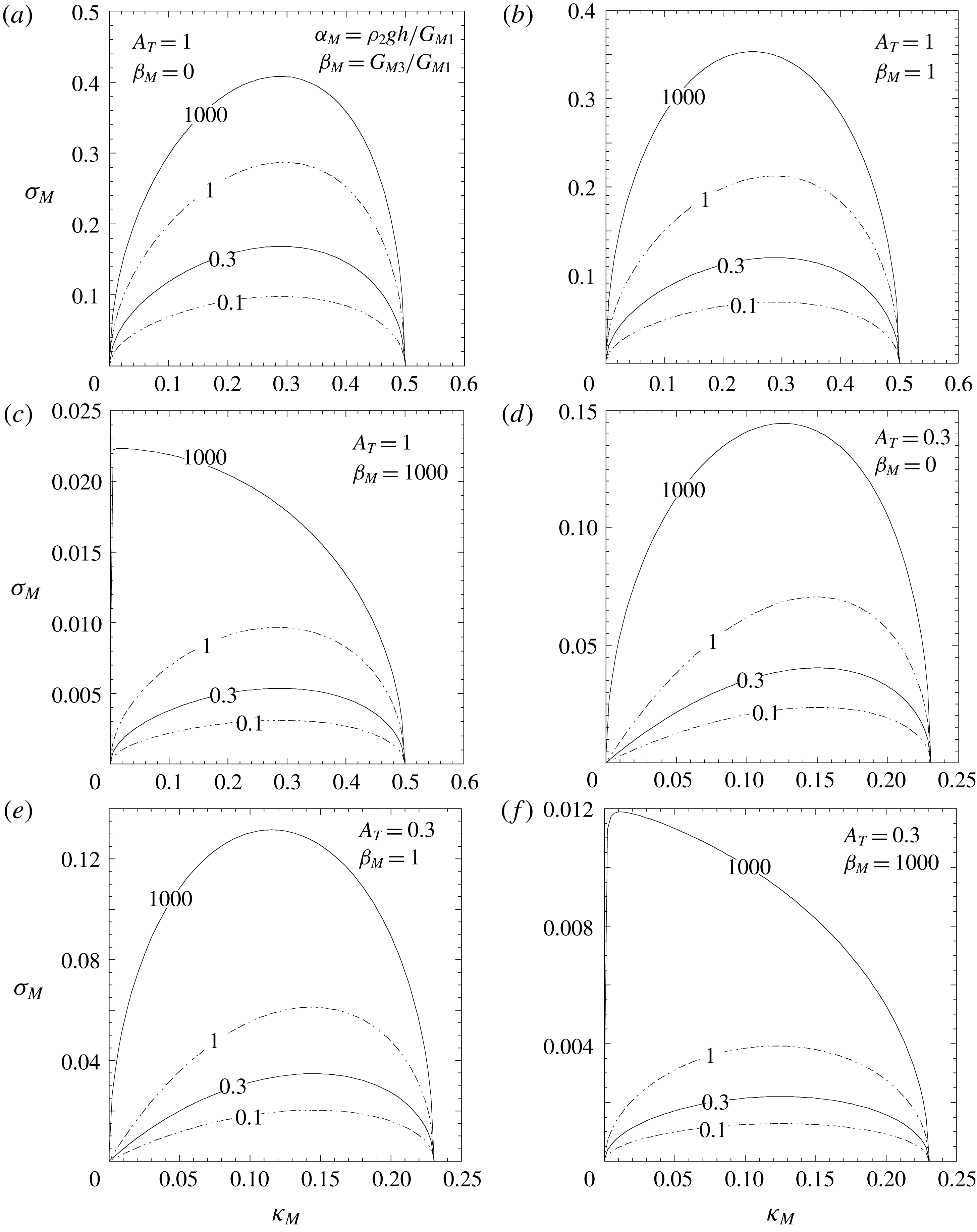
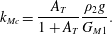
Three features have to be noticed that will be worth comparing later on with the results involving an elastic slab in § 4. Firstly, the cut-off wavenumber
 $k_{Mc}$
is independent of the slab thickness and it is determined only by the magnetic pressure
 $G_{M1}=B_{1}^{2}/(2\unicode[STIX]{x1D707}_{1})$
acting on the bottom surface of the slab:
 $$\begin{eqnarray}\displaystyle k_{Mc}={\displaystyle \frac{A_{T}}{1+A_{T}}}{\displaystyle \frac{\unicode[STIX]{x1D70C}_{2}g}{G_{M1}}}. & & \displaystyle\end{eqnarray}$$
Secondly, the maximum growth rate is smaller for the thinner slabs, and this is true for all values of
 $A_{T}$
, whereas, as shown by (3.12), when no magnetic fields are present the thinner slabs are more stable only if
 $A_{T}\neq 1$
. As was discussed by Piriz et al. (Reference Piriz, Piriz and Tahir2018), the latter behaviour is explained by the fact that the fluid in the region
 $y\geqslant 0$
exerts a force (per unitary surface)
 $\unicode[STIX]{x1D70C}_{1}g\unicode[STIX]{x1D709}_{a}$
which opposes the slab fall, and it depends only on the bottom surface deformation
 $\unicode[STIX]{x1D709}_{a}$
. Instead, the force
 $\unicode[STIX]{x1D70C}_{2}g\unicode[STIX]{x0394}h$
driving the slab fall is given by the slab-thickness change
 $\unicode[STIX]{x0394}h=\unicode[STIX]{x1D709}_{a}-\unicode[STIX]{x1D709}_{b}$
. Therefore, since
 $\unicode[STIX]{x0394}h$
is smaller for thinner slabs, and the same force
 $\unicode[STIX]{x1D70C}_{1}g\unicode[STIX]{x1D709}_{a}$
is available to support any slab, the thicker ones are less stable. For the same reason, no reduction of the growth rate occurs for
 $A_{T}=1$
, when no fluid is present below the slab for supporting it.
However, the fact that in the presence of magnetic fields the thinner slabs turn out to be more stable even for
 $A_{T}=1$
can be explained in a similar manner. In fact, uniform magnetic fields which are known to act as a surface tension (Chandrasekhar Reference Chandrasekhar1961) resist the slab deformation to an extent that depends on the local deformations
 $\unicode[STIX]{x1D709}_{a}$
at
 $y=0$
, and
 $\unicode[STIX]{x1D709}_{b}$
at
 $y=-h$
(in (3.6) it is
 $a_{M1}/\unicode[STIX]{x1D6FE}=\unicode[STIX]{x1D709}_{a}$
and
 $a_{M3}/\unicode[STIX]{x1D6FE}=\unicode[STIX]{x1D709}_{b}$
). Instead, the weight increase of the slab is once again determined by
 $\unicode[STIX]{x0394}h=\unicode[STIX]{x1D709}_{a}-\unicode[STIX]{x1D709}_{b}$
, which is smaller for thinner slabs. The stabilising effect of the magnetic field is then more effective for the thinner slabs for any
 $A_{T}$
.
Finally, we note that for a given value of
 $A_{T}$
, the magnetic field atop the layer also acts to reduce the maximum growth rate. This means that the presence of magnetic fields at any side of the slab has a stabilising effect.
3.2 Magneto-Rayleigh–Taylor instability in semi-infinite media. An elastic medium atop an ideal fluid
In this case
 $h\rightarrow -\infty$
, and
 $\unicode[STIX]{x1D713}_{2}\neq 0$
is given by (2.24). Then, the potential functions that determine the velocity field read as follows:
 $$\begin{eqnarray}\displaystyle & \displaystyle \unicode[STIX]{x1D719}_{1}=a_{s1}\text{e}^{-ky}\text{e}^{\unicode[STIX]{x1D6FE}t}\sin kx\quad (y\geqslant 0), & \displaystyle\end{eqnarray}$$
 $$\begin{eqnarray}\displaystyle & \displaystyle \unicode[STIX]{x1D719}_{2}=a_{s2}\text{e}^{ky}\text{e}^{\unicode[STIX]{x1D6FE}t}\sin kx\quad (y\leqslant 0), & \displaystyle\end{eqnarray}$$
 $$\begin{eqnarray}\displaystyle & \displaystyle \unicode[STIX]{x1D713}_{2}=c_{s2}\text{e}^{\unicode[STIX]{x1D706}y}\text{e}^{\unicode[STIX]{x1D6FE}t}\cos kx\quad (y\leqslant 0), & \displaystyle\end{eqnarray}$$
where
 $\unicode[STIX]{x1D706}$
is given by (2.27c
).
In this case, the boundary conditions must be imposed only at
 $y=0$
. Therefore, (2.32) to (2.34) read now as follows:
 $$\begin{eqnarray}\displaystyle & \displaystyle \unicode[STIX]{x1D6FF}v_{1y}(0)=\unicode[STIX]{x1D6FF}v_{2y}(0), & \displaystyle\end{eqnarray}$$
 $$\begin{eqnarray}\displaystyle & \displaystyle -\unicode[STIX]{x1D6FF}p_{1}(0)+\unicode[STIX]{x1D61B}_{yy}^{(1)}(0)=-\unicode[STIX]{x1D6FF}p_{2}(0)+\unicode[STIX]{x1D61A}_{yy}^{(2)}(0), & \displaystyle\end{eqnarray}$$
 $$\begin{eqnarray}\displaystyle & \displaystyle \unicode[STIX]{x1D61B}_{xy}^{(1)}(0)=\unicode[STIX]{x1D61A}_{xy}^{(2)}(0). & \displaystyle\end{eqnarray}$$
These equations yield the following system for obtaining the constants
 $a_{sn}$
and
 $c_{s2}$
, and the growth rate
 $\unicode[STIX]{x1D6FE}$
:
 $$\begin{eqnarray}\displaystyle -a_{s1}=a_{s2}+c_{s2},\quad a_{s2}=-{\displaystyle \frac{[(\unicode[STIX]{x1D706}^{2}+k^{2})G-2k^{2}G_{M1}]}{2k^{2}(G-G_{M1})}}c_{s2}, & & \displaystyle\end{eqnarray}$$
 $$\begin{eqnarray}\displaystyle \unicode[STIX]{x1D70C}_{1}\left(\unicode[STIX]{x1D6FE}+{\displaystyle \frac{kg}{\unicode[STIX]{x1D6FE}}}\right)a_{s1}+{\displaystyle \frac{2G_{M1}k^{2}}{\unicode[STIX]{x1D6FE}}}a_{s1}=\unicode[STIX]{x1D70C}_{2}\unicode[STIX]{x1D6FE}a_{s2}-{\displaystyle \frac{kg}{\unicode[STIX]{x1D6FE}}}\unicode[STIX]{x1D70C}_{2}(a_{s2}+c_{s2})+{\displaystyle \frac{2G}{\unicode[STIX]{x1D6FE}}}(k^{2}a_{s2}+\unicode[STIX]{x1D706}kc_{s2}).\quad & & \displaystyle\end{eqnarray}$$
From (3.23) and (3.24) we can find the dispersion relation for the growth rate:
 $$\begin{eqnarray}\displaystyle \unicode[STIX]{x1D6FE}^{2}-A_{T}kg={\displaystyle \frac{1+A_{T}}{2}}{\displaystyle \frac{4k^{2}G}{\unicode[STIX]{x1D70C}_{2}}}\left[-1+{\displaystyle \frac{kG}{\unicode[STIX]{x1D70C}_{2}\unicode[STIX]{x1D6FE}^{2}}}\left(\sqrt{k^{2}+{\displaystyle \frac{\unicode[STIX]{x1D6FE}^{2}\unicode[STIX]{x1D70C}_{2}}{G}}}-k\right)\left(1-{\displaystyle \frac{G_{M1}}{G}}\right)\right]. & & \displaystyle\end{eqnarray}$$
Notice that by doing the transformation
 $G/\unicode[STIX]{x1D6FE}\unicode[STIX]{x1D70C}_{2}\rightarrow \unicode[STIX]{x1D708}$
in the previous equation with
 $G_{M1}=0$
we recover the growth rate given by Chandrasekhar (Reference Chandrasekhar1961) for the case of a semi-infinite viscous fluid of kinematic viscosity
 $\unicode[STIX]{x1D708}$
overlaying a semi-infinite ideal fluid (Robinson & Swegle Reference Robinson and Swegle1989).
After some straightforward algebra, (3.25) can be rewritten in the following suitable form:
 $$\begin{eqnarray}\displaystyle \unicode[STIX]{x1D6FE}^{2}-A_{T}kg=-{\displaystyle \frac{1+A_{T}}{2}}{\displaystyle \frac{4k^{2}}{\unicode[STIX]{x1D70C}_{2}}}{\displaystyle \frac{(\unicode[STIX]{x1D706}G+kG_{M1})}{\unicode[STIX]{x1D706}+k}}. & & \displaystyle\end{eqnarray}$$
In the irrotational approximation considered by Sun & Piriz (Reference Sun and Piriz2014),
 $k^{2}\gg \unicode[STIX]{x1D6FE}^{2}\unicode[STIX]{x1D70C}_{2}/G$
, and then
 $\unicode[STIX]{x1D706}\approx k$
, so that (3.26) reduces to the irrotational solution.
From (3.26) we can easily see that marginal stability (
 $\unicode[STIX]{x1D6FE}=0$
) occurs for the cut-off wavenumber
 $k_{c}$
:
 $$\begin{eqnarray}\displaystyle k_{c}={\displaystyle \frac{A_{T}}{1+A_{T}}}{\displaystyle \frac{\unicode[STIX]{x1D70C}_{2}g}{G+G_{M1}}}. & & \displaystyle\end{eqnarray}$$
As was noticed by Sun & Piriz (Reference Sun and Piriz2014), in this case magnetic pressure acts practically in the same manner as elasticity to enhance the stability of the interface, and both stabilising effects are added up.
To represent graphically the dispersion relation for this case it is more convenient to write (3.25) in dimensionless form by using the following definitions:
 $$\begin{eqnarray}\displaystyle \unicode[STIX]{x1D705}={\displaystyle \frac{k}{k_{0}}},\quad \unicode[STIX]{x1D70E}={\displaystyle \frac{\unicode[STIX]{x1D6FE}}{\sqrt{k_{0}g}}},\quad k_{0}={\displaystyle \frac{\unicode[STIX]{x1D70C}_{2}g}{G}},\quad \unicode[STIX]{x1D6FD}_{1}={\displaystyle \frac{G_{M1}}{G}}. & & \displaystyle\end{eqnarray}$$
Then, it turns out
 $$\begin{eqnarray}\displaystyle \unicode[STIX]{x1D70E}^{2}=A_{T}\unicode[STIX]{x1D705}+2(1+A_{T})\unicode[STIX]{x1D705}^{2}\left\{-1+{\displaystyle \frac{\unicode[STIX]{x1D705}}{\unicode[STIX]{x1D70E}^{2}}}\left[\sqrt{\unicode[STIX]{x1D705}^{2}+\unicode[STIX]{x1D70E}^{2}}-\unicode[STIX]{x1D705}\right](1-\unicode[STIX]{x1D6FD}_{1})\right\}. & & \displaystyle\end{eqnarray}$$
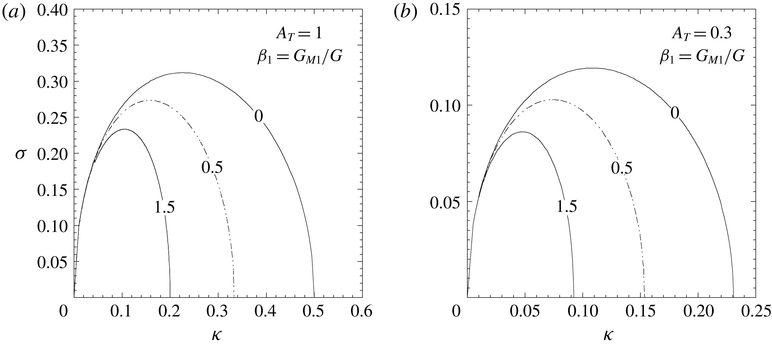
This expression is represented in figure 3 for two values of the Atwood number (
 $A_{T}=1$
and 0.3) and for three different values of the ratio
 $\unicode[STIX]{x1D6FD}_{1}$
(0, 0.5 and 1.5).
4 Elastic slab atop an ideal fluid in the presence of magnetic fields
Magneto-Rayleigh–Taylor instability in semi-infinite media with an elastic medium atop an ideal fluid. Dimensionless growth rate
 $\unicode[STIX]{x1D70E}=\unicode[STIX]{x1D6FE}/\sqrt{k_{0}g}$
as a function of the dimensionless wavenumber
 $\unicode[STIX]{x1D705}=k/k_{0}$
(
 $k_{0}=\unicode[STIX]{x1D70C}_{2}g/G$
) for three values of the ratio
 $\unicode[STIX]{x1D6FD}_{1}=G_{M1}/G$
(
 $G_{M1}=B_{1}^{2}/(2\unicode[STIX]{x1D707}_{1})$
) indicated by the labels on the curves, and for two Atwood numbers: (a)
 $A_{T}=1$
and (b)
 $A_{T}=0.3$
.
4.1 Dispersion relation
This is the case schematically represented in figure 1 in which the regions
 $y\leqslant -h$
and
 $y\geqslant 0$
are filled with uniform magnetic fields, and the elastic slab in between (
 $-h\leqslant y\leqslant 0$
) is a Hookean medium. Then
 $\unicode[STIX]{x1D713}_{2}\neq 0$
and the potential functions are conveniently written in the following form:
 $$\begin{eqnarray}\displaystyle & \displaystyle \unicode[STIX]{x1D719}_{1}=a_{1}\text{e}^{-ky}\text{e}^{\unicode[STIX]{x1D6FE}t}\sin kx\quad (y\geqslant 0), & \displaystyle\end{eqnarray}$$
 $$\begin{eqnarray}\displaystyle & \displaystyle \unicode[STIX]{x1D719}_{3}=a_{3}\text{e}^{k(h+y)}\text{e}^{\unicode[STIX]{x1D6FE}t}\sin kx\quad (y\leqslant -h), & \displaystyle\end{eqnarray}$$
 $$\begin{eqnarray}\displaystyle & \displaystyle \unicode[STIX]{x1D719}_{2}={\displaystyle \frac{a_{2}\cosh ky+b_{2}\cosh k(h+y)}{\sinh kh}}\text{e}^{\unicode[STIX]{x1D6FE}t}\sin kx\quad (-h\leqslant y\leqslant 0), & \displaystyle\end{eqnarray}$$
 $$\begin{eqnarray}\displaystyle & \displaystyle \unicode[STIX]{x1D713}_{2}={\displaystyle \frac{c_{2}\sinh \unicode[STIX]{x1D706}y+d_{2}\sinh \unicode[STIX]{x1D706}(h+y)}{\sinh \unicode[STIX]{x1D706}h}}\text{e}^{\unicode[STIX]{x1D6FE}t}\cos kx\quad (-h\leqslant y\leqslant 0), & \displaystyle\end{eqnarray}$$
and the velocity field is calculated from (2.28).
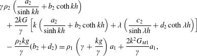
The required boundary conditions are those ones given by (2.32) to (2.34). These six boundary conditions produce the following system of linear equations:
 $$\begin{eqnarray}\displaystyle -a_{1}=b_{2}+d_{2},\quad -a_{3}=a_{2}+c_{2}, & & \displaystyle\end{eqnarray}$$
 $$\begin{eqnarray}\displaystyle & \displaystyle a_{1}=-{\displaystyle \frac{G[2k^{2}b_{2}+(\unicode[STIX]{x1D706}^{2}+k^{2})d_{2}]}{2k^{2}G_{M1}}}, & \displaystyle\end{eqnarray}$$
 $$\begin{eqnarray}\displaystyle & \displaystyle a_{3}=-{\displaystyle \frac{G[2k^{2}a_{2}+(\unicode[STIX]{x1D706}^{2}+k^{2})c_{2}]}{2k^{2}G_{M3}}}, & \displaystyle\end{eqnarray}$$
 $$\begin{eqnarray}\displaystyle & & \displaystyle \displaystyle \unicode[STIX]{x1D6FE}\unicode[STIX]{x1D70C}_{2}\left({\displaystyle \frac{a_{2}}{\sinh kh}}+b_{2}\coth kh\right)\nonumber\\ \displaystyle & & \displaystyle \displaystyle \quad +\,{\displaystyle \frac{2kG}{\unicode[STIX]{x1D6FE}}}\left[k\left({\displaystyle \frac{a_{2}}{\sinh kh}}+b_{2}\coth kh\right)+\unicode[STIX]{x1D706}\left({\displaystyle \frac{c_{2}}{\sinh \unicode[STIX]{x1D706}h}}+d_{2}\coth \unicode[STIX]{x1D706}h\right)\right]\nonumber\\ \displaystyle & & \displaystyle \displaystyle \quad -\,{\displaystyle \frac{\unicode[STIX]{x1D70C}_{2}kg}{\unicode[STIX]{x1D6FE}}}(b_{2}+d_{2})=\unicode[STIX]{x1D70C}_{1}\left(\unicode[STIX]{x1D6FE}+{\displaystyle \frac{kg}{\unicode[STIX]{x1D6FE}}}\right)a_{1}+{\displaystyle \frac{2k^{2}G_{M1}}{\unicode[STIX]{x1D6FE}}}a_{1},\end{eqnarray}$$
 $$\begin{eqnarray}\displaystyle & & \displaystyle \displaystyle \unicode[STIX]{x1D6FE}\unicode[STIX]{x1D70C}_{2}\left(a_{2}\coth kh+{\displaystyle \frac{b_{2}}{\sinh kh}}\right)\nonumber\\ \displaystyle & & \displaystyle \displaystyle \quad +\,{\displaystyle \frac{2kG}{\unicode[STIX]{x1D6FE}}}\left[k\left(a_{2}\coth kh+{\displaystyle \frac{b_{2}}{\sinh kh}}\right)+\unicode[STIX]{x1D706}\left(c_{2}\coth \unicode[STIX]{x1D706}h+{\displaystyle \frac{d_{2}}{\sinh \unicode[STIX]{x1D706}h}}\right)\right]\nonumber\\ \displaystyle & & \displaystyle \displaystyle \quad +\,{\displaystyle \frac{\unicode[STIX]{x1D70C}_{2}kg}{\unicode[STIX]{x1D6FE}}}(a_{2}+c_{2})={\displaystyle \frac{2k^{2}G_{M3}}{\unicode[STIX]{x1D6FE}}}a_{3}.\end{eqnarray}$$
After some algebra the previous six-equation system can be reduced to the following two-equation system:
 $$\begin{eqnarray}\displaystyle & \displaystyle a_{2}(A_{1}+E_{1})+b_{2}\left[C_{1}-B+{\displaystyle \frac{\unicode[STIX]{x1D70C}_{1}}{\unicode[STIX]{x1D70C}_{2}}}\left(B+{\displaystyle \frac{\unicode[STIX]{x1D6FE}^{2}\unicode[STIX]{x1D70C}_{2}}{\unicode[STIX]{x1D6FE}}}\right)\right]=0, & \displaystyle\end{eqnarray}$$
 $$\begin{eqnarray}\displaystyle & \displaystyle a_{2}(C_{3}+B)+b_{2}(A_{3}-E_{3})=0, & \displaystyle\end{eqnarray}$$
where
 $$\begin{eqnarray}\displaystyle & \displaystyle A_{n}=(1-\unicode[STIX]{x1D6FD}_{n})A+\unicode[STIX]{x1D6FD}_{n}(\unicode[STIX]{x1D706}^{2}+k^{2})\text{csch}\,kh, & \displaystyle\end{eqnarray}$$
 $$\begin{eqnarray}\displaystyle & \displaystyle C_{n}=(1-\unicode[STIX]{x1D6FD}_{n})C+\unicode[STIX]{x1D6FD}_{n}[(\unicode[STIX]{x1D706}^{2}+k^{2})\text{coth}\,kh+2k^{2}], & \displaystyle\end{eqnarray}$$
 $$\begin{eqnarray}\displaystyle & \displaystyle E_{n}={\displaystyle \frac{4k^{3}\unicode[STIX]{x1D706}(\unicode[STIX]{x1D706}^{2}+k^{2}-2k^{2}\unicode[STIX]{x1D6FD}_{n})}{\unicode[STIX]{x1D706}^{2}-k^{2}}}E_{0}, & \displaystyle\end{eqnarray}$$
 $$\begin{eqnarray}\displaystyle & \displaystyle B={\displaystyle \frac{\unicode[STIX]{x1D70C}_{2}kg}{G}}, & \displaystyle\end{eqnarray}$$
and we have used the following definitions:
 $$\begin{eqnarray}\displaystyle E_{0}=\left({\displaystyle \frac{1-\unicode[STIX]{x1D6FD}_{1}}{\unicode[STIX]{x1D706}^{2}+k^{2}-2k^{2}\unicode[STIX]{x1D6FD}_{1}}}-{\displaystyle \frac{1-\unicode[STIX]{x1D6FD}_{3}}{\unicode[STIX]{x1D706}^{2}+k^{2}-2k^{2}\unicode[STIX]{x1D6FD}_{3}}}\right)\text{coth}\,\unicode[STIX]{x1D706}h;\quad \unicode[STIX]{x1D6FD}_{n}={\displaystyle \frac{B_{n}^{2}}{2\unicode[STIX]{x1D707}_{n}G}},\qquad & & \displaystyle\end{eqnarray}$$
 $$\begin{eqnarray}\displaystyle & \displaystyle A={\displaystyle \frac{(\unicode[STIX]{x1D706}^{2}+k^{2})^{2}\text{csch}\,kh-4k^{3}\unicode[STIX]{x1D706}\text{csch}\,\unicode[STIX]{x1D706}h}{\unicode[STIX]{x1D706}^{2}-k^{2}}}, & \displaystyle\end{eqnarray}$$
 $$\begin{eqnarray}\displaystyle & \displaystyle C={\displaystyle \frac{(\unicode[STIX]{x1D706}^{2}+k^{2})^{2}\text{coth}\,kh-4k^{3}\unicode[STIX]{x1D706}\text{coth}\,\unicode[STIX]{x1D706}h}{\unicode[STIX]{x1D706}^{2}-k^{2}}}. & \displaystyle\end{eqnarray}$$
We note that
 $E_{n}=0$
when
 $\unicode[STIX]{x1D6FD}_{1}=\unicode[STIX]{x1D6FD}_{3}$
and also when
 $\unicode[STIX]{x1D6FE}=0$
. In addition, when
 $\unicode[STIX]{x1D6FD}_{1}\gg 1$
or
 $\unicode[STIX]{x1D6FD}_{3}\gg 1$
, then
 $E_{n}/A_{n}<\unicode[STIX]{x1D6FE}^{2}\unicode[STIX]{x1D70C}_{2}/(2k^{2}G)<1$
. Therefore,
 $E_{n}$
will have some slight effect only on the maximum growth rate for the latter extreme cases and can be neglected in all the situations of interest. Then, by neglecting hereafter such terms, the dispersion relation turns out from the solution of the system (4.10) and (4.11) as
 $$\begin{eqnarray}\displaystyle C_{1}C_{3}-A_{1}A_{3}=B^{2}-{\displaystyle \frac{\unicode[STIX]{x1D70C}_{1}}{\unicode[STIX]{x1D70C}_{2}}}\left(B+{\displaystyle \frac{\unicode[STIX]{x1D6FE}^{2}\unicode[STIX]{x1D70C}_{2}}{G}}\right)(B+C_{3})-B(C_{1}-C_{3}). & & \displaystyle\end{eqnarray}$$
4.2 Marginal stability conditions
Before proceeding with the calculation of the instability growth rate
 $\unicode[STIX]{x1D6FE}$
, it is very useful to study the conditions for marginal stability by solving (4.19) for the case with
 $\unicode[STIX]{x1D6FE}(k=k_{c})=0$
(
 $k_{c}$
is a cut-off wavenumber). Then, and by using the L’Hôpital rule, we find that for
 $\unicode[STIX]{x1D6FE}\rightarrow 0$
, (4.12) and (4.13) yield
 $$\begin{eqnarray}\displaystyle & \displaystyle A_{n}={\displaystyle \frac{2k_{c}^{2}[k_{c}h(1-\unicode[STIX]{x1D6FD}_{n})\cosh k_{c}h+\sinh k_{c}h]}{(\sinh k_{c}h)^{2}}}, & \displaystyle\end{eqnarray}$$
 $$\begin{eqnarray}\displaystyle & \displaystyle C_{n}={\displaystyle \frac{C^{\prime }}{h^{2}}}+2k_{c}^{2}\unicode[STIX]{x1D6FD}_{n}, & \displaystyle\end{eqnarray}$$
where
 $$\begin{eqnarray}\displaystyle C_{n}^{\prime }=\left({\displaystyle \frac{w}{\sinh w}}\right)^{2}[2w(1-\unicode[STIX]{x1D6FD}_{n})+\sinh 2w],\quad w=k_{c}h. & & \displaystyle\end{eqnarray}$$
Then, (4.19) leads to the following equation for the marginal stability conditions:
 $$\begin{eqnarray}\displaystyle {\displaystyle \frac{2A_{T}}{1+A_{T}}}\unicode[STIX]{x1D6FC}^{2}-\unicode[STIX]{x1D6FC}H_{1}(w)-H_{2}(w)=0, & & \displaystyle\end{eqnarray}$$
where
 $\unicode[STIX]{x1D6FC}=\unicode[STIX]{x1D70C}_{2}gh/G$
and
 $$\begin{eqnarray}\displaystyle & \displaystyle H_{1}={\displaystyle \frac{(1-A_{T})w}{1+A_{T}}}\left[{\displaystyle \frac{2w(1-\unicode[STIX]{x1D6FD}_{3})+\sinh 2w}{(\sinh w)^{2}}}+2\unicode[STIX]{x1D6FD}_{3}\right]\!+2(\unicode[STIX]{x1D6FD}_{1}-\unicode[STIX]{x1D6FD}_{3})\left[w-\left({\displaystyle \frac{w}{\sinh w}}\right)^{2}\right]\!,\qquad \; & \displaystyle\end{eqnarray}$$
 $$\begin{eqnarray}\displaystyle & \displaystyle H_{2}=4w^{2}\left[1-{\displaystyle \frac{(1-\unicode[STIX]{x1D6FD}_{1})(1-\unicode[STIX]{x1D6FD}_{3})w^{2}}{(\sinh w)^{2}}}\right]\!+4w^{2}\unicode[STIX]{x1D6FD}_{1}\unicode[STIX]{x1D6FD}_{3}+2(\unicode[STIX]{x1D6FD}_{1}C_{1}^{\prime }+\unicode[STIX]{x1D6FD}_{3}C_{3}^{\prime }),\; & \displaystyle\end{eqnarray}$$
where
 $C_{n}^{\prime }$
is given by (4.22a
).
It is worth noticing that in the limit
 $w\gg 1$
,
 $\unicode[STIX]{x1D6FC}\gg 1$
(very thick slabs), (4.23) gives
 $$\begin{eqnarray}\displaystyle \unicode[STIX]{x1D705}_{c}={\displaystyle \frac{w}{\unicode[STIX]{x1D6FC}}}={\displaystyle \frac{A_{T}}{(1+A_{T})(1+\unicode[STIX]{x1D6FD}_{1})}}={\displaystyle \frac{k}{k_{0}}},\quad k_{0}={\displaystyle \frac{\unicode[STIX]{x1D70C}_{2}g}{G}}. & & \displaystyle\end{eqnarray}$$
That is, in the limit of very thick slabs we retrieve the result of § 3.2 whereby the cut-off wavenumber is determined only by the magnetic field
 $\boldsymbol{B}_{\mathbf{1}}$
beneath the slab and is not affected by the field
 $\boldsymbol{B}_{\mathbf{3}}$
atop it.
However, in the opposite limit,
 $w\ll 1$
, (4.23) gives place in general to a variety of different behaviours of the marginal stability curves depending on the values of
 $\unicode[STIX]{x1D6FD}_{n}$
and
 $A_{T}$
. In such a limit, (4.24) and (4.25) reduce to the following forms:
 $$\begin{eqnarray}\displaystyle & \displaystyle H_{1}(w)\approx {\displaystyle \frac{1-A_{T}}{1+A_{T}}}[2(1-\unicode[STIX]{x1D6FD}_{3})+2+2w\unicode[STIX]{x1D6FD}_{3}]-2(\unicode[STIX]{x1D6FD}_{1}-\unicode[STIX]{x1D6FD}_{3})(1-w), & \displaystyle\end{eqnarray}$$
 $$\begin{eqnarray}\displaystyle & \displaystyle H_{2}(w)\approx 4w^{2}\left[1-(1-\unicode[STIX]{x1D6FD}_{1})(1-\unicode[STIX]{x1D6FD}_{3})\left(1-{\displaystyle \frac{w^{2}}{3}}\right)\right]+4w[\unicode[STIX]{x1D6FD}_{1}(2-\unicode[STIX]{x1D6FD}_{3})+\unicode[STIX]{x1D6FD}_{3}(2-\unicode[STIX]{x1D6FD}_{1})].\quad & \displaystyle\end{eqnarray}$$
It is convenient to analyse this limit of
 $w\ll 1$
separately for the most representative cases.
Marginal stability curves for the case with no magnetic field atop the slab,
 $\unicode[STIX]{x1D6FD}_{3}=0$
(
 $\unicode[STIX]{x1D6FD}_{n}=B_{n}^{2}/(2\unicode[STIX]{x1D707}_{n}G)$
), for two Atwood numbers (
 $A_{T}=1$
and
 $A_{T}=0.3$
), and for several values of
 $\unicode[STIX]{x1D6FD}_{1}$
(indicated by the labels on the curves). (a,b) Dimensionless slab thickness
 $\unicode[STIX]{x1D6FC}$
as a function of
 $w=k_{c}h$
. (c,d) Dimensionless cut-off wavenumber
 $\unicode[STIX]{x1D705}_{c}=w/\unicode[STIX]{x1D6FC}$
as a function of the
 $\unicode[STIX]{x1D6FC}$
.

4.2.1
 $\unicode[STIX]{x1D6FD}_{1}\geqslant 0$
,
$\unicode[STIX]{x1D6FD}_{3}=0$


In this case, by putting
 $\unicode[STIX]{x1D6FD}_{3}=0$
in (4.27) and (4.28) we find that (4.23) reduces to
 $$\begin{eqnarray}\displaystyle {\displaystyle \frac{2A_{T}}{1+A_{T}}}\unicode[STIX]{x1D6FC}^{2}-2\unicode[STIX]{x1D6FC}\left[{\displaystyle \frac{2(1-A_{T})}{1+A_{T}}}-\unicode[STIX]{x1D6FD}_{1}(1-w)\right]=8w\unicode[STIX]{x1D6FD}_{1}+4w^{2}\left[1-(1-\unicode[STIX]{x1D6FD}_{1})\left(1-{\displaystyle \frac{w^{2}}{3}}\right)\right]. & & \displaystyle \nonumber\\ \displaystyle & & \displaystyle\end{eqnarray}$$
Then, for
 $A_{T}=1$
and provided that
 $\unicode[STIX]{x1D6FD}_{1}\neq 0$
, we get (
 $w\ll 1$
,
 $\unicode[STIX]{x1D6FC}\ll 1$
)
 $$\begin{eqnarray}\displaystyle \unicode[STIX]{x1D6FC}=4w,\quad \text{or}\quad \unicode[STIX]{x1D705}_{c}={\displaystyle \frac{w}{\unicode[STIX]{x1D6FC}}}={\displaystyle \frac{1}{4}}. & & \displaystyle\end{eqnarray}$$
Instead, when
 $\unicode[STIX]{x1D6FD}_{1}=0$
, we recover the results of Bakhrakh et al. (Reference Bakhrakh, Drennov, Kovalev, Lebedev, Meshkov, Mikhailov, Nevmerzhitsky, Nizovtsev, Rayevsky and Simonov1997) and Plohr & Sharp (Reference Plohr and Sharp1998):
 $$\begin{eqnarray}\displaystyle \unicode[STIX]{x1D705}_{c}=\left({\displaystyle \frac{3}{4}}\right)^{1/4}{\displaystyle \frac{1}{\sqrt{\unicode[STIX]{x1D6FC}}}}. & & \displaystyle\end{eqnarray}$$
When
 $A_{T}\neq 1$
we can see from (4.29) that two different behaviours are obtained depending on the values of
 $\unicode[STIX]{x1D6FD}_{1}$
. In fact, the cut-off wavenumber becomes
 $$\begin{eqnarray}\displaystyle \unicode[STIX]{x1D705}_{c}=\left({\displaystyle \frac{1}{4}}\right)\left(1-{\displaystyle \frac{2}{\unicode[STIX]{x1D6FD}_{1}}}{\displaystyle \frac{1-A_{T}}{1+A_{T}}}\right), & & \displaystyle\end{eqnarray}$$
provided that
 $\unicode[STIX]{x1D6FD}_{1}\geqslant 2(1-A_{T})/(1+A_{T})$
. If not, a critical value
 $\unicode[STIX]{x1D6FC}_{cr}$
exists below which the system is stable for any perturbation wavenumber:
 $$\begin{eqnarray}\displaystyle \unicode[STIX]{x1D6FC}_{cr}={\displaystyle \frac{1+A_{T}}{A_{T}}}\left(2{\displaystyle \frac{1-A_{T}}{1+A_{T}}}-\unicode[STIX]{x1D6FD}_{1}\right), & & \displaystyle\end{eqnarray}$$
from which we retrieve the result of Piriz et al. (Reference Piriz, Piriz and Tahir2017b
) when
 $\unicode[STIX]{x1D6FD}_{1}=0$
and no magnetic field is present.
The general results for
 $\unicode[STIX]{x1D6FD}_{3}=0$
are represented in figure 4 for
 $A_{T}=1$
and
 $A_{T}=0.3$
. Figure 4(a,b) shows the dimensionless thickness
 $\unicode[STIX]{x1D6FC}$
as a function of
 $w=k_{c}h$
, and figure 4(c,d) shows the dimensionless cut-off wavenumber
 $\unicode[STIX]{x1D705}_{c}$
as a function of the dimensionless slab thickness
 $\unicode[STIX]{x1D6FC}=\unicode[STIX]{x1D70C}_{2}gh/G$
. It is seen that, in accordance with (4.32) and (4.33) for
 $w\ll 1$
(
 $\unicode[STIX]{x1D6FC}\ll 1$
), when
 $A_{T}\neq 1$
the cut-off wavenumber becomes larger as the dimensionless magnetic pressure beneath the slab increases, and that the slab is completely stable for
 $\unicode[STIX]{x1D6FD}_{1}<2(1-A_{T})/(1+A_{T})$
. When
 $A_{T}=1$
the cut-off wavenumber always decreases as
 $\unicode[STIX]{x1D6FD}_{1}$
increases, but the effect becomes progressively weaker for the thinner slabs, in such a way that for very thin slabs it becomes independent of
 $\unicode[STIX]{x1D6FD}_{1}$
and
 $\unicode[STIX]{x1D705}_{c}\rightarrow 1/4$
.
In other words, contrary to the behaviour for
 $\unicode[STIX]{x1D6FC}\gg 1$
in which the effects of elasticity and magnetic field are added together for enhancing the stability, for the thinner slabs the presence of the magnetic pressure in the region beneath the slab makes the system less stable than when only one of these, otherwise stabilising, mechanisms is present. This rather unexpected result is less evident for
 $A_{T}\sim 1$
(figure 4
c), but it already indicates that the presence of the magnetic field is not significantly affecting the cut-off wavenumber for the thinner slabs. However, the effect becomes very evident for
 $A_{T}<1$
(figure 4
d). This means that when the stabilising effect of the magnetic field is present it enters into competition with the stabilising effect of elasticity in such a manner that the former acts in opposition to the latter.
This competition phenomenon is connected with the fact that the stabilising effect of the magnetic field is determined by the local strain
 $k\unicode[STIX]{x1D709}_{a}$
at
 $y=0$
, while the stabilising effect of the elasticity depends on the total strain which, for relatively thin slabs, is of the order of
 $(\unicode[STIX]{x1D709}_{a}-\unicode[STIX]{x1D709}_{b})/h$
(Piriz et al.
Reference Piriz, Piriz and Tahir2017a
,Reference Piriz, Piriz and Tahir
b
). For the very thick slabs the total strain coincides with the local one, and the stabilising effects of the magnetic field add to the ones of the elasticity. However, for the thinner slabs, the total strain is affected by the presence of the magnetic field which acts to reduce the local deformation
 $\unicode[STIX]{x1D709}_{a}$
. This leads to a reduction of
 $\unicode[STIX]{x1D709}_{a}-\unicode[STIX]{x1D709}_{b}$
, which, for a given slab thickness
 $h$
, reduces the effectiveness of the stabilising effect of elasticity. Such a reduction is stronger for thinner slabs and for higher magnetic pressures.
In addition, elasticity tends to resist the stabilising effect of the magnetic field mitigating the deformation
 $\unicode[STIX]{x1D709}_{a}$
of the interface at
 $y=0$
. As a result the system may become less stable than when only one of these mechanisms is present. As is seen in figure 4(d), there is some specific value
 $\unicode[STIX]{x1D6FC}\ast \approx 4.73$
whereby the stabilising effects and the competition between magnetic field and elasticity mutually compensate each other, and
 $\unicode[STIX]{x1D705}_{c}$
becomes independent of
 $\unicode[STIX]{x1D6FD}_{1}$
(
 $\unicode[STIX]{x1D705}_{c}\approx 0.1$
). For
 $\unicode[STIX]{x1D6FC}<\unicode[STIX]{x1D6FC}\ast$
the elasticity and the magnetic field act against each other, while in the opposite case they act in the same sense until for
 $\unicode[STIX]{x1D6FC}\gg 1$
they are linearly added up.
Such results can be of concern for some experiments on high-energy-density physics in which flyer plates are accelerated in such a manner to keep the plates in the solid state with the aim of increasing the acceleration stability (Lemke et al.
Reference Lemke, Knudson and Davis2011, Martin et al.
Reference Martin, Lemke, McBride, Davis, Dolan, Knudson, Cochrane, Sinars, Smith and Savage2012). In such cases,
 $A_{T}\approx 1$
and assuming that the plate is driven exclusively by the magnetic pressure, we have
 $\unicode[STIX]{x1D6FC}=\unicode[STIX]{x1D6FD}_{1}$
. In fact, the equilibrium condition imposes the following relationship at the bottom interface (
 $y=0$
), given by (2.11):
 $$\begin{eqnarray}\displaystyle \unicode[STIX]{x1D70C}_{2}gh=p_{1}+{\displaystyle \frac{B_{1}^{2}}{2\unicode[STIX]{x1D707}_{1}}}-{\displaystyle \frac{B_{3}^{2}}{2\unicode[STIX]{x1D707}_{3}}},\quad \text{or}\quad \unicode[STIX]{x1D6FC}={\displaystyle \frac{p_{1}}{G}}+\unicode[STIX]{x1D6FD}_{1}-\unicode[STIX]{x1D6FD}_{3}, & & \displaystyle\end{eqnarray}$$
so that for
 $p_{1}=0$
and
 $\unicode[STIX]{x1D6FD}_{3}=0$
it turns out that
 $\unicode[STIX]{x1D6FC}=\unicode[STIX]{x1D6FD}_{1}$
. We have indicated this particular case with crosses in figure 4(c).
The existence of this competition phenomenon is of relevance for the generation of crust-quakes in strongly magnetised neutron stars known as magnetars. It is to be noted that, although enormous magnetic fields exist on the surface of magnetars, there are evidences of much stronger magnetic fields beneath the neutron star crust (Cooper & Kaplan Reference Cooper and Kaplan2010, Ryu et al.
Reference Ryu, Cheoun, Kajino, Maruyama and Mathews2012, Mereghetti, Pons & Melatos Reference Mereghetti, Pons and Melatos2015). Besides, it has been shown that in the absence of magnetic fields, the elasticity of the crust imposes an instability threshold that depends on the magnitude of the density inversion in the neutron star crust (Blaes et al.
Reference Blaes, Blandford, Madau and Koonin1990, Reference Blaes, Blandford, Madau and Yan1992, Piriz et al.
Reference Piriz, Piriz and Tahir2017b
). This density inversion produced by pycnonuclear and electron capture reactions in the crust (Blaes et al.
Reference Blaes, Blandford, Madau and Koonin1990, Reference Blaes, Blandford, Madau and Yan1992, Bildsten & Cumming Reference Bildsten and Cumming1998, Mock & Joss Reference Mock and Joss1998) leads to a maximum Atwood number close to
 $0.02$
, and it was shown to be insufficient for overtaking the purely elastic instability threshold (Mock & Joss Reference Mock and Joss1998). The presence of magnetic fields was not taken into account in those works probably because, on the basis of the current knowledge on thick media, it was assumed that it would further increase the instability threshold. However, the present results show a different scenario in which a magnetic field such that
 $B_{1}^{2}/(2\unicode[STIX]{x1D707}_{1})\sim G$
can completely remove such an instability threshold and lead to the crust instability for any arbitrary small density inversion. Since a reasonable value for the shear modulus of a neutron star crust is
 $G\sim 10^{18}$
Mbar (Lander et al.
Reference Lander, Andersson, Antonopoulou and Watts2015), a magnetic field
 $B_{1}\sim 10^{16}$
Gauss would be sufficient to make the crust unstable for any perturbation. Such a value of
 $B_{1}$
is well within the range of values expected for the internal fields in magnetars. We will see later than the presence of a magnetic field on the crust surface (
 $\unicode[STIX]{x1D6FD}_{3}\neq 0$
) does not alter this conclusion.
4.2.2
$\unicode[STIX]{x1D6FD}_{1}=0$
,
$\unicode[STIX]{x1D6FD}_{3}\geqslant 0$


By putting now
 $\unicode[STIX]{x1D6FD}_{1}=0$
in (4.27) and (4.28) we get for
 $w\ll 1$
 $$\begin{eqnarray}\displaystyle & \displaystyle H_{1}(w)\approx 2{\displaystyle \frac{1-A_{T}}{1+A_{T}}}(2-\unicode[STIX]{x1D6FD}_{3})+2\unicode[STIX]{x1D6FD}_{3}(1-w), & \displaystyle\end{eqnarray}$$
 $$\begin{eqnarray}\displaystyle & \displaystyle H_{2}(w)\approx 8\unicode[STIX]{x1D6FD}_{3}w. & \displaystyle\end{eqnarray}$$
Then, from (4.23) we obtain the value of the dimensionless slab thickness
 $\unicode[STIX]{x1D6FC}$
for
 $w=0$
:
 $$\begin{eqnarray}\displaystyle \unicode[STIX]{x1D6FC}(w=0)={\displaystyle \frac{2(1-A_{T})}{A_{T}}}+2\unicode[STIX]{x1D6FD}_{3}. & & \displaystyle\end{eqnarray}$$
This is the minimum value of
 $\unicode[STIX]{x1D6FC}$
below which the system is stable for any perturbation wavenumber provided that
 $\text{d}\unicode[STIX]{x1D6FC}/\text{d}w|_{w=0}\geqslant 0$
. Otherwise, there is a minimum value
 $\unicode[STIX]{x1D6FC}_{min}\leqslant \unicode[STIX]{x1D6FC}(w=0)$
that determines the critical value
 $\unicode[STIX]{x1D6FC}_{cr}$
for the instability threshold. It is not difficult to see that
 $$\begin{eqnarray}\displaystyle \left.{\displaystyle \frac{\text{d}\unicode[STIX]{x1D6FC}}{\text{d}w}}\right|_{w=0}={\displaystyle \frac{(1+A_{T})\unicode[STIX]{x1D6FD}_{3}(2-\unicode[STIX]{x1D6FD}_{3})}{A_{T}\unicode[STIX]{x1D6FD}_{3}+1-A_{T}}}, & & \displaystyle\end{eqnarray}$$
so that there exists a minimum value
 $\unicode[STIX]{x1D6FC}_{min}\leqslant \unicode[STIX]{x1D6FC}(w=0)$
provided that
 $\unicode[STIX]{x1D6FD}_{3}\geqslant 2$
.
We show
 $\unicode[STIX]{x1D6FC}(w)$
in figure 5(a,b) for two different values of the Atwood number and for the several values of
 $\unicode[STIX]{x1D6FD}_{3}$
indicated by the labels on the curves. As can be seen in figure 5(a), for
 $A_{T}=1$
one has
 $\unicode[STIX]{x1D6FC}(w=0)=2\unicode[STIX]{x1D6FD}_{3}$
, for which an instability threshold exists only for
 $\unicode[STIX]{x1D6FD}_{3}>0$
, as indicated by (4.37). And we can also appreciate the appearance of a minimum for
 $\unicode[STIX]{x1D6FD}_{3}\geqslant 2$
. Instead, for
 $A_{T}=0.3$
there is always a threshold for any value of
 $\unicode[STIX]{x1D6FD}_{3}$
, and, once again, a minimum smaller than
 $\unicode[STIX]{x1D6FC}(w=0)$
appears for
 $\unicode[STIX]{x1D6FD}_{3}\geqslant 2$
.
Marginal stability curves for the case with no magnetic field beneath the slab,
 $\unicode[STIX]{x1D6FD}_{1}=0$
(
 $\unicode[STIX]{x1D6FD}_{n}=B_{n}^{2}/(2\unicode[STIX]{x1D707}_{n}G)$
), for two Atwood numbers (
 $A_{T}=1$
and
 $A_{T}=0.3$
), and for several values of
 $\unicode[STIX]{x1D6FD}_{3}$
(indicated by the labels on the curves). (a,b) Dimensionless slab thickness
 $\unicode[STIX]{x1D6FC}$
as a function of
 $w=k_{c}h$
. (c,d) Dimensionless cut-off wavenumber
 $\unicode[STIX]{x1D705}_{c}=w/\unicode[STIX]{x1D6FC}$
as a function of
 $\unicode[STIX]{x1D6FC}$
.
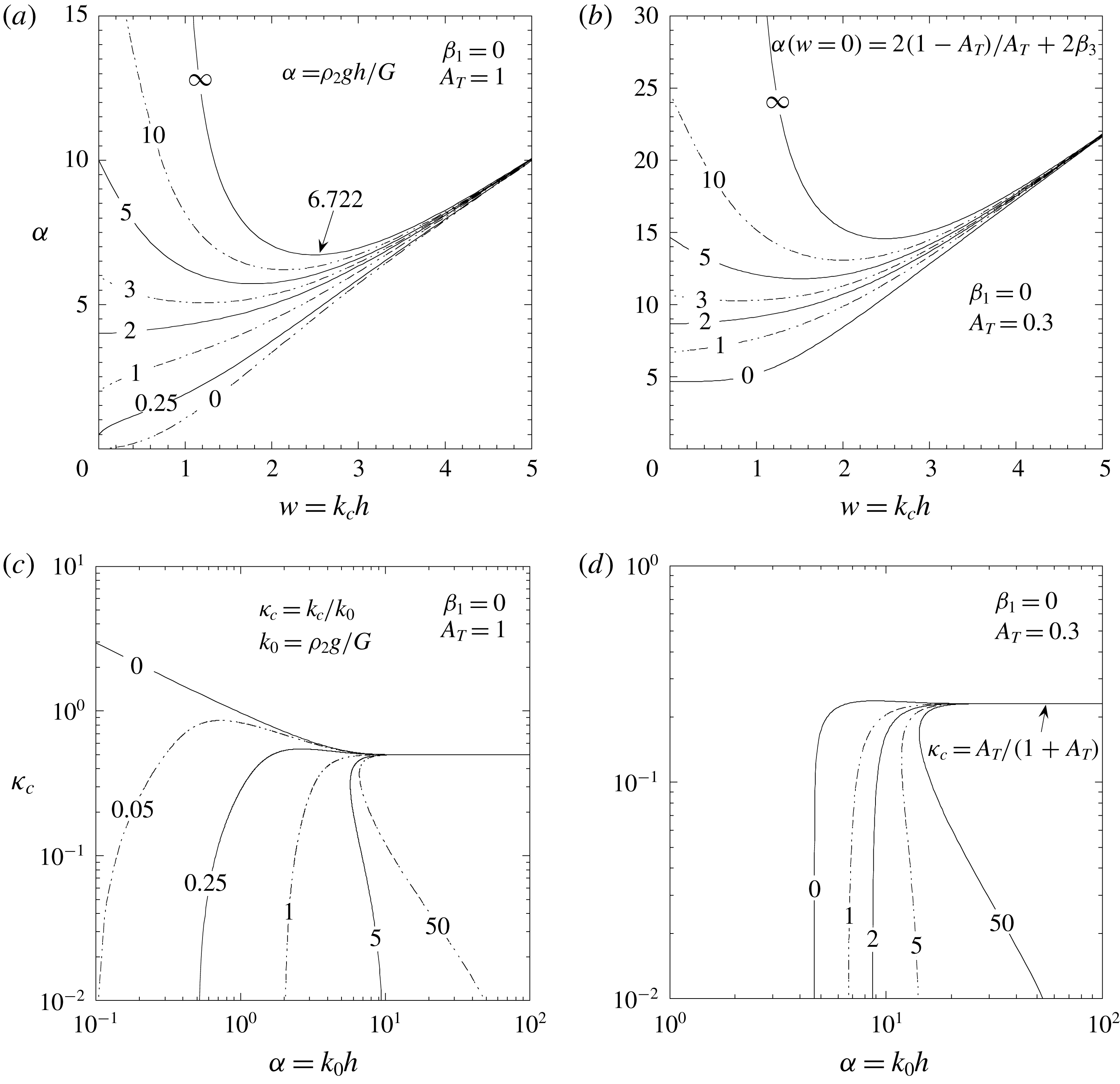
Figure 5(c,d) shows the same cases as before but for the marginal stability wavenumber
 $\unicode[STIX]{x1D705}_{c}$
as a function of dimensionless thickness
 $\unicode[STIX]{x1D6FC}$
. The behaviour is qualitatively the same for any Atwood number except for the fact that, for the purely elastic case (
 $\unicode[STIX]{x1D6FD}_{3}=0$
), there is no instability threshold when
 $A_{T}=1$
(Plohr & Sharp Reference Plohr and Sharp1998, Piriz et al.
Reference Piriz, Piriz and Tahir2017a
,Reference Piriz, Piriz and Tahir
b
).
Figure 5(a,b) also shows that there are two cut-off wavenumbers for a given value of
 $\unicode[STIX]{x1D6FC}$
when
 $\unicode[STIX]{x1D6FD}_{3}>2$
. This situation resembles the results found by Mora et al. (Reference Mora, Phou, Fromental and Pomeau2014) and Ricobelli & Ciarletta (Reference Ricobelli and Ciarletta2017) for the case of an elastic slab in contact with a rigid surface. We can analytically find the curve
 $\unicode[STIX]{x1D6FC}(w)$
for the limiting case
 $\unicode[STIX]{x1D6FD}_{3}\rightarrow \infty$
:
 $$\begin{eqnarray}\displaystyle \unicode[STIX]{x1D6FC}_{\infty }(w)={\displaystyle \frac{1+A_{T}}{2A_{T}}}{\displaystyle \frac{w(2w^{2}+2w+\sinh 2w)}{(\sinh w)^{2}-w}}. & & \displaystyle\end{eqnarray}$$
This curve has a minimum value for
 $w_{m}\approx 2.487$
, and the minimum value of
 $\unicode[STIX]{x1D6FC}_{\infty }$
is
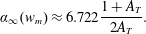 $$\begin{eqnarray}\displaystyle \unicode[STIX]{x1D6FC}_{\infty }(w_{m})\approx 6.722{\displaystyle \frac{1+A_{T}}{2A_{T}}}. & & \displaystyle\end{eqnarray}$$
The previous results are similar to the ones obtained for the case of an elastic slab with rigid wall boundary conditions. However, even for a very strong magnetic field, the case involving rigid walls is never retrieved. This is because, although the normal velocity perturbation at
 $y=-h$
,
 $\unicode[STIX]{x1D6FF}v_{2y}(-y)\rightarrow 0$
for
 $\unicode[STIX]{x1D6FD}_{3}\rightarrow \infty$
, the tangential velocity
 $\unicode[STIX]{x1D6FF}v_{2x}(-h)$
remains finite. Instead, in a rigid wall the no-slipping boundary condition imposes that
 $\unicode[STIX]{x1D6FF}v_{2x}(-h)$
must also be equal to zero. Nevertheless, the behaviour found here for
 $\unicode[STIX]{x1D6FD}_{3}>2$
may also indicate the possibility of a bifurcation leading to two different paths in the nonlinear evolution, in which the left branch of figure 5(a,b) may lead to some kind of creasing instability like the one observed by Liang & Cai (Reference Liang and Cai2015), or to some other new instability.
Besides, it is interesting to note that in this case the system stability increases with the intensity of the magnetic field
 $B_{3}$
, such as shown by (4.37) and figure 5(c,d). Such a behaviour is just the opposite to the one discussed in § 4.2.1 for
 $\unicode[STIX]{x1D6FD}_{3}=0$
and
 $\unicode[STIX]{x1D6FD}_{1}\geqslant 0$
. However, it can be qualitatively explained in the same terms as before. In fact, now the presence of the magnetic field reduces the deformation
 $\unicode[STIX]{x1D709}_{b}$
of the upper surface of the slab, and such a reduction leads to an increase of the total strain
 $(\unicode[STIX]{x1D709}_{a}-\unicode[STIX]{x1D709}_{b})/h$
for the thinner slabs. Therefore, the stabilising effect of elasticity is now reinforced by the magnetic field. In the case of a thicker slab, on the other hand, the effect of the magnetic field atop the slab is not felt and the system behaves like a purely elastic semi-infinite medium laying atop an ideal fluid.
4.2.3
$\unicode[STIX]{x1D6FD}_{1}=\unicode[STIX]{x1D6FD}_{3}\equiv \unicode[STIX]{x1D6FD}_{0}$

In this case, (4.24) and (4.25) reduce to the following expressions:
 $$\begin{eqnarray}\displaystyle & \displaystyle H_{1}(w)={\displaystyle \frac{1-A_{T}}{1+A_{T}}}\left\{{\displaystyle \frac{w[2w(1-\unicode[STIX]{x1D6FD}_{0})+\sinh 2w]}{(\sinh w)^{2}}}+2w\unicode[STIX]{x1D6FD}_{0}\right\}, & \displaystyle\end{eqnarray}$$
 $$\begin{eqnarray}\displaystyle & \displaystyle H_{2}(w)=4w^{2}\left[1-{\displaystyle \frac{(1-\unicode[STIX]{x1D6FD}_{0})^{2}w^{2}}{(\sinh w)^{2}}}\right]+4w^{2}\unicode[STIX]{x1D6FD}_{0}^{2}+4w^{2}\unicode[STIX]{x1D6FD}_{0}{\displaystyle \frac{[2w(1-\unicode[STIX]{x1D6FD}_{0})+\sinh 2w]}{(\sinh w)^{2}}}.\quad & \displaystyle\end{eqnarray}$$
For
 $w\gg 1$
these equations yield, respectively,
 $H_{1}\approx 2w(1+\unicode[STIX]{x1D6FD}_{0})$
and
 $H_{2}=[2w(1-\unicode[STIX]{x1D6FD}_{0})]^{2}$
, so we get the usual limit for thick slabs:
 $$\begin{eqnarray}\displaystyle \unicode[STIX]{x1D705}_{c}\approx {\displaystyle \frac{A_{T}}{(1+A_{T})(1+\unicode[STIX]{x1D6FD}_{0})}}. & & \displaystyle\end{eqnarray}$$
In the opposite limit
 $w\ll 1$
, we get
 $$\begin{eqnarray}\displaystyle & \displaystyle H_{1}(w)\approx 2{\displaystyle \frac{1-A_{T}}{1+A_{T}}}[2-\unicode[STIX]{x1D6FD}_{0}(1-w)], & \displaystyle\end{eqnarray}$$
 $$\begin{eqnarray}\displaystyle & \displaystyle H_{2}(w)\approx 4w^{2}\left[1-(1-\unicode[STIX]{x1D6FD}_{0})^{2}\left(1-{\displaystyle \frac{w^{2}}{3}}\right)+\unicode[STIX]{x1D6FD}_{0}^{2}\right]+8w\unicode[STIX]{x1D6FD}_{0}(2-\unicode[STIX]{x1D6FD}_{0}). & \displaystyle\end{eqnarray}$$
These limits show that (4.23) describes several different behaviours depending on the values of
 $\unicode[STIX]{x1D6FD}_{0}$
and
 $A_{T}$
which are discussed below:
(i) For
 $A_{T}=1$
and
 $\unicode[STIX]{x1D6FD}_{0}=0$
we retrieve, as expected, the pure elastic case with a cut-off given by (4.31) (Bakhrakh et al.
Reference Bakhrakh, Drennov, Kovalev, Lebedev, Meshkov, Mikhailov, Nevmerzhitsky, Nizovtsev, Rayevsky and Simonov1997, Plohr & Sharp Reference Plohr and Sharp1998, Piriz et al.
Reference Piriz, Piriz and Tahir2017a
,Reference Piriz, Piriz and Tahir
b
) (see figure 6
a, and (4.31))
Marginal stability curves for the case with equal magnetic field intensities atop and beneath the slab,
 $\unicode[STIX]{x1D6FD}_{1}=\unicode[STIX]{x1D6FD}_{3}\equiv \unicode[STIX]{x1D6FD}_{0}$
(
 $\unicode[STIX]{x1D6FD}_{n}=B_{n}^{2}/(2\unicode[STIX]{x1D707}_{n}G)$
), for two Atwood numbers (
 $A_{T}=1$
and
 $A_{T}=0.3$
), and for several values of
 $\unicode[STIX]{x1D6FD}_{0}$
(indicated by the labels on the curves). (a,b) Dimensionless cut-off wavenumber
 $\unicode[STIX]{x1D705}_{c}=w/\unicode[STIX]{x1D6FC}$
as a function of
 $\unicode[STIX]{x1D6FC}$
for
 $A_{T}=1$
and for
 $\unicode[STIX]{x1D6FD}_{0}\leqslant 1$
and
 $\unicode[STIX]{x1D6FD}_{0}\geqslant 1$
, respectively. (c) Dimensionless cut-off wavenumber
 $\unicode[STIX]{x1D705}_{c}=w/\unicode[STIX]{x1D6FC}$
as a function of
 $\unicode[STIX]{x1D6FC}$
for
 $A_{T}=0.3$
. (d) The function
 $w_{0}=w_{0}(\unicode[STIX]{x1D6FD}_{0})$
given by (4.48) for which
 $\unicode[STIX]{x1D6FC}(w_{0})=0$
.
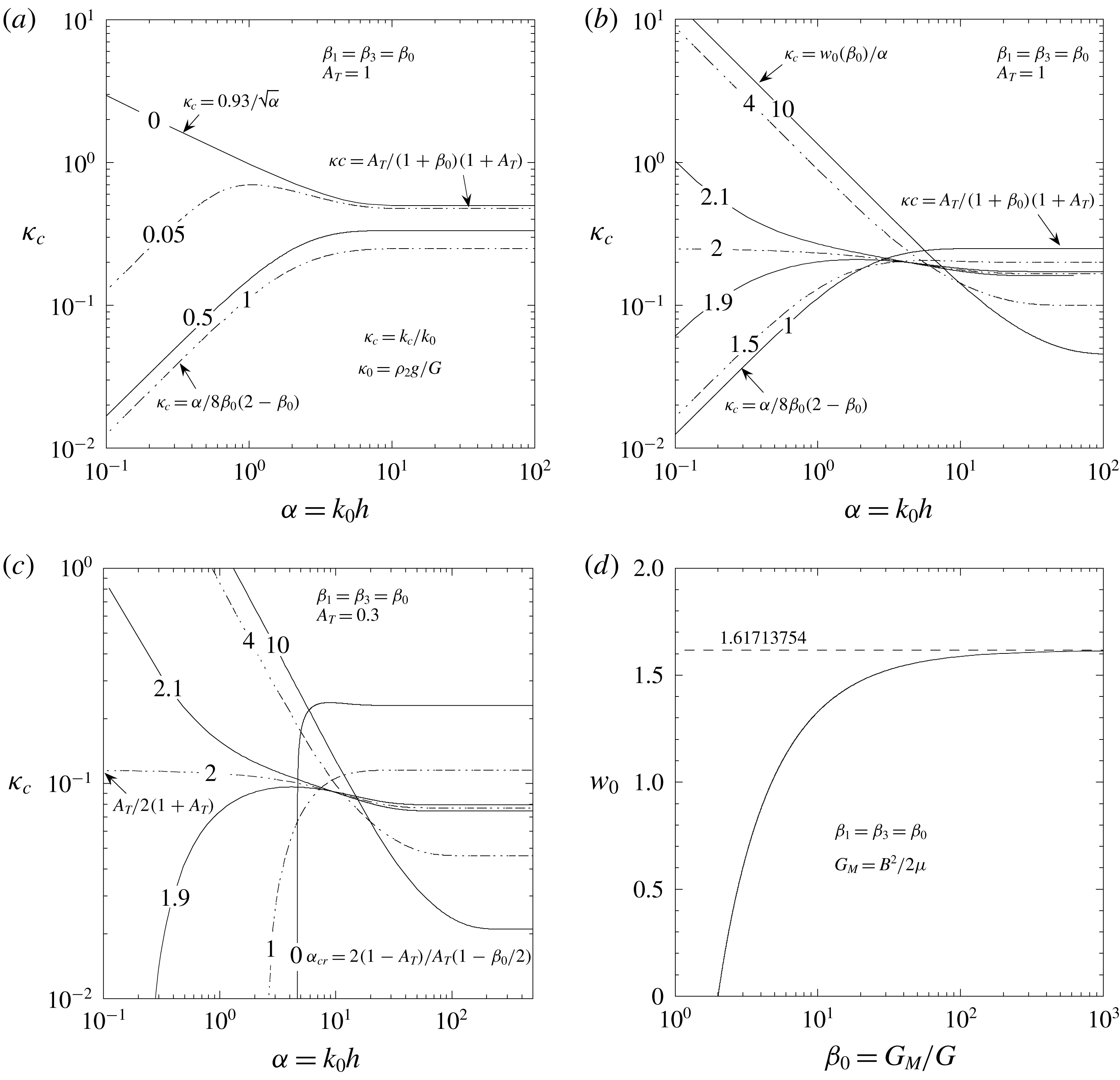
(ii) For
 $A_{T}=1$
and
 $0<\unicode[STIX]{x1D6FD}_{0}<2$
, it turns out that
 $H_{1}(w)=0$
and
 $H_{2}\approx 8w\unicode[STIX]{x1D6FD}_{0}(2-\unicode[STIX]{x1D6FD}_{0})$
, and we get
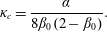 $$\begin{eqnarray}\displaystyle \unicode[STIX]{x1D705}_{c}={\displaystyle \frac{\unicode[STIX]{x1D6FC}}{8\unicode[STIX]{x1D6FD}_{0}(2-\unicode[STIX]{x1D6FD}_{0})}}. & & \displaystyle\end{eqnarray}$$
This shows that
 $\unicode[STIX]{x1D705}_{c}$
decreases as
 $\unicode[STIX]{x1D6FD}_{0}$
increases provided that
 $\unicode[STIX]{x1D6FD}_{0}\leqslant 1$
(figure 6
a). In this case, the behaviour is qualitatively similar to that observed for the case with
 $\unicode[STIX]{x1D6FD}_{1}=0$
(figure 5
a), indicating that for the smallest values of the magnetic fields the system response is dominated by the field atop the slab (for
 $\unicode[STIX]{x1D6FC}\ll 1$
).
Instead, for
 $\unicode[STIX]{x1D6FD}_{0}>1$
(figure 6
b) the behaviour is inverted and
 $\unicode[STIX]{x1D705}_{c}$
increases as the magnetic field increases (
 $\unicode[STIX]{x1D6FD}_{0}<2$
). This case, instead, is similar to that for
 $\unicode[STIX]{x1D6FD}_{3}=0$
shown in figure 2(d), indicating that as
 $\unicode[STIX]{x1D6FD}_{0}$
increases beyond
 $\unicode[STIX]{x1D6FD}_{0}>1$
the system stability becomes dominated by the magnetic field beneath the slab.
(iii) For
 $\unicode[STIX]{x1D6FD}_{0}=2$
and arbitrary
 $A_{T}$
, we have
 $H_{1}(w)\approx 2w\unicode[STIX]{x1D6FD}_{0}=4w$
and
 $H_{2}(w)\approx 4w^{2}\unicode[STIX]{x1D6FD}_{0}^{2}=(4w)^{2}$
(
 $w\ll 1$
), and the cut-off wavenumber reads (figure 6
b,c)
 $$\begin{eqnarray}\displaystyle \unicode[STIX]{x1D705}_{c}={\displaystyle \frac{A_{T}}{2(1+A_{T})}}. & & \displaystyle\end{eqnarray}$$
This value, for
 $A_{T}=1$
, is larger than the one given by (4.46) for
 $\unicode[STIX]{x1D6FD}_{0}<2$
, indicating that
 $\unicode[STIX]{x1D705}_{c}$
continues to increase with
 $\unicode[STIX]{x1D6FD}_{0}$
.
(iv) For
 $\unicode[STIX]{x1D6FD}_{0}>2$
and arbitrary
 $A_{T}$
, we can see that there exists a value
 $w_{0}$
of
 $w$
such that
 $\unicode[STIX]{x1D6FC}(w_{0})=0$
. From (4.23) we can see that this means that
 $H_{2}(w)=0$
. This condition is only satisfied for some particular values of
 $\unicode[STIX]{x1D6FD}_{0}$
, so that the function
 $w_{0}(\unicode[STIX]{x1D6FD}_{0})$
is given by the implicit function obtained by solving the equation
 $H_{2}(w_{0})=0$
:
 $$\begin{eqnarray}\displaystyle \unicode[STIX]{x1D6FD}_{0}(w_{0})={\displaystyle \frac{(w_{0}+\sinh w_{0})(1+\cosh w_{0})}{w_{0}(1+\cosh w_{0})-(\sinh w_{0})^{2}}}. & & \displaystyle\end{eqnarray}$$
Actually
 $\unicode[STIX]{x1D6FD}_{0}(w_{0})$
is more easily obtained by putting
 $C_{0}=A_{0}$
(
 $C_{1}=C_{2}\equiv C_{0}$
and
 $A_{1}=A_{2}\equiv A_{0}$
) in (4.12) and (4.13). The function
 $w_{0}(\unicode[STIX]{x1D6FD}_{0})$
has been represented in figure 6(d), and it shows that
 $w_{0}(\unicode[STIX]{x1D6FD}_{0})$
has an asymptotic value
 $w_{0\infty }\approx 1.616$
for
 $\unicode[STIX]{x1D6FD}_{0}\rightarrow \infty$
. Then, for
 $w_{0}=w_{0}(\unicode[STIX]{x1D6FD}_{0})$
one has
 $\unicode[STIX]{x1D6FC}\ll 1$
and the cut-off wavenumber reads
 $$\begin{eqnarray}\displaystyle \unicode[STIX]{x1D705}_{c}={\displaystyle \frac{w_{0}(\unicode[STIX]{x1D6FD}_{0})}{\unicode[STIX]{x1D6FC}}}, & & \displaystyle\end{eqnarray}$$
which is again larger than the value given by (4.47) for
 $\unicode[STIX]{x1D6FD}_{0}=2$
, and
 $\unicode[STIX]{x1D705}_{c}$
continues to increase with
 $\unicode[STIX]{x1D6FD}_{0}$
up to the asymptotic value
 $\unicode[STIX]{x1D705}_{c\infty }\approx 1.616/\unicode[STIX]{x1D6FC}$
.
(v) For
 $0\leqslant \unicode[STIX]{x1D6FD}_{0}\leqslant 2$
and
 $A_{T}\neq 1$
, we have, in the limit
 $w\ll 1$
,
 $H_{1}(w)\approx 2(2-\unicode[STIX]{x1D6FD}_{0})$
and
 $H_{2}(w)\approx 8\unicode[STIX]{x1D6FD}_{0}(1-\unicode[STIX]{x1D6FD}_{0})w$
. Thus, (4.23) leads to the existence of a critical value
 $\unicode[STIX]{x1D6FC}_{cr}$
for the slab instability, so that it is stable for
 $\unicode[STIX]{x1D6FC}\leqslant \unicode[STIX]{x1D6FC}_{cr}$
:
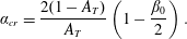 $$\begin{eqnarray}\displaystyle \unicode[STIX]{x1D6FC}_{cr}={\displaystyle \frac{2(1-A_{T})}{A_{T}}}\left(1-{\displaystyle \frac{\unicode[STIX]{x1D6FD}_{0}}{2}}\right). & & \displaystyle\end{eqnarray}$$
Similarly to the case
 $\unicode[STIX]{x1D6FD}_{3}=0$
discussed in § 4.2.1, there is an instability threshold below which the slab is stable and such a threshold progressively reduces as
 $\unicode[STIX]{x1D6FD}_{0}$
approaches the value
 $\unicode[STIX]{x1D6FD}_{0}=2$
, for which it is completely removed.
Therefore, we see that for
 $A_{T}\neq 1$
the cut-off wavenumber monotonically increases with the intensity of the magnetic fields, for the thinner slabs, in a manner similar to that which we have seen for the case
 $\unicode[STIX]{x1D6FD}_{3}=0$
. This indicates that the main conclusions obtained in such a case are still valid when
 $\unicode[STIX]{x1D6FD}_{1}\sim \unicode[STIX]{x1D6FD}_{3}$
.
4.3 Instability growth rate
We can obtain the instability growth rate
 $\unicode[STIX]{x1D6FE}$
from (4.12) to (4.19) as a function of the perturbation wavenumber
 $k$
, in terms of the thickness
 $h$
, the density
 $\unicode[STIX]{x1D70C}_{2}$
and the shear modulus
 $G$
of the elastic slab, the density
 $\unicode[STIX]{x1D70C}_{1}$
of the light medium beneath the slab and the magnetic fields
 $B_{1}$
and
 $B_{3}$
. For this, it is more convenient to use dimensionless magnitudes defined in (3.28).
Thus, after some tedious but straightforward algebra, we get the following implicit equation for
 $\unicode[STIX]{x1D70E}(\unicode[STIX]{x1D705})$
, with the parameters
 $A_{T}$
,
 $\unicode[STIX]{x1D6FC}$
,
 $\unicode[STIX]{x1D6FD}_{1}$
and
 $\unicode[STIX]{x1D6FD}_{2}$
already defined in previous sections:
 $$\begin{eqnarray}\displaystyle & & \displaystyle \displaystyle (1-\unicode[STIX]{x1D6FD}_{1})(1-\unicode[STIX]{x1D6FD}_{2})\left\{(2\unicode[STIX]{x1D705}^{2}+\unicode[STIX]{x1D70E}^{2})^{4}+16\unicode[STIX]{x1D705}^{6}(\unicode[STIX]{x1D705}^{2}+\unicode[STIX]{x1D70E}^{2})\right.\nonumber\\ \displaystyle & & \displaystyle \displaystyle \quad -\,8\unicode[STIX]{x1D705}^{3}\sqrt{\unicode[STIX]{x1D705}^{2}+\unicode[STIX]{x1D70E}^{2}}(2\unicode[STIX]{x1D705}^{2}+\unicode[STIX]{x1D70E}^{2})^{2}\left[\coth \unicode[STIX]{x1D6FC}\unicode[STIX]{x1D705}\coth \unicode[STIX]{x1D6FC}\sqrt{\unicode[STIX]{x1D705}^{2}+\unicode[STIX]{x1D70E}^{2}}\right.\nonumber\\ \displaystyle & & \displaystyle \displaystyle \quad -\left.\left.\text{csch}\,\unicode[STIX]{x1D6FC}\unicode[STIX]{x1D705}\text{csch}\,\unicode[STIX]{x1D6FC}\sqrt{\unicode[STIX]{x1D705}^{2}+\unicode[STIX]{x1D70E}^{2}}\right]\right\}\nonumber\\ \displaystyle & & \displaystyle \displaystyle \quad +\,\unicode[STIX]{x1D6FD}_{1}\unicode[STIX]{x1D6FD}_{2}\unicode[STIX]{x1D70E}^{4}\{[(2\unicode[STIX]{x1D705}^{2}+\unicode[STIX]{x1D70E}^{2})\coth \unicode[STIX]{x1D6FC}\unicode[STIX]{x1D705}+2\unicode[STIX]{x1D705}^{2}]^{2}-[(2\unicode[STIX]{x1D705}^{2}+\unicode[STIX]{x1D70E}^{2})~\text{csch}\,\unicode[STIX]{x1D6FC}\unicode[STIX]{x1D705}]^{2}\}\nonumber\\ \displaystyle & & \displaystyle \displaystyle \quad +\,[\unicode[STIX]{x1D6FD}_{1}(1-\unicode[STIX]{x1D6FD}_{3})+\unicode[STIX]{x1D6FD}_{3}(1-\unicode[STIX]{x1D6FD}_{1})]\unicode[STIX]{x1D70E}^{2}\{{\mathcal{C}}[(2\unicode[STIX]{x1D705}^{2}+\unicode[STIX]{x1D70E}^{2})\coth \unicode[STIX]{x1D6FC}\unicode[STIX]{x1D705}+2\unicode[STIX]{x1D705}^{2}]\nonumber\\ \displaystyle & & \displaystyle \displaystyle \quad -\,{\mathcal{A}}[(2\unicode[STIX]{x1D705}^{2}+\unicode[STIX]{x1D70E}^{2})\text{csch}\,\unicode[STIX]{x1D6FC}\unicode[STIX]{x1D705}]\}\nonumber\\ \displaystyle & & \displaystyle \displaystyle \quad =\unicode[STIX]{x1D705}^{2}\unicode[STIX]{x1D70E}^{4}-{\displaystyle \frac{1-A_{T}}{1+A_{T}}}\unicode[STIX]{x1D70E}^{2}(\unicode[STIX]{x1D705}+\unicode[STIX]{x1D70E}^{2})\{\unicode[STIX]{x1D705}\unicode[STIX]{x1D70E}^{2}+(1-\unicode[STIX]{x1D6FD}_{3}){\mathcal{C}}+\unicode[STIX]{x1D6FD}_{3}\unicode[STIX]{x1D70E}^{2}[(2\unicode[STIX]{x1D705}^{2}+\unicode[STIX]{x1D70E}^{2})\coth \unicode[STIX]{x1D6FC}\unicode[STIX]{x1D705}+2\unicode[STIX]{x1D705}^{2}]\}\nonumber\\ \displaystyle & & \displaystyle \displaystyle \quad -\,\unicode[STIX]{x1D705}\unicode[STIX]{x1D70E}^{2}(\unicode[STIX]{x1D6FD}_{3}-\unicode[STIX]{x1D6FD}_{1})\{{\mathcal{C}}-\unicode[STIX]{x1D70E}^{2}[(2\unicode[STIX]{x1D705}^{2}+\unicode[STIX]{x1D70E}^{2})\coth \unicode[STIX]{x1D6FC}\unicode[STIX]{x1D705}+2\unicode[STIX]{x1D705}^{2}]\},\end{eqnarray}$$
where
 $$\begin{eqnarray}\displaystyle & \displaystyle {\mathcal{A}}=(2\unicode[STIX]{x1D705}^{2}+\unicode[STIX]{x1D70E}^{2})^{2}~\text{csch}~\unicode[STIX]{x1D6FC}\unicode[STIX]{x1D705}-4\unicode[STIX]{x1D705}^{3}\sqrt{\unicode[STIX]{x1D705}^{2}+\unicode[STIX]{x1D70E}^{2}}~\text{csch}~\unicode[STIX]{x1D6FC}\sqrt{\unicode[STIX]{x1D705}^{2}+\unicode[STIX]{x1D70E}^{2}}, & \displaystyle\end{eqnarray}$$
 $$\begin{eqnarray}\displaystyle & \displaystyle {\mathcal{C}}=(2\unicode[STIX]{x1D705}^{2}+\unicode[STIX]{x1D70E}^{2})^{2}\coth \unicode[STIX]{x1D6FC}\unicode[STIX]{x1D705}-4\unicode[STIX]{x1D705}^{3}\sqrt{\unicode[STIX]{x1D705}^{2}+\unicode[STIX]{x1D70E}^{2}}\coth \unicode[STIX]{x1D6FC}\sqrt{\unicode[STIX]{x1D705}^{2}+\unicode[STIX]{x1D70E}^{2}}. & \displaystyle\end{eqnarray}$$
Expression (4.51) is a bi-quartic transcendental equation that can be shown to have a unique real and positive root for any values of the arguments when the slab is unstable. Besides, it can be shown that
 $\unicode[STIX]{x1D70E}^{2}$
is always a real number, so that solutions with oscillating perturbation growth (over-stability) do not exist (see appendix A). On the other hand, this means that for the unstable cases (
 $k<k_{c}$
) there is a growing exponential mode of the form
 $\text{e}^{+|\unicode[STIX]{x1D6FE}|t}$
and a decaying mode of the form
 $\text{e}^{-|\unicode[STIX]{x1D6FE}|t}$
, which together determine the evolution of the initial transient phase of growth for given initial conditions. Therefore, the dominant mode
 $|\unicode[STIX]{x1D70E}|$
given by (4.51) is sufficient to characterise all the possible solutions.
For obtaining (4.51) from (4.19) we have done the algebra by hand and have verified it using the Mathematica software for symbolic calculations (Wolfram Research, Inc. 2015). The same procedure has been used in the previous long algebraic manipulations.
We have represented
 $\unicode[STIX]{x1D70E}(\unicode[STIX]{x1D705})$
for two different Atwood numbers (
 $A_{T}=1$
and
 $A_{T}=0.3$
), and for the three cases considered in §§ 4.2.1–4.2.3.
Dimensionless growth rate
 $\unicode[STIX]{x1D70E}=\unicode[STIX]{x1D6FE}/\sqrt{k_{0}g}$
as a function of the dimensionless wavenumber
 $\unicode[STIX]{x1D705}=k/k_{0}$
, for the case with no magnetic field atop the slab (
 $\unicode[STIX]{x1D6FD}_{3}=0$
), for two Atwood numbers
 $A_{T}$
, and for different values of the dimensionless magnetic pressure
 $\unicode[STIX]{x1D6FD}_{1}$
(indicated by the labels on the curves) and of the dimensionless slab thickness
 $\unicode[STIX]{x1D6FC}$
: (a)
 $A_{T}=1$
and
 $\unicode[STIX]{x1D6FC}=1$
; (b)
 $A_{T}=1$
and
 $\unicode[STIX]{x1D6FC}=10$
; (c)
 $A_{T}=0.3$
and
 $\unicode[STIX]{x1D6FC}=1$
; (d)
 $A_{T}=0.3$
and
 $\unicode[STIX]{x1D6FC}=10$
.
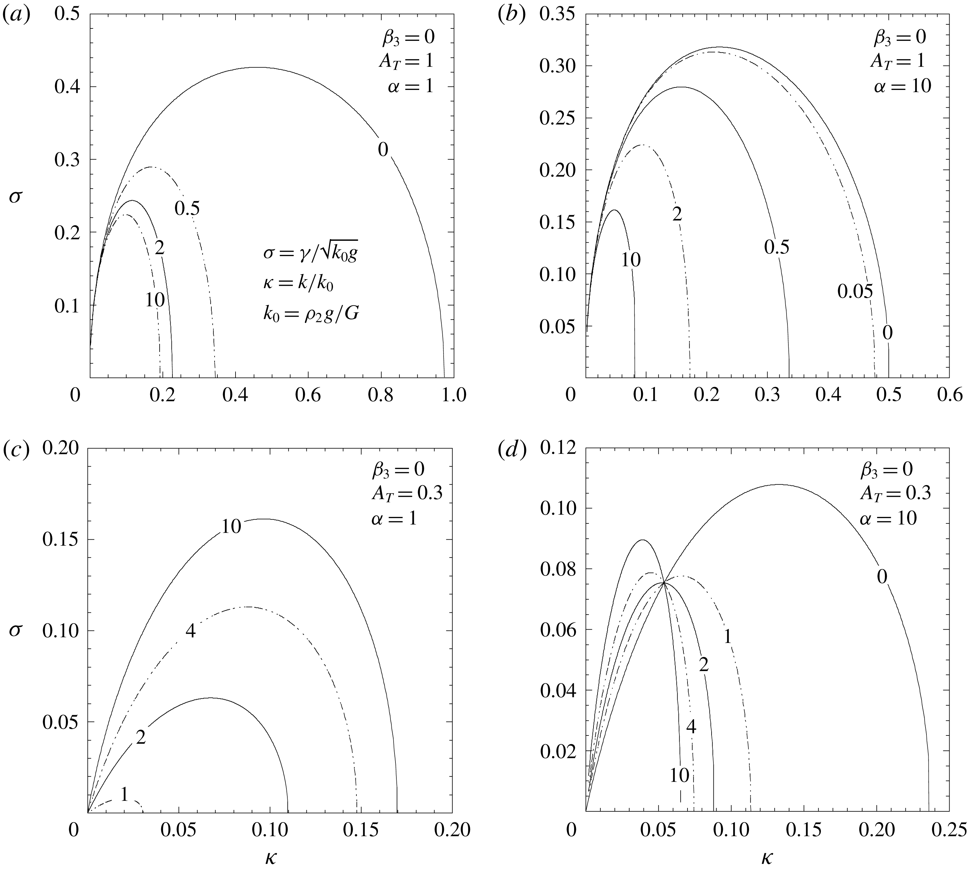
Dimensionless growth rate
 $\unicode[STIX]{x1D70E}=\unicode[STIX]{x1D6FE}/\sqrt{k_{0}g}$
as a function of the dimensionless wavenumber
 $\unicode[STIX]{x1D705}=k/k_{0}$
, for the case with no magnetic field beneath the slab (
 $\unicode[STIX]{x1D6FD}_{1}=0$
), for two Atwood numbers
 $A_{T}$
, and for different values of the dimensionless magnetic pressure
 $\unicode[STIX]{x1D6FD}_{3}$
(indicated by the labels on the curves) and of the dimensionless slab thickness
 $\unicode[STIX]{x1D6FC}$
: (a)
 $A_{T}=1$
and
 $\unicode[STIX]{x1D6FC}=1$
; (b)
 $A_{T}=1$
and
 $\unicode[STIX]{x1D6FC}=10$
; (c)
 $A_{T}=0.3$
and
 $\unicode[STIX]{x1D6FC}=10$
; (d)
 $A_{T}=0.3$
and
 $\unicode[STIX]{x1D6FC}=14$
.
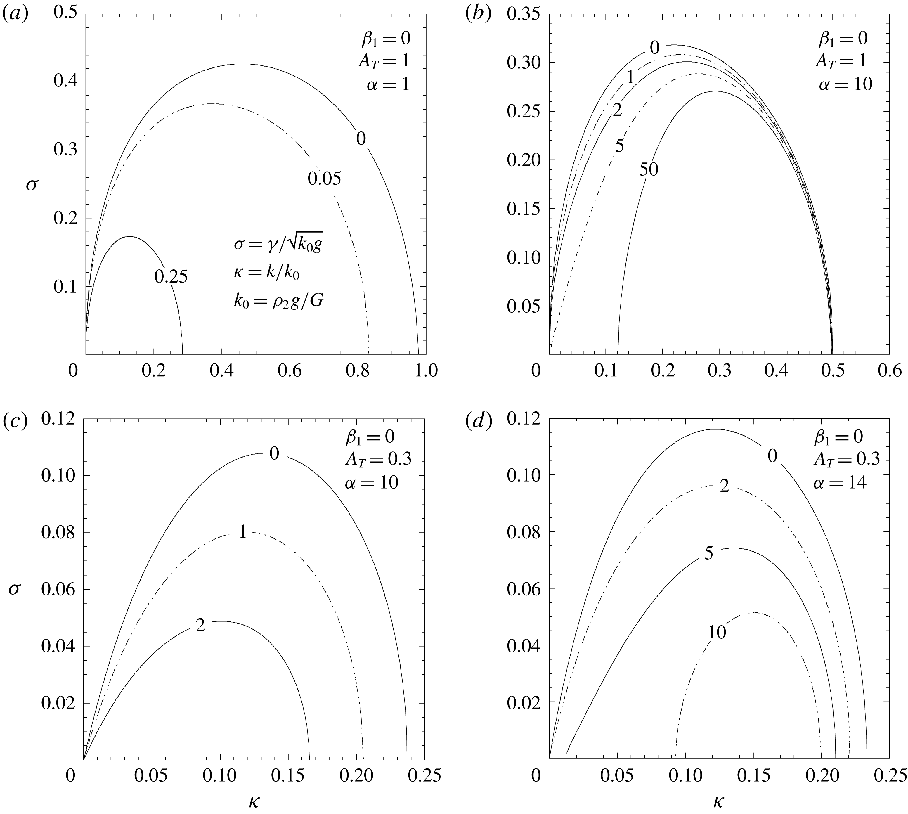
Dimensionless growth rate
 $\unicode[STIX]{x1D70E}=\unicode[STIX]{x1D6FE}/\sqrt{k_{0}g}$
as a function of the dimensionless wavenumber
 $\unicode[STIX]{x1D705}=k/k_{0}$
, for the case with equal magnetic field intensities atop and beneath the slab,
 $\unicode[STIX]{x1D6FD}_{1}=\unicode[STIX]{x1D6FD}_{3}\equiv \unicode[STIX]{x1D6FD}_{0}$
, for two Atwood numbers
 $A_{T}$
, and for different values of the dimensionless magnetic pressure
 $\unicode[STIX]{x1D6FD}_{0}$
(indicated by the labels on the curves) and of the dimensionless slab thickness
 $\unicode[STIX]{x1D6FC}$
: (a)
 $A_{T}=1$
and
 $\unicode[STIX]{x1D6FC}=1$
; (b)
 $A_{T}=1$
and
 $\unicode[STIX]{x1D6FC}=10$
; (c)
 $A_{T}=0.3$
and
 $\unicode[STIX]{x1D6FC}=1$
; (d)
 $A_{T}=0.3$
and
 $\unicode[STIX]{x1D6FC}=8$
; (e)
 $A_{T}=0.3$
and
 $\unicode[STIX]{x1D6FC}=20$
.
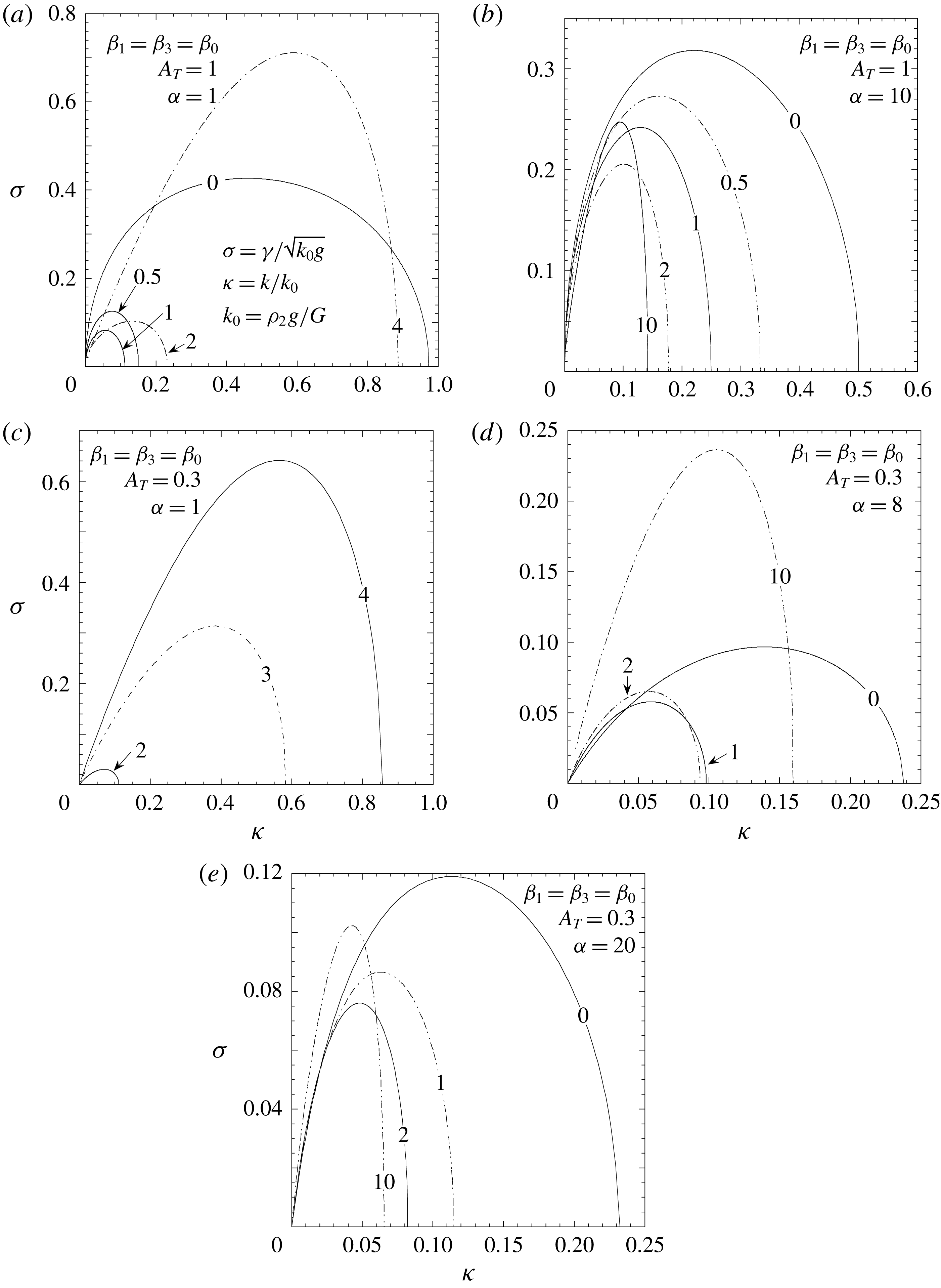
4.3.1
$\unicode[STIX]{x1D6FD}_{1}\geqslant 0$
,
$\unicode[STIX]{x1D6FD}_{3}=0$


Figures 7(a) and 7(b) show the instability growth rate for
 $A_{T}=1$
and for
 $\unicode[STIX]{x1D6FC}=1$
and
 $\unicode[STIX]{x1D6FC}=10$
, respectively, and different values of
 $\unicode[STIX]{x1D6FD}_{1}$
indicated by the labels on the curves. These two values of
 $\unicode[STIX]{x1D6FC}$
are representative of the two situations for thin and relatively thick slabs. By following the same tendency as the cut-off wavenumber, the maximum growth rate always decreases as the value of
 $\unicode[STIX]{x1D6FD}_{1}$
increases. But the growth rate reduction is less sensitive to the increase of
 $\unicode[STIX]{x1D6FD}_{1}$
for
 $\unicode[STIX]{x1D6FC}=1$
, especially for the largest values. We note that for
 $\unicode[STIX]{x1D6FC}=10$
the asymptotic regime corresponding to a semi-infinite elastic medium has not yet been reached (see figure 4
c), which is why the growth rate is somewhat higher than the one that would be obtained from (3.24).
For
 $A_{T}=0.3$
, on the other hand, the behaviour is quite different for the thin and the thick slabs, such as we have already seen in figure 4(d). In fact, figure 7(c) shows that for
 $\unicode[STIX]{x1D6FC}=1$
the growth rate monotonically decreases with
 $\unicode[STIX]{x1D6FD}_{1}$
, and it becomes
 $\unicode[STIX]{x1D6FE}=0$
for
 $\unicode[STIX]{x1D6FD}_{1}\leqslant 2(1-A_{T})/(1+A_{T})$
. For
 $\unicode[STIX]{x1D6FC}=10$
the growth rate does not decrease monotonically when
 $\unicode[STIX]{x1D6FD}_{1}$
increases as the cut-off wavenumber does (figure 7
d), but it considerably decreases for
 $0\leqslant \unicode[STIX]{x1D6FD}_{1}\leqslant 1$
and then it remains more or less the same with some increase for the largest values of
 $\unicode[STIX]{x1D6FD}_{1}$
. It is actually difficult to provide a clear physical explanation for such a behaviour since it depends on the interplay of the effects due to the presence of the lighter fluid with those of elasticity, magnetic field and slab thickness that, as we have already seen, may compete among them.
4.3.2
$\unicode[STIX]{x1D6FD}_{1}=0$
,
$\unicode[STIX]{x1D6FD}_{3}\geqslant 0$


In this case, the growth rate follows a monotonic behaviour for any value of
 $A_{T}$
and
 $\unicode[STIX]{x1D6FC}$
, in which
 $\unicode[STIX]{x1D70E}$
decreases as
 $\unicode[STIX]{x1D6FD}_{3}$
increases (figure 8). However, for
 $\unicode[STIX]{x1D6FD}_{3}>2$
(
 $\unicode[STIX]{x1D6FC}>4$
), a second cut-off appears from the side of the shortest wavenumbers that is clearly seen in figure 8(b,d) (see also figure 5
a,b). When this occurs, the classical growth rate for the RT instability (
 $\unicode[STIX]{x1D6FE}\sim \sqrt{kg}$
) usually expected for small values of the wavenumber
 $k$
is no longer retrieved.
The existence of this short-wavenumber cut-off is related to the behaviour already observed in figure 5(a,b), and, as was discussed in § 4.2.2, it is somewhat similar to what was observed by Mora et al. (Reference Mora, Phou, Fromental and Pomeau2014) and Ricobelli & Ciarletta (Reference Ricobelli and Ciarletta2017) for an elastic slab in contact with a rigid wall. But, as we have already seen, although the effect of the magnetic field above the slab is to reduce the vertical deformation of the slab top surface, it does not affect the tangential velocity. Therefore, rigid wall conditions are never retrieved even for
 $\unicode[STIX]{x1D6FD}_{3}\rightarrow \infty$
.
On the other hand, the reduction of the deformation
 $\unicode[STIX]{x1D709}_{b}$
of the top surface leads to an enhancement of the total relative deformation of the slab
 $(\unicode[STIX]{x1D709}_{a}-\unicode[STIX]{x1D709}_{b})/h$
thereby reinforcing the stabilising elasticity effectiveness. However, such an effect cannot be felt for the shortest perturbation wavelengths (
 $kh\gtrsim 1$
), which cannot ‘see’ the slab top surface and whereby the total relative deformation is instead
 $k\unicode[STIX]{x1D709}_{a}$
. As a result, the stabilising effect of the magnetic field occupying the region
 $y\leqslant -h$
is only felt for perturbation wavenumbers such that
 $kh\lesssim 1$
, which leads to a short-wavenumber cut-off.
4.3.3
$\unicode[STIX]{x1D6FD}_{1}=\unicode[STIX]{x1D6FD}_{3}\equiv \unicode[STIX]{x1D6FD}_{0}$

As is seen in § 4.2.3, this case presents some mixed characteristics of the two previous cases discussed above. In figures 9(a) and 9(b) we show the growth rate for
 $A_{T}=1$
and
 $\unicode[STIX]{x1D6FC}=1$
and
 $\unicode[STIX]{x1D6FC}=10$
, respectively. As in the previous cases, we also consider several values of
 $\unicode[STIX]{x1D6FD}_{0}$
indicated by the labels on the curves. The maximum growth rate follows the same tendency as the cut-off, namely it decreases as
 $\unicode[STIX]{x1D6FD}_{0}$
increases, provided that
 $\unicode[STIX]{x1D6FD}_{0}<1$
, while inverting this behaviour in the opposite case (see (4.46)). For
 $\unicode[STIX]{x1D6FC}=10$
,
 $\unicode[STIX]{x1D70E}$
again follows the behaviour of
 $\unicode[STIX]{x1D705}_{c}$
(figure 6
a,b) for relatively weak magnetic fields and it decreases as
 $\unicode[STIX]{x1D6FD}_{0}$
increases. But for the largest values of
 $\unicode[STIX]{x1D6FD}_{0}$
, the growth rate starts to increase. It is not completely clear what the physical reason is for this loss of stability for the most intense magnetic fields occurring in the regime of intermediate wavenumbers, and it is difficult to determine the details of the interplay among the different effects. But it seems that for the largest values of
 $\unicode[STIX]{x1D6FD}_{0}$
the magnetic field beneath the slab becomes more relevant for determining the slab stability.
For
 $A_{T}=0.3$
, we have already seen in § 4.2.3 that the cut-off wavenumber always increases with
 $\unicode[STIX]{x1D6FD}_{0}$
provided that the slab is sufficiently thin. And, according to (4.50), it becomes zero for a given value of
 $\unicode[STIX]{x1D6FC}$
when
 $\unicode[STIX]{x1D6FD}_{0}\leqslant [2-\unicode[STIX]{x1D6FC}A_{T}/(1-A_{T})]$
. Figure 9(c) shows that for
 $\unicode[STIX]{x1D6FC}=1$
, the growth rate follows the same tendency as the cut-off. But in figure 9(d) we see that the behaviour is the contrary for very large values of
 $\unicode[STIX]{x1D6FC}$
, approaching the case of two semi-infinite media.
However, for the intermediate values of
 $\unicode[STIX]{x1D6FC}$
, the interplay among the different mechanisms makes the growth rate exhibit a variety of behaviours surely depending of the relative dominance of each one of them (figure 9
d,e). As we have already discussed, we can only provide physical interpretations for the extreme cases for which some specific mechanism is seen to be dominant over the others.
5 Concluding remarks
We have presented a linear theory for the two-dimensional MRT instability in a system that is composed of an elastic layer that lies above a lighter ideal fluid. Moreover, a uniform magnetic field is present above and below this system, as shown in figure 1. Consideration of a finite thickness of the elastic layer in this work leads to the discovery of interesting new aspects of this problem, which have not been detected in previous studies that involved semi-infinite media, and/or do not consider Hookean constitutive properties of the slab.
The magnetic field which exists in the region occupied by the lighter fluid could be expected, on the basis of the results for semi-infinite media, to provide a positive and supporting contribution to the stabilising effect produced by the elasticity (addition of the two effects). However, contrary to this expectation, the magnetic field opposes the elasticity stabilisation effect when the layer is sufficiently thin. This is because, for relatively thin layers, the total strain that controls the elasticity effects is determined by the deformation of both slab interfaces, whereas the magnetic field affects mainly the face on which it is acting (see discussion in § 4.2.1). As a consequence, the influence of the magnetic field acting below the elastic layer becomes detrimental to the stabilising effects due to the elasticity which reduces the system stability. Furthermore, the instability threshold imposed by the layer elasticity is progressively reduced and even vanishes for a sufficiently large magnetic pressure (
 ${\sim}G$
).
This situation is very common in many high-energy-density physics experiments and inertial fusion schemes in which a finite-thickness slab is accelerated, or a cylindrical shell target is imploded by a magnetic pressure. The slab is maintained in a solid state with the aim of enhancing the hydrodynamic stability during acceleration. The new results that we report may be an important issue in such experiments.
In nature, the present problem is also very relevant to the triggering of crust-quakes in strongly magnetised neutron stars known as megnetars. The mechanism proposed by Blaes et al. (Reference Blaes, Blandford, Madau and Koonin1990, Reference Blaes, Blandford, Madau and Yan1992) requires a minimum inversion density in the crust in order to overtake the threshold imposed by the elasticity. It has been shown that such an inversion density can occur as a consequence of the pycnonuclear and electron capture reactions forced by the accretion of matter of neutron stars from the interstellar medium. Nevertheless, it seems quite improbable that it may have enough magnitude to exceed the instability threshold established by the crust elasticity. However, the presence of strong magnetic fields generating magnetic pressures of the order of the shear modulus
 $G$
can eliminate such a threshold and make the crust unstable for any arbitrary small density inversion. Therefore, MRT instability can be an effective process to trigger crust-quakes in magnetars when magnetic pressures of the order of the shear modulus,
 $G$
, of the crust are developed.
In a similar manner, the magnetic field on top of the elastic layer acts in support of the stabilising effects generated by elasticity, but its action on the system is limited to relatively long perturbation wavelengths (
 $kh\gtrsim 1$
). As a consequence, a short-wavenumber cut-off may exist, below which the system remains stable. This case exhibits some similarities to the RT instability in elastic layers in contact with rigid walls. This is because such a magnetic field restricts the velocity perturbation normal to the interface, while the tangential velocity is not affected and therefore the rigid wall boundary conditions are never reproduced. Nevertheless, we can speculate on the possibility that in the nonlinear regime the system may evolve towards two different instabilities (creasing and wrinkle instabilities) corresponding to each branch of short and long wavenumbers, as reported by Liang & Cai (Reference Liang and Cai2015) for the case of elastic soft materials.
On the other hand, when magnetic fields on both sides of the elastic slab are comparable, the resulting picture is a combination of the previous two extreme cases. In general, for the shortest perturbation wavelengths, the effects of the magnetic field beneath the slab become dominant, and the effects of the field atop it are felt for the thinner slabs or the longest perturbation wavelengths.
Finally, it may be worth remarking that the present linear theory assumes that the deviation from flatness of the slab is always sufficiently small, so that
 $k\unicode[STIX]{x1D709}_{a,b}\ll 1$
must be the case.
Acknowledgements
This work has been partially supported by Ministerio de Economía y Competitividad (grant no. ENE2016-75703-R), Junta de Comunidades de Castilla-La Mancha of Spain (grant no. SBPLY/17/180501/000264) and the BMBF of Germany.
Appendix A. Proof that
$\unicode[STIX]{x1D70E}^{2}$
is a real number

We start with (2.24b ) and its complex conjugate:
 $$\begin{eqnarray}\displaystyle \unicode[STIX]{x1D6FE}^{2}\unicode[STIX]{x1D713}_{2}={\displaystyle \frac{G}{\unicode[STIX]{x1D70C}_{2}}}\unicode[STIX]{x1D6FB}^{2}\unicode[STIX]{x1D713}_{2},\quad (\unicode[STIX]{x1D6FE}^{2})^{\ast }\unicode[STIX]{x1D713}_{2}^{\ast }={\displaystyle \frac{G}{\unicode[STIX]{x1D70C}_{2}}}\unicode[STIX]{x1D6FB}^{2}\unicode[STIX]{x1D713}_{2}^{\ast }, & & \displaystyle\end{eqnarray}$$
where
 $(\unicode[STIX]{x1D6FE}^{2})^{\ast }$
and
 $\unicode[STIX]{x1D713}_{2}^{\ast }$
are the complex conjugates of
 $\unicode[STIX]{x1D6FE}^{2}$
and
 $\unicode[STIX]{x1D713}_{2}$
, respectively. By multiplying the first one by
 $\unicode[STIX]{x1D713}_{2}^{\ast }$
and the second one by
 $\unicode[STIX]{x1D713}_{2}$
, and subtracting, we get
 $$\begin{eqnarray}\displaystyle [\unicode[STIX]{x1D6FE}^{2}-(\unicode[STIX]{x1D6FE}^{2})^{\ast }]|\unicode[STIX]{x1D713}_{2}|^{2}={\displaystyle \frac{G}{\unicode[STIX]{x1D70C}_{2}}}[\unicode[STIX]{x1D713}_{2}^{\ast }\unicode[STIX]{x1D6FB}^{2}\unicode[STIX]{x1D713}_{2}-\unicode[STIX]{x1D713}_{2}\unicode[STIX]{x1D6FB}^{2}\unicode[STIX]{x1D713}_{2}^{\ast }]={\displaystyle \frac{G}{\unicode[STIX]{x1D70C}_{2}}}\unicode[STIX]{x1D735}\boldsymbol{\cdot }(\unicode[STIX]{x1D713}_{2}^{\ast }\unicode[STIX]{x1D735}\unicode[STIX]{x1D713}_{2}-\unicode[STIX]{x1D713}_{2}\unicode[STIX]{x1D735}\unicode[STIX]{x1D713}_{2}^{\ast }). & & \displaystyle\end{eqnarray}$$
Integrating over the two-dimensional volume
 $V=h\ell$
(
 $\ell =2\unicode[STIX]{x03C0}/k$
is the perturbation wavelength), and then using Green’s theorem to transform the volume integral into a surface integral over the surface
 $A(V)$
of such a volume, yields
 $$\begin{eqnarray}\displaystyle [\unicode[STIX]{x1D6FE}^{2}-(\unicode[STIX]{x1D6FE}^{2})^{\ast }]\int _{V}|\unicode[STIX]{x1D713}_{2}|^{2}\,\text{d}V={\displaystyle \frac{G}{\unicode[STIX]{x1D70C}_{2}}}\int _{A(V)}(\unicode[STIX]{x1D713}_{2}^{\ast }\unicode[STIX]{x1D735}\unicode[STIX]{x1D713}_{2}-\unicode[STIX]{x1D713}_{2}\unicode[STIX]{x1D735}\unicode[STIX]{x1D713}_{2}^{\ast })\boldsymbol{\cdot }\text{d}\,\boldsymbol{A}. & & \displaystyle\end{eqnarray}$$
By performing the surface integral by parts over the surface
 $A(V)$
, we have
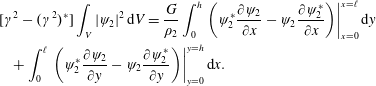 $$\begin{eqnarray}\displaystyle & & \displaystyle \displaystyle [\unicode[STIX]{x1D6FE}^{2}-(\unicode[STIX]{x1D6FE}^{2})^{\ast }]\int _{V}|\unicode[STIX]{x1D713}_{2}|^{2}\,\text{d}V={\displaystyle \frac{G}{\unicode[STIX]{x1D70C}_{2}}}\int _{0}^{h}\left.\left(\unicode[STIX]{x1D713}_{2}^{\ast }{\displaystyle \frac{\unicode[STIX]{x2202}\unicode[STIX]{x1D713}_{2}}{\unicode[STIX]{x2202}x}}-\unicode[STIX]{x1D713}_{2}{\displaystyle \frac{\unicode[STIX]{x2202}\unicode[STIX]{x1D713}_{2}^{\ast }}{\unicode[STIX]{x2202}x}}\right)\right|_{x=0}^{x=\ell }\text{d}y\nonumber\\ \displaystyle & & \displaystyle \displaystyle \quad +\int _{0}^{\ell }\left.\left(\unicode[STIX]{x1D713}_{2}^{\ast }{\displaystyle \frac{\unicode[STIX]{x2202}\unicode[STIX]{x1D713}_{2}}{\unicode[STIX]{x2202}y}}-\unicode[STIX]{x1D713}_{2}{\displaystyle \frac{\unicode[STIX]{x2202}\unicode[STIX]{x1D713}_{2}^{\ast }}{\unicode[STIX]{x2202}y}}\right)\right|_{y=0}^{y=h}\text{d}x.\end{eqnarray}$$
Since from (2.26) we have
 $$\begin{eqnarray}\displaystyle \unicode[STIX]{x1D713}_{2}=\text{e}^{\unicode[STIX]{x1D6FE}t}f(y)\cos kx,\quad \unicode[STIX]{x1D713}_{2}^{\ast }=\text{e}^{\unicode[STIX]{x1D6FE}^{\ast }t}f^{\ast }(y)\cos kx, & & \displaystyle\end{eqnarray}$$
it is straightforward to see that the integrand of the first integral is identically zero, and that the second integral is proportional to
 $\int _{0}^{\ell }\cos kx\,\text{d}x=0$
. Therefore, it turns out that
 $\unicode[STIX]{x1D6FE}^{2}=(\unicode[STIX]{x1D6FE}^{2})^{\ast }$
and
 $\unicode[STIX]{x1D70E}^{2}$
is a real number. That is, there are no oscillating growth solutions, and (4.51) gives all possible solutions for
 $\unicode[STIX]{x1D6FE}(k)$
.


 Open access

