2. Physical decomposition of mean skin friction generation in zero-pressure-gradient boundary layers

An incompressible zero-pressure-gradient smooth-flat-plate boundary layer is considered here, with free-stream velocity $U_{\infty }$ towards $x>0$ and zero instantaneous streamwise velocity at the wall ( $u(y=0)=0$ ), but free wall-normal and spanwise velocities $v(y=0)$ and $w(y=0)$ (allowing blowing/suction). The flow is assumed to be statistically stationary in time (in the reference frame of the wall) and statistically homogeneous along the spanwise direction $(z)$ . A reference frame where the wall is moving is sought so that the skin friction develops a non-zero power visible in a mean kinetic-energy budget (see the Introduction). Further, this budget should not be restricted to the conventional boundary-layer thickness, because directly taking into account the turbulent fluctuations even if they are located above $y={\it\delta}$ is one of the motivations for a decomposition different from the FIK identity (1.7). To involve all wall distances in the budget, a finite (per unit wall area) mean streamwise kinetic energy should be contained above the wall. This is the case in an absolute reference frame moving together with the undisturbed fluid at $U_{\infty }$ towards $x>0$ with respect to the wall (see figure 1). The absolute-frame coordinates $x_{A},y_{A},t_{A}$ and velocities $u_{A},v_{A}$ are related to the coordinates $x,y,t$ and velocities $u,v$ in the usual frame (attached to the wall) by the following equations:

(2.1a−e ) $$\begin{eqnarray}x_{A}=x-U_{\infty }t,\quad y_{A}=y,\quad t_{A}=t,\quad u_{A}=u-U_{\infty },\quad v_{A}=v.\end{eqnarray}$$

In the absolute frame, the wall is moving at $-U_{\infty }$ along $x_{A}$ and the undisturbed fluid outside the boundary layer has no streamwise velocity ( $u_{A}=0$ ). Since $U_{\infty }$ is constant, the absolute frame is inertial and pressure coincides in both frames ( $p_{A}=p$ ).

Figure 1.

Sketch of mean streamwise kinetic energy ( $K_{A}$ ) in an absolute reference frame.

Assuming the boundary-layer hypothesis and the validity of the boundary-layer equations (also with a possible wall blowing/suction), the mean streamwise momentum equation in the usual frame reads:

(2.2) $$\begin{eqnarray}\frac{\overline{\text{D}}\langle u\rangle }{\overline{\text{D}}t}=\frac{\partial }{\partial y}\left({\it\nu}\frac{\partial \langle u\rangle }{\partial y}-\langle u^{\prime }v^{\prime }\rangle \right),\end{eqnarray}$$

where the Reynolds average $\langle \cdot \rangle$ , seen as an ensemble average, coincides in both frames, and $\cdot ^{\prime }$ is the fluctuation. The mean material derivative, if applied to mean quantities, is $\overline{\text{D}}/\overline{\text{D}}t=\langle u\rangle \partial /\partial x+\langle v\rangle \partial /\partial y$ , as the mean flow is steady in the usual frame. The mean material derivative coincides in both frames, by definition and because time is not affected by the frame transformation ( $t_{A}=t$ ). When applied to mean quantities, it can be written as:

(2.3) $$\begin{eqnarray}\frac{\overline{\text{D}}}{\overline{\text{D}}t}=\langle u\rangle \frac{\partial }{\partial x}+\langle v\rangle \frac{\partial }{\partial y}=\frac{\partial }{\partial t_{A}}+\langle u_{A}\rangle \frac{\partial }{\partial x_{A}}+\langle v_{A}\rangle \frac{\partial }{\partial y_{A}},\end{eqnarray}$$

where it is emphasized that the mean flow is unsteady in the absolute frame because of its streamwise heterogeneity.

In the absolute frame, the momentum equation (2.2) becomes:

(2.4) $$\begin{eqnarray}\frac{\overline{\text{D}}\langle u_{A}\rangle }{\overline{\text{D}}t}=\frac{\partial }{\partial y_{A}}\left({\it\nu}\frac{\partial \langle u_{A}\rangle }{\partial y_{A}}-\langle u_{A}^{\prime }v_{A}^{\prime }\rangle \right)=\frac{\partial }{\partial y_{A}}\left(\frac{{\it\tau}}{{\it\rho}}\right),\end{eqnarray}$$

where the total shear stress is ${\it\tau}/{\it\rho}={\it\nu}(\partial \langle u\rangle /\partial y)-\langle u^{\prime }v^{\prime }\rangle ={\it\nu}(\partial \langle u_{A}\rangle /\partial y_{A})-\langle u_{A}^{\prime }v_{A}^{\prime }\rangle$ . Multiplying by $\langle u_{A}\rangle$ brings the budget of the absolute-frame mean streamwise kinetic energy $K_{A}=\langle u_{A}\rangle ^{2}/2$ :

(2.5) $$\begin{eqnarray}\underbrace{\frac{\overline{\text{D}}K_{A}}{\overline{\text{D}}t}}_{\substack{ \text{variation of }K_{A} \\ \text{with boundary} \\ \text{layer growth} \\ {\hookrightarrow}C_{f,c}(2.6)}}=\underbrace{\langle u_{A}\rangle \frac{\partial }{\partial y_{A}}\left(\frac{{\it\tau}}{{\it\rho}}\right)}_{\substack{ \text{power of viscous} \\ \text{and turbulent efforts} \\ {\hookrightarrow}C_{f,c}(2.8)}}=\underbrace{\frac{\partial }{\partial y_{A}}\left(\langle u_{A}\rangle \frac{{\it\tau}}{{\it\rho}}\right)}_{\substack{ \text{viscous and turbulent} \\ \text{diffusion of }K_{A} \\ {\hookrightarrow}C_{f}(2.6),(2.8)}}\underbrace{-{\it\nu}\left(\frac{\partial \langle u_{A}\rangle }{\partial y_{A}}\right)^{2}}_{\substack{ \text{direct dissipation} \\ \text{of }K_{A} \\ {\hookrightarrow}C_{f,a}(2.6),(2.8)}}+\underbrace{\langle u_{A}^{\prime }v_{A}^{\prime }\rangle \frac{\partial \langle u_{A}\rangle }{\partial y_{A}}}_{\substack{ \text{`dissipation' of }K_{A} \\ \text{by turbulent kinetic} \\ \text{energy production} \\ {\hookrightarrow}C_{f,b}(2.6),(2.8)}},\end{eqnarray}$$

where diffusive and dissipative terms have been split. The mean streamwise kinetic-energy budget (2.5) is integrated over all $y_{A}\geqslant 0$ (using the conditions $\langle u_{A}\rangle (y_{A}=0)=-U_{\infty }$ and $u_{A}^{\prime }(y_{A}=0)=0$ implied by the assumption $u(y=0)=0$ ) and non-dimensionalised by $U_{\infty }^{3}/2$ to obtain a local (in $x_{A}$ ) decomposition of the mean skin friction coefficient $C_{f}={\it\tau}(y_{A}=0)/(1/2{\it\rho}U_{\infty }^{2})$ (1.1), involving physical phenomena occurring at all wall distances:

(2.6) $$\begin{eqnarray}C_{f}=\underbrace{\frac{2}{U_{\infty }^{3}}\int _{0}^{\infty }{\it\nu}\left(\frac{\partial \langle u_{A}\rangle }{\partial y_{A}}\right)^{2}\,\text{d}y_{A}}_{C_{f,a}}+\underbrace{\frac{2}{U_{\infty }^{3}}\int _{0}^{\infty }-\langle u_{A}^{\prime }v_{A}^{\prime }\rangle \frac{\partial \langle u_{A}\rangle }{\partial y_{A}}\,\text{d}y_{A}}_{C_{f,b}}+\underbrace{\frac{2}{U_{\infty }^{3}}\int _{0}^{\infty }\frac{\overline{\text{D}}K_{A}}{\overline{\text{D}}t}\,\text{d}y_{A}}_{C_{f,c}}.\end{eqnarray}$$

The origin of each term is emphasized in the mean streamwise kinetic energy budget (2.5). The energy transfers seen here in the absolute reference frame (attached to the undisturbed outer fluid) differ significantly from the common analysis performed in the usual reference frame (attached to the wall). $C_{f}$ represents the mean power supplied by the wall to the fluid in the absolute frame, diffusing through the boundary-layer profile with a direct (i.e. viscous) dissipation ( $C_{f,a}$ ) and with ‘dissipation’ by all the production of turbulent kinetic energy at $x_{A}$ ( $C_{f,b}$ ). The term $C_{f,b}$ does not necessarily coincide with turbulent dissipation, and it is not properly speaking a dissipation term, since turbulent kinetic energy (TKE) production is not associated with irreversible entropy creation. $C_{f,c}$ represents the rate at which absolute-frame mean streamwise kinetic energy is gained by the fluid, i.e. the part of mean skin friction power not dissipated into heat and turbulent kinetic energy. Consequently, $C_{f,c}/C_{f}$ is the efficiency of the wall supplying mean streamwise kinetic energy to the fluid in the absolute frame. $C_{f,a}$ and $C_{f,c}$ directly depend on the mean field only, whereas $C_{f,b}$ explicitly depends on the turbulent fluctuations, suggesting that $C_{f,b}$ represents the turbulence-induced excess friction (but the other terms indirectly depend on turbulence through its effect on the mean field). If integrated over $x_{A}$ , the decomposition with zero pressure gradient is consistent with the global drag decomposition mathematically derived by Drela (Reference Drela2009) with perturbation velocities in the usual (wall) frame.

Although the decomposition (2.6) has its physical interpretation rooted in the absolute reference frame, for its practical use, it is more conveniently rewritten as a function of the usual (wall) reference frame variables. Invoking (2.3) together with the definitions $K_{A}=1/2\langle u_{A}\rangle ^{2}$ and $u_{A}=u-U_{\infty }$ leads to:

(2.7) $$\begin{eqnarray}\displaystyle C_{f} & = & \displaystyle \underbrace{\frac{2}{U_{\infty }^{3}}\int _{0}^{\infty }{\it\nu}\left(\frac{\partial \langle u\rangle }{\partial y}\right)^{2}\,\text{d}y}_{C_{f,a}}+\underbrace{\frac{2}{U_{\infty }^{3}}\int _{0}^{\infty }-\langle u^{\prime }v^{\prime }\rangle \frac{\partial \langle u\rangle }{\partial y}\,\text{d}y}_{C_{f,b}}\nonumber\\ \displaystyle & & \displaystyle +\,\underbrace{\frac{2}{U_{\infty }^{3}}\int _{0}^{\infty }(\langle u\rangle -U_{\infty })\left(\langle u\rangle \frac{\partial \langle u\rangle }{\partial x}+\langle v\rangle \frac{\partial \langle u\rangle }{\partial y}\right)\,\text{d}y}_{C_{f,c}},\end{eqnarray}$$

where it clearly appears that $C_{f,c}$ represents the spatial growth of the flow, which is interpreted as the rate of gain of mean streamwise kinetic energy by the fluid in the absolute frame. However, the numerical assessment of the explicit streamwise derivative contained in $C_{f,c}$ (2.7) may cause difficulties, and the needed $x$ -dependent information is not always included in experimental or numerical datasets. Moreover, most of the established self-similarity properties describe local (in $x$ ) profiles rather than their streamwise evolution. The explicit dependence of $C_{f,c}$ on $x$ -derivatives may be avoided, using (2.5) to relate the spatial growth to the wall-normal variations of total shear stress. Equation (2.6) is finally rewritten as a function of the usual frame variables in a form that only depends on well-documented profiles at the considered streamwise station (the origin of each term is indicated in (2.5)):

(2.8) $$\begin{eqnarray}\displaystyle C_{f} & = & \displaystyle \underbrace{\frac{2}{U_{\infty }^{3}}\int _{0}^{\infty }{\it\nu}\left(\frac{\partial \langle u\rangle }{\partial y}\right)^{2}\,\text{d}y}_{C_{f,a}}+\underbrace{\frac{2}{U_{\infty }^{3}}\int _{0}^{\infty }-\langle u^{\prime }v^{\prime }\rangle \frac{\partial \langle u\rangle }{\partial y}\,\text{d}y}_{C_{f,b}}\nonumber\\ \displaystyle & & \displaystyle +\,\underbrace{\frac{2}{U_{\infty }^{3}}\int _{0}^{\infty }(\langle u\rangle -U_{\infty })\frac{\partial }{\partial y}\left(\frac{{\it\tau}}{{\it\rho}}\right)\,\text{d}y}_{C_{f,c}}.\end{eqnarray}$$

The resulting decomposition (2.8) is purely local in $x$ since the term $C_{f,c}$ (2.8) no longer explicitly involves a streamwise derivative. The spatial growth of the flow is still represented by $C_{f,c}$ (2.8), since it may also be written as in (2.7) (using (2.5) or (2.2)). Moreover, the integrands vary in the streamwise direction, and so does $C_{f}$ . Equations (2.6)–(2.8) are three ways of writing the same decomposition $C_{f}=C_{f,a}+C_{f,b}+C_{f,c}$ and may be used equivalently, as the integrands of each term locally coincide (note that this is similar to the FIK identity which has two equivalent forms (1.5) and (1.7)). The last form (2.8) will be preferred for the practical evaluation of the decomposition, while the first form (2.6) should be kept in mind when the physical interpretation of the decomposition is considered. Assuming that the TKE production term is non-negative and that the total shear stress is a non-increasing function of wall distance (so that $(U_{\infty }-\langle u\rangle )(\partial /\partial y)({\it\tau}/{\it\rho})\leqslant 0$ ), the form (2.8) involving usual flow variables may be used to conclude that the integrands of all three terms are non-negative at all $y$ , as will be seen in figures 2 and 5, so that the efficiency $C_{f,c}/C_{f}$ satisfies:

(2.9) $$\begin{eqnarray}0\leqslant C_{f,c}/C_{f}\leqslant 1.\end{eqnarray}$$

In its (2.8) form, the decomposition could be directly derived from the second equation (2.5) relating shear stresses (total, viscous and Reynolds stresses). This short route, enabling a very quick and simple derivation of the present decomposition, is established in appendix B. However, the physical interpretation requires the explicit consideration of the absolute-frame mean streamwise kinetic energy $K_{A}$ , whose budget (2.5) naturally leads to the first form (2.6) of the decomposition.

Considering the global budgets of mean streamwise kinetic energy in the usual frame (attached to the wall) $K=\langle u\rangle ^{2}/2$ , as found in textbooks such as Hinze (Reference Hinze1959), and also in the absolute frame $K_{A}=\langle u_{A}\rangle ^{2}/2$ (2.6), leads to the following relation:

(2.10) $$\begin{eqnarray}C_{f}=\underbrace{-\frac{2}{U_{\infty }^{3}}\int _{0}^{\infty }\frac{\overline{\text{D}}K}{\overline{\text{D}}t}\,\text{d}y}_{C_{f,a}+C_{f,b}}+\underbrace{\frac{2}{U_{\infty }^{3}}\int _{0}^{\infty }\frac{\overline{\text{D}}K_{A}}{\overline{\text{D}}t}\,\text{d}y}_{C_{f,c}}=\frac{2}{U_{\infty }^{3}}\int _{0}^{\infty }\frac{\overline{\text{D}}}{\overline{\text{D}}t}(K_{A}-K)\,\text{d}y,\end{eqnarray}$$

where the fact that direct dissipation and TKE production are the same in both frames has been used. This equation illustrates the importance of the choice of the reference frame. Indeed, mean skin friction does not appear in the usual-frame budget of $K$ (Hinze Reference Hinze1959) but it is present in the absolute-frame budget of $K_{A}$ (2.6).

Figure 2.

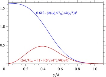
Integrands of the mean skin friction generation decomposition (2.8) rewritten in the laminar zero-pressure-gradient boundary layer (3.1) from the Blasius solution (Schlichting Reference Schlichting1968).  $0.612(\partial (\langle u\rangle /U_{\infty })/\partial (y/{\it\delta}))^{2}$ : integrand of $C_{f,a,lam}$ (blue); $(\langle u\rangle /U_{\infty }-1)(\partial /\partial (y/{\it\delta}))(({\it\tau}/{\it\rho})^{+})$ : integrand of $C_{f,c,lam}$ (red); both normalised by the total $C_{f,lam}$ .

Even though the FIK identity (1.7) and the present decomposition (2.8) share undeniable similarities, their derivations are fundamentally different. The FIK decomposition results from integrating by parts three times a momentum budget in the usual frame (appendix A), whereas the present decomposition is obtained by only one integration of a kinetic-energy budget in an absolute frame. The physical interpretation of this unique integration is straightforward, as it provides the global budget for the whole boundary-layer profile from the local (in $y_{A}$ ) budget (2.5). Moreover, splitting the diffusive and dissipative terms before integrating the local budget is equivalent to integrating $\langle u_{A}\rangle (\partial /\partial y_{A})({\it\tau}/{\it\rho})$ by parts, showing that this integration by parts mathematically represents the derivation of the present decomposition and has the clear physical meaning of distinguishing between diffusive and dissipative contributions to the global budget.

The upper bound of the integrals of the present decomposition (2.8) is not limited to $y={\it\delta}$ , contrary to the FIK identity (1.7), meaning that the turbulent fluctuations located in the whole boundary-layer profile are explicitly taken into account by $C_{f,b}$ in (2.8), whereas only the fluctuations at $y\leqslant {\it\delta}$ are present in $C_{f,II}$ (1.7). Besides, $C_{f,b}$ (2.8) represents the integral of the turbulent kinetic-energy production distribution, which may also be seen as the distribution of Reynolds shear stress weighted by the mean velocity gradient. This weight increases when the wall distance decreases, so that the closer to the wall, the larger the effect of a Reynolds-shear-stress-carrying turbulent fluctuation on mean skin friction. This conclusion was already obtained from the $C_{f,II}$ term of the FIK identity (1.7), but with a different (linear) increase of the weight function when the wall distance decreases. The mean velocity gradient weight in the present $C_{f,b}$ (2.8) has an obvious physical interpretation since the product is equal to turbulent kinetic-energy production, contrary to the linearly-weighted Reynolds shear stress involved in $C_{f,II}$ (1.7) where neither the linear weight function $(1-y/{\it\delta})$ nor the obtained distribution correspond to the profile of a physical quantity known to the authors in a zero-pressure-gradient flat-plate turbulent boundary layer.

The above discussion shows that the present decomposition (2.8) addresses some of the issues raised in the introduction related to the FIK identity (1.7). However, at first sight the difficulties to use the FIK identity in spatially-developing flows, related to the $C_{f,III}$ (1.7) term and to the indirect relation between the turbulence-induced excess friction and $C_{f,II}$ (1.7), as discussed in the introduction, may similarly be encountered with the present decomposition. The term $C_{f,c}$ (2.8), which represents the spatial growth of the boundary layer (as seen in the form (2.7)), depends on the turbulent fluctuations (even though this dependence is only implicit if $C_{f,c}$ is written in the forms (2.6) or (2.7)). Consequently, a direct and explicit link between the term $C_{f,b}$ (2.8) and the turbulence-induced excess friction cannot be established without further analysis. In the case of the FIK identity (1.7), the difficulty cannot be fully overcome because $C_{f,III}$ (1.7) does not become negligible compared with $C_{f,II}$ at high Reynolds numbers, as shown by Deck et al. (Reference Deck, Renard, Laraufie and Weiss2014). In order to better understand the relative importance of $C_{f,b}$ and $C_{f,c}$ (2.8), the Reynolds-number dependence of the present decomposition (2.8) is discussed in the following. It will then be shown how the issue related to the term $C_{f,c}$ may be addressed.

3. Reynolds-number effect on mean skin friction generation

We investigate here the Reynolds-number effect on the skin friction decomposition (2.8) in the smooth-flat-plate zero-pressure-gradient laminar and turbulent boundary layers, with no-slip velocities at the impermeable wall ( $u=v=w=0$ at $y=0$ ).

3.1. Laminar zero-pressure-gradient boundary layer

In the laminar zero-pressure-gradient case, assuming that the flow is the self-similar Blasius solution and using its numerical approximation by Schlichting (Reference Schlichting1968), (2.8) becomes:

(3.1) $$\begin{eqnarray}\displaystyle C_{f,lam} & = & \displaystyle \underbrace{C_{f,lam}\cdot \int _{0}^{\infty }0.612\left(\frac{\partial (\langle u\rangle /U_{\infty })}{\partial (y/{\it\delta})}\right)^{2}\,\text{d}(y/{\it\delta})}_{C_{f,a,lam}}\nonumber\\ \displaystyle & & \displaystyle +\,\underbrace{C_{f,lam}\cdot \int _{0}^{\infty }\left(\frac{\langle u\rangle }{U_{\infty }}-1\right)\frac{\partial }{\partial (y/{\it\delta})}\left(\left(\frac{{\it\tau}}{{\it\rho}}\right)^{+}\right)\,\text{d}(y/{\it\delta})}_{C_{f,c,lam}},\end{eqnarray}$$

where quantities non-dimensionalised by the wall values are denoted by $\bullet ^{+}$ , the expression for $C_{f,a,lam}$ is obtained using the relation $C_{f,lam}\approx 3.267/Re_{{\it\delta}}$ , leading to the factor $0.612\approx 2/3.267$ and the expression for $C_{f,c,lam}$ is obtained using the relation $C_{f,lam}=({\it\tau}/{\it\rho})(y=0)/(1/2\,U_{\infty }^{2})$ . Figure 2 shows the normalised integrands of $C_{f,a,lam}$ and $C_{f,c,lam}$ . The area below the integrand of $C_{f,a,lam}$ is proportional to the rate of heat gained by the fluid by direct dissipation in this laminar flow. The area below the integrand of $C_{f,c,lam}$ is proportional to the rate of absolute-frame mean streamwise kinetic energy gained by the fluid. The total area below both laminar integrands is proportional to the power supplied by the wall to the fluid in the absolute frame, through skin friction. The Reynolds-number invariance of the laminar integrands of (3.1), illustrated by figure 2 (which represents the profiles at any Reynolds number), implies that the ratio $C_{f,c,lam}/C_{f,lam}$ is constant. Consequently, the laminar efficiency ( $C_{f,c,lam}/C_{f,lam}\approx 0.214$ ) at which the fluid gains mean streamwise kinetic energy from the work done in the absolute reference frame by the friction force exerted by the moving wall is Reynolds-number invariant, consistent with the assumption of a self-similar flow. It is low, which is not surprising for viscous entrainment. Little kinetic energy is gained near the wall, and more in the core of the profile (see the integrand of $C_{f,c,lam}$ in figure 2). The direct dissipation of the lost fraction ( $C_{f,a,lam}/C_{f,lam}\approx 0.786$ ) is especially high near the wall, but both processes widely overlap (figure 2).

Figure 3.

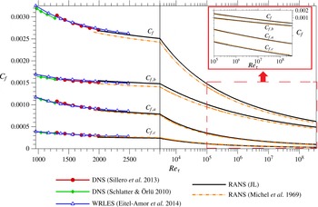
Dependence of the decomposition of $C_{f}$ (2.8) on the friction Reynolds number $Re_{{\it\tau}}$ in the turbulent zero-pressure-gradient boundary layer. DNS by Sillero, Jimenez & Moser (Reference Sillero, Jimenez and Moser2013) (see also Sillero, Jimenez & Moser Reference Sillero, Jimenez and Moser2014) and Schlatter & Örlü (Reference Schlatter and Örlü2010). Wall-resolved LES by Eitel-Amor, Örlü & Schlatter (Reference Eitel-Amor, Örlü and Schlatter2014). RANS simulations with Jones & Launder (Reference Jones and Launder1972)  $k$ – ${\it\epsilon}$ (JL) model and Michel, Quémard & Durant (Reference Michel, Quémard and Durant1969) model. $C_{f}$ plotted in logarithmic scale in the inset.

3.2. Turbulent zero-pressure-gradient boundary layer

The impact of the friction Reynolds number ( $Re_{{\it\tau}}={\it\delta}u_{{\it\tau}}/{\it\nu}$ , ${\it\tau}/{\it\rho}\,(y=0)=u_{{\it\tau}}^{2}$ ) on the decomposition (2.8) is assessed in the turbulent case in figure 3. Direct numerical simulation (DNS) and wall-resolved large-eddy simulation datasets are used together with high-Reynolds-number Reynolds-averaged Navier–Stokes (RANS) simulations from the ONERA boundary-layer code CLICET (Aupoix Reference Aupoix2010). This code has been used in studies such as Aupoix & Spalart (Reference Aupoix and Spalart2003) and the grid convergence is checked. Two very different RANS modelling strategies are considered, the Jones & Launder (Reference Jones and Launder1972) $k$ – ${\it\epsilon}$ (JL) model and the Michel et al. (Reference Michel, Quémard and Durant1969) mixing-length model further described in Cousteix (Reference Cousteix1989).

Figure 3 shows that the efficiency $C_{f,c}/C_{f}$ is smaller than in the laminar case (it is even smaller than $0.15$ at all the Reynolds numbers shown in this figure). The production term $C_{f,b}$ has the slowest decay and gets close to $C_{f}$ at very high Reynolds numbers, as may be seen in the inset where $C_{f}$ is plotted in logarithmic scale.

Figure 4.

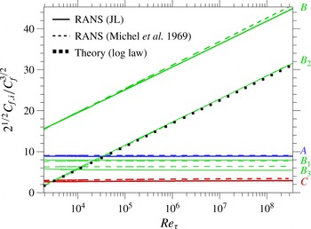
Dependence on the friction Reynolds number $Re_{{\it\tau}}$ of the functions $A(Re_{{\it\tau}})$ (blue), $B(Re_{{\it\tau}})$ (green) and $C(Re_{{\it\tau}})$ (red) defined in the form (3.2) of (2.8), and of the zonal functions $B_{1}(Re_{{\it\tau}})$ , $B_{2}(Re_{{\it\tau}})$ , $B_{3}(Re_{{\it\tau}})$ defined in (3.3), as predicted by the RANS simulations with the Jones & Launder (Reference Jones and Launder1972)  $k$ – ${\it\epsilon}$ (JL) model and the Michel et al. (Reference Michel, Quémard and Durant1969) model. The theoretical prediction shown for $B_{2}(Re_{{\it\tau}})$ represents (3.4).

The integrands of (2.8) are non-dimensionalised according to high-Reynolds-number self-similarity in the inner layer (in wall units) and in the outer layer (commonly assumed universal profiles $(U_{\infty }-\langle u\rangle )/u_{{\it\tau}}(y/{\it\delta})$ and ${\it\tau}^{+}(y/{\it\delta})$ at high Reynolds numbers, George (Reference George2006)), using the relations $\sqrt{C_{f}/2}=u_{{\it\tau}}/U_{\infty }$ and ${\it\tau}/{\it\rho}\,(y=0)=u_{{\it\tau}}^{2}$ :

(3.2) $$\begin{eqnarray}\displaystyle C_{f}=C_{f}\sqrt{\frac{C_{f}}{2}} & & \displaystyle \left(\underbrace{\int _{0}^{\infty }\left(\frac{\partial \langle u\rangle ^{+}}{\partial y^{+}}\right)^{2}\,\text{d}y^{+}}_{A(Re_{{\it\tau}})}+\underbrace{\int _{0}^{\infty }-\langle u^{\prime }v^{\prime }\rangle ^{+}\frac{\partial \langle u\rangle ^{+}}{\partial y^{+}}\,\text{d}y^{+}}_{B(Re_{{\it\tau}})}\right.\nonumber\\ \displaystyle & & \displaystyle \left.+\underbrace{\int _{0}^{\infty }\frac{\langle u\rangle -U_{\infty }}{u_{{\it\tau}}}\frac{\partial }{\partial (y/{\it\delta})}\left(\left(\frac{{\it\tau}}{{\it\rho}}\right)^{+}\right)\,\text{d}(y/{\it\delta})}_{C(Re_{{\it\tau}})}\right).\end{eqnarray}$$

Direct dissipation (represented by $C_{f,a}$ in (2.8), i.e. $C_{f}\sqrt{C_{f}/2}\,A(Re_{{\it\tau}})$ in (3.2)) occurs mostly in the inner layer where most of the mean gradients are concentrated, as will be seen in figure 5. The inner-layer universal wall law $\langle u\rangle ^{+}(y^{+})$ implies that 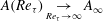$A(Re_{{\it\tau}})\underset{Re_{{\it\tau}}\rightarrow \infty }{\rightarrow }A_{\infty }$ , as will be illustrated by figure 4. As for $C_{f,c}$ (i.e. $C_{f}\sqrt{C_{f}/2}\,C(Re_{{\it\tau}})$ in (3.2)), the total shear stress significantly varies only in the outer layer, where the assumed universal laws $(U_{\infty }-\langle u\rangle )/u_{{\it\tau}}(y/{\it\delta})$ and ${\it\tau}^{+}(y/{\it\delta})$ imply that 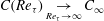$C(Re_{{\it\tau}})\underset{Re_{{\it\tau}}\rightarrow \infty }{\rightarrow }C_{\infty }$ (figure 4).

Figure 5.

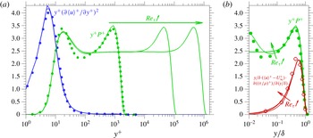
Premultiplied integrands of the friction generation decomposition (2.8) non-dimensionalised in (3.2), in the zero-pressure-gradient turbulent boundary layer. $y^{+}(\partial \langle u\rangle ^{+}/\partial y^{+})^{2}$ : premultiplied integrand of $C_{f,a}$ (blue); $y^{+}P^{+}=-y^{+}\langle u^{\prime }v^{\prime }\rangle ^{+}(\partial \langle u\rangle ^{+}/\partial y^{+})=-y/{\it\delta}\,\langle u^{\prime }v^{\prime }\rangle ^{+}(\partial \langle u\rangle ^{+}/\partial (y/{\it\delta}))$ : premultiplied integrand of $C_{f,b}$ (green); $(y/{\it\delta})((\langle u\rangle -U_{\infty })/u_{{\it\tau}})(\partial /\partial (y/{\it\delta}))(({\it\tau}/{\it\rho})^{+})$ : premultiplied integrand of $C_{f,c}$ (red); all three integrands normalised by $C_{f}\sqrt{C_{f}/2}$ . Symbols: DNS by Sillero et al. (Reference Sillero, Jimenez and Moser2013) at $Re_{{\it\theta}}=6500$ ( $Re_{{\it\tau}}=1989$ ). Lines: RANS simulations at $Re_{{\it\tau}}=2000$ , $Re_{{\it\tau}}=10^{5}$ and $Re_{{\it\tau}}=10^{6}$ (Michel et al. (Reference Michel, Quémard and Durant1969) model).

Concerning $C_{f,b}$ (i.e. $C_{f}\sqrt{C_{f}/2}\,B(Re_{{\it\tau}})$ in (3.2)), since turbulent kinetic-energy production is significantly present in both the inner and outer layers, this term is split into three zones separated by $y^{+}=100$ and $y/{\it\delta}=0.1$ :

(3.3) $$\begin{eqnarray}\displaystyle B(Re_{{\it\tau}}) & = & \displaystyle \underbrace{\int _{0}^{100}-\langle u^{\prime }v^{\prime }\rangle ^{+}\frac{\partial \langle u\rangle ^{+}}{\partial y^{+}}\,\text{d}y^{+}}_{B_{1}(Re_{{\it\tau}})}+\underbrace{\int _{100}^{0.1Re_{{\it\tau}}}-\langle u^{\prime }v^{\prime }\rangle ^{+}\frac{\partial \langle u\rangle ^{+}}{\partial y^{+}}\,\text{d}y^{+}}_{B_{2}(Re_{{\it\tau}})}\nonumber\\ \displaystyle & & \displaystyle +\,\underbrace{\int _{0.1}^{\infty }-\langle u^{\prime }v^{\prime }\rangle ^{+}\frac{\partial \langle u\rangle ^{+}}{\partial (y/{\it\delta})}\,\text{d}(y/{\it\delta})}_{B_{3}(Re_{{\it\tau}})}.\end{eqnarray}$$

The assumed inner-layer universal law implies that $B_{1}(Re_{{\it\tau}})\underset{Re_{{\it\tau}}\rightarrow \infty }{\rightarrow }B_{1\infty }$ whereas the assumed outer-layer universal laws imply that $B_{3}(Re_{{\it\tau}})\underset{Re_{{\it\tau}}\rightarrow \infty }{\rightarrow }B_{3\infty }$ . As for the layer $100\leqslant y^{+}\leqslant 0.1Re_{{\it\tau}}$ , assuming that a logarithmic velocity profile $\partial \langle u\rangle ^{+}/\partial y^{+}=1/({\it\kappa}y^{+})$ exists at least in this region together with an approximately constant Reynolds shear stress $-\langle u^{\prime }v^{\prime }\rangle ^{+}\approx 1$ leads to $B_{2}(Re_{{\it\tau}})\approx 1/{\it\kappa}(\ln (0.1Re_{{\it\tau}})-\ln (100))$ , that is:

(3.4) $$\begin{eqnarray}B_{2}(Re_{{\it\tau}})\approx \frac{1}{{\it\kappa}}\ln (Re_{{\it\tau}})+B_{2\infty }\quad (B_{2\infty }=-\!16.8~\text{for}~{\it\kappa}=0.41).\end{eqnarray}$$

The theoretical trends predicted for the functions $A(Re_{{\it\tau}})$ , $B(Re_{{\it\tau}})$ , $B_{1}(Re_{{\it\tau}})$ , $B_{2}(Re_{{\it\tau}})$ , $B_{3}(Re_{{\it\tau}})$ and $C(Re_{{\it\tau}})$ defined in (3.2) and (3.3) are in excellent agreement with both RANS models, as illustrated by figure 4. This is not a surprising result, because the construction of the RANS models involves the same assumptions as some of the assumptions used here to analyse (3.2). However, different assumptions could be used for the study of (2.8), such as the existence of a power law rather than of a logarithmic law, because these assumptions are not needed to derive the decomposition (2.8) and have been invoked only when discussing the theoretical high-Reynolds-number trends of the decomposition. If a RANS model based on a power-law assumption was used, one may expect the results to be in agreement with a theoretical analysis of the trends of (2.8) based on a power-law assumption. This has however not been tested here because of the wide agreement on the existence of a logarithmic law in flat-plate boundary layers, and because RANS models are usually based on the logarithmic-law assumption, not on a power law.

The asymptotic trends of (3.2) predicted by theory and illustrated in figure 4 suggest that $C_{f,a}$ , $C_{f,b,1}$ (part of $C_{f,b}$ corresponding to $0\leqslant y^{+}\leqslant 100$ ), $C_{f,b,3}$ (part of $C_{f,b}$ corresponding to $y/{\it\delta}\geqslant 0.1$ ) and $C_{f,c}$ behave proportionally to $C_{f}^{3/2}$ for $Re_{{\it\tau}}\rightarrow \infty$ , while the dominant term $C_{f,b,2}$ behaves as $C_{f}$ , consistent with figure 3. $C_{f,c}/C_{f}$ vanishes for $Re_{{\it\tau}}\rightarrow \infty$ , contrary to the constant laminar efficiency. The almost invariant $B_{1}$ in figure 4 represents turbulent kinetic energy production in the buffer layer, which is the zone of largest contribution to $C_{f,b}$ at low Reynolds numbers, consistent with Orlandi & Jiménez (Reference Orlandi and Jiménez1994), but is dominated by the logarithmic layer ( $B_{2}$ ) at high Reynolds numbers, whose increasing relative contribution to turbulent kinetic-energy production has been emphasized by Marusic et al. (Reference Marusic, Mathis and Hutchins2010) (see further discussions by Smits et al. (Reference Smits, McKeon and Marusic2011) and Jiménez (Reference Jiménez2013)).

The wall-normal decomposition of skin friction (2.8) is detailed in figure 5 with the non-dimensionalisation adopted in (3.2). The area below the premultiplied integrands of the normalised $C_{f,a}$ , $C_{f,b}$ and $C_{f,c}$ in semi-logarithmic scale is proportional to the contribution to $C_{f}$ . These areas represent the rate of heat gained by the fluid because of the strain rate of mean velocity, the rate of turbulent kinetic energy gained by the fluid by production and the rate of absolute-frame mean streamwise kinetic energy $K_{A}$ gained by the fluid, respectively. The total area below all three integrands represents the mean power supplied by the wall to the fluid through skin friction in the absolute frame. Some of it is dissipated by viscous mean gradients (rate of heat gained by the fluid because of the strain rate of mean velocity) mostly near the wall. It is also dissipated by turbulent kinetic-energy production in the buffer layer and in the logarithmic layer (rate of turbulent kinetic energy gained by the fluid) during its diffusion in near-constant total shear-stress layers towards the wake region. In the wake region, further dissipation occurs (mainly into turbulent kinetic energy). The remaining mean streamwise kinetic energy $K_{A}$ is gained by the fluid at a non-zero rate wherever the total shear stress varies, i.e. in particular in the wake region. Figure 5 illustrates the inner and outer-layer self-similarity (quasi-invariance of normalised integrands with respect to the Reynolds number). Contrasting with the overlapping areas of significant direct dissipation and rate of gain of $K_{A}$ in the laminar case (figure 2), in the turbulent case there is a widening separation, when the Reynolds number increases, between direct dissipation, occurring mostly near the wall, and the rate of gain of $K_{A}$ , a significant part of which occurs in the wake region. In between, the inner-scaled width of the logarithmic layer increases with $Re_{{\it\tau}}$ and results in the evolution of $B_{2}(Re_{{\it\tau}})$ shown in figure 4. The logarithmic layer may be seen as a widening intermediate zone where the rate of gain of $K_{A}$ is small (because the total shear stress is nearly constant) while $K_{A}$ is dissipated during its diffusion towards the wake region, where the rate of gain of $K_{A}$ is significant. This emphasizes the role of the logarithmic layer in the vanishing efficiency $C_{f,c}/C_{f}\underset{Re_{{\it\tau}}\rightarrow \infty }{\rightarrow }0$ at which $K_{A}$ is supplied to the fluid by the wall in the turbulent case, unlike its finite constant value in the laminar boundary layer.

4. On the relation between the generation of the turbulence-induced excess friction and turbulent kinetic-energy production in the logarithmic layer

Dividing (3.2) by $C_{f}\sqrt{C_{f}/2}$ and using the relation $\sqrt{C_{f}/2}=u_{{\it\tau}}/U_{\infty }$ , the asymptotic trends obtained in § 3.2 lead to:

(4.1) $$\begin{eqnarray}\sqrt{\frac{2}{C_{f}}}=U_{\infty }^{+}\underset{Re_{{\it\tau}}\rightarrow \infty }{=}A_{\infty }+B_{1\infty }+\frac{1}{{\it\kappa}}\ln (Re_{{\it\tau}})+B_{2\infty }+B_{3\infty }+C_{\infty }+o(1)\end{eqnarray}$$

consistent with the Coles–Fernholz correlation for skin friction and with the logarithmic/wake outer law $\langle u\rangle ^{+}=1/{\it\kappa}\ln (y^{+})+\mathscr{B}+({\it\Pi}/{\it\kappa})W(y/{\it\delta})$ assessed at $y={\it\delta}$ (Nagib, Chauhan & Monkewitz (Reference Nagib, Chauhan and Monkewitz2007), where ${\it\delta}$ is specifically defined from the wake law, only here, and such that $\langle u\rangle (y={\it\delta})=U_{\infty }$ , excluding definitions such as the 99 % thickness that may be considered in the rest of the paper).

The fact that a logarithmic friction law is obtained again illustrates the consistency of the decomposition (2.8) with assumptions made to analyse its integrands (e.g. logarithmic law). Any assumption can be made in the analysis of the decomposition (2.8), because no such assumption has been made to obtain (2.8). Moreover, the straightforward physical interpretation of the decomposition explains the close relation between the assumption (logarithmic growth of the inner-scaled turbulent kinetic-energy production contained within the logarithmic layer) and the resulting logarithmic friction law. On the contrary, it does not seem possible to the authors to predict a logarithmic friction law by inserting the assumption of the existence of a logarithmic layer into the FIK decomposition (1.7), especially because $C_{f,II}$ (1.7) does not explicitly involve the mean velocity profile.

Equation (4.1) is dominated by the behaviour of the production of turbulent kinetic energy in the logarithmic layer represented by $B_{2}(Re_{{\it\tau}})\underset{Re_{{\it\tau}}\rightarrow \infty }{=}1/{\it\kappa}\ln (Re_{{\it\tau}})+B_{2\infty }+o(1)$ , leading to $C_{f}/2\underset{Re_{{\it\tau}}\rightarrow \infty }{{\sim}}({\it\kappa}/\ln (Re_{{\it\tau}}))^{2}$ , showing together with (3.2) and (3.3) that $C_{f,a}/C_{f}$ , $C_{f,b,1}/C_{f}$ , $C_{f,b,3}/C_{f}$ and $C_{f,c}/C_{f}$ vanish when $Re_{{\it\tau}}\rightarrow \infty$ whereas $C_{f}\underset{Re_{{\it\tau}}\rightarrow \infty }{{\sim}}C_{f,b}\underset{Re_{{\it\tau}}\rightarrow \infty }{{\sim}}C_{f,b,2}$ .

As mentioned in the introduction, the turbulence-induced excess friction may be seen as the difference between the mean skin friction coefficient in the turbulent and in the laminar cases at the same Reynolds number $Re_{def}$ (1.2). The turbulent and laminar boundary layers may be compared at the same $Re_{{\it\tau}}$ (chosen as $Re_{def}$ ). The friction coefficient in the laminar case is given by $C_{f,lam}=5.34/Re_{{\it\tau}}^{2}$ , as estimated from Schlichting (Reference Schlichting1968). From the previous conclusions (especially $C_{f,turb}/2\underset{Re_{{\it\tau}}\rightarrow \infty }{{\sim}}({\it\kappa}/\ln (Re_{{\it\tau}}))^{2}$ ), the turbulence-induced excess friction $\mathscr{E}\{C_{f}(Re_{{\it\tau}})\}$ (1.2) becomes:

(4.2) $$\begin{eqnarray}\mathscr{E}\{C_{f}(Re_{{\it\tau}})\}\underset{Re_{{\it\tau}}\rightarrow \infty }{{\sim}}C_{f,turb}(Re_{{\it\tau}})\underset{Re_{{\it\tau}}\rightarrow \infty }{{\sim}}C_{f,b}(Re_{{\it\tau}})\underset{Re_{{\it\tau}}\rightarrow \infty }{{\sim}}C_{f,b,2}(Re_{{\it\tau}}).\end{eqnarray}$$

This suggests that $\mathscr{E}\{C_{f}(Re_{{\it\tau}})\}$ is directly equivalent at very high Reynolds numbers to $C_{f,b,2}$ , representing turbulent kinetic-energy production in the logarithmic layer. Consequently, the relation between $\mathscr{E}\{C_{f}\}$ and $C_{f,b}$ (2.8) is direct. On the contrary, the largest term of the FIK decomposition (1.7), $C_{f,II}$ , approximately amounts to only 80 % of $\mathscr{E}\{C_{f}\}$ (Deck et al. Reference Deck, Renard, Laraufie and Weiss2014), so that the relation between $\mathscr{E}\{C_{f}\}$ and $C_{f,II}$ is only indirect and involves $C_{f,III}$ (1.7). Since the behaviour of $C_{f,a}$ , $C_{f,b,1}$ , $C_{f,b,3}$ and $C_{f,c}$ (2.8) is approximately proportional to $C_{f}^{3/2}$ (see § 3.2), their contribution to $\mathscr{E}\{C_{f}\}$ becomes much smaller than the contribution from $C_{f,b,2}$ at very high Reynolds numbers. However, each of these terms is itself much larger than the laminar skin friction $C_{f,lam}$ at the same high value of $Re_{{\it\tau}}$ .

From an applicative point of view, the turbulence-induced excess friction should rather be considered by comparing the turbulent and laminar cases at the same Reynolds number $Re_{x}$ based on the streamwise distance from the (possibly virtual) origin. The laminar coefficient $C_{f,lam}=0.664/\sqrt{Re_{x}}$ decreases with $Re_{x}$ much faster than the turbulent coefficient $C_{f,turb}$ (one can show that $C_{f,turb}/2\underset{Re_{x}\rightarrow \infty }{{\sim}}({\it\kappa}/\ln (Re_{x}))^{2}$ , consistent with Monkewitz, Chauhan & Nagib (Reference Monkewitz, Chauhan and Nagib2007), by applying results of Nagib et al. (Reference Nagib, Chauhan and Monkewitz2007) to the $C_{f}(Re_{{\it\tau}})$ law (4.1)). Since $C_{f,turb}(Re_{x})$ dominates $C_{f,lam}(Re_{x})$ , one may conclude that $\mathscr{E}\{C_{f}(Re_{x})\}$ (1.2) is equivalent to:

(4.3) $$\begin{eqnarray}\mathscr{E}\{C_{f}(Re_{x})\}\underset{Re_{x}\rightarrow \infty }{{\sim}}C_{f,turb}(Re_{x})\underset{Re_{x}\rightarrow \infty }{{\sim}}C_{f,b}(Re_{x})\underset{Re_{x}\rightarrow \infty }{{\sim}}C_{f,b,2}(Re_{x})\end{eqnarray}$$

showing again that the turbulence-induced excess friction at very high Reynolds numbers is associated with turbulent kinetic-energy production in the logarithmic layer. However, for the same reasons as with the $Re_{def}=Re_{{\it\tau}}$ reasoning, the other terms $C_{f,a}(Re_{x})$ , $C_{f,b,1}(Re_{x})$ , $C_{f,b,3}(Re_{x})$ and $C_{f,c}(Re_{x})$ , even though negligible compared with $C_{f,b,2}(Re_{x})$ , dominate $C_{f,lam}(Re_{x})$ at the same $Re_{x}$ when $Re_{x}\rightarrow \infty$ . This suggests the relevance of seeking a Reynolds-number definition other than $Re_{{\it\tau}}$ or $Re_{x}$ to compare the laminar and turbulent values of $C_{f}$ .

The turbulent and laminar cases may be considered at the same Reynolds number $Re_{{\it\delta}_{a}}=(U_{\infty }{\it\delta}_{a})/{\it\nu}$ based on the direct dissipation thickness ${\it\delta}_{a}=1/(\int _{0}^{\infty }(\partial (\langle u\rangle /U_{\infty })/\partial y)^{2}\,\text{d}y)$ defined by Hinze (Reference Hinze1959). Having the same $Re_{{\it\delta}_{a}}$ is equivalent to having the same $C_{f,a}=2/Re_{{\it\delta}_{a}}$ by definition of ${\it\delta}_{a}$ and of $C_{f,a}$ (2.8). Moreover, the ratio $C_{f,c}/C_{f,a}$ is constant in the laminar boundary layer, $C_{f,c,lam}/C_{f,a,lam}=0.27$ , as may be seen from the results of § 3.1. In the turbulent case, figure 4 suggests that this ratio has a finite high-Reynolds-number limit $C_{f,c,turb}/C_{f,a,turb}\underset{Re_{{\it\tau}}\rightarrow \infty }{\rightarrow }C_{\infty }/A_{\infty }\approx 0.35$ . Consequently, in a laminar or in a turbulent boundary layer at the same very high $Re_{{\it\delta}_{a}}$ , $C_{f,a}$ (2.8) is the same by definition, and $C_{f,c}$ (2.8) is of the same order of magnitude, because the constants 0.27 and 0.35 are of the same order of magnitude. The turbulent $C_{f,a}$ and $C_{f,c}$ are dominated by $C_{f,b}$ (2.8) and are comparable to $C_{f,a,lam}$ and to $C_{f,c,lam}$ at the same $Re_{{\it\delta}_{a}}$ . Consequently, $\mathscr{E}\{C_{f}(Re_{{\it\delta}_{a}})\}$ is close to $C_{f,b,turb}(Re_{{\it\delta}_{a}})$ , and the difference between them ( $\mathscr{E}\{C_{f}(Re_{{\it\delta}_{a}})\}-C_{f,b,turb}(Re_{{\it\delta}_{a}})$ ) does not dominate $C_{f,lam}(Re_{{\it\delta}_{a}})$ , contrary to the comparisons for $Re_{def}=Re_{{\it\tau}}$ or $Re_{x}$ . The comparison of the laminar and turbulent cases with the Reynolds-number definition $Re_{def}=Re_{{\it\delta}_{a}}$ suggests that the essential physical cause of the turbulence-induced excess friction is the total turbulent kinetic-energy production represented by $C_{f,b}$ (2.8), which is itself equivalent at high Reynolds numbers to the turbulent kinetic-energy production within the logarithmic layer, represented by $C_{f,b,2}$ (the difference $(C_{f,b,turb}(Re_{{\it\delta}_{a}})-C_{f,b,2,turb}(Re_{{\it\delta}_{a}}))$ does not dominate $C_{f,lam}(Re_{{\it\delta}_{a}})$ either).

The established direct relation between $C_{f,b}$ (2.8) and $\mathscr{E}\{C_{f}\}$ addresses the issue identified in the introduction regarding the indirect relation between $C_{f,II}$ and $\mathscr{E}\{C_{f}\}$ by the FIK decomposition (1.7). The term $C_{f,III}$ of the FIK identity (1.7) is non-zero in spatially-developing flows and does not become negligible compared with $C_{f,II}$ at high Reynolds numbers (see Deck et al. Reference Deck, Renard, Laraufie and Weiss2014). In the present decomposition (2.8) on the contrary, $C_{f,b}$ dominates at high Reynolds numbers the other terms of the decomposition, including the non-zero $C_{f,c}$ term associated with spatial growth.

The dominant role played by the logarithmic-layer dynamics in mean skin friction generation predicted by the present decomposition (2.8) is consistent with the general importance of the logarithmic layer in high Reynolds-number wall-bounded turbulence studied and reviewed by Marusic et al. (Reference Marusic, Mathis and Hutchins2010), Smits et al. (Reference Smits, McKeon and Marusic2011) and Jiménez (Reference Jiménez2013) among others. The present study quantifies for the first time the role of the logarithmic layer in the specific question of mean skin friction. The conclusions agree with the literature on high-Reynolds-number boundary layers, which focused on quantities such as total turbulent kinetic energy production or total turbulent dissipation, not on mean skin friction.

It should be noted that a very different conclusion is obtained from the FIK decomposition (1.7). The relative contribution of the logarithmic layer to the turbulence-induced excess friction at high Reynolds numbers may be assessed according to the FIK identity by decomposing $C_{f,II}$ (1.7). Indeed, Deck et al. (Reference Deck, Renard, Laraufie and Weiss2014) showed that the turbulence-induced excess friction at high Reynolds number is approximately equal to $1.25\;C_{f,II}$ . This is a consequence of the ratio $(C_{f,I}+C_{f,II})/C_{f}$ being close to 0.8 in both the laminar and the high-Reynolds-number turbulent cases, as discussed by Deck et al. (Reference Deck, Renard, Laraufie and Weiss2014), leading to $\mathscr{E}\{C_{f}(Re_{{\it\alpha}})\}=C_{f,turb}(Re_{{\it\alpha}})-C_{f,lam}(Re_{{\it\alpha}})\approx \mathscr{G}\cdot C_{f,II}(Re_{{\it\alpha}})$ with $\mathscr{G}\approx 1/0.8=1.25$ as already mentioned in the introduction. The turbulence-induced excess friction may consequently be related to $C_{f,II}$ only, in an indirect manner. The contribution $C_{f,II,2}$ of the zone $100\leqslant y^{+}\leqslant 0.1Re_{{\it\tau}}$ to $C_{f,II}$ (1.7) is defined as follows:

(4.4) $$\begin{eqnarray}C_{f,II,2}=4\int _{100/Re_{{\it\tau}}}^{0.1}\frac{\langle -u^{\prime }v^{\prime }\rangle }{U_{\infty }^{2}}\left(1-\frac{y}{{\it\delta}}\right)\,\text{d}\left(\frac{y}{{\it\delta}}\right).\end{eqnarray}$$

At high Reynolds numbers, assuming an almost constant Reynolds shear stress $-\langle u^{\prime }v^{\prime }\rangle \approx u_{{\it\tau}}^{2}$ within this zone, one may write, using the relation $C_{f}/2=u_{{\it\tau}}^{2}/U_{\infty }^{2}$ :

(4.5) $$\begin{eqnarray}C_{f,II,2}\underset{Re_{{\it\tau}}\rightarrow \infty }{{\approx}}4\int _{0}^{0.1}\frac{u_{{\it\tau}}^{2}}{U_{\infty }^{2}}\left(1-\frac{y}{{\it\delta}}\right)\,\text{d}\left(\frac{y}{{\it\delta}}\right)=0.19\,C_{f}.\end{eqnarray}$$

Besides, since $C_{f,I}$ is negligible compared with $C_{f,II}$ in the high-Reynolds-number turbulent boundary layer, the ratio $C_{f,II}/C_{f}$ is very close to $(C_{f,I}+C_{f,II})/C_{f}$ , itself close to 0.8. From this result and (4.5), one concludes that the ratio $C_{f,II,2}/C_{f,II}$ is close to $0.19/0.8$ at high Reynolds numbers. The zone $100\leqslant y^{+}\leqslant 0.1Re_{{\it\tau}}$ , whose lower and upper bounds coincide with values typically accepted to define the logarithmic-layer range, consequently contributes only approximately 24 % of $C_{f,II}$ (1.7) at high Reynolds numbers. Thus the FIK identity predicts that the logarithmic layer is responsible for only one quarter of the turbulence-induced excess friction at asymptotically high Reynolds numbers. The remaining three quarters are mostly contributed by the wake region (this is clearly suggested by figure 16 of Deck et al. (Reference Deck, Renard, Laraufie and Weiss2014), with the premultiplied integrand of $C_{f,II}$ (1.7), $y/{\it\delta}\cdot F_{R}=4\,y/{\it\delta}\,(\langle -u^{\prime }v^{\prime }\rangle /U_{\infty }^{2})(1-y/{\it\delta})$ , plotted in semi-logarithmic scales so that the relative contribution to $C_{f,II}$ is proportional to the area below the curve). The very different wall-normal distributions of the contributions to the turbulence-induced excess friction obtained using the FIK identity (1.7) and the present decomposition (2.8) are related to the significant difference between the linearly-weighted Reynolds shear-stress profile constituting the integrand of $C_{f,II}$ in the FIK relation (1.7) and the turbulent kinetic-energy production profile which is the integrand of $C_{f,b}$ in the present decomposition (2.8). The prediction from the FIK decomposition (1.7) that the logarithmic layer would contribute only one quarter of the turbulence-induced excess friction at high Reynolds numbers is not consistent with the well-established dominant role of the logarithmic-layer dynamics at high Reynolds numbers, contrary to the results obtained with the present decomposition (2.8). The straightforward physical interpretation of the present relation (2.8) and the explicit representation of the spatial distribution of the physical phenomena by the integral of the quantities locally representing these phenomena is probably the key to the consistency between the predictions obtained and the known physical properties of high-Reynolds-number boundary layers. These advantages show the interest of the present decomposition as a complementary approach to the FIK identity.

In the presence of an inner-scaled very-near-wall flow control, a new inner law should arise, while the outer universal laws should not be modified. Considering which results of the discussion in § 3.2 are related to the inner law and which are related to the outer laws suggests that only $A_{\infty }$ and $B_{1\infty }$ are affected in (4.1), and become $A_{\infty }+{\rm\Delta}A_{\infty }$ and $B_{1\infty }+{\rm\Delta}B_{1\infty }$ . Because the control is assumed to be inner scaled, ${\rm\Delta}A_{\infty }$ and ${\rm\Delta}B_{1\infty }$ are Reynolds-number invariant. At the same $Re_{{\it\tau}}$ , $U_{\infty }^{+}$ becomes $U_{\infty }^{+}+{\rm\Delta}U^{+}$ , where ${\rm\Delta}U^{+}={\rm\Delta}A_{\infty }+{\rm\Delta}B_{1\infty }$ is Reynolds-number invariant, a prediction from the present decomposition coinciding with the observed behaviour of inner-scaled roughness or riblets (Jiménez Reference Jiménez2004; García-Mayoral & Jiménez Reference García-Mayoral and Jiménez2011; Spalart & McLean Reference Spalart and McLean2011; Aupoix, Pailhas & Houdeville Reference Aupoix, Pailhas and Houdeville2012; Bannier, Garnier & Sagaut Reference Bannier, Garnier and Sagaut2015). Note that strictly speaking, the present decomposition (2.8) does not apply to a non-smooth wall, but it is compatible with blowing/suction. The predicted behaviour results in the decay of the relative friction reduction, as ${\rm\Delta}U^{+}/U_{\infty }^{+}$ decreases with the Reynolds number, a very well-known property of inner scaled very-near-wall drag-reduction flow controls (see e.g. Spalart & McLean Reference Spalart and McLean2011; Aupoix et al. Reference Aupoix, Pailhas and Houdeville2012). This suggests that a more dramatic impact on high-Reynolds-number friction could require changing the nature of the logarithmic term in (4.1), i.e. altering the logarithmic-layer dynamics, whereas only its amplitude (related to $u_{{\it\tau}}$ ) is modulated by the buffer-layer dynamics modification with inner-scaled roughness or riblets. Applying the present decomposition (2.8) to drag reduction could suggest new strategies of flow control, in the same way as the FIK decomposition (1.7) has enabled significant achievements in this field (see e.g. Iwamoto et al. (Reference Iwamoto, Fukagata, Kasagi and Suzuki2005) in high-Reynolds-number channel flows, Kametani & Fukagata (Reference Kametani and Fukagata2011), Kametani et al. (Reference Kametani, Fukagata, Örlü and Schlatter2015) and Stroh et al. (Reference Stroh, Frohnapfel, Schlatter and Hasegawa2015) in spatially-developing boundary layers, as well as Bannier et al. (Reference Bannier, Garnier and Sagaut2015) with their extended FIK identity). Alternatively to the FIK strategy which focuses on the Reynolds shear-stress intensity, the present decomposition suggests that a flow control focusing on the turbulent kinetic-energy production level might be of interest. Reducing the Reynolds shear-stress intensity does reduce the turbulent kinetic energy production only if the mean velocity gradient is not significantly increased, showing the difference between both strategies. In that respect, the practical use of the FIK strategy is probably simpler than the present strategy, because measuring and controlling the Reynolds shear stress alone may be simpler than having to measure the mean velocity gradient as well, or having to measure the turbulent kinetic-energy production. The control should be focused mainly on the logarithmic layer rather than on the wake region or buffer layer at very high Reynolds numbers according to the present decomposition (2.8), an unsurprising result (although not obtained with the FIK identity) given the importance of the logarithmic-layer dynamics at high Reynolds numbers.

5. Conclusion and further discussion

Mean skin friction generation has been decomposed into physical phenomena across the whole profile of the incompressible, zero-pressure-gradient smooth-flat-plate boundary layer. The derivation is based on a mean streamwise kinetic-energy budget in an absolute reference frame (attached to the undisturbed outer fluid) and enables a straightforward physical interpretation of the decomposition. Turbulent kinetic-energy production (the integrand of the $C_{f,b}$ (2.8) term) is identified as the local source of the turbulence-induced excess friction, i.e. the excess friction in the turbulent case compared with the laminar case (1.2). This contrasts with the usual focus on Reynolds shear stress resulting from the widely used FIK decomposition (1.7) by Fukagata et al. (Reference Fukagata, Iwamoto and Kasagi2002), where this profile is weighted by a linear function (resembling no mean or turbulent profile in the boundary layer). On the contrary, the present decomposition focuses on turbulent kinetic-energy production, which may also be seen as the Reynolds shear-stress profile weighted by the mean velocity gradient. Furthermore, the FIK identity results from a complex derivation involving three integrations by parts of a momentum budget established in the usual wall reference frame, whereas the present decomposition is intuitively obtained by integrating only once over all wall distances the local energy budget (after splitting diffusive and dissipative terms) to obtain a global budget for the whole boundary-layer profile. Contrary to the FIK identity, the present decomposition explicitly takes into account the turbulent fluctuations even if they are located above the conventional boundary-layer edge $y={\it\delta}$ (even if the latter contribution may be small, disregarding it would not be intellectually satisfying).

The Reynolds-number dependence of the decomposition is investigated in the laminar and turbulent cases (up to $Re_{{\it\tau}}=10^{8}$ ) using DNS, WRLES and RANS data. It is consistently predicted by theory if assumptions on the phenomena involved are made (e.g. logarithmic-law assumption, which is not needed to derive the decomposition but can be invoked later in the analysis). It is suggested that high-Reynolds-number mean skin friction is dominated by turbulent kinetic-energy production within the logarithmic layer, contrasting with the low-Reynolds-number role of the buffer-layer dynamics. This result differs from the conclusions that may be drawn from the FIK identity, where the role of the wake region is larger than the logarithmic layer, the latter contributing only approximately a quarter of the high-Reynolds-number turbulence-induced excess friction. The difference is related to the different profiles of the linearly-weighted Reynolds shear stress involved in the FIK identity and of the turbulent kinetic-energy production involved in the present decomposition. The discrepancy between the contribution assessments obtained with the present and with the FIK identities may find an explanation in the fact that the FIK identity is essentially based on a momentum budget whereas the present decomposition relies on an energy budget and has a straightforward physical interpretation. The relative importance of a given turbulent fluctuation may vary if its contribution to energy is considered instead of its contribution to momentum. It may be added that obtaining a different friction breakdown when reasoning in energy or in momentum terms is reminiscent of the conclusions of Drela (Reference Drela2009), who emphasizes the different build-up of excrescence and interference drag obtained depending on whether it is based on energy dissipation or on forces. One may also note that considering energy rather than momentum makes sense for applications such as flow control and friction drag reduction where the control energy consumption and the engine fuel consumption are involved, showing the interest of the present new decomposition. Besides, Bannier et al. (Reference Bannier, Garnier and Sagaut2015) indicate that variants of the FIK identity may be obtained, for instance by integrating the momentum equation four times instead of three, leading to a different weighting of each zone of the boundary layer. This is reminiscent of the very mathematical nature of the derivation of the original FIK identity. It should be emphasized that the dominant role of the logarithmic layer in mean skin friction predicted with the new decomposition (in contrast with the FIK decomposition) is consistent with the well-established general dominance of the logarithmic layer in high-Reynolds-number wall-bounded turbulence. For the first time, its contribution to mean skin friction is quantified, using the new decomposition in relating the properties of skin friction generation to the previous studies which typically focused on other quantities such as total turbulent kinetic-energy production or total turbulent dissipation. The direct relation between the turbulence-induced excess friction and the $C_{f,b}$ term of the new decomposition, representing turbulent kinetic energy production, is demonstrated. Because this term dominates the other terms of the decomposition at high Reynolds numbers, there is no issue similar to the difficulty encountered with the FIK identity in spatially-developing flows. Indeed, the $C_{f,III}$ term of the FIK identity, which is non-zero in spatially-developing flows, is not negligible compared with the $C_{f,II}$ term at high Reynolds numbers, thus making the relation between the turbulence-induced excess friction and the term $C_{f,II}$ of the FIK identity indirect, as demonstrated by Deck et al. (Reference Deck, Renard, Laraufie and Weiss2014). In the present decomposition on the contrary, the $C_{f,c}$ (2.8) term, representing spatial growth, becomes negligible compared with $C_{f,b}$ at high Reynolds numbers. The decomposition is also generalised to the pressure gradient case, as well as to channel and pipe flows where it gives a totally different physical interpretation of the classical decomposition of pressure drop into dissipation sources.

It is suggested that similarly to the extensive and highly successful use of the FIK identity in the field of flow control, the present new decomposition may prove useful to devise new drag reduction strategies, all the more as it easily predicts the Reynolds-number evolution of the effect of an inner-scaled near-wall control. The turbulent kinetic energy production would be controlled, rather than the Reynolds shear stress, which is not equivalent since the mean velocity gradient may be modified by the control. This may be a drawback compared with the FIK strategy, because measuring and controlling the turbulent kinetic energy production term, or equivalently, adding the mean velocity gradient to the problem, could be more difficult than the simple Reynolds shear-stress focus motivated by the FIK identity. Thus, even though both identities are based on fundamentally different theoretical grounds, both may be of interest for flow control applications. Concerning the zones of focus, a strategy based on the present decomposition would control first the logarithmic layer at high Reynolds numbers, consistent with the known importance of this layer in the overall turbulent dynamics, whereas the wake region plays a more important role in the framework of the FIK decomposition. It is suggested that modifying the nature of the turbulent dynamics within the logarithmic layer might be needed to obtain a more dramatic drag reduction at high Reynolds numbers than what is achieved by inner scaled near-wall devices. Besides, considering in the present simple case the absolute-frame mean streamwise kinetic energy may also shed new light on the nature of the aeropropulsive benefits obtained when the propulsor of an aircraft is positioned so that it ingests the airframe boundary layer (a discussion of boundary-layer ingestion is included in the drag extraction study of Drela (Reference Drela2009), among several studies devoted to this aircraft engine configuration such as the work by Arntz & Atinault (Reference Arntz and Atinault2015)).

Coming back to the first question raised in the introduction, a key to understanding the high-Reynolds-number generation of the turbulence-induced excess friction might be the description of turbulent kinetic-energy production. The root cause of the turbulence-induced excess friction would consequently relate to the origin of turbulent kinetic-energy production, hence to the dynamics of Reynolds shear stress and mean velocity gradient. The problem may alternatively be addressed in terms of vorticity dynamics, because of the relation between turbulent kinetic-energy production and vortex stretching occurring in a mean shear (discussed by Tennekes & Lumley (Reference Tennekes and Lumley1972) among others). In any case, it is complex to identify a cause and its consequences. Note for instance that the mean velocity gradient is one of the ingredients for turbulent kinetic energy production, which itself plays a key role in mean skin friction generation, which is itself directly linked to the mean velocity gradient in the vicinity of the wall. In that respect, even though the present decomposition gives no definitive answer to the question of the origin of the turbulence-induced excess friction, it puts a new perspective on this problem.