1 Introduction
Functions of a real variable can rarely be fully understood without considering their behaviour over a complex domain. Arguably, the same should be true for the set of solutions to a system of nonlinear partial differential equations (PDEs). Just as two complex roots of a function may coalesce and materialise on the real line as a parameter is varied, so may real solution branches come into being above some critical parameter value. Sometimes, these new solutions may be identified with a subcritical bifurcation off a known solution branch at a higher parameter value. On other occasions, the solution branches remain separate and the origin of the new solutions remains a mystery if only real solutions are considered.
For the Navier–Stokes equations in a given geometry, it is well known that there is a unique steady solution at sufficiently low Reynolds number, but for many problems, multiple equilibria may exist at higher values. This statement requires qualification. The energetic arguments used to prove uniqueness presuppose that the flow is real. It is not known whether a low-Reynolds-number flow might have additional complex solutions. In this paper, we shall for the first time demonstrate that, indeed, complex solutions can exist even at low values of the (real) Reynolds number. As we are to consider complex solutions, it is natural to allow the Reynolds number to take complex values also, and to investigate the entire solution space. The motivation for seeking complex solutions is twofold. We wish not only to comprehend the global structure of the solution space, but also to quantify how and when new real physical equilibria may materialise as complex solutions merge.
In a previous paper (Boshier & Mestel Reference Boshier and Mestel2014), henceforth referred to as BM, we demonstrated that the classical problem of Dean flow, a small-curvature limit of steady flow in a curved pipe, had a symmetry-breaking complex bifurcation at a certain imaginary value of the Dean number,
 $K$
. This value was known by Van Dyke (Reference Van Dyke1974) to limit the convergence of the Dean series. The complex solutions were found both by extending the Dean series solution using the techniques of Drazin & Tourigny (Reference Drazin and Tourigny1996) and also by numerical solution of the complex Dean equations. New solution branches were found for imaginary
 $K$
, and it was shown that as
 $K\rightarrow 0$
along the imaginary axis, the solution approached an unforced ‘eigensolution’, with an unbounded amplitude at
 $K=0$
. Although not previously observed, it is not hard to demonstrate that this solution implies the existence of complex solutions for real
 $K>0$
. Now, Dean flow is known to possess additional real solution branches for high enough
 $K>K_{2}$
, known as ‘four-vortex solutions’ (McConalogue & Srivastava Reference McConalogue and Srivastava1968; Daskopoulos & Lenhoff Reference Daskopoulos and Lenhoff1989; Siggers & Waters Reference Siggers and Waters2008). It was found in BM that the four-vortex solutions did not appear to bifurcate from the main branch at finite Dean number. For
 $K<K_{2}$
, there are no real four-vortex flows, but they may continue to exist as complex solutions. As we have new complex branches just above
 $K=0$
and just below
 $K=K_{2}$
, it is natural to suppose that they will join up as
 $K$
increases from zero. In fact, the picture is more complicated. In this paper, we will show that the eigensolution for low real
 $K$
and the first four-vortex branch are in fact continuously linked, although smooth linkage requires a path through fully complex
 $K$
-values. We can therefore, in principle, locate the physical bifurcation from the main solution in a rational and continuous manner, although the means of so doing is, for the classical Dean problem, disappointingly laborious.
Historically, Dean flow has been studied predominantly in circular pipes, but this is not necessary. In the final part of this paper, we perform analysis and numerics for elliptical cross-sections, as in Machane (Reference Machane2010). We use elliptic coordinates and obtain solutions by both a Dean series and direct Navier–Stokes simulation (DNS). A range of eccentricities is considered, from squat pipes that approximate the rectangle of Mestel & Zabielski (Reference Mestel and Zabielski2012) to tall pipes that approach a Taylor–Couette geometry. The elliptic solutions merge smoothly with those in a circle and qualitatively similar behaviour is found. Square-root singularities exist on the imaginary Dean axis and unforced complex solutions are believed to exist for ellipses also. In the high aspect-ratio limit, these are shown to take a simple form.
The structure of this paper is as follows. In § 2 we formulate the problem and in § 3 we summarise the methods and results of BM. In § 4, numerous complex solution branches for real
 $K>0$
are described and linked to the four-vortex solutions. In § 5, the corresponding problem for a pipe with elliptic cross-section is solved, and we conclude in § 6.
2 The Dean equations
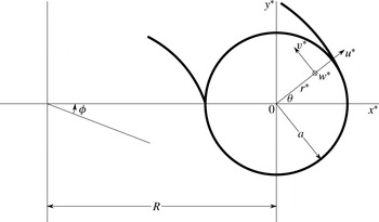
Coordinate system for a curved pipe with circular cross-section of radius
 $a$
and large curvature radius
 $R$
.

We consider steady fully developed incompressible flow of a Newtonian fluid with viscosity
 $\unicode[STIX]{x1D707}$
and density
 $\unicode[STIX]{x1D70C}$
down a weakly curved circular pipe of radius
 $a$
driven by a down-pipe pressure gradient,
 $G$
. We take local Cartesian
 $(x^{\ast },y^{\ast })$
and polar coordinates
 $(r^{\ast },\unicode[STIX]{x1D703})$
at the pipe centre as shown in figure 1, where the superscript
 $^{\ast }$
denotes a dimensional variable. It should be noted that the angle
 $\unicode[STIX]{x1D703}$
is defined differently in BM. The radius of the pipe centreline is
 $R$
, where
 $a\ll R$
, and
 $\unicode[STIX]{x1D719}$
is the angular down-pipe coordinate. The velocity components in the
 $r^{\ast },\unicode[STIX]{x1D703}$
and
 $\unicode[STIX]{x1D719}$
directions are
 $u^{\ast },v^{\ast }$
and
 $w^{\ast }$
respectively, and for fully developed flow these are independent of
 $\unicode[STIX]{x1D719}$
. We adopt the non-dimensional variables
 $$\begin{eqnarray}r^{\ast }=ar,\quad u^{\ast }=\frac{\unicode[STIX]{x1D708}}{a}u,\quad v^{\ast }=\frac{\unicode[STIX]{x1D708}}{a}v,\quad w^{\ast }=w_{0}w,\end{eqnarray}$$
where
 $w_{0}=a^{2}G/(4\unicode[STIX]{x1D707})$
is the maximal velocity that would be driven in a straight pipe by the same pressure gradient and
 $\unicode[STIX]{x1D708}=\unicode[STIX]{x1D707}/\unicode[STIX]{x1D70C}$
is the kinematic viscosity. In addition, we introduce the streamfunction
 $\unicode[STIX]{x1D713}$
to satisfy the continuity equation, such that
 $u=\unicode[STIX]{x1D713}_{\unicode[STIX]{x1D703}}/r$
and
 $v=-\unicode[STIX]{x1D713}_{r}$
. The small-curvature Dean limit is obtained by letting
 $(a/R)\rightarrow 0$
and defining the Dean number,
 $K=(2a/R)(aw_{0}/\unicode[STIX]{x1D708})^{2}$
, following Dean (Reference Dean1928). We obtain the dimensionless Dean equations
 $$\begin{eqnarray}\displaystyle & \unicode[STIX]{x1D6FB}^{4}\unicode[STIX]{x1D713}={\mathcal{J}}(\unicode[STIX]{x1D6FB}^{2}\unicode[STIX]{x1D713},\unicode[STIX]{x1D713})-Kww_{y}, & \displaystyle\end{eqnarray}$$
 $$\begin{eqnarray}\displaystyle & \unicode[STIX]{x1D6FB}^{2}w={\mathcal{J}}(w,\unicode[STIX]{x1D713})-4, & \displaystyle\end{eqnarray}$$
where
 $$\begin{eqnarray}\unicode[STIX]{x1D6FB}^{2}f=\frac{\unicode[STIX]{x2202}^{2}f}{\unicode[STIX]{x2202}r^{2}}+\frac{1}{r}\frac{\unicode[STIX]{x2202}f}{\unicode[STIX]{x2202}r}+\frac{1}{r^{2}}\frac{\unicode[STIX]{x2202}^{2}f}{\unicode[STIX]{x2202}\unicode[STIX]{x1D703}^{2}},\quad {\mathcal{J}}(f,g)=\frac{1}{r}\left(\frac{\unicode[STIX]{x2202}f}{\unicode[STIX]{x2202}r}\frac{\unicode[STIX]{x2202}g}{\unicode[STIX]{x2202}\unicode[STIX]{x1D703}}-\frac{\unicode[STIX]{x2202}f}{\unicode[STIX]{x2202}\unicode[STIX]{x1D703}}\frac{\unicode[STIX]{x2202}g}{\unicode[STIX]{x2202}r}\right).\end{eqnarray}$$
Finally, we impose the solid-wall boundary conditions, requiring that at
 $r=1$
,
 $$\begin{eqnarray}w=\frac{\unicode[STIX]{x2202}\unicode[STIX]{x1D713}}{\unicode[STIX]{x2202}r}=\unicode[STIX]{x1D713}=0.\end{eqnarray}$$
The Dean equations (2.2) and (2.3) have the up–down symmetry
 $\unicode[STIX]{x1D703}\mapsto -\unicode[STIX]{x1D703}$
,
 $\unicode[STIX]{x1D713}\mapsto -\unicode[STIX]{x1D713}$
, which is preserved in all solutions. As we will be considering all complex values of the Dean number
 $K$
, it is useful to note the following additional invariances.
 $$\begin{eqnarray}I_{1}:\quad \unicode[STIX]{x1D703}\rightarrow \unicode[STIX]{x03C0}-\unicode[STIX]{x1D703},\quad K\mapsto -K,\quad w\mapsto w,\quad \unicode[STIX]{x1D713}\rightarrow -\unicode[STIX]{x1D713}.\end{eqnarray}$$
 $$\begin{eqnarray}I_{2}:\quad K\mapsto \overline{K},\quad w\mapsto \overline{w},\quad \unicode[STIX]{x1D713}\rightarrow \overline{\unicode[STIX]{x1D713}}.\end{eqnarray}$$
Here,
 $I_{1}$
corresponds to reflection in
 $x=0$
inverting the inside and outside of the bend, and
 $I_{2}$
to complex conjugation.
3 Solution methods
We adopt two techniques to study complex solutions of the Dean equations: DNS and analytic continuation of series expansions using high-order approximants (HOAs). Details were given in BM, which we summarise below.
3.1 Direct Navier–Stokes simulation
To solve the Dean equations (2.2) and (2.3) numerically, we use a spectral decomposition in
 $\unicode[STIX]{x1D703}$
and second-order central differences in the radial direction,
 $$\begin{eqnarray}w(r_{j},\unicode[STIX]{x1D703})=\mathop{\sum }_{k=0}^{\unicode[STIX]{x1D705}}W_{k}(r_{j})\cos (k\unicode[STIX]{x1D703}),\quad \unicode[STIX]{x1D713}(r_{j},\unicode[STIX]{x1D703})=\mathop{\sum }_{k=1}^{\unicode[STIX]{x1D705}}\unicode[STIX]{x1D6F9}_{k}(r_{j})\sin (k\unicode[STIX]{x1D703}),\end{eqnarray}$$
where
 $r_{j}=j/(M+1)$
for
 $0\leqslant j\leqslant M+1$
are the radial gridpoints. The truncation parameter
 $\unicode[STIX]{x1D705}$
and number of gridpoints
 $M$
are varied to ensure adequate resolution. In contrast to BM, for numerical efficiency we here restrict attention with this decomposition to flows that are symmetric about the
 $x$
axis,
 $$\begin{eqnarray}w(r,\unicode[STIX]{x1D703})=w(r,-\unicode[STIX]{x1D703}),\quad \unicode[STIX]{x1D713}(r,\unicode[STIX]{x1D703})=-\unicode[STIX]{x1D713}(r,-\unicode[STIX]{x1D703}).\end{eqnarray}$$
No steady solutions, real or complex, violating this constraint have been found, although some of the real four-vortex solutions are known to be unstable to time-dependent symmetry-breaking perturbations (Daskopoulos & Lenhoff Reference Daskopoulos and Lenhoff1989).
The resulting algebraic system is solved by path continuation in the parameter
 $K$
, which may be complex. Bifurcation points are traversed using pseudo-arclength and branch-switching techniques. As we shall see, due to the localised structures on some of these solution branches, the resolution required varies greatly across the complex branches studied. For each solution presented here, the robustness has been verified and the resolution used is specified.
3.2 Series extension and analytic continuation by HOAs
Following Van Dyke (Reference Van Dyke1974), we construct the Dean series of the solution, an expansion in powers of
 $K$
,
 $$\begin{eqnarray}w(r,\unicode[STIX]{x1D703})=\mathop{\sum }_{n=0}^{\infty }w_{n}(r,\unicode[STIX]{x1D703})K^{n}\quad \text{and}\quad \unicode[STIX]{x1D713}(r,\unicode[STIX]{x1D703})=\mathop{\sum }_{n=0}^{\infty }\unicode[STIX]{x1D713}_{n}(r,\unicode[STIX]{x1D703})K^{n},\end{eqnarray}$$
with the leading-order term being Poiseuille flow in a straight pipe,
 $$\begin{eqnarray}w_{0}(r,\unicode[STIX]{x1D703})=1-r^{2}\quad \text{and}\quad \unicode[STIX]{x1D713}_{0}(r,\unicode[STIX]{x1D703})=0.\end{eqnarray}$$
On substituting the series into (2.2) and (2.3) and collecting in powers of
 $K$
, we find that as
 $n$
increases,
 $\unicode[STIX]{x1D713}_{n}(r,\unicode[STIX]{x1D703})$
and
 $w_{n}(r,\unicode[STIX]{x1D703})$
satisfy a sequence of successively more complicated linear problems in the lower-order coefficients which can be represented as recurrence relations and solved exactly to all orders. Schematically,
 $w_{n}\sim \sum E_{nij}r^{j}\cos (\text{i}\unicode[STIX]{x1D703})$
. At order
 $n$
, roughly
 $n^{3}$
coefficients need to be found. In total, approximately
 $10^{7}$
coefficients have been calculated up to
 $n=196$
using an arbitrary precision package in
 $\text{C}^{++}$
(Free Software Foundation 2013).
It is convenient to pick a global quantity as a measure for the flow. Here, we adopt the flux ratio,
 $Q$
, defined as the integral of
 $w$
over the pipe cross-section divided by the flux in a straight pipe. It only involves even values of
 $n\equiv 2m$
and its series has the form
 $$\begin{eqnarray}Q=\mathop{\sum }_{m=0}^{\infty }a_{m}(K^{2})^{m},\quad \text{where}~a_{m}=\mathop{\sum }_{j=0}^{7m+1}\frac{2E_{2m0j}}{j+1}.\end{eqnarray}$$
The coefficient array
 $E_{nij}$
is given in BM and we have calculated the coefficients up to
 $a_{98}$
. Another reference quantity used is
 $\unicode[STIX]{x1D6FA}$
, the total vorticity in the upper semicircle, or equivalently the integral of the velocity along
 $y=0$
.
We now use the high-order Hermite–Padé approximant method of Drazin & Tourigny (Reference Drazin and Tourigny1996) to find multiple solutions of the Dean equations and to analytically continue the series beyond its radius of convergence. Truncating (3.5) to
 $N$
terms, the idea is to construct polynomial expressions in
 $Q$
and
 $K$
of increasing order,
 $d$
, which have (3.5) as one of their roots. Sometimes, other roots of these polynomials appear and persist as
 $d$
increases. These are identified as other possible solution branches.
We define the function
 $S(K)=Q(K)-a_{0}$
, so that
 $S(0)=0$
. From (3.5),
 $S(K)$
has the truncated series representation
 $$\begin{eqnarray}S_{N}(K)=\mathop{\sum }_{n=1}^{N}a_{n}(K^{2})^{n}=S(K)+O(K^{2N+2})\quad \text{as}~K\rightarrow 0.\end{eqnarray}$$
We then assume that
 $S(K)$
is an algebraic function of
 $K$
and so seek a polynomial of degree
 $d\geqslant 2$
in two variables
 $F_{d}(K,s)$
, which we write as
 $$\begin{eqnarray}F_{d}(K,s)=\mathop{\sum }_{l=1}^{d}\mathop{\sum }_{m=0}^{l}f_{l-m,m}(K^{2})^{l-m}s^{m}.\end{eqnarray}$$
We find the coefficients
 $f_{i,j}$
by imposing that
 $s=S_{N}(K)$
be an approximate solution,
 $$\begin{eqnarray}F_{d}(K,S_{N}(K))=O(K^{2N+2})\quad \text{as}~K\rightarrow 0.\end{eqnarray}$$
For definiteness, we fix
 $f_{0,1}=1$
and set
 $N=(d^{2}+3d-2)/2$
to ensure the same number of unknown coefficients as defining equations in (3.8).
The polynomial equation
 $F_{d}=0$
will have
 $d$
solutions for
 $s$
. These are found and traced as
 $K$
varies using standard path continuation techniques in MAPLE. By construction, one branch approximates an analytic continuation of the known solution
 $s=S_{N}(K)$
in the classical manner of Hermite–Padé approximants. Some of the remaining
 $d-1$
branches will be spurious, as identified by their transient nature as
 $d$
is increased. However, those solution branches that persist as
 $d$
increases are assumed to approximate new solutions which somewhere bifurcate from the main branch
 $s=S(K)$
(Drazin & Tourigny Reference Drazin and Tourigny1996). Thus, even though we start with a series representation of a single-valued function, the HOA continuation method can predict the emergence of multiple solutions, as well as extending the main solution beyond its circle of convergence. An identical process may be performed with
 $\unicode[STIX]{x1D6FA}$
and, more laboriously, with the series representations of the entire flow
 $(\unicode[STIX]{x1D713},w)$
at every gridpoint. Once the existence of a new solution branch is indicated by the HOA, it can be confirmed using DNS, which requires a good initial estimate to converge. Continuation techniques within DNS are then used to follow the solution branches outside the region where the HOA is reliable.
4 Constructing complex solution branches
We will soon find that for
 $K\not =0$
there are multiple complex solutions, even when
 $K$
is real and positive. The solution space is difficult to visualise. Even when we represent the flow with the single parameter
 $Q$
, the solutions
 $Q(K)$
form hypersurfaces in a four-dimensional space when we permit
 $K$
and
 $Q$
to be complex. If two solutions lie on the same hypersurface, then it should be possible to move from one to the other by continuously varying
 $K$
. We are naturally most interested in real
 $K>0$
and real solutions. New real solutions can be sought on a solution hypersurface by seeking to minimise the imaginary component. For Dean flow, there are the main ‘two-vortex’ and ‘four-vortex’ solution branches, which are believed not to bifurcate from each other for any real
 $K$
. We shall now investigate whether it is possible to locate the four-vortex solution from the main solution branch by continuously varying complex
 $K$
.
To aid visualisation, bearing in mind the known bifurcation at imaginary
 $K$
(see BM), we shall usually consider real values of
 $K^{2}$
and plot
 $\text{Re}(Q)$
. Sometimes, we will wish to move through complex
 $K$
-space. Then, we shall keep
 $|K|$
constant, to limit the discussion to three dimensions.
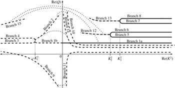
Schematic representation of the bifurcation diagram for
 $Q(K^{2})$
, where the dashed lines represent a pair of complex solutions and the solid lines a single purely real solution. To four significant figures,
 $K_{1}=585.8$
,
 $K_{2}=5.712\times 10^{4}$
and
 $K_{3}=3.888\times 10^{5}$
. On branches 1b, 2, 9 and 15, the imaginary part of
 $w$
and the real part of
 $\unicode[STIX]{x1D713}$
are left–right anti-symmetric. Branches 1–4 and 14 are predicted by HOA, the others by continuation and DNS. The dotted lines denote smooth linkage in complex
 $K$
, keeping
 $|K|$
constant.

In figure 2, we show schematically a portion of the bifurcation diagram found. It incorporates branches 1–8, which are solutions found in previous studies (McConalogue & Srivastava Reference McConalogue and Srivastava1968; Daskopoulos & Lenhoff Reference Daskopoulos and Lenhoff1989; Machane Reference Machane2010; Boshier & Mestel Reference Boshier and Mestel2014) and reproduced here, and branches 9–15, which are found for the first time in the current work. To ease visualisation, the diagram represents branches projected onto the real
 $K^{2}$
axis. The solid lines denote fully real solutions. The branches with dashed lines are complex solutions, although for symmetry reasons the integral
 $Q$
is in fact real on branches 1b, 2, 9 and 15. The HOA technique predicts branches 1–4 and 14, which are then extended using DNS and continuation in the complex parameter
 $K$
. Each complex branch may in fact represent up to four solutions in the fully complex
 $K$
-space related by invariances (2.6) and (2.7). The dotted lines in the figure represent solution paths along circles of constant
 $|K|$
, as described below.
Branches 1a and 1b correspond to the characteristic two-vortex solution found from the analytic Dean series (3.5). Branches 5–8 are the well-known four-vortex solutions, with 5–6 corresponding to those first reported by McConalogue & Srivastava (Reference McConalogue and Srivastava1968) and 7–8 those given by Daskopoulos & Lenhoff (Reference Daskopoulos and Lenhoff1989). The four-vortex solutions can be constructed numerically for large
 $K$
by using an
 $O(1)$
perturbation off branch 1 as a starting point – until now, they have not been locatable in a continuous manner. Once such a solution is found, the branch can be followed down to the bifurcation points at
 $K=K_{2}$
or
 $K_{3}$
, below which they become complex. Branches 2–4 bifurcate from branch 1 at the square-root singularity at
 $K^{2}=-K_{1}^{2}$
, which limits the radius of convergence of the Dean series. Notably, branch 2 is a complex solution, with real flux, on which
 $w$
scales as
 $|K|^{-1/2}$
as
 $K\rightarrow 0$
(BM). It follows that as
 $K\rightarrow 0$
along branch 2, the forcing term
 $-4$
in (2.3) becomes negligible, and the solution approaches an unforced complex solution, which we call an eigensolution.
We now discuss the properties of the new branches and the means by which they were found.
4.1 Eigensolutions of the unforced Dean equations
In BM, we concluded that a solution of the form of branch 2 exists provided that there is a complex solution to the unforced Dean equations
 $$\begin{eqnarray}\displaystyle & \unicode[STIX]{x1D6FB}^{4}\unicode[STIX]{x1D713}={\mathcal{J}}(\unicode[STIX]{x1D6FB}^{2}\unicode[STIX]{x1D713},\unicode[STIX]{x1D713})-Kw(\cos \unicode[STIX]{x1D703}w_{\unicode[STIX]{x1D703}}/r+\sin \unicode[STIX]{x1D703}w_{r}), & \displaystyle\end{eqnarray}$$
 $$\begin{eqnarray}\displaystyle & \unicode[STIX]{x1D6FB}^{2}w={\mathcal{J}}(w,\unicode[STIX]{x1D713}). & \displaystyle\end{eqnarray}$$
Here, we observe that in addition to invariances (2.6) and (2.7), the unforced equations (4.1) and (4.2) have the following invariance.
 $$\begin{eqnarray}I_{3}:\quad K\mapsto \frac{K}{\unicode[STIX]{x1D6FC}^{2}},\quad w\mapsto \unicode[STIX]{x1D6FC}w,\quad \unicode[STIX]{x1D713}\rightarrow \unicode[STIX]{x1D713},\end{eqnarray}$$
where
 $\unicode[STIX]{x1D6FC}\in \mathbb{C}$
is a constant. It is clear that by choosing a suitable constant
 $\unicode[STIX]{x1D6FC}$
, the eigensolution for
 $K^{2}<0$
can be transformed to a complex solution for real and positive
 $K$
. The forced solution is a perturbation of this scaled eigensolution. We therefore infer the existence of solution branches 9–11 from their known asymptotic forms as
 $K\rightarrow 0$
. Good initial estimates to the solutions near
 $K=0$
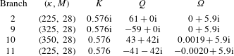
on branches 9–11 can be found by scaling the branch-2 solution, and all four branches closely approximate the unforced solution. As
 $K\rightarrow 0$
, the solution hypersurface resembles a funnel about
 $K=0$
, along which
 $|Q|\sim Q_{0}/|K|^{1/2}$
.
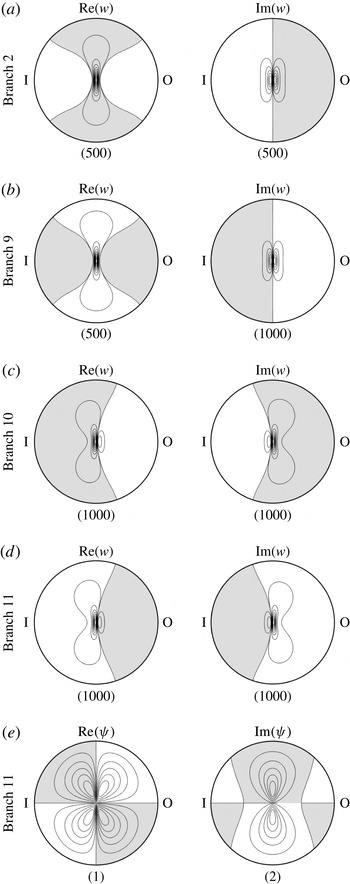
Contour plots of
 $w$
near
 $K=0$
, which approximate the ‘eigensolution’: (a) branch 2,
 $(\unicode[STIX]{x1D705},M)=(28,225)$
, and (b) branch 9,
 $(\unicode[STIX]{x1D705},M)=(28,325)$
, both at
 $K=0.576\text{i}$
; (c) branch 10,
 $(\unicode[STIX]{x1D705},M)=(28,350)$
, and (d) branch 11,
 $(\unicode[STIX]{x1D705},M)=(28,350)$
, at
 $K=0.576$
. (e) The streamfunction
 $\unicode[STIX]{x1D713}$
on branch 11, which is indistinguishable from
 $\unicode[STIX]{x1D713}$
on the other branches. The numbers in brackets denote the contour interval, I/O indicate the inside/outside of the bend.

Explicitly, we construct close initial approximations to solutions of the full Dean equations (2.2) and (2.3) by applying (4.3) to solutions on branch 2,
 $(w,\unicode[STIX]{x1D713},K)=(w_{2},\unicode[STIX]{x1D713}_{2},\text{i}k)$
, where
 $|k|\ll 1$
. Specifically, branch 9 is found with an initial approximation
 $(-w_{2},\unicode[STIX]{x1D713}_{2},\text{i}k)$
, branch 10 is constructed from the initial estimate
 $(\sqrt{\text{i}}w_{2},\unicode[STIX]{x1D713}_{2},k)$
and branch 11 from
 $(-\sqrt{\text{i}}w_{2},\unicode[STIX]{x1D713}_{2},k)$
. The iteration procedure then locates precise solutions for the full problem. The contour plots of
 $w$
on these branches are shown in figure 3(a–d). For small
 $|K|$
, the solutions are almost images of each other. The corresponding plots for
 $\unicode[STIX]{x1D713}$
are virtually indistinguishable across these branches and so only that of branch 11 is shown in figure 3(e). Corresponding values of
 $Q$
and
 $\unicode[STIX]{x1D6FA}$
are given in table 1. The solution patterns diverge as
 $|K|$
increases.
As expected, on branch 9, the imaginary part of
 $w$
and the real part of
 $\unicode[STIX]{x1D713}$
are left–right anti-symmetric. This is not the case for branches 10 and 11. A common feature of all of the branches is that as
 $K$
varies, they may develop a localised structure. On branch 9, the localisation is symmetric about the origin and is well resolved by our polar decomposition, but this is less so for the solutions on branches 10–14 where the symmetry is broken. The development of these structures means that following solutions can become computationally expensive. For example, a converged solution at
 $K=10^{-3}$
on branch 10 requires a typical resolution
 $(\unicode[STIX]{x1D705},M)=(28,325)$
, while for
 $K=5.184\times 10^{4}$
we need
 $(\unicode[STIX]{x1D705},M)=(24,525)$
, and increasing
 $K$
is laborious. As we shall see, it is more fruitful to follow paths for complex
 $K$
-values.
4.2 Path continuation in real
 $K$

In light of complex bifurcation theory (Henderson & Keller Reference Henderson and Keller1990), we expect complex solutions to bifurcate from the four-vortex solutions at
 $K_{2}=5.712\times 10^{4}$
and
 $K_{3}=3.888\times 10^{5}$
. As these are simple turning points for complex
 $K$
, branches 12 and 13 are found by branch-switching at
 $K_{2}$
and
 $K_{3}$
respectively. Two complex solution branches that exist at
 $K<K_{2}$
and
 $K<K_{3}$
coalesce and become real at these points.
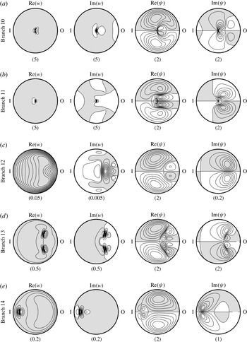
Contour plots of the azimuthal velocity
 $w$
and the streamfunction
 $\unicode[STIX]{x1D713}$
at
 $K=5.184\times 10^{4}$
: (a) branch 10,
 $(\unicode[STIX]{x1D705},M)=(24,525)$
; (b) branch 11,
 $(\unicode[STIX]{x1D705},M)=(28,450)$
; (c) branch 12,
 $(\unicode[STIX]{x1D705},M)=(28,250)$
; (d) branch 13,
 $(\unicode[STIX]{x1D705},M)=(48,250)$
; (e) branch 14,
 $(\unicode[STIX]{x1D705},M)=(24,225)$
.

Flux
 $Q$
and upper vorticity
 $\unicode[STIX]{x1D6FA}$
for solutions near
 $K=0$
, as in figure 3.
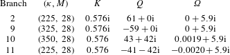
Flux
 $Q$
and upper vorticity
 $\unicode[STIX]{x1D6FA}$
for solutions at
 $K=5.184\times 10^{4}$
, corresponding to figure 4.
Five different complex solutions are plotted for
 $K=5.184\times 10^{4}$
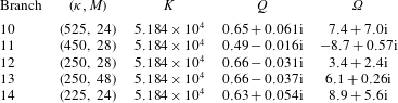
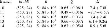
in figure 4. They exhibit great differences in structure. The relative sizes of the real and imaginary parts suggest that branch 12 is closest to hitting a real solution, as is indeed the case. The double-dipole structure exhibited in
 $w$
on branch 13 is quite distinct from all other solutions found, and it is possible that this solution lies on a separate hypersurface from the others. The values of
 $Q$
and
 $\unicode[STIX]{x1D6FA}$
pertaining to these five flows are given in table 2.
Ideally, we would like to be able to follow the complex solutions on branches 12 and 13 to
 $K=0$
, or connect them to any of the other branches that stem from the singular eigensolution. Unfortunately, we find that as
 $K$
is kept real and reduced, the solutions develop a localised structure, making them computationally difficult to resolve. Thus, for example, branch 12 is troublesome for
 $K<1.152\times 10^{4}$
. Investigation in complex
 $K$
-space reveals the proximity of another more structured complex solution branch, which can be circumvented by choosing a different path. This characteristic is visible in figure 4(e). Accordingly, we turn our attention to constructing paths for fully complex
 $K$
.
4.3 Path continuation in complex
$K$

Selection of the best path to follow in complex
 $K$
-space to connect known branches is not trivial. In practice, we have limited our consideration to arcs of constant
 $|K|$
which are chosen so as to avoid regions where the solutions are difficult to resolve. Such arcs are indicated by dotted lines in figure 2. The direction we take on these paths, anti-clockwise or clockwise round the imaginary
 $K$
-axis, is also chosen to avoid any solution that develops localised structures. In this manner, we have been able to identify new branches for real
 $K$
as well as joining already identified branches in complex
 $K$
-space. Thus, for example, moving round the
 $K=0$
axis connects branch 9 to branch 11 in a straightforward manner, while branches 3 and 4 join with the real branch 1a. The behaviour from branch 2 is less obvious and may result in either branch 10 or 14 because of the proximity to a highly structured branch.
Branch 15 at
 $K=-5.76\times 10^{4}\text{i}$
,
 $(\unicode[STIX]{x1D705},M)=(125,16)$
.

Contours of
 $w$
and
 $\unicode[STIX]{x1D713}$
for (a)
 $K=5760$
,
 $(\unicode[STIX]{x1D705},M)=(225,40)$
; (b)
 $K=5120-2602\text{i}$
,
 $(\unicode[STIX]{x1D705},M)=(325,16)$
; (c)
 $K=1920-5462\text{i}$
,
 $(\unicode[STIX]{x1D705},M)=(150,16)$
; (d)
 $K=-5760\text{i}$
,
 $(\unicode[STIX]{x1D705},M)=(125,16)$
, see figure 5; (e)
 $K=5120-7926\text{i}$
,
 $(\unicode[STIX]{x1D705},M)=(125,16)$
; (f)
 $K=11199-6075\text{i}$
,
 $(\unicode[STIX]{x1D705},M)=(125,16)$
; (g)
 $K=14400\text{i}$
,
 $(\unicode[STIX]{x1D705},M)=(125,16)$
. Panels (a–d) link branches 10 and 15 along
 $|K|=5760$
; (e–g) link branches 15 and 12 along
 $|K|=14400$
.

We now construct a continuous solution path joining the complex eigensolution branch 10 with branch 12. This path includes two circular arcs in complex
 $K$
-space. We start on branch 10 at
 $K=5.76\times 10^{3}$
, a point chosen to lie well within the region where branch 10 is easy to resolve. The circle
 $|K|=5.76\times 10^{4}$
is then followed anti-clockwise up to
 $K=-5.76\times 10^{3}\text{i}$
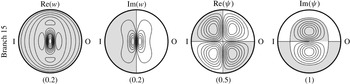
. Here, we find a new solution branch 15. This branch has the same symmetry characteristics as branches 1, 2 and 9, in that the flux is real and the total vorticity in the upper semicircle is imaginary, as can be inferred from figure 5. Were we to continue anti-clockwise further on this circle, we would encounter a region where solutions become difficult to resolve before reaching real
 $K$
again. Instead, we follow branch 15 to
 $K=-1.44\times 10^{4}\text{i}$
. At this point, we follow the circle
 $|K|=1.44\times 10^{4}$
in a clockwise manner. We find that this path has no difficulty in constructing solutions up to
 $K=1.44\times 10^{4}$
, where we reach branch 12, a safe distance from the value near
 $K=1.152\times 10^{4}$
which causes trouble. Hence, with these two arcs, we form a continuous path which joins our eigensolution branch 10 to branch 12, the complex solution that bifurcates from the four-vortex solutions at
 $K=K_{2}$
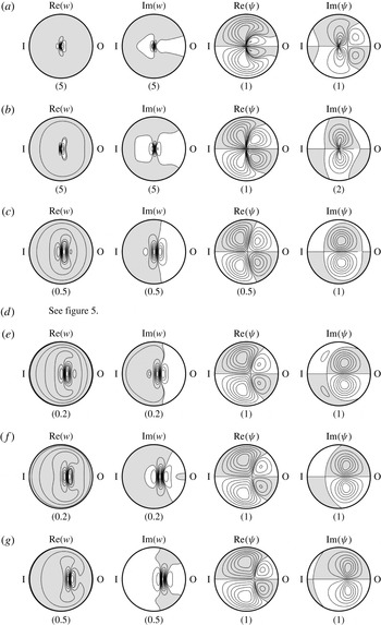
. Sample solutions along this path are shown in figure 6. Panels (a–c) link onto figure 5 along
 $|K|=5.76\times 10^{3}$
, while (e–g) link branches 12 and 15 along
 $|K|=1.44\times 10^{4}$
.
We have thus achieved our goal of linking the real four-vortex solution branches 5 and 6 to the main solution branch 1. A continuous solution path runs respectively through the complex branches 2, 10, 15 and 12, joining via semicircles in complex values of
 $K^{2}$
. Despite some effort, we have been unable to link branches 7 and 8 via branch 13 to the main solution tree in this manner, and it is possible that the second ‘four-vortex’ solution branch in fact lies on a disjoint complex hypersurface. The double-dipole nature of figure 6(e) is quite different from the structures seen on the other branches.
Despite this success, we cannot really claim that our branch-tracking procedure provides a cost-effective way to predict the real multi-vortex solutions for this problem. Nevertheless, the existence of such a path provides encouragement regarding the value of studying the Navier–Stokes equations in the full complex domain. Other problems with more solution branches have provided a more fruitful application of the procedures employed in this paper, for example Vaz, Boshier & Mestel (Reference Vaz, Boshier and Mestel2017).
5 Pipes of elliptic cross-section
Dean flows in circular pipes have received by far the most attention in the literature, although rectangular and triangular ducts have also been considered. We now briefly report on Dean flow in pipes of elliptic cross-section with various aspect ratios. As expected, this problem is found to exhibit many features similar to those of the circular pipe. Machane (Reference Machane2010) found multi-vortex solutions for elliptic cross-sections of aspect ratio
 $\unicode[STIX]{x1D706}=1.45$
, although his bifurcation diagram differs from that found for the circular cross-section. Interestingly, in his study, he concluded that the number of vortices on a particular branch may gradually change without running through a singular point, suggesting that ‘number of vortices’ is not a robust diagnostic for distinguishing between solutions in the elliptic case.
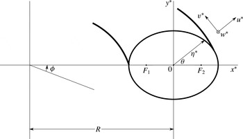
Coordinate system for a curved pipe with elliptic cross-section; foci at
 $F_{1}=R-a$
and
 $F_{2}=R+a$
, and radius of centreline
 $R$
.

We take local coordinates at the pipe centre, as shown in figure 7, where the superscript
 $^{\ast }$
denotes a dimensional variable. The Cartesian and elliptic coordinates are related by
 $x^{\ast }=a\cosh \unicode[STIX]{x1D702}\cos \unicode[STIX]{x1D703}$
,
 $y^{\ast }=a\sinh \unicode[STIX]{x1D702}\sin \unicode[STIX]{x1D703}$
. The boundary at
 $\unicode[STIX]{x1D702}=\unicode[STIX]{x1D702}_{0}$
is an ellipse with foci at
 $x^{\ast }=\pm a$
and corresponding aspect ratio
 $\unicode[STIX]{x1D706}=\tanh \unicode[STIX]{x1D702}_{0}$
. We note that as
 $\unicode[STIX]{x1D702}_{0}\rightarrow \infty$
,
 $\unicode[STIX]{x1D706}\rightarrow 1$
, and in this limit the cross-section is a circle of infinite radius. Thus, our scaling keeps a fixed distance between the two foci, rather than, say, fixing the perimeter or the area of the ellipse. The velocity components in the
 $\unicode[STIX]{x1D702}$
,
 $\unicode[STIX]{x1D703}$
and
 $\unicode[STIX]{x1D719}$
directions are
 $u^{\ast }$
,
 $v^{\ast }$
and
 $w^{\ast }$
respectively, and for fully developed flow these are independent of
 $\unicode[STIX]{x1D719}$
. We adopt the non-dimensional variables
 $$\begin{eqnarray}\unicode[STIX]{x1D6FE}=\frac{\unicode[STIX]{x1D6FE}^{\ast }}{a\cosh \unicode[STIX]{x1D702}_{0}},\quad u=\frac{\unicode[STIX]{x1D708}u^{\ast }}{a\cosh ^{2}\unicode[STIX]{x1D702}_{0}},\quad v=\frac{\unicode[STIX]{x1D708}v^{\ast }}{a\cosh ^{2}\unicode[STIX]{x1D702}_{0}},\quad w=\frac{w^{\ast }}{w_{0}},\end{eqnarray}$$
where the scale factor
 $\unicode[STIX]{x1D6FE}^{\ast }=a\sqrt{\cosh 2\unicode[STIX]{x1D702}-\cos 2\unicode[STIX]{x1D703}}$
,
 $w_{0}$
is the maximal azimuthal velocity driven in a straight pipe by the same pressure gradient and
 $\unicode[STIX]{x1D708}$
is the kinematic viscosity. The continuity equation is satisfied by introducing a streamfunction
 $\unicode[STIX]{x1D713}$
such that
 $u=\unicode[STIX]{x1D713}_{\unicode[STIX]{x1D703}}/\unicode[STIX]{x1D6FE}$
and
 $v=-\unicode[STIX]{x1D713}_{\unicode[STIX]{x1D702}}/\unicode[STIX]{x1D6FE}$
. The dimensionless Dean equations are then
 $$\begin{eqnarray}\displaystyle & \unicode[STIX]{x1D6FB}^{2}w={\mathcal{J}}(\unicode[STIX]{x1D713},w)-2(1+\coth ^{2}\unicode[STIX]{x1D702}_{0}), & \displaystyle\end{eqnarray}$$
 $$\begin{eqnarray}\displaystyle & \displaystyle \unicode[STIX]{x1D6FB}^{4}\unicode[STIX]{x1D713}={\mathcal{J}}(\unicode[STIX]{x1D713},\unicode[STIX]{x1D6FB}^{2}\unicode[STIX]{x1D713})-K\frac{w}{\unicode[STIX]{x1D6FE}^{2}}\left(\frac{\cosh \unicode[STIX]{x1D702}\sin \unicode[STIX]{x1D703}}{\cosh \unicode[STIX]{x1D702}_{0}}\frac{\unicode[STIX]{x2202}w}{\unicode[STIX]{x2202}\unicode[STIX]{x1D702}}+\frac{\sinh \unicode[STIX]{x1D702}\cos \unicode[STIX]{x1D703}}{\cosh \unicode[STIX]{x1D702}_{0}}\frac{\unicode[STIX]{x2202}w}{\unicode[STIX]{x2202}\unicode[STIX]{x1D703}}\right), & \displaystyle\end{eqnarray}$$
 $$\begin{eqnarray}\unicode[STIX]{x1D6FB}^{2}f=\frac{1}{\unicode[STIX]{x1D6FE}^{2}}\left(\frac{\unicode[STIX]{x2202}^{2}f}{\unicode[STIX]{x2202}\unicode[STIX]{x1D702}^{2}}+\frac{\unicode[STIX]{x2202}^{2}f}{\unicode[STIX]{x2202}\unicode[STIX]{x1D703}^{2}}\right)\quad \text{and}\quad {\mathcal{J}}(f,g)=\frac{1}{\unicode[STIX]{x1D6FE}^{2}}\left(\frac{\unicode[STIX]{x2202}f}{\unicode[STIX]{x2202}\unicode[STIX]{x1D703}}\frac{\unicode[STIX]{x2202}g}{\unicode[STIX]{x2202}\unicode[STIX]{x1D702}}-\frac{\unicode[STIX]{x2202}f}{\unicode[STIX]{x2202}\unicode[STIX]{x1D702}}\frac{\unicode[STIX]{x2202}g}{\unicode[STIX]{x2202}\unicode[STIX]{x1D703}}\right).\end{eqnarray}$$
The Dean number now takes the form
 $K=2a^{3}w_{0}^{2}\cosh ^{3}\unicode[STIX]{x1D702}_{0}/(\unicode[STIX]{x1D708}^{2}R)$
. Finally, we impose the solid-wall boundary condition and require that at
 $\unicode[STIX]{x1D702}=\unicode[STIX]{x1D702}_{0}$
,
 $$\begin{eqnarray}w=\frac{\unicode[STIX]{x2202}\unicode[STIX]{x1D713}}{\unicode[STIX]{x2202}\unicode[STIX]{x1D702}}=\unicode[STIX]{x1D713}=0.\end{eqnarray}$$
We can also use the above equations to consider pipes with aspect ratio
 $\unicode[STIX]{x1D706}>1$
by applying the transformation
 $$\begin{eqnarray}\unicode[STIX]{x1D702}\rightarrow \unicode[STIX]{x1D702}+\text{i}\frac{\unicode[STIX]{x03C0}}{2}\quad \text{and}\quad a\rightarrow -\text{i}a.\end{eqnarray}$$
We are therefore able to examine flows in ducts varying continuously between very squat (
 $\unicode[STIX]{x1D706}\rightarrow 0$
) and very tall (
 $\unicode[STIX]{x1D706}\rightarrow \infty$
) cross-sections. The solutions pass smoothly through the circular case
 $\unicode[STIX]{x1D706}=1$
.
5.1 Small and large
$\unicode[STIX]{x1D706}$

For small
 $\unicode[STIX]{x1D706}$
, the top and bottom boundaries are close and almost parallel, so that
 $\unicode[STIX]{x1D713}$
and
 $w$
are expected to be independent of
 $x$
near the centre of the pipe. To leading order in
 $\unicode[STIX]{x1D706}$
, the Dean equations (5.2a
) and (5.2b
) reduce to
 $$\begin{eqnarray}\frac{\text{d}^{2}w}{\text{d}y^{2}}=-\frac{2}{\unicode[STIX]{x1D706}^{2}}+O(1),\quad \frac{\text{d}^{4}\unicode[STIX]{x1D713}}{\text{d}y^{4}}=-\frac{K}{2}w\frac{\text{d}w}{\text{d}y},\end{eqnarray}$$
with solution
 $$\begin{eqnarray}w=1-\frac{y^{2}}{\unicode[STIX]{x1D706}^{2}}\quad \text{and}\quad \unicode[STIX]{x1D713}=\frac{K\unicode[STIX]{x1D706}^{3}}{840}\left(1-\frac{y^{2}}{\unicode[STIX]{x1D706}^{2}}\right)^{2}\left(5-\frac{y^{2}}{\unicode[STIX]{x1D706}^{2}}\right)\frac{y}{\unicode[STIX]{x1D706}}.\end{eqnarray}$$
This solution is in accordance with the rectangular Dean–Hele-Shaw flow considered by Mestel & Zabielski (Reference Mestel and Zabielski2012), in the context of dynamo theory. It was shown that at moderately high Reynolds number, the above flow was prone to an inflection-point type of instability, but that does not concern us here.
For large
 $\unicode[STIX]{x1D706}$
, we approach the thin-gap limit of Taylor–Couette flow. To leading order,
 $\unicode[STIX]{x1D713}$
and
 $w$
are expected to be independent of
 $y$
near the centre of the pipe. In this case, the Dean equations (5.2a
) and (5.2b
) are solved to leading order by plane Poiseuille flow,
 $$\begin{eqnarray}w=1-x^{2}\quad \text{and}\quad \unicode[STIX]{x1D713}=0.\end{eqnarray}$$
The secondary cross-pipe flow is driven by the distant horizontal boundaries, and is small in the main body of the pipe.
5.2 Numerical methods
We use a similar method to that for the circular cross-section, which is adaptable for real or complex solutions. We use a spectral decomposition in
 $\unicode[STIX]{x1D703}$
and finite differences on the grid
 $\unicode[STIX]{x1D702}=\unicode[STIX]{x1D702}_{j}\equiv j\unicode[STIX]{x1D702}_{0}/J$
for
 $j=1\ldots J$
,
 $$\begin{eqnarray}\unicode[STIX]{x1D713}(\unicode[STIX]{x1D702}_{j},\unicode[STIX]{x1D703})=\mathop{\sum }_{k=-\unicode[STIX]{x1D705}}^{\unicode[STIX]{x1D705}}f_{j,k}\text{e}^{\text{i}k\unicode[STIX]{x1D703}},\quad w(\unicode[STIX]{x1D702}_{j},\unicode[STIX]{x1D703})=\mathop{\sum }_{k=-\unicode[STIX]{x1D705}}^{\unicode[STIX]{x1D705}}w_{j,k}\text{e}^{\text{i}k\unicode[STIX]{x1D703}}.\end{eqnarray}$$
When constructing the numerical scheme for (5.2a
) and (5.2b
), we must be careful near the two coordinate singularities at the foci
 $F_{1}$
and
 $F_{2}$
or
 $\unicode[STIX]{x1D702}=0$
,
 $\unicode[STIX]{x1D703}=0$
,
 $\unicode[STIX]{x03C0}$
, where
 $\unicode[STIX]{x1D6FE}=0$
. Care is also required on the line
 $\unicode[STIX]{x1D702}=0$
joining the foci, providing a boundary condition on the finite differencing. We require continuity of
 $w$
,
 $\unicode[STIX]{x1D713}$
and
 $\unicode[STIX]{x1D6FB}^{2}\unicode[STIX]{x1D713}$
across this line. We ensure this by introducing fictitious points at
 $j=-1$
and note that
 $w$
is top–bottom symmetric while
 $\unicode[STIX]{x1D713}$
and
 $\unicode[STIX]{x1D6FB}^{2}\unicode[STIX]{x1D713}$
are top–bottom anti-symmetric. For
 $\unicode[STIX]{x1D706}<1$
, this requires, for instance, that
 $w_{-1,k}=w_{1,-k}$
, which we build into the finite difference scheme. In contrast, for
 $\unicode[STIX]{x1D706}>1$
, after using the transformation (5.5), the appropriate condition is
 $w_{-1,k}=(-1)^{k}w_{1,-k}$
.
Path continuation techniques are used as before to follow solution branches.
5.3 Extended series solution and HOAs
Analogously to the circular pipe, we construct the Dean series
 $$\begin{eqnarray}w(\unicode[STIX]{x1D702},\unicode[STIX]{x1D703})=\mathop{\sum }_{n=0}^{\infty }w_{n}(\unicode[STIX]{x1D702},\unicode[STIX]{x1D703})K^{n}\quad \text{and}\quad \unicode[STIX]{x1D713}(\unicode[STIX]{x1D702},\unicode[STIX]{x1D703})=\mathop{\sum }_{n=0}^{\infty }\unicode[STIX]{x1D713}_{n}(\unicode[STIX]{x1D702},\unicode[STIX]{x1D703})K^{n}\end{eqnarray}$$
and find that
 $w_{n}$
and
 $\unicode[STIX]{x1D713}_{n}$
take the forms
 $$\begin{eqnarray}\displaystyle & \displaystyle w_{n}=\mathop{\sum }_{i=0}^{I_{n}}\mathop{\sum }_{j=0}^{I_{n}}E_{nij}(\unicode[STIX]{x1D702}_{0})\left\{\begin{array}{@{}ll@{}}\cosh (2j\unicode[STIX]{x1D702})\cos (2i\unicode[STIX]{x1D703}),\quad & n~\text{even},\\ \cosh ((2j+1)\unicode[STIX]{x1D702})\cos ((2i+1)\unicode[STIX]{x1D703}),\quad & n~\text{odd},\end{array}\right. & \displaystyle\end{eqnarray}$$
 $$\begin{eqnarray}\displaystyle & \displaystyle \unicode[STIX]{x1D713}_{n}=\mathop{\sum }_{i=0}^{J_{n}}\mathop{\sum }_{j=0}^{J_{n}}C_{nij}(\unicode[STIX]{x1D702}_{0})\left\{\begin{array}{@{}ll@{}}\sinh (2j\unicode[STIX]{x1D702})\sin (2i\unicode[STIX]{x1D703}),\quad & n~\text{even},\\ \sinh ((2j+1)\unicode[STIX]{x1D702})\sin ((2i+1)\unicode[STIX]{x1D703}),\quad & n~\text{odd},\end{array}\right. & \displaystyle\end{eqnarray}$$
where
 $J_{n}=7n/2$
for even
 $n$
,
 $J_{n}=(7n-1)/2$
for odd
 $n$
and
 $I_{n}=J_{n}+1$
. The coefficients
 $E_{nij}$
and
 $C_{nij}$
are constant for a given ellipse and can once more be found precisely to all orders. The leading term solves (5.2a
), (5.2b
) when
 $K=0$
and is Poiseuille flow in a straight elliptic pipe,
 $$\begin{eqnarray}\displaystyle & \displaystyle w_{0}(\unicode[STIX]{x1D702},\unicode[STIX]{x1D703})=\frac{(\cosh 2\unicode[STIX]{x1D702}_{0}-\cosh 2\unicode[STIX]{x1D702})(\cosh 2\unicode[STIX]{x1D702}_{0}-\cos 2\unicode[STIX]{x1D703})}{\sinh ^{2}2\unicode[STIX]{x1D702}_{0}}, & \displaystyle\end{eqnarray}$$
 $$\begin{eqnarray}\displaystyle & \unicode[STIX]{x1D713}_{0}(\unicode[STIX]{x1D702},\unicode[STIX]{x1D703})=0. & \displaystyle\end{eqnarray}$$
Subsequent terms for a given value of
 $n$
can be expressed as recurrence relations involving the known coefficients for smaller values of
 $n$
. While the series could be constructed for general
 $\unicode[STIX]{x1D706}$
, in practice, the storage required by the coefficients is prohibitive, and it is best to obtain new series for particular values of
 $\unicode[STIX]{x1D706}$
. Using an arbitrary precision GMP package in
 $\text{C}^{++}$
, coefficients up to
 $n=100$
have been found for
 $\unicode[STIX]{x1D706}=0.4$
, 0.5, 0.75, 0.80, and, by applying transformation (5.5), for
 $\unicode[STIX]{x1D706}=1.25$
, 1.5, 1.75, 2.
As before, we use as a diagnostic the flux ratio
 $Q$
defined as the integral of
 $w$
over the cross-section divided by the flux down a straight pipe with the same cross-section. We derive its series from (5.10) and find that it involves only even powers of
 $K$
,
 $$\begin{eqnarray}Q(K)=\mathop{\sum }_{n=0}^{\infty }\frac{a_{n}}{a_{0}}K^{2n},\end{eqnarray}$$
where
 $$\begin{eqnarray}\displaystyle a_{n} & = & \displaystyle \mathop{\sum }_{j\neq 1}^{Jn}\frac{\unicode[STIX]{x03C0}}{2}\left(\frac{\sinh (2(j-1)\unicode[STIX]{x1D702}_{0})}{2(j-1)}+\frac{\sinh (2(j+1)\unicode[STIX]{x1D702})}{2(j+1)}\right)E_{n0j}-\mathop{\sum }_{j=1}^{Jn}\frac{\unicode[STIX]{x03C0}}{4j}\sinh (2j\unicode[STIX]{x1D702}_{0})E_{n1j}\nonumber\\ \displaystyle & & \displaystyle +\,\frac{\unicode[STIX]{x03C0}}{2}\left(\unicode[STIX]{x1D702}_{0}+\frac{\sinh 4\unicode[STIX]{x1D702}_{0}}{4}\right)E_{n01}-\frac{\unicode[STIX]{x03C0}}{2}\unicode[STIX]{x1D702}_{0}E_{n10}.\end{eqnarray}$$
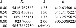
For more details, see Tettamanti (Reference Tettamanti2012). Using Domb–Sykes analysis on the series for the flux
 $Q$
as in Van Dyke (Reference Van Dyke1974), we have found that for every
 $\unicode[STIX]{x1D706}$
, the circle of convergence is limited by square-root singularities at the imaginary values
 $K=\pm \text{i}K_{c}$
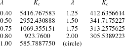
. The behaviour of
 $K_{c}(\unicode[STIX]{x1D706})$
is shown in table 3. The value of the singularity varies with
 $\unicode[STIX]{x1D706}$
, as one might expect, but while as
 $\unicode[STIX]{x1D706}\rightarrow 0$
the radius of convergence of the series increases without bound, it appears to plateau as
 $\unicode[STIX]{x1D706}$
increases beyond 1. In interpreting this, it should be borne in mind that
 $K$
has been defined to keep the focal separation
 $a$
constant.
Radius of convergence
 $K_{c}$
for different aspect ratios
 $\unicode[STIX]{x1D706}$
.
The HOAs up to
 $d=7$
have been constructed for each of the above
 $\unicode[STIX]{x1D706}$
values. This is a lower-order approximant than we had available for the circular cross-section. Nevertheless, we find that these approximants are able to identify reliably a bifurcation diagram equivalent to branches (1a, b, 2–4) found for the circular cross-section. We can conclude that the square-root singularities at
 $K=\pm \text{i}K_{c}$
are also of the symmetry-breaking type found for the circular case and discussed in BM. This leads to a branch 2 that asymptotes towards
 $K=0$
, with the resultant complex eigenfunction. This, in turn, implies the existence of complex solutions for real
 $K>0$
. Complex solutions are believed to exist in all cases for
 $K>0$
, although unlike for the circle, we have calculated insufficient coefficients for the HOAs to predict these explicitly. Nevertheless, the DNS locates them without trouble based on the scaled branch-2 solution.
The eigenfunction takes a fairly simple form for high-aspect-ratio ellipses. As
 $\unicode[STIX]{x1D706}\rightarrow \infty$
, the shape approaches an unbounded pipe with walls at
 $x=\pm 1$
, for which we can find an unforced complex solution to the problem
 $$\begin{eqnarray}J(\unicode[STIX]{x1D713},\unicode[STIX]{x1D6FB}^{2}\unicode[STIX]{x1D713})=\unicode[STIX]{x1D6FB}^{4}\unicode[STIX]{x1D713},\quad \text{with}~\unicode[STIX]{x1D735}\unicode[STIX]{x1D713}=0~\text{on}~x=\pm 1.\end{eqnarray}$$
As the unforced streamfunction has left/right symmetry, we seek a solution of the form
 $\unicode[STIX]{x1D713}=yf(x)$
, where
 $$\begin{eqnarray}f^{\prime }f^{\prime \prime }-ff^{\prime \prime \prime }=f^{\prime \prime \prime \prime },\quad \text{with}~f(\pm 1)=0=f^{\prime }(\pm 1).\end{eqnarray}$$
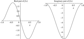
The solution to this homogeneous problem is shown in figure 8. As
 $w=0$
for this solution, it is an example of an unforced complex solution to the two-dimensional Navier–Stokes equation. An essentially identical unforced solution can be found as
 $\unicode[STIX]{x1D706}\rightarrow 0$
.
The real and imaginary parts of the unforced complex flow between two parallel plates, the limit of a high-aspect-ratio ellipse. The streamfunction is
 $\unicode[STIX]{x1D713}=yf(x)$
or
 $\unicode[STIX]{x1D713}=xf(y)$
.

In summary, so far as we are able to discern, the solution structure for ellipses of moderate aspect ratio appears to resemble closely that of the circle. Unforced solutions exist, as do complex solutions for real
 $K$
.
6 Concluding remarks
In this paper, we have demonstrated that the unforced solution for small but imaginary Dean number found in BM automatically leads to complex solutions for real positive
 $K$
. The existence of such extra complex solution branches has not previously been reported, but has now been found in other simple problems. Indeed, we conjecture that such solutions are usually, if not always, present for the Navier–Stokes equations. With hindsight, their existence is very plausible. A complex velocity field does not have the same energetic limitations as a physical real flow, and need not require a forcing term. An unforced flow, whose magnitude is proportional to the viscosity, satisfies a fully nonlinear PDE effectively at intermediate Reynolds number,
 $$\begin{eqnarray}\boldsymbol{u}\boldsymbol{\cdot }\unicode[STIX]{x1D735}\boldsymbol{u}=-\unicode[STIX]{x1D735}\boldsymbol{p}+\unicode[STIX]{x1D6FB}^{2}\boldsymbol{u},\quad \unicode[STIX]{x1D735}\boldsymbol{\cdot }\boldsymbol{u}=0.\end{eqnarray}$$
That such a nonlinear problem should possess a complex solution is no great surprise. A further plausibility argument can be advanced for domains with a symmetry plane, say at
 $x=0$
. If we introduce an imaginary coordinate
 $\unicode[STIX]{x1D709}=\text{i}x$
, then the elliptic Laplacian operator becomes hyperbolic in terms of
 $(\unicode[STIX]{x1D709},y,z)$
and a real unforced solution to that problem would raise no eyebrows, although mathematically it corresponds to a complex unforced solution to the Navier–Stokes equations in real space.
Granted that extra complex solutions to the forced Navier–Stokes equations exist, one can nevertheless question the practical worth of finding and studying them. Leaving aside any insight that might in time derive from a better understanding of the full complex solution space, our intended justification is to understand and perhaps predict bifurcations to new physical solutions, which may come into being at the junction of two complex solution branches. In this paper, we have demonstrated that the first pair of four-vortex solutions to the Dean equations can be continuously linked onto the unforced eigensolution at
 $K=0$
, and thence onto the main solution branch and its analytic continuation. Reversing the process, the four-vortex solution branch could have been located continuously, rather than by using slightly arbitrary initial conditions for DNS.
Yet, the authors would be the first to admit that for this problem at least, the effort required to locate and predict the four-vortex solution was disproportionately intensive. If
 $K$
and the diagnostic parameter
 $Q$
are regarded as complex, the solution space for
 $Q(K)$
may ‘only’ be four-dimensional, but it is nevertheless difficult to navigate and comprehend, partly because it conceals much of the structure of the full PDE solution. We have not presented here all of the complex solutions found and have, indeed, in our numerical investigations, sometimes striven to avoid those with more intricate structure.
A natural question to ask is whether the techniques described here, the pioneering work of Van Dyke, computationally extended 100-fold and viewed through the prismatic HOA lens of Drazin & Tourigny (Reference Drazin and Tourigny1996), can be recommended for other problems.
Inevitably, this is hard to answer. The HOA method is very good at locating bifurcations off the main solution branch, but could not predict subcritical bifurcations from infinity, such as the four-vortex solutions. It was natural to expect for our problem that the complex solution branches known to exist for
 $K$
slightly positive would merge directly as
 $K$
increased with the complex branches known to exist for
 $K<K_{2}$
. However, the behaviour was more complex in our study and it is difficult to predict what will happen in general. The techniques have, however, already been applied with some success to problems in convection and planetary dynamics which are known to possess more prominent bifurcations. In the former case, the singularity limiting the convergence of the Stokes series was found to correspond to a physical hysteresis at real Grashof number. The method led directly to the discovery of other real solution branches (Vaz et al.
Reference Vaz, Boshier and Mestel2017). Calculations have also been performed for the flow between concentric rotating spheres.
It is, of course, also possible to investigate complex solutions without going through the Stokes series/HOA route. An unforced solution to (6.1) depends only on geometry and, once it is known, it can be used as the same numerical starting point for path continuation of complex solutions to problems with varied physical forcing. Whether or not as the Reynolds number is increased these complex solutions will end in coalescence at real bifurcations will depend on the forcing in the particular problem, but in our view it is certainly worth investigating.
Acknowledgement
The authors would like to thank A. Thomas for his help with setting up the numerical infrastructure for this work.