1. INTRODUCTION
With the development of Micro Electro Mechanical System (MEMS) technology, low-cost magnetometers and Inertial Navigation Systems (INS) can be integrated into a module or chip. The integration is widely used in many applications, such as indoor navigation, human body motion tracking and Attitude Heading Reference Systems (AHRS) for unmanned aerial vehicles and the like (Wu et al., Reference Wu, Yao, Ma and Jia2013; Yadav and Bleakley, Reference Yadav and Bleakley2014; Yun et al., Reference Yun, Aparicio, Bachmann and McGhee2005; Cui et al., Reference Cui, Mei, Qin, Yan and Fu2017; Foxlin, Reference Foxlin2005). An INS usually includes gyroscopes and accelerometers. A MEMS gyroscope can measure the angular velocity of a vehicle, but it is usually unable to sense the local rotational angular velocity of the Earth. So, it is hard to achieve self-alignment with a MEMS gyroscope. A magnetometer can measure local magnetic field and an accelerometer can measure the acceleration, which can be used to calculate the attitudes of the system, but these attitudes are discrete. Hence, the integration of magnetometer and INS is commonly used to provide continuous and stable attitudes (Huang et al., Reference Huang, Zhou, Zhang, Yang, Song, Chen and Zhang2018; Wahdan et al., Reference Wahdan, Georgy and Noureldin2015 and Sarkka et al., Reference Sarkka, Nieminen, Suuriniemi and Kettunen2017). However, magnetometers are prone to be influenced by magnetic disturbances, and they must be calibrated in advance.
The existing calibration methods for a magnetometer can be divided into two parts, off-line and on-line. Ellipsoid fitting is a representative method to calibrate a magnetometer off-line (Fang et al., Reference Fang, Sun, Cao, Zhang and Tao2011]; Olivares et al., Reference Olivares, Ruiz-Garcia, Olivares, Gorriz and Ramirez2013 and Zhu et al., Reference Zhu, Zhao, Cheng and Zhou2017). The advantages of this method are simplicity and a lower calculation burden, but it has also the shortcoming of low precision. The particle swarm optimisation algorithm is a new off-line magnetometer calibration method (Wu et al., Reference Wu, Wu, Hu and Wu2011; Riwanto et al., Reference Riwanto, Tikka, Kestila and Praks2017). It can utilise a more accurate nonlinear model and need not consider the initial estimation parameters. The calibration precision is improved, but it also increases the calculation burden. For on-line calibration, “attitude-independent” is a classic method (Huang and Jing, Reference Huang and Jing2008; Grandvallet et al., Reference Grandvallet, Zemouche, Boutayeb and Changey2014; Draganová et al., Reference Draganová, Laššák, Praslièka and Kán2014; Wu and Wang, Reference Wu and Wang2018). By removing the attitude matrix, this method achieves calibration using only the outputs of the magnetometer. In order to improve calibration accuracy and reduce computation burden, many filters are used such as Extended Kalman Filter (EKF) (Grandvallet et al., Reference Grandvallet, Zemouche, Boutayeb and Changey2014), neural network and so on (Draganová et al., Reference Draganová, Laššák, Praslièka and Kán2014; Wu and Wang, Reference Wu and Wang2018). Recently, integrated calibration methods combining magnetometer and INS have been developed (Wu et al., Reference Wu, Zou, Liu and Yu2018b). By using the characteristics of magnetometers and gyroscopes, this method realises the simultaneous calibration of both. However, the above calibration methods are only suitable for constant magnetic disturbance and pre-calibration before use, that is to say, they cannot deal with random magnetic disturbances during use.
There are many methods to deal with unknown random interference, such as adaptive filters (Cai et al., Reference Cai, Xing, Zhang and Shen2017), robust control and so on (Liu et al., Reference Liu, Sun, Ye and Shi2017; Qian et al., Reference Qian, Huang, Qian and Shen2014). For random magnetic disturbance, a Kalman filter with a two-step observation update has been proposed (Gao et al., Reference Gao, Wang and Zhao2017), but the disturbance was not analysed in detail and only sudden disturbances were considered. A novel online magnetic disturbance estimator using nonlinear programming has been proposed (Wu, Reference Wu2019), however, it mainly solves the problem of static estimation of unknown outer magnetic disturbances, rather than variable random magnetic disturbances in dynamic motion. Besides, this method is mainly motivated by aligning the magnetically distorted attitude quaternion to a better reference that can be provided by inertial/Global Navigation Satellite System (GNSS)/visual/Lidar sensors, but the reference quaternion is hard to obtain for integration that only includes a magnetometer and an INS. Based on the above method, an adaptive anti-disturbance method for magnetometer and INS integration is proposed. The main contributions of this method are as follows:
(1) By analysing the actual data from driving tests, different kinds of disturbances are found and classified. Then, the corresponding solution is presented.
(2) The magnetometer's update model using angular velocity from a gyroscope is deduced, and at the same time, an Adaptive Robust Extended Kalman Filter (AREKF) is designed to overcome sudden disturbances.
(3) A fast magnetometer calibration method is proposed for long-term disturbances. When a long-term disturbance occurs, an AREKF can maintain precision during the early stage, at the same time, the magnetic fields from an AREKF can be used to calibrate the magnetometer.
(4) Data from simulation and an actual driving test are used to verify the effectiveness of the proposed method.
The rest of this paper is organised as follows. Section 2 introduces the classification and disturbance analysis results and then the corresponding solution is proposed. In Section 3, the formulation is presented. The results of simulations and the driving test are shown in Sections 4 and 5. Section 6 concludes the paper.
2. DISTURBANCE ANALYSIS
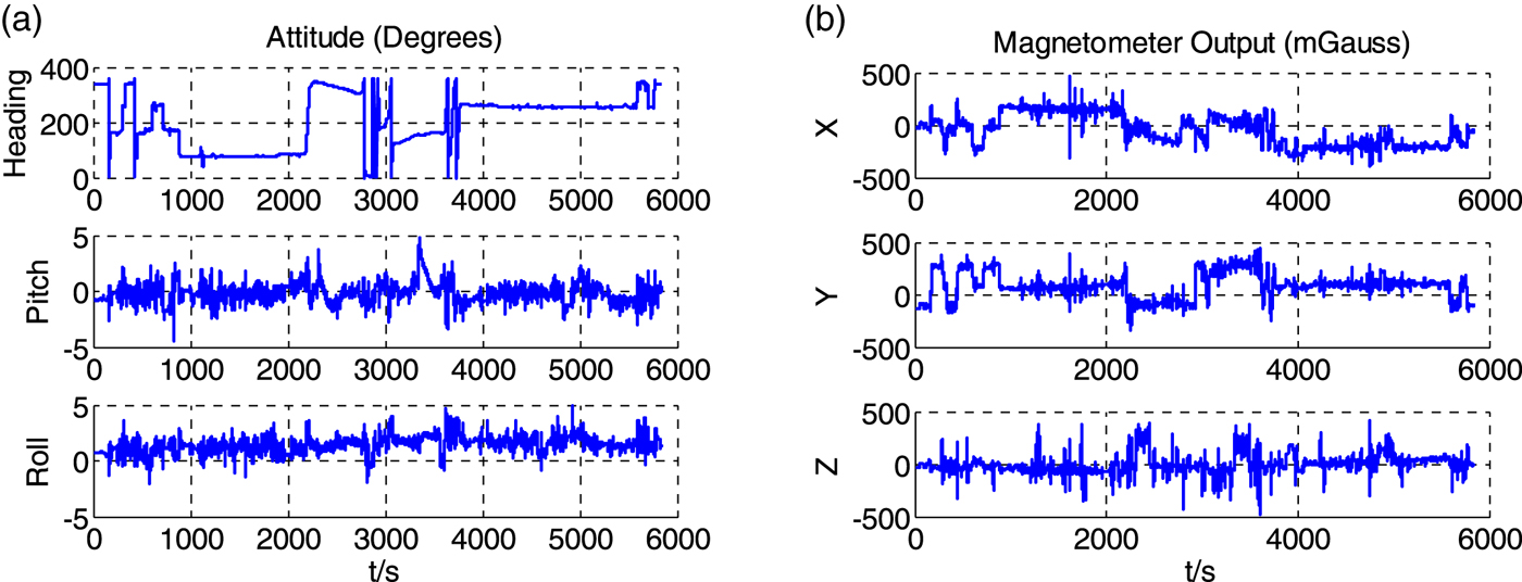
In this section, magnetic disturbance is discussed and analysed from the data of an actual driving test. This driving test was carried out in the city and the equipment included a high precision attitude reference system and a MEMS-INS system. These two systems were fixed in the vehicle and the data was collected synchronously. In Figure 1, the attitudes of the vehicle are provided by a high precision attitude reference system and the magnetometer outputs are obtained from MEMS-INS.
(a) Attitude of the vehicle. (b) Output of the magnetometer.

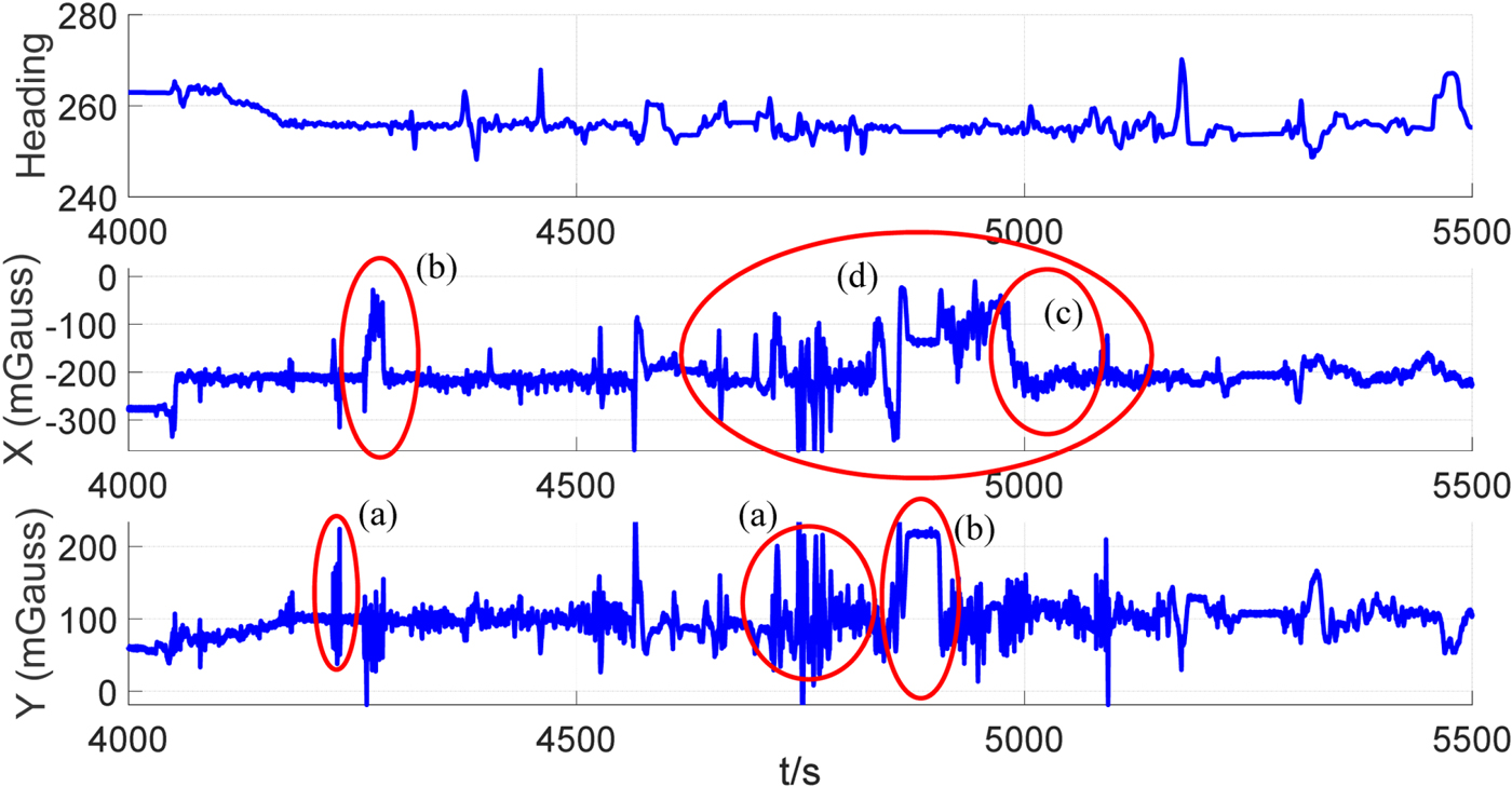
To recognise the disturbance, data from 4,000 to 5,500 seconds are analysed. Due to the heading being primarily related to the output of the magnetometer in x and, y-axes, the heading angle and output of the magnetometer in x and y-axes are shown in Figure 2.
The comparison of heading angle and output of magnetometer in x and y axes.

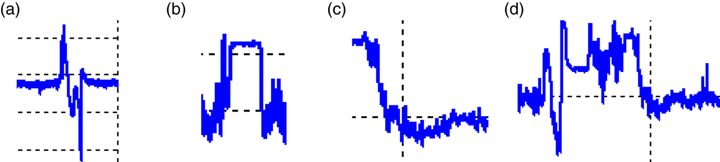
From Figure 2, the change of heading angle remains within 20°; in other words, the road vehicle is basically moving around a straight line but the magnetometer's outputs go over 100 mGauss every now and then. Some typical magnetic perturbations have been marked by red ellipses in Figure 2. Based on Figure 2, these perturbations are classified into four types and this is shown in Figure 3. Descriptions of these perturbations are summarised as follows:
Disturbance (a): When Disturbance (a) occurs, there is a large noise but the mean of noise has little change as shown in Figure 3(a). This perturbation may be caused by a car quickly passing by the magnetometer.
Disturbance (b): When Disturbance (b) occurs, the outputs of the magnetometer have a step change and hold for some time as shown in Figure 3(b). This perturbation may be caused by the situation that the vehicle causing the perturbation remains close to the side of the magnetometer.
Disturbance (c): When Disturbance (c) occurs, the outputs of the magnetometer slowly change and hold for some time as shown in Figure 3(c). This perturbation may be caused by the situation that the adjacent vehicle causing the perturbation slowly closes the magnetometer.
Disturbance (d): Figure 3(d) is a combination of the above perturbations.These different kinds of disturbance are caused by complex road conditions, such as passing nearby cars or moving through or beside buildings.
The different kinds of disturbance.

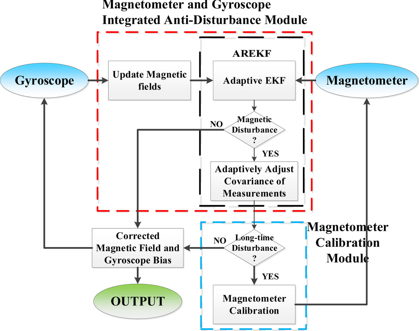
For solving these disturbances, an adaptive robust cascaded Kalman filter is proposed in this paper and the flow diagram for the filter is shown in Figure 4.
A flow diagram of the proposed method.

The proposed method is divided into two modules, the magnetometer and gyroscope integrated anti-disturbance module and a magnetometer calibration module. In the magnetometer and gyroscope integrated anti-disturbance module, the magnetic fields are updated first by gyroscope and then the updated results are put into the AREKF module to adaptively filter sudden disturbances. When a magnetic disturbance appears, the time of disturbance will be evaluated to determine whether the magnetometer needs to be calibrated. If a long-term disturbance is determined, the magnetometer calibration module will start-up and then the results of magnetometer calibration will be substituted into the update model of the magnetometer for the next anti-disturbance process.
3. METHOD FORMULATION
In this section, the specific details of sub-modules will be introduced. The frame is determined as follows:
(1) Navigation frame (n-frame): The origin of navigation frame is located on the vehicle and its x, y and z axes respectively point to the east, north and upward.
(2) Body frame (b-frame): The body frame follows the right-hand rule. Its x and y axes point to the right and front of the vehicle.
3.1. Integrated anti-disturbance module
3.1.1. Magnetometer and gyroscope model
When a disturbance occurs, the outputs of the magnetometer have errors, but they can be maintained by angular velocity from the gyroscope. Based on this idea, the magnetometer model using angular velocity from the gyroscope needs to be deduced first. The magnetometer measurement model can be expressed as (Wu and Wang, Reference Wu and Wang2018):
 $${\bf B}_m^{b_k} ={\bf C}_{sc} {\bf C}_{no} \lpar {\bf C}_{si} {\bf C}_n^{b_k } {\bf B}_t^n +{\bf b}_{bi} \rpar +{\bf b}_b +{\brvarepsilon}_m $$
where  ${\bf B}_{m}^{b_{k}}$ is the output from the magnetometer at step k in the b-frame.
 ${\bf B}_{t}^{n}$ is the true magnetic field in the n-frame and it can be obtained from the International Geomagnetic Reference Field (IGRF) model (Finlay et al., Reference Finlay, Maus, Beggan, Alken, Aubert, Barrois, Bertrand, Bondar, Boness, Brocco, Canet, Chambodut, Chulliat, Coïsson, Civet, Du, Fournier, Fratter, Gillet, Hamilton, Hamoudi, Hulot, Jager, Korte, Kuang, Lalanne, Langlais, Léger, Lesur, Lowes, Macmillan, Mandea, Manoj, Maus, Olsen, Petrov, Ridley, Rother, Sabaka, Saturnino, Schachtschneider, Sirol, Tangborn, Thomson, Tøffner-Clausen, Vigneron, Wardinski and Zvereva2010).
 ${\bf C}_{n}^{b_{k}}$ is the rotation matrix from the n-frame to the b-frame at step k. bbi and bb are the hard-iron effect and bias vector.
 ${\brvarepsilon}_{m}$ is the measurement noise and is Gaussian white noise. Csi, Csc and Cno represent the soft-iron matrix, scale factor matrix and non-orthogonal matrix, respectively. Their expressions are shown as follows:
 $${\bf C}_{si} = \left[{\matrix{ {C_{six} } & {C_{sixy} } & {C_{sixz} } \cr {C_{siyx} } & {C_{siy} } & {C_{siyz} } \cr {C_{sizx} } & {C_{sizy} } & {C_{siz} } \cr }} \right]$$
 $${\bf C}_{sc} = \left[{\matrix{ {C_{scx} } & 0 & 0 \cr 0 & {C_{scy} } & 0 \cr 0 & 0 & {C_{scz} } \cr } } \right]$$
 $${\bf C}_{no} =\left[{\matrix{ 0 & {C_{noxy} } & {C_{noxz} } \cr {C_{noyx} } & 0 & {C_{noyz} } \cr {C_{nozx} } & {C_{noyz} } & 0 \cr } } \right]$$
For convenience, the model can be re-written as:
 $${\bf B}_m^{b_k } ={\bf C}_m {\bf C}_n^{b_k } {\bf B}_t^n +{\bf b}_m +{\brvarepsilon}_m $$
in which:
 $${\bf C}_m = {\bf C}_{sc} {\bf C}_{no} {\bf C}_{si} $$
 $${\bf b}_m = {\bf C}_{sc} {\bf C}_{no} {\bf b}_{bi} +{\bf b}_b $$
Based on Equation (5), the model at step k − 1 can be expressed as:
 $${\bf B}_m^{b_{k-1} } ={\bf C}_m {\bf C}_n^{b_{k-1} } {\bf B}_t^n +{\bf b}_m +{\brvarepsilon }_m $$
Hence,  ${\bf C}_{n}^{b_{k-1} } {\bf B}_{t}^{n} $ can be transformed by Equation (8):
 $${\bf C}_n^{b_{k-1} } {\bf B}_t^n ={\bf C}_m^{-1} \lpar {{\bf B}_m^{b_{k-1} } -{\bf b}_m -{\brvarepsilon }_m } \rpar $$
Due to the prior knowledge of attitude update by gyroscope, the relation between  ${\bf C}_{n}^{b_{k}}$ and
 ${\bf C}_{n}^{b_{k-1}}$ can be expressed as (Wu and Wang, Reference Wu and Wang2018):
 $${\bf C}_n^{b_k } =\lpar {{\bf I}_3 -\lsqb {{\bi \omega }_t^{b_k } \times } \rsqb t_s } \rpar {\bf C}_n^{b_{k-1} } $$
where I3 is an identity matrix with three dimensions.  $\lsqb {{\bi \omega }_{t}^{b_{k}} \times}\rsqb $ is an anti-symmetric matrix by the output of gyroscope
 ${\bi \omega }_{t}^{b_{k}}$ at step k and t s is the interval of data update. Combining Equations (5), (9) and (10), the magnetometer model using angular velocity from the gyroscope can be obtained as:
 $${\bf B}_m^{b_k } ={\bf C}_m \lpar {{\bf I}_3 -\lsqb {{\bi \omega }_t^{b_k } \times } \rsqb t_s } \rpar {\bf C}_m^{-1} \lpar {{\bf B}_m^{b_{k-1} } -{\bf b}_m } \rpar +{\bf b}_m +{\brvarepsilon }_m $$
As the magnetometer has been calibrated, Cm and bm of Equation (11) are considered as constant. Then,  ${\bi \omega}_{t}^{b_{k}}$ in Equation (11) can be obtained by gyroscope model.
The gyroscope model can be given as (Wu and Wang, Reference Wu and Wang2018):
 $${\bi \omega }_g^{b_k } ={\bf C}_g {\bi \omega }_t^{b_k } +{\bf b}_g^{b_k } +{\brvarepsilon }_g $$
where  ${\bi \omega }_{g}^{b_{k}}$ is the output of the gyroscope and
 ${\bf b}_{g}^{b_{k}}$ is the gyroscope bias in the b-frame at the step k. Cg is a complex matrix obtained by combining the scale factor matrix, non-orthogonal matrix and misalignment error matrix.
 ${\brvarepsilon}_{g}$ is the output noise of the gyroscope and it is zero-mean Gaussian white noise. An accurately calibrated gyroscope significantly helps the magnetometer update module. In existing methods, some external sources can aid gyroscope calibration, for example, sun sensors, star trackers, polarised light, etc. (Chang et al., Reference Chang, Hu and Li2016; Wu et al., Reference Wu, Zhou, Fourati and Liu2018a). They can also be treated as vector measurements for compensation of a gyroscope's long-term bias. In this paper, considering low-cost navigation systems and calculation burden, a magnetometer is used to calibrate the gyroscope and Cg is considered that it has been calibrated before leaving the factory. So, the gyroscope model can be simplified as follows:
 $${\bi \omega }_g^{b_k } ={\bi \omega}_t^{b_k } +{\bf b}_g^{b_k}+{\brvarepsilon }_g. $$
3.1.2. Adaptive Robust Extended Kalman (AREKF)
This filter is mainly to solve for sudden disturbances, like Disturbance (a) or (b). This filter needs to be able to adaptively adjust its parameters. In existing fusion algorithms for multi-sensor systems, there are many excellent algorithms, which include traditional adaptive filters and robust filters. There is also a new Generalised Linear Quaternion Complementary Filter (Wu et al., Reference Wu, Zhou, Fourati, Li and Liu2019). For convenience, the AREKF is selected in this part. In this filter, the state is selected as the magnetic field and the bias of the gyroscope in the b-frame, that is,  ${\bf x}_{k}^{1} =\lsqb {\bf B}_{m}^{b_{k}} \quad {\bf b}_{g}^{b_{k}}\rsqb ^{T}$. The measurement is the output of magnetometer
 ${\tilde{\bf B}}_{m}^{b_{k}}$, that is,
 ${\bf z}_{k}^{1} ={\tilde {\bf B}}_{m}^{b_{k}}$. The AREKF algorithm is as follows,
(1) Time update:
 $${\bf x}_{k/k-1}^1 =f\lpar {{\bf x}_{k-1}^1 }\rpar $$
 $${\bf P}_{k/k-1} ={\bf \Phi }_{k\comma k-1} {\bf P}_{k-1} {\bf \Phi }_{k\comma k-1}^T +{\bf Q}_k $$
 $${\bf \Phi}_{k,k-1} = \displaystyle{{\partial f\lpar {{\bf x}^1} \rpar }\over{\partial {\bf x}^1}}\lpar {{\bf x}^1={\bf x}_{k-1}^1 }\rpar$$
(2) Innovation covariance estimation:
 $${\bf V}_k = {\bf z}_k^1 -{\bf H}_k {\bf x}_{k/k-1}^1 $$
 $${\bf C}_k = \displaystyle{{1}\over{N}}\sum\limits_{k=k_0 }^N {{\bf V}_k {\bf V}_k^T} $$
(3) Measurement update:
 $$\left\{\matrix{{\bf P}_{zz} ={\bf H}_k {\bf P}_{k/k-1} {\bf H}_k^T +{\bf C}_k \hfill & \hbox{Without magnetic disturbance} \hfill \cr {\bf P}_{zz} ={\bf H}_k {\bf P}_{k/k-1} {\bf H}_k^T + c \ast \max \lpar {\mathop {set}\limits_{i=i_0}^k \lpar {\bf V}_k {\bf V}_k^T \rpar }\rpar \hfill & \hbox{With magnetic disturbance} \hfill \cr}\right. $$
 $${\bf K}_k ={\bf P}_{k/k-1} {\bf H}_k^T {\bf P}_{zz}^{-1} $$
 $${\bf x}_k^1 ={\bf x}_{k/k-1}^1 +{\bf K}_k {\bf V}_k $$
 $${\bf P}_k ={\bf P}_{k/k-1} -{\bf K}_k {\bf P}_{zz} {\bf K}_k^T $$
f(·) is the state transition function and it consists of Equations (11) and (13). The transition process of  ${\bf B}_{m}^{b_{k}}$ is based on Equation (11) and the gyroscope bias
 ${\bf b}_{g}^{b_{k}} = {\bf b}_{g}^{b_{k-1}}$ is considered as constant. Φk,k−1 is the state transition matrix and it can be calculated by f(·). Vk is the residual between prediction and measurement, Ck is the average result of sliding window
 ${\bf V}_{k} {\bf V}_{k}^{T}$ and the window's size is N. In Equation (19), the decision criteria between without magnetic disturbances and with magnetic disturbances is the square root of
 ${\bf V}_{k} {\bf V}_{k}^{T}$, the value of threshold is usually set as two to five times the magnetometer output noise. From Equation (19), EKF is changed to adaptive EKF by taking Ck as the measurement noise covariance matrix without magnetic disturbance, which can increase adaptability and convergence speed. When a magnetic disturbance appears, the maximum value of
 $set\lpar {\bf V}_{k} {\bf V}_{k}^{T}\rpar $ is used as the measurement noise covariance matrix. c is the amplification coefficient and the value of c is based on the features of the magnetometer. For example, if the output noise of the magnetometer is relatively large, the value of c needs to be bigger to highlight the influence of the disturbance, the value of c usually is between 1~10. This solution adds robust control to the adaptive EKF so that it can improve the resistibility for large noise magnetic disturbance.
3.2. Magnetometer calibration module
When Disturbances (b) and (c) in Figures 2 and 3 occur, the disturbance may persist, which could still lead to errors if only using AREKF. Therefore, the magnetometer needs to be quickly calibrated. The attitude-independent method is often used to real-time calibrate magnetometers (Alonso and Schuster, Reference Alonso and Shuster2002; Crassidis et al., Reference Crassidis, Lai and Harman2005; Söken and Sakai, Reference Söken and Sakai2017). This method can calibrate a magnetometer without attitude information but needs representative motion for good observability of the filter and this kind of motion is hard to achieve in a car. Besides, a gyroscope can provide a relatively accurate attitude over a short time. So, attitudes from the gyroscope can be used to quickly calibrate the magnetometer in the early stages of a long-time disturbance. Based on Equation (8), we can get the output model of the magnetometer at step k during a long-time disturbance as follows:
 $$\eqalign{{\bf B}_m^{b_k} & =\lpar {\bf C}_m +{\bf C}_r\rpar {\bf C}_n^{b_k} {\bf B}_t^n +\lpar {\bf b}_m +{\bf b}_r\rpar +{\brvarepsilon}_m \cr & ={\bf C}_m {\bf C}_n^{b_k} {\bf B}_t^n +\lpar {\bf C}_r {\bf C}_n^{b_k} {\bf B}_t^n +{\bf b}_m +{\bf b}_r\rpar +{\brvarepsilon}_m \cr & = {\bf C}_m {\bf C}_n^{b_k} {\bf B}_t^n +{\hat {\bf b}}_m +{\brvarepsilon}_m} $$
 $${\hat{\bf b}}_m = {\bf C}_r {\bf C}_n^{b_k} {\bf B}_t^n +{\bf b}_m +{\bf b}_r $$
where Cr is the scale factor error matrix and br is the bias error vector. When the change of  ${\bf C}_{n}^{b_{k}}$ is small,
 ${\hat{\bf b}}_{m}$ can be considered as approximately constant. Long-term stable disturbances often occur in the static case, such as the situation that the navigation system stops beside a disturbance source. For improving the coverage speed and decreasing the calculation burden, errors caused by disturbances are considered as the bias of the magnetometer, Cm is considered as a calibrated constant parameter before leaving the factory. To sum up, the bias of the magnetometer needs to be calibrated. The magnetometer calibration model from Equation (5) can be given as follows:
(1) State transition model:
(25) $${\dot{\bf b}}_m = 0 $$(26)$$\dot {k}_b = 0 $$
(2) Measurement model:
(27)$${\bf B}_m^{b_k} = {\bf C}_m {\bf C}_n^{b_k} {\bf B}_t^n +{\bf b}_m $$(28)$$\Vert {{\bf B}_m^{b_k}} \Vert =k_b s+ \Vert {{\bf B}_m^{b_k}} \Vert _{0} $$


where  ${\bf B}_{m}^{b_{k}}$ is the output of the magnetometer and Cm is known after initial calibration.
 ${\bf C}_{n}^{b_{k}}$ can be calculated from the results of the AREKF. The slope k b of
 $\Vert {{\bf B}_{m}^{b_{k}}} \Vert $ is related to time and it can be used to distinguish Disturbances (b) or (c). s is the run time and
 $\Vert {\bf B}_{m}^{b_{k}} \Vert _{0}$ is the initial value of
 $\Vert {{\bf B}_{m}^{b_{k}}} \Vert $ at every filtering start. In this filter, the state and measurement vectors are selected as
 ${\bf x}_{k}^{2} =\lsqb { {{\bf b}_{m}} \quad {k_{b}}} \rsqb ^{T}$ and
 ${\bf z}_{k}^{2} =\lsqb {\bf B}_{m}^{b_{k}} \quad \Vert {\bf B}_{m}^{b_{k}} \Vert \rsqb ^{T}$; a standard Kalman Filter (KF) is used.
4. SIMULATION AND ANALYSIS
Due to the existing methods rarely considering random disturbances, this section will analyse the impacts under the different disturbances, and the proposed method will be verified by comparing with other reference methods. This section is divided into three parts, comparative algorithms, simulation data and simulation results.
4.1. Comparative Algorithms
To check the effectiveness of the proposed method, several reference methods are compared as follows.
4.1.1. The standard Extended Kalman Filter (EKF)
EKF is widely used for magnetometer and INS integrated calibration (Wu et al., Reference Wu, Zou, Liu and Yu2018b). In this method, the update function of the attitude matrix and the magnetometer output model are taken as the state transition model. The output of the magnetometer is used as a measurement. Hence the standard EKF system is expressed as follows:
(1) State transition model:
(29)$${\dot{\bf C}}_{b_k }^n = {\bf C}_{b_{k-1} }^n\lpar {{\bi \omega }_t^{b_k }+{\bf b}_g^{b_k } } \rpar \times $$(30)$${\dot{\bf b}}_g^{b_k } = 0 $$(31)$${\dot{\bf b}}_m = 0 $$(32)$${\bf B}_m^{b_k } = {\bf C}_m {\bf C}_n^{b_k } {\bf B}_t^n +{\bf b}_m $$(2) Measurement model:
(33)$${\tilde{\bf B}}_m^{b_k } ={\bf B}_m^{b_k} $$


where  ${\tilde {\bf B}}_{m}^{b_{k} } $ is the output of the magnetometer. Cm is considered as a known constant that has been calibrated before leaving the factory.
4.1.2. The Adaptive Extended Kalman Filter (AEKF)
The AEKF is based on the above standard EKF method and the adaptive process is set to the measurement update of EKF (Fang and Yang, Reference Fang and Yang2011). The detail is as follows:
(1) Measurement update:
(34)$${\bf V}_k = {\bf z}_k^1 -{\bf H}_k {\bf x}_{k/k-1}^1 $$(35)$${\bf C}_k = \displaystyle{{1}\over{N}}\sum\limits_{k=k_0 }^N {{\bf V}_k {\bf V}_k^T} $$(36)$${\bf P}_{zz} ={\bf H}_k {\bf P}_{k/k-1} {\bf H}_k^T +{\bf C}_k $$(37)$${\bf K}_k ={\bf P}_{k/k-1} {\bf H}_k^T {\bf P}_{zz}^{-1} $$(38)$${\bf x}_k^1 ={\bf x}_{k/k-1}^1 +{\bf K}_k {\bf V}_k $$(39)$${\bf P}_k ={\bf P}_{k/k-1} -{\bf K}_k {\bf P}_{zz} {\bf K}_k^T $$


4.1.3. AREKF without magnetometer calibration
AREKF was introduced in Section 3.1.
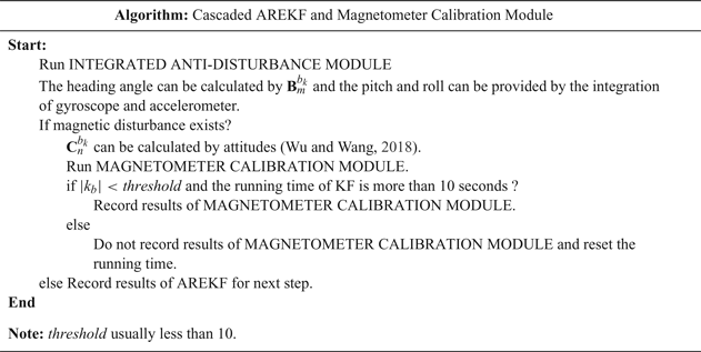
The proposed method combines the advantages of the above method. At the same time, it considers the situation that disturbances may exist for a long time. When any disturbances occur, AREKF will be used to resist them, and then, it we will be judged whether the disturbance is stable and exists for a long time. If so, the magnetometer will be recalibrated using the results from AREKF over a short time, because a gyroscope can only guarantee accuracy over a short time. Then the calibrated parameters will be substituted into the magnetometer model for the next anti-disturbance process. The process of cascading two filters is summarised in Table 1. In this method, the normalisation of the magnetometer's output is used to judge whether the system is disturbed.
The process of cascading two filters.

4.2. Simulation data
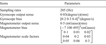
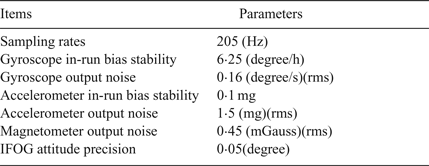
In existing research, representative motions are needed for good filter observability (Fedele et al., Reference Fedele, D'Alfonso and D'Aquila2018; Wu et al., Reference Wu, Zou, Liu and Yu2018b). These representative motions can be used to more accurately calibrate the magnetometer. However, this paper focuses on anti-disturbance technology after calibration and the representative motion is not required. For verifying the performance of the proposed method, two sets of simulation data, sets A and B, were designed using MATLAB. The features of the INS and magnetometer in the simulation are shown in Table 2.
Simulation parameters of INS and Magnetometer system.

4.2.1. Simulation data set A
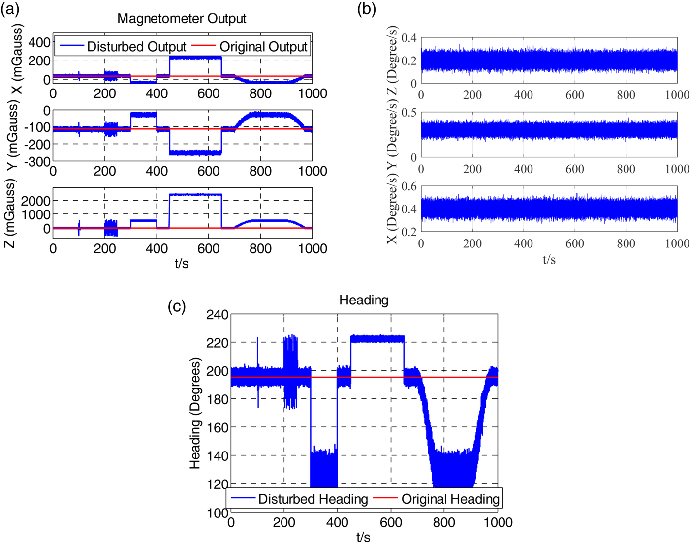
In data set A, the Disturbances (a), (b) and (c) appear separately and the arrangement in detail is as follows:
 $$\left\{\matrix{\hbox{Start}t=0 \hbox{seconds} \hfill \cr \hbox{A large noise disturbance }100<t< 105 \hbox{seconds} \hfill \cr \hbox{Continuous large noise disturbance }200<t< 250 \hbox{seconds} \hfill \cr \hbox{Step changed disturbance }300<t< 400 \hbox{seconds} \hfill \cr \hbox{Another step changed disturbance }450<t< 650 \hbox{seconds} \hfill \cr \hbox{Slow changed disturbance }700<t< 950 \hbox{seconds} \hfill \cr \hbox{End }t=1000 \hbox{seconds}\hfill \cr }\right.$$
Figures 5(a) and 5(b) show the disturbed magnetic field from the magnetometer and the gyroscope's output; the heading angle calculated by the disturbance magnetic field is expressed in Figure 5(c). It is obvious that the magnetic disturbance brings large errors to the magnetometer outputs and it also leads to a large heading error.
(a) Disturbed magnetometer output in data A, (b) Gyroscope data in data A, (c) Disturbed heading in data A.

4.2.2. Simulation data set B
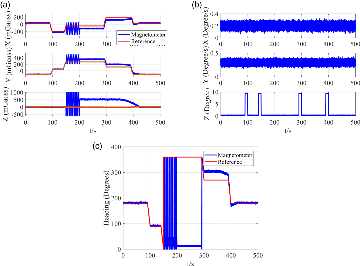
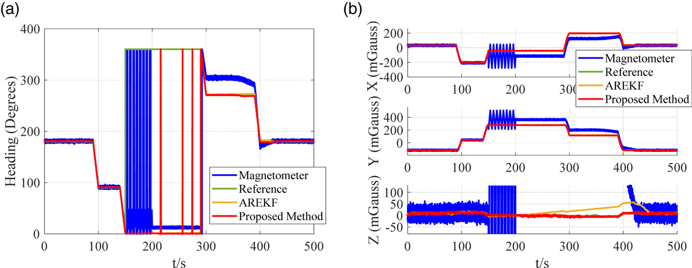
In data set B, complex disturbances occur and some changes in attitude have been added. Figure 6 presents the magnetometer's output, the gyroscope's output and the heading from the magnetometer.
(a) Disturbed magnetometer output, (b) The gyroscope output, (c) The disturbed heading in simulation data B.

4.3. Simulation Results
In this part the simulation results of reference algorithms and the proposed method will be shown.
4.3.1. Results of data set A
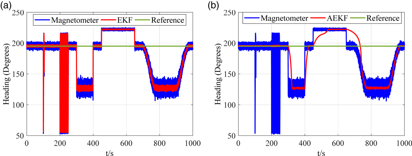
First, as heading can be calculated by the magnetometer, the heading results can represent the simulation results. Hence, in this section, the simulation results only show the heading results for convenience. Figure 7(a) shows the comparative heading results calculated by EKF and the direct output of the magnetometer. It can be seen that the heading of the EKF follows the magnetic disturbance. It can be concluded that EKF has anti-disturbance ability. In contrast, the AEKF can maintain stability when sudden disturbance appears in Figure 7(b). However, if the disturbance exists over a long time, it is difficult for the AEKF to overcome the disturbance.
The comparison heading results calculated by EKF in (a) and AEKF in (b).

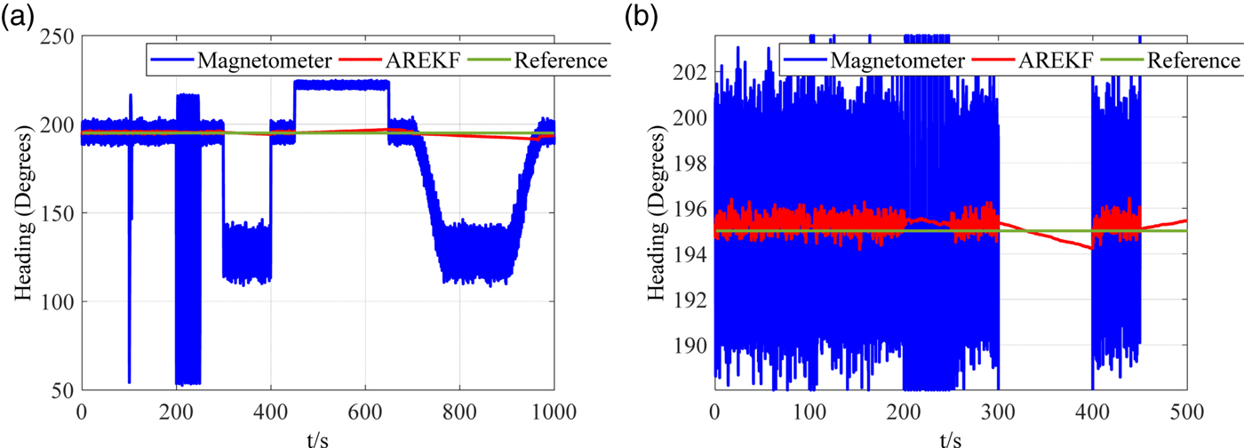
Figure 8(a) shows the results of AREKF and Figure 8(b) shows a partial enlargement. From Figure 8(a), it can be seen that AREKF can effectively overcome different disturbances whether sudden or long-term. However, from Figure 8(b), it can be seen that the heading angle still diverges slowly under long-term disturbance. This situation is possible in practice. For example, a MEMS integrated navigation system is installed on a car. When the car is close to a building and stops for some time, the magnetic disturbance will exist for a long time. The error of heading angle will slowly increase under such a disturbance.
The comparison heading results calculated by AREKF and magnetometer direct outputs in (a). (b) Shows a partial enlargement diagram.

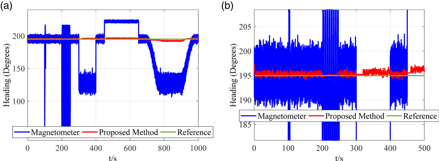
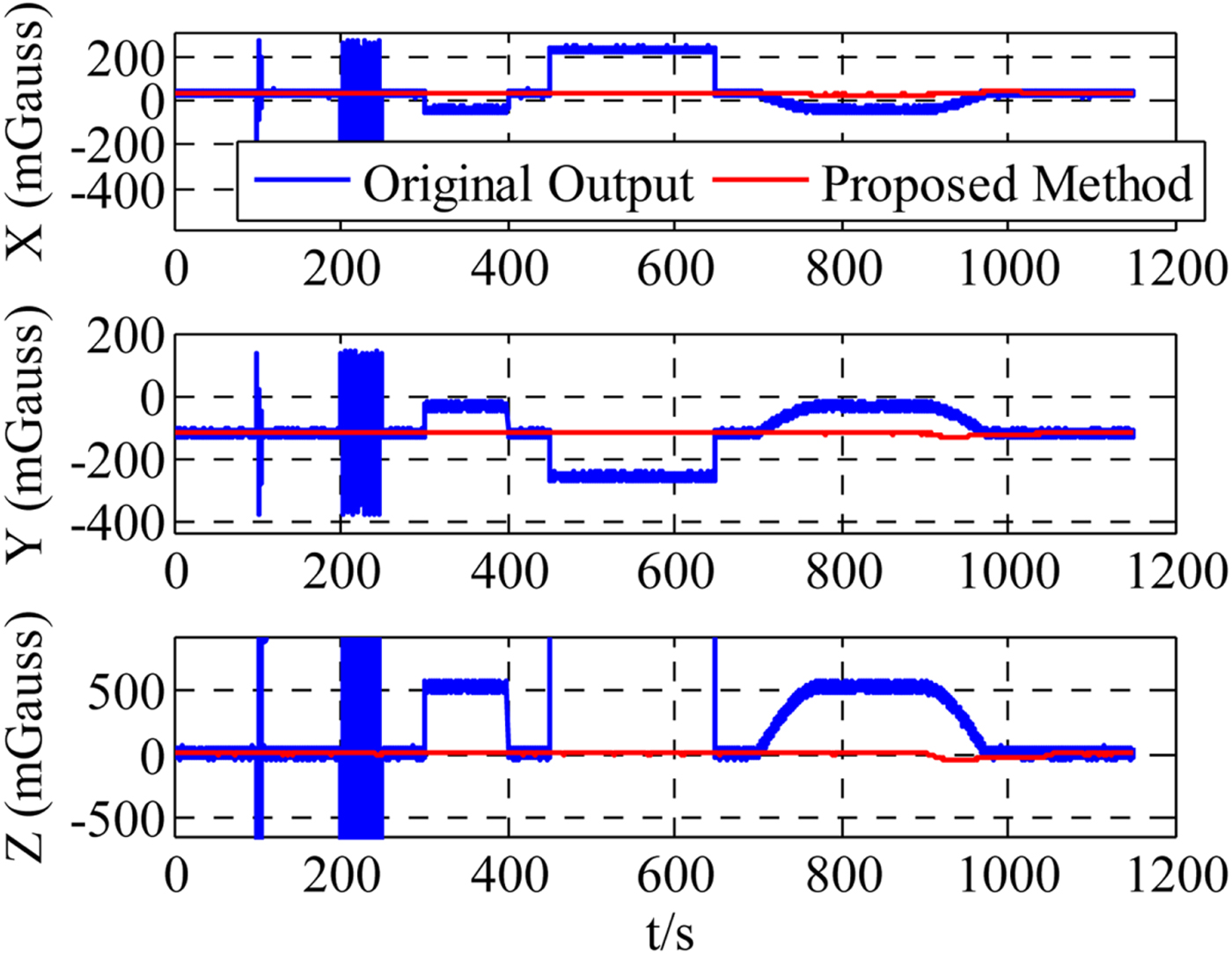
Aiming at the long-term disturbance situation, the proposed method calibrates the magnetometer under long-term disturbance. In Figure 9(a), the heading of the proposed method is shown and a partial enlargement diagram is displayed in Figure 9(b). From Figure 9(a), it can be seen that the proposed method can effectively overcome different disturbances. As can be seen from Figure 9(b), the magnetometer can be calibrated by using the data of the initial disturbance stage. After calibration, the magnetometer can compensate the heading error. This method greatly reduces the errors when a long-term disturbance occurs. Figure 10 shows the simulation results of the magnetometer's output with the proposed method.
The comparison heading results calculated by proposed method and magnetometer direct outputs in (a). (b) Shows a partial enlargement diagram.

The comparison diagram of magnetic fields from the proposed method and magnetometer direct outputs.

4.3.2. Results of data set B
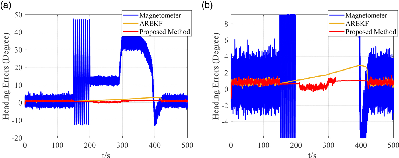
In this part, the simulation result using data set B is shown. Figure 11(a) and 11(b) show the heading results and magnetic fields results. Figure 12 shows the heading errors results. From Figure 11(a), it can be seen that the results of AREKF and proposed method can follow the reference when the attitude changes. From Figure 12, it can be seen that AREKF tends to diverge during long-term disturbances. In contrast, heading can be corrected by the magnetometer in the proposed method due to the magnetometer being recalibrated when a long-term stable disturbance is determined. Hence, the proposed method has a smaller error than the other compared methods.
(a) The heading results for simulation data B. (b) The magnetic fields results for data B.

(a) The heading errors results for simulation data B. (b) A partial enlargement diagram.

5. DRIVING TEST
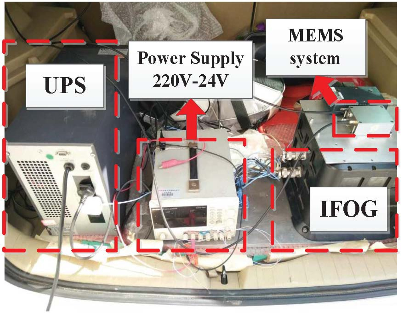
In this section, an actual driving test is used to verify the effect of the proposed method. A MEMS integrated system was installed in a car as shown in Figure 13. In Figure 13, a high precision inertial navigation system, an Interferometric Fibre Optical Gyroscope (IFOG), is taken as a reference. The MEMS system used was a ADIS16488 unit from the Analog Devices (AD) company and it is composed of a gyroscope, an accelerometer and a magnetometer. The detailed features are summarised in Table 3.
The MEMS system.

ADIS16488 and IFOG system features.

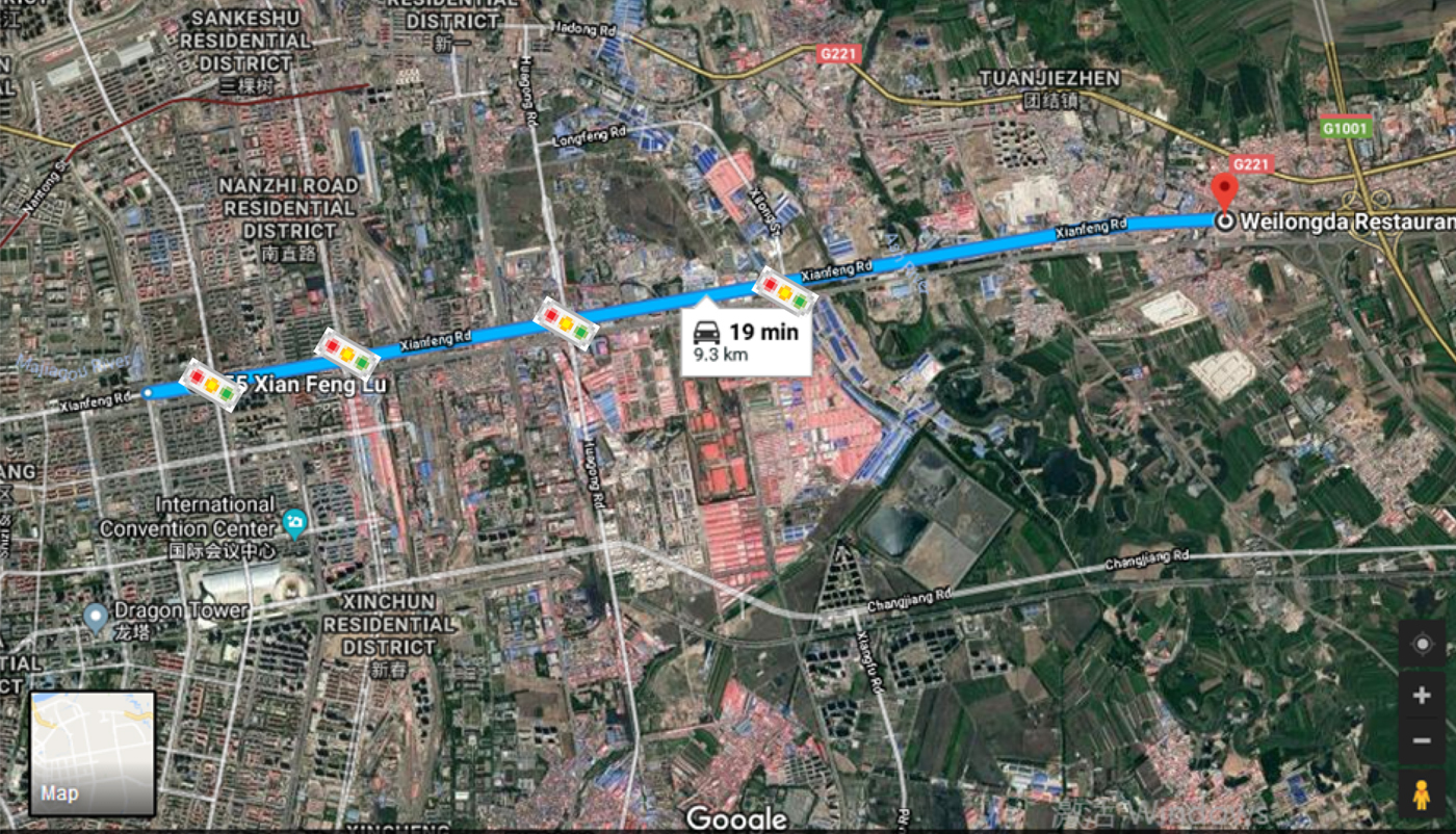
In order to clearly show the effect of disturbance, the driving route was selected as a straight road. The route is shown in Figure 14.
The driving test route.

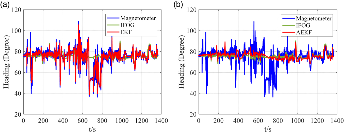
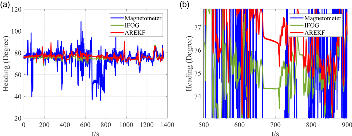
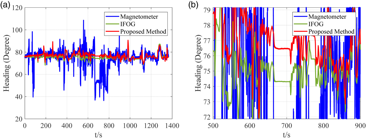
As can be seen from Figure 14, the route has four traffic lights and both sides of route are filled with buildings. The results of EKF, AEKF, AREKF and proposed method are compared.
From Figure 15, it is clearly seen that the EKF cannot filter any disturbances and AEKF can solve the large noise disturbance and sudden disturbance but is not successful at maintaining precision under step disturbances.
The comparison heading results calculated by EKF in (a) and AEKF in (b).

Figure 16 shows the result of AREKF and a partial enlargement graph. From Figure 16(a), it can be seen that AREKF can filter disturbances effectively. However, Figure 16(b) shows that the result of AREKF may diverge slowly when a disturbance remains for a long time.
The comparison heading results calculated by AREKF in (a) and a partial enlargement is shown in (b).

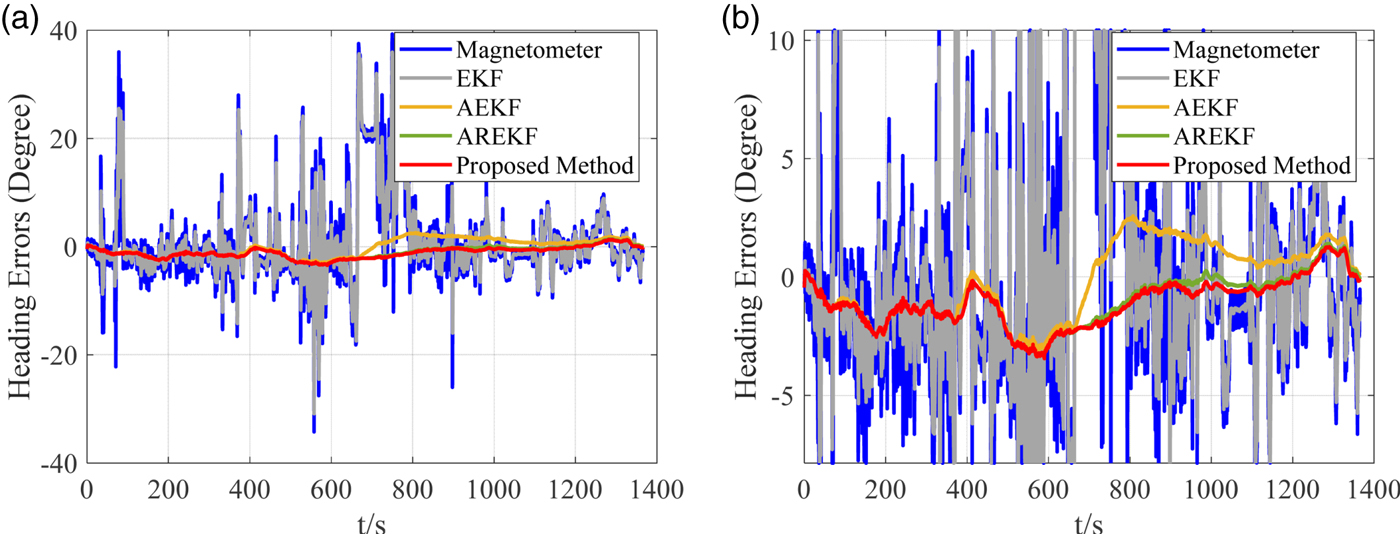
Compared with the above algorithms, the proposed method can filter disturbances as shown in Figure 17. When the long-term disturbance occurs, it also can remain stable as shown in Figure 17(b) because the proposed method considers magnetometer calibration. Figure 18 shows the heading errors of different algorithms and the detailed values are summarised in Table 4. The heading errors are the difference between the IFOG's heading and the calculated heading. From Figure 18 and Table 4, we can see that the proposed method and AREKF have similar results and their heading errors have significantly smaller peak to peak values than other algorithms during the different disturbances. Moreover, comparing Figure 16(b) and 17(b), it can be seen that the proposed method is more stable than AREKF when the stable disturbance is held longer. This result verifies that the heading errors are reduced from tens of degrees to a few degrees. It is evident that the proposed method has a better ability to face different kinds of disturbances.
The heading results by the proposed method in (a) and a partial enlargement in (b).

(a) The heading error results. (b) A partial enlargement diagram.

Heading Errors in the Driving Test.

6. CONCLUSION
This paper focuses on the problem that a magnetometer is disturbed by random magnetic disturbances during use, even if the magnetometer has been calibrated before leaving the factory. This problem not only leads to a large heading error, but also breaks the magnetometer's output model. Therefore, an adaptive anti-disturbance method for magnetometer and INS integration is proposed to solve this problem. This paper provides three contributions: (1) The random magnetic disturbances are accurately classified. (2) The update model of a magnetic field in the b-frame is deduced using angular velocity. (3) Aiming at the different kinds of disturbances, a cascaded filter with an anti-disturbance module and a magnetometer calibration module is proposed. By building simulation data sets A and B, the effects of existing methods and the proposed method were analysed under different kinds of disturbances, and the proposed method is better than the models tested for comparison. Finally, through an actual driving test, the proposed method was verified.
ACKNOWLEDGMENTS
This work is supported by the National Natural Science Foundation (61571148, 61871143), Fundamental Research for the Central University (HEUCFG201823, HEUCFP201836), Research and Development Project of Application Technology in Harbin (2017R-AQXJ095).