1 Introduction
To the fluid dynamicist, a fountain can be defined as a continuous and localised release of fluid for which buoyancy forces oppose momentum at the source. Following the initial rise, the flow collapses onto itself under gravity, with the classic picture of the flow comprising of a descending counterflow shrouding an ascending upflow. The many applications for fountains (see Hunt & Burridge (Reference Hunt and Burridge2015) for a review) have motivated their study in various configurations: axisymmetric (Turner Reference Turner1966) and planar (Zhang & Baddour Reference Zhang and Baddour1997), releases in stratified environments (Bloomfield & Kerr Reference Bloomfield and Kerr1998), non-Boussinesq (Mehaddi, Vauquelin & Candelier Reference Mehaddi, Vauquelin and Candelier2015), immiscible (Friedman et al. Reference Friedman, Vadakoot, Meyer and Carey2007), to name but a few. One class of fountains which has not yet been investigated is confined fountains, which arise when the flow is confined between two narrowly spaced plates. These plates serve to restrict the growth of the flow in the spanwise dimension, hence the flow develops primarily in the streamwise and cross-stream plane. Our focus in this paper is to investigate the dynamics of such confined fountains.
Confining shear flows in the spanwise direction is not a novelty. Confined jets, for instance, have long enjoyed considerable attention for their dispersive properties and applications to effluent discharge in shallow waters (Jirka Reference Jirka2001; Landel, Caulfield & Woods Reference Landel, Caulfield and Woods2012b
). More recently, confined plumes have come under investigation too (Rocco & Woods Reference Rocco and Woods2015). The literature commonly refers to these flows as ‘quasi-two-dimensional’, since their motion, being restricted in the spanwise direction, is (at the large scale) primarily in a plane. In these flows, instabilities rapidly induce a sinuous motion in the core (Chen & Jirka Reference Chen and Jirka1998). In turn, this motion prompts the development of large-scale counter-rotating eddies on alternate sides of the core which grow with downstream distance (
 $z$
) from the source and accentuate the jet’s (or plume’s) meandering (Landel, Caulfield & Woods Reference Landel, Caulfield and Woods2012a
). The onset of meandering marks the beginning of the far field and occurs around
 $z/W\gtrsim 10$
(Dracos, Giger & Jirka Reference Dracos, Giger and Jirka1992), with
 $W$
denoting the spanwise extent of the flow. Beyond this value, both the core structure and the surrounding eddies develop self-similarly; internal variables (such as the radius and velocity) retrieve the scaling of planar jets and plumes, respectively (Landel et al.
Reference Landel, Caulfield and Woods2012a
; Rocco & Woods Reference Rocco and Woods2015). To date, most studies have focused on the far field as being somewhat more relevant to environmental applications.
As a motivation for the current investigation, we ask what the corresponding behaviour is for confined fountains. Unlike jets and plumes, the rise of fountains is limited by their buoyancy, so that the scope for the interplay between large-scale eddies astride a meandering core is less clear. A far-field behaviour, therefore, may not always be reached, which suggests that a more nuanced view on the effects of confinement is appropriate for fountains. A priori, one might expect the dynamics to depend both on the degree of physical confinement and on the source Froude number
 $Fr_{0}$
(defined later);
 $Fr_{0}$
governing the final rise height of turbulent fountains (Turner Reference Turner1966; Hunt & Burridge Reference Hunt and Burridge2015). Other questions remain open too: for instance, do large-scale eddies persist in organising the motion, or are they shed from the driving core due to their density? It is the aim of this paper to provide an understanding of confined fountains by studying confined aqueous-saline releases in a series of experiments.
The remainder of the paper is structured as follows. In § 2, we describe the experimental method. Observations of the flow are reported in § 3, where we illustrate the different flow regimes in a series of snapshots. The thresholds for these regimes are first specified for a single confinement ratio
 $W/r_{0}$
in terms of source Froude numbers
 $Fr_{0}$
. Our quantitative analysis (§ 4) then reveals how to generalise the findings from § 3 to all confinement ratios examined herein by constructing a modified ‘confined’ Froude number. Rise heights, lateral excursions and characteristic frequencies are shown to collapse when scaled accordingly. Finally, we draw conclusions in § 5 and point to possible extensions of the current study.
2 Experimental procedure
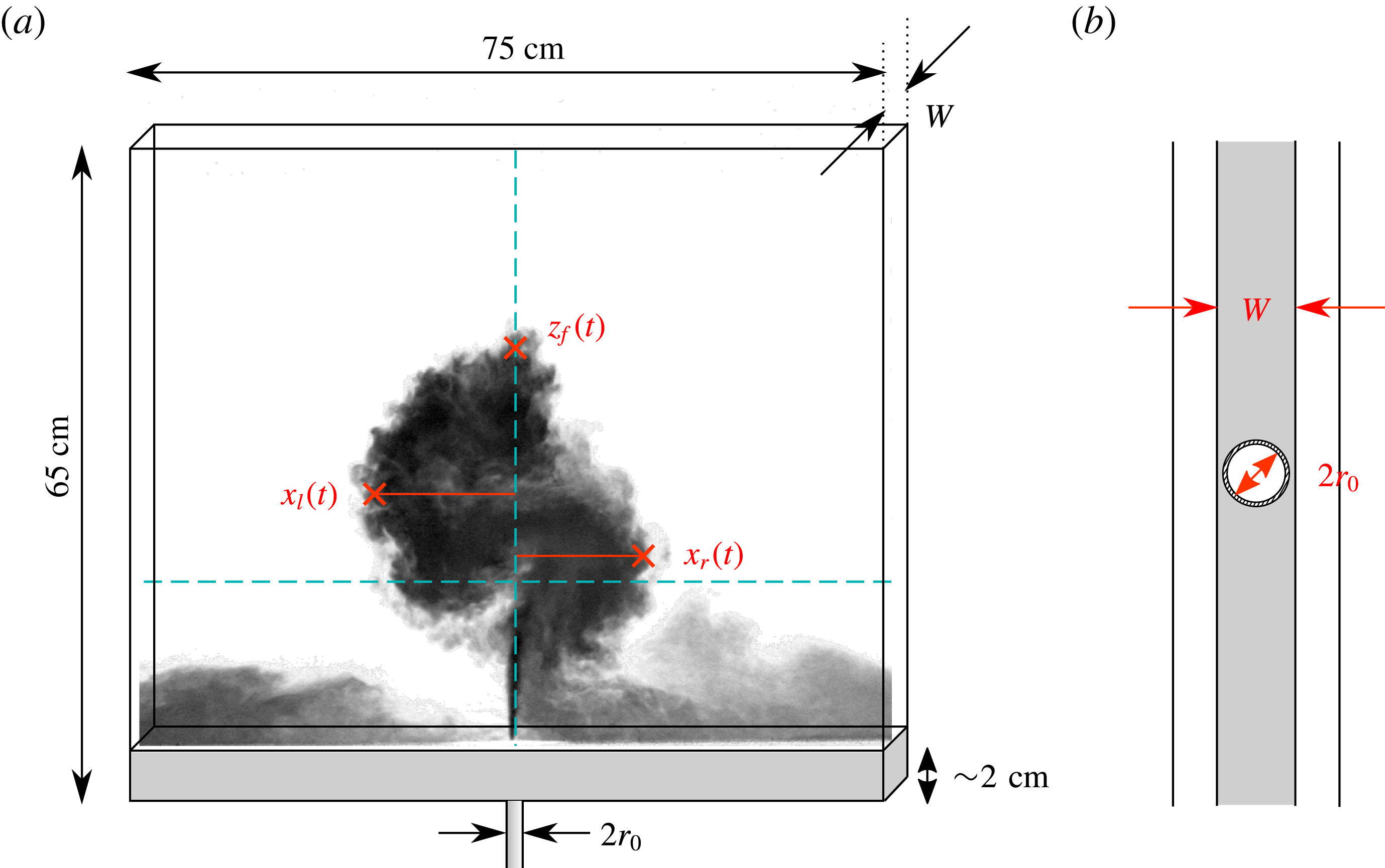
(a) Diagram of the experiment illustrating the two rectangular plates confining the fountain. A dyed saline fountain propagates through a narrow gap of width
 $W$
filled with fresh water and traces a typical S-shaped meander. The set-up is immersed in a large visualisation tank and open to the top, left and right sides, so that the fountain is free to entrain fluid from the ambient and to release the outflow sideways. The instantaneous (centreline) rise height
 $z_{f}(t)$
and the lateral extents of the fountain left
 $x_{l}(t)$
and right
 $x_{r}(t)$
are marked by crosses (see § 4). The vertical and horizontal dashed lines denote the centreline and half the time-averaged rise height
 $\overline{z}_{f}/2$
, respectively. (b) Top view of the nozzle and base used for set A,
 $W/r_{0}=2.7$
(table 1), representative of the fully confined case. In (b),
 $W=11.6~\text{mm}$
and
 $2\,r_{0}=8.6~\text{mm}$
.

Confined fountains were produced by continuously ejecting a dyed saline solution vertically upwards into a narrow gap from a round nozzle of radius
 $r_{0}$
. The gap, of width
 $W$
, was formed by attaching, with suction cups, a sheet of clear acrylic of dimensions
 $65\times 75~\text{cm}^{2}$
to the front face of a large, fresh-water-filled visualisation tank. The spacing
 $W$
could be accurately adjusted so to set
 $W$
within 0.5 mm using threaded rods mounted on the suction cups. The nozzle was installed flush in a horizontal PVC section (shaded grey in figure 1
a), of width
 $W$
, which was secured along the base of the acrylic sheet; thus, it prevented outflow through the base of the sheet, so that the fountain fluid left the gap sideways as a gravity current. Moreover, the PVC section helped minimise any potential warping and enforce the uniformity of the gap width across the sheet; spacers were positioned in the top corners to the same end. This experimental arrangement is depicted in figure 1(a). Note that the left, right and top sides of the gap are unobstructed, so that the fountain could freely entrain ambient fluid from the enclosing tank.

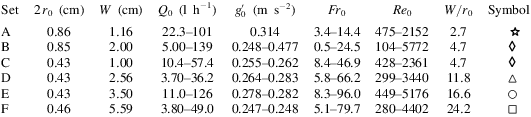
We conducted experiments at five different confinement ratios
 $W/r_{0}$
ranging from
 $2.7$
to
 $24.2$
. Additionally, one confinement ratio (
 $W/r_{0}=4.7$
) was achieved twice for different combinations of
 $W$
and
 $r_{0}$
, amounting to six sets of experiments. Of these sets, the set run at a confinement ratio of
 $W/r_{0}=2.7$
approaches the theoretical limit of complete confinement,
 $W/r_{0}=2$
. Material constraints such as the thickness of the nozzle wall prevented us from reaching lower values of
 $W/r_{0}$
. Nevertheless, the spacing between the inner walls of the nozzle and the confining side walls is narrow (
 $1.5$
mm either way for
 $2\,r_{0}=8.6~\text{mm}$
, figure 1
b), so that the experiments run at
 $W/r_{0}=2.7$
may be regarded as representative of the fully confined case.
Within each set, we set the separation
 $W$
on the acrylic sheet and installed a PVC section of appropriate width and nozzle radius before attaching our set-up to the inside of the visualisation tank. Great care was taken to ensure that the nozzle was aligned vertically. Then, within each set we varied the source Froude number
 $$\begin{eqnarray}\displaystyle Fr_{0}=\frac{w_{0}}{\sqrt{r_{0}\,g_{0}^{\prime }}}, & & \displaystyle\end{eqnarray}$$
where
 $w_{0}=Q_{0}/(\unicode[STIX]{x03C0}r_{0}^{2})$
denotes the cross-section-averaged source velocity and
 $g_{0}^{\prime }$
the source buoyancy, by increasing the volume flow rate
 $Q_{0}$
dispensed by an Ismatec ‘MCP-Z Process’ gear pump connected to the nozzle. This implies that the source Reynolds number
 $Re_{0}=w_{0}r_{0}/\unicode[STIX]{x1D708}_{0}$
(with
 $\unicode[STIX]{x1D708}_{0}=10^{-6}~\text{m}^{2}~\text{s}^{-1}$
the kinematic viscosity) was varied simultaneously; hence it is, in general, not possible to segregate
 $Re_{0}$
-effects in our results. In total,
 $278$
individual experiments were conducted over the ranges
 $0.5\leqslant Fr_{0}\leqslant 96$
and
 $104\leqslant Re_{0}\leqslant 5772$
. To our knowledge, this represents the highest
 $Fr_{0}$
at which round fountains have been investigated to date. For three of these experiments, the extent of the fountain occasionally exceeded that of the sheet of acrylic; this proved necessary to observe the qualitative behaviour of confined fountains at very high
 $Fr_{0}$
. Note, however, that their statistics are not included in our quantitative analysis. A summary of the experimental parameters are given in table 1.
The flow rates were measured on an Apollo ‘Lowflo’ flow meter during early experiments (sets B, C, D, F) and on an Altrato ‘Ultrasonic’ flow meter in later experiments (sets A, B, E). Whilst switching equipment during a campaign is unorthodox, in our case the switch was justified as the Altrato flow meter allowed us to log the trace of
 $Q_{0}(t)$
(see appendix A) and hence to exclude the possibility of the observed flow features being produced by irregularities in
 $Q_{0}$
. Experiments from set B were partially repeated to check for consistency between both devices, with good results (see § 4). Both flow meters have an accuracy of
 $\pm 1.0\,\%$
, which, together with a densitometer (Anton Paar ‘DMA 5000’) accurate to the fourth decimal, allowed
 $Fr_{0}$
to be reliably determined to within
 $3.9\,\%$
, at worst; the source buoyancy
 $g_{0}^{\prime }$
being measured as
 $g_{0}^{\prime }=(\unicode[STIX]{x1D70C}_{0}-\unicode[STIX]{x1D70C}_{a})/\unicode[STIX]{x1D70C}_{a}$
, with
 $\unicode[STIX]{x1D70C}_{0}$
and
 $\unicode[STIX]{x1D70C}_{a}$
designating the densities of the source solution and of the ambient, respectively.
For visualisation, the source solution was stained with methylene blue and backlit by an array of high-frequency fluorescent tubes. Recordings of the quasi-steady fountain, initiated after the initial transients had passed, were made on a JAI ‘CVM4
 $^{+}$
CM’ CCD camera at 12 or 24 frames per second. The recordings varied in duration, capturing well over
 $100$
buoyancy time scales
 $w_{0}/g_{0}^{\prime }$
in the majority of runs and never less than
 $40\,w_{0}/g_{0}^{\prime }$
. We then extracted flow statistics, such as those shown in figure 1, by tracking in time the edge of the fountain based on a luminosity (or density) threshold within an experimental error of
 $2.0\,\%$
. Given that a sharp interface was maintained at all times between the saline fountain and the fresh-water ambient, the data were not sensitive to the choice of threshold value. Edge detection algorithms which rely on luminosity gradients in the image, such as ‘Canny’ (Canny Reference Canny1986), were also implemented. The findings across both methods were consistent, differing only slightly in magnitude but not in scaling. For simplicity and consistency, we proceed to analyse the results obtained from thresholding the luminosity.
Finally, we note that the effects of wall friction will be neglected in this paper. Indeed, Dracos et al. (Reference Dracos, Giger and Jirka1992), who performed experiments of quasi-two-dimensional jets on an open water table, found that covering the water surface (i.e. introducing twice the friction) did not alter their measurements significantly. Likewise, Giger, Dracos & Jirka (Reference Giger, Dracos and Jirka1991) and Landel et al. (Reference Landel, Caulfield and Woods2012a
) estimated that the wall friction along their acrylic sheets resulted in a
 $10\,\%$
loss of momentum. This value is likely to act as an upper bound in fountains which, owing to their buoyancy, propagate less far: in Giger et al. (Reference Giger, Dracos and Jirka1991) and Landel et al. (Reference Landel, Caulfield and Woods2012a
), the
 $10\,\%$
loss was inferred over downstream distances from the source of
 $40W$
and
 $110W$
, respectively, whereas our fountains rise to
 $25W$
, at most (§ 4). In line with previous researchers, we therefore proceed on the premise that the effects of wall friction in our experiments are negligible.
3 Flow visualisation, observations and classification
Our observations lead us to propose a classification for confined fountain behaviour into four regimes (§§ 3.1–3.4). In order of increasing role of confinement, we refer to these regimes as:
(i) weakly confined regime;
(ii) asymmetric–stable regime;
(iii) transitional regime;
(iv) meandering (quasi-two-dimensional) regime.
The features characteristic of each are illustrated by means of time series of the fountain front
 $z_{f}(t)$
and snapshots of the flow taken from set B (
 $W/r_{0}=4.7$
). Each figure is accompanied by a video, available online, of the experiment from which the snapshots were extracted. We chose set B as a reference set to describe the regimes because the full range of regimes is observed only when the fountain transitions from being round at the source to being confined once it attaches to the walls. Fountains that are confined from the source (
 $W/r_{0}\rightarrow 2$
) exhibit only a subset of the regimes for reasons explained in § 3.5. As such, in the following the limits of each regime are stated in terms of
 $Fr_{0}$
-thresholds which pertain only to set B. We show how to generalise our findings to all confinement ratios considered herein in § 4.
3.1 Weakly confined regime,
 $Fr_{0}\lesssim 8$

Instantaneously, confined fountains produced for small
 $Fr_{0}$
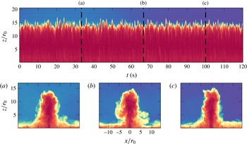
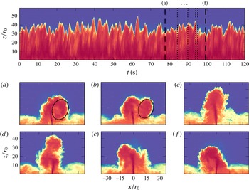
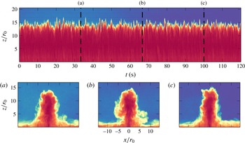
bear a strikingly similar appearance to their unconfined, axisymmetric counterparts. The resemblance is evident on comparing figure 2(a–c) to figure 2 in Burridge & Hunt (Reference Burridge and Hunt2012). The fountain consists of an upflow–counterflow double structure that is symmetric about the centreline and which fluctuates vertically about its time-averaged rise height. Visually, the fountain appears largely unaffected by the confinement.
A straightforward check allows us to confirm that the fountain is indeed in contact with the walls: were it unconfined, we expect the fountain top to attain an external radius of
 $b_{t}\approx 0.5\,r_{0}Fr_{0}$
(Burridge & Hunt Reference Burridge and Hunt2013; Hunt & Debugne Reference Hunt and Debugne2016). For the fountain shown in figure 2, produced at
 $Fr_{0}=5.4$
, this leads to
 $b_{t}>2.5\,r_{0}$
, i.e.
 $b_{t}>W/2$
and the fountain fills the gap. Moreover, it is clear that the induced radial inflow and the sideways fluctuations will prompt the fountain to cling to the walls sooner, though how much sooner is difficult to quantify. Crucially, the distance over which the fountain has clung is not sufficient to induce significant changes in its dynamics.
When the fountain is weak (
 $Fr_{0}\lesssim 2$
), such that the gap width is larger than but comparable to its external radius, the fountain cyclically attaches to the front and back wall as it precesses around the source. We report on this behaviour in appendix B. However, we do not include ‘weak’ confined fountains as a separate regime in our classification; the effects of confinement are indeed the same as in weakly confined fountains: the walls restrict the spanwise growth, but not sufficiently to induce two-dimensional effects.
Weakly confined fountains:
 $z_{f}(t)$
for
 $Fr_{0}=5.4$
and
 $W/r_{0}=4.7$
(see supplementary movie 1 available at https://doi.org/10.1017/jfm.2018.194). The dashed black lines in the main image correspond to the time series snapshots shown in panels (a–c). The bulk flow is unchanging (as illustrated by the sequence a–c) and visually indistinguishable from unconfined round fountains.
3.2 Asymmetric–stable regime,
$8\lesssim Fr_{0}\lesssim 12$

The effects of confinement become apparent beyond
 $Fr_{0}\sim 8$
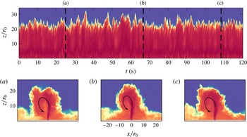
. Shortly after the initial (symmetric) rise-and-fall transient, any slight asymmetry or instability trips the counterflow so as to fall to the left or right of centreline. On the side to which the counterflow falls, a large recirculation region develops which extends from source to fountain top (figure 3). This recirculation region is maintained, forcing the fountain to arch over it. Most of the fountain fluid is therefore channelled along that arc and, in part, re-entrained into the upflowing core, as is highlighted by the curved arrow in figures 3(a–c). Patches that are not re-entrained disconnect (are shed) from the top of the recirculation region to form a (somewhat intermittent) gravity current on reaching the horizontal base. On the other side of the centreline, where the flow remains slender, smaller lobes are shed; their rate of shedding however appears more regular, hence the gravity current is more continuous on the slender side. Moreover, some fluid in the recirculation region crosses the centreline near the source and feeds into the replete gravity current.
Asymmetric–stable fountains:
 $z_{f}(t)$
for
 $Fr_{0}=8.9$
and
 $W/r_{0}=4.7$
(see supplementary movie 2). A sustained recirculation region forces the fountain to fold to one side (here, left of centreline in a–c) for the duration of the experiment, although some surges in rise height (‘spikes’) can momentarily perturb that arrangement. The curved arrow highlights the large-scale recirculation region.

The large recirculation region is to be likened to the large-scale eddies which typify confined jets and plumes. Thus, for
 $Fr_{0}\gtrsim 8$
we observe the first instance of (nascent) quasi-two-dimensional effects. A qualitative difference can also be noted from the time series in figure 3, where, by contrast with the weakly confined regime, departures about the mean are larger, and time scales associated with a given rise-and-fall event are longer. Strikingly, the fountain is unable to unbind from the recirculating region. Unlike jets and plumes which wind around eddies and propagate farther, for
 $Fr_{0}\sim 8$
the fountain is not sufficiently energetic to overcome the arched trajectory imposed by the recirculation region. Instead, on account of the arched trajectory, this implies that more dense fluid will be channelled toward and re-entrained into the folded side of the upflow, which in turn fuels the recirculation region, and so on.
The asymmetric configuration proved stable to relatively large disturbances. To illustrate this, we refer to the time series in figure 3 which showcases isolated disturbance events seen as ‘spikes’, in which a marked increase in rise height occurs (e.g. around
 $t=35~\text{s}$
). During these spikes, the fountain momentarily breaks loose from the recirculation region, rises rapidly upwards and then typically returns to its original asymmetric state. Only after
 $O(100)$
such spikes did the fountain eventually fold to the other side of centreline (as observed in
 $11$
out of
 $30$
experiments conducted in the asymmetric regime at
 $W/r_{0}=4.7$
), showing that the asymmetric state was robust. Changes in side were more frequent towards the higher end of the range
 $8\lesssim Fr_{0}\lesssim 12$
, when the flow, being more energetic at the source, overcomes the recirculation region more readily.
Transitional fountains:
 $z_{f}(t)$
for
 $Fr_{0}=14.0$
and
 $W/r_{0}=4.7$
(see supplementary movie 3). Instantaneous snapshots (a–f) illustrate the transition from one stable state (a) (folded left) to another (f) (folded right). The transitions are prompted by sporadic spikes in rise height (c), which appear as peaks in the time series.

3.3 Transitional regime,
$12\lesssim Fr_{0}\lesssim 16$

The fountain becomes increasingly unstable on further increasing the forcing at the source. While mostly retaining an asymmetric structure (figure 4 a), the flow now carries sufficient energy to sporadically unbind from the recirculation region (4 a,b, dotted outline). The latter is shed sideways, allowing the fountain to soar up as a near-symmetric jet (4 c). Subsequently, during collapse (4 d), instabilities prompt the flow to fold to either side of centreline and another recirculation region is rapidly re-established. The flow then locks into an asymmetric state until the next ‘spike’ (4 e,f). These spikes, which show as large peaks in time series 4, appear to have no one specific frequency associated with them; equally, intervals of lower rise heights (which mark periods of relatively stable, asymmetric flow) are also irregular in duration.
The principal difference between asymmetric–stable and transitional fountains is that, after being destabilised, transitional fountains show no preferential direction for folding. In addition, transitional fountains also display prolonged periods in which the flow flaps left and right several times before settling to one side. Both behaviours are indicative of a diminished influence of the recirculation region. As the fountain becomes increasingly forced, the recirculation region forms farther from the source and, as a consequence, becomes increasingly unable to sustain itself: whereas close to the source, the recirculation region is able to deflect the fountain towards it to fuel itself, when forming farther from the source it disconnects from the fountain and loses its bind on the central core (see § 3.4).
The transitional regime marks a range of Froude numbers for which the flow is neither stably asymmetric nor meandering (§ 3.4). As such, it shares features with both regimes, making a clear delineation difficult. Qualitative differences, such as repeated changes in flopping direction (compare supplementary movies 2 and 3), were used to classify the flow as either ‘asymmetric–stable’ or ‘transitional’. This led to the threshold between both regimes falling at
 $Fr_{0}\sim 12$
. We later allude to more rigorous approaches in § 4, which consist in comparing the average flow left and right of the centreline. However, the thresholds predicted by these approaches coincide with those inferred from straightforward observation.
3.4 Meandering (quasi-two-dimensional) regime,
$Fr_{0}\gtrsim 16$

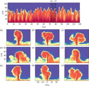
If one extrapolated observations of quasi-two-dimensional jets and plumes to flows with negative buoyancy, the ‘meandering’ (or quasi-two-dimensional) regime is what one would naturally anticipate. Large circulatory structures form, on a scale comparable to the rise height, at or near the peak of the fountain. After they disconnect from, and thus are no longer fed by, the upflow, the circulation of these structures rapidly dissipates, typically to cease rotating within a single revolution. Gravity then prompts them to fall around the upflow, randomly to the left and right. The upflow sinuously wraps around the descending structures; their presence deflects the upflowing core, soon prompting the growth of another eddy on the opposite side of the centreline to the previous structure. These cycles, of growth and decay on one side prompting growth and decay on the other side, repeat. Thus the fountain describes a sinuous or flapping motion, reminiscent of the meandering behaviour of quasi-two-dimensional jets and plumes. One such cycle is depicted in figure 5, with the growth and decay (a–d) of a ‘right’ eddy soon followed by the growth and decay of a ‘left’ eddy (e–i). Note how eddies ‘stack’ (figure 5 a,b), and hence how the behaviour is different from the flapping motion observed in planar fountains (Zhang & Baddour Reference Zhang and Baddour1997). Also discernible from 5(a–i) (as indeed from snapshots of all previous regimes) are small-scale eddies forming on the periphery of larger structures. Although the fountain has become quasi-two-dimensional at the large scale, the smaller scales which drive dissipation remain three-dimensional in nature.
It would be ill advised to regard the meandering regime as fundamentally different from previous regimes. Once circulatory structures form on a large scale and collapse around the fountain, their presence inclines the upflow away from them (figures 3 a, 4 a,f and 5 i). Simultaneously, as these structures collapse, dense fluid is re-entrained along one side of the upflow, creating a torque. If a structure forms sufficiently close to the source, this torque inclines the tip of the fountain, causing it to fuel the structure with lobes of fluid. The structure’s circulation, being fuelled, is maintained and the fountain locks into an asymmetric state. If, on the other hand, the structure forms farther from the source, it disconnects from the fountain core: its circulation rapidly dissipates and the structure collapses around the core, prompting the cycles of growth and decay on alternate sides of the fountain described in the paragraph above. Hence, the mechanism by which large-scale structures form is the same throughout all regimes; what varies, however, is the subsequent interplay between these structures and the fountain core.
Meandering fountains:
 $z_{f}(t)$
for
 $Fr_{0}=24.5$
and
 $W/r_{0}=4.7$
(see supplementary movie 4). Instantaneous snapshots (a–i), spaced one second apart, depict the growth and subsequent shedding of large-scale structures on alternating sides of the fountain that are typical of the meandering (‘forced’) regime.

3.5 Differences in behaviour with confinement ratio
The previous description of the four regimes applies to all values of
 $W/r_{0}$
explored in our experiments, albeit with different
 $Fr_{0}$
-thresholds (§ 4). However, some peculiarities of fountains at lower and higher
 $W/r_{0}$
are worth pointing out.
For strongly confined fountains (set
 $A$
,
 $W/r_{0}=2.7$
), the asymmetric–stable and transitional regimes are bypassed. Instead, they are replaced by a sustained flapping, with short-lived recirculation regions forming and shedding on alternate sides of the core. This behaviour is reminiscent of transitional fountains on the brink of meandering, although it persists throughout the transition from weakly confined to meandering. The flapping motion, as expected, then evolves into meandering at higher
 $Fr_{0}$
.
As in the asymmetric regime, the formation of large-scale structures (recirculation regions) signifies the onset of quasi-two-dimensional effects; unlike the asymmetric or the transitional regimes however, at
 $W/r_{0}=2.7$
these structures are not maintained. Notably, at this low confinement ratio we did not observe any significant amount of fluid crossing the centreline from one side to the other. At other confinement ratios, when a recirculation was maintained and dense fluid channelled towards the upflow, any excess fluid that could not be re-entrained crossed the centreline and fed into the opposite outflowing gravity current (§ 3.2). The narrowness of the gap at
 $W/r_{0}=2.7$
prevents this crossing, which might be instrumental in sustaining recirculation regions and hence, in sustaining a stable folded configuration.
Interestingly, this conclusion finds support in the contrasting observations made on line fountains by Baines, Turner & Campbell (Reference Baines, Turner and Campbell1990) and Zhang & Baddour (Reference Zhang and Baddour1997). Baines et al. noted that line fountains were mostly symmetrical about the centreline, but sporadically folded for prolonged periods of time. By contrast, in Zhang & Baddour, line fountains were reported to continually flap. An explanation for this discrepancy that is in line with our observations may be found in their source geometry. Whilst Zhang & Baddour dispensed fluid from a thin slot, Baines et al. approximated a line source with an array of closely spaced circular sources. Hence, close to the source their flow was three-dimensional. This arrangement permits a flow across the source from the folded recirculation region and, hypothetically, might allow the recirculation to be sustained. Conversely, such cross-flow is not possible with Zhang & Baddour’s source; thus, as in our strongly confined fountains, their line fountains flapped left and right.
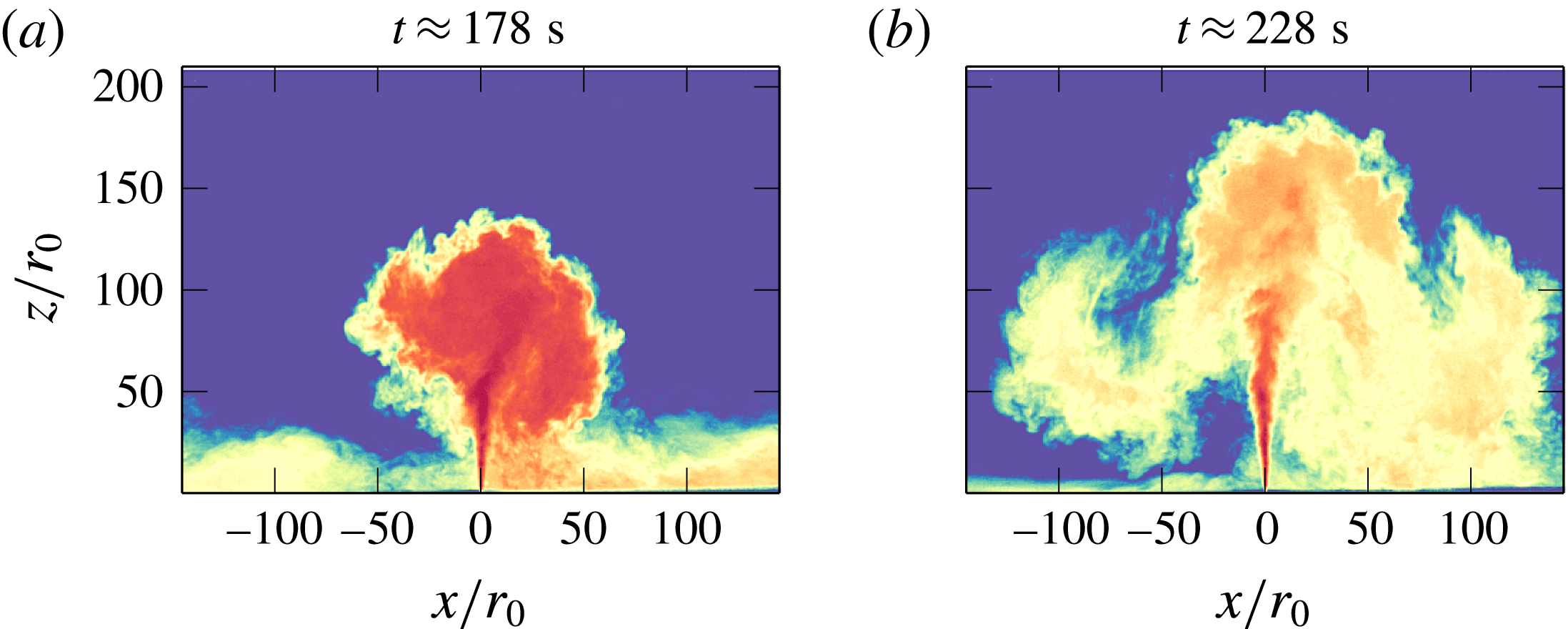
Illustration of a ‘burst’ event observed at
 $Fr_{0}=63.8$
and
 $W/r_{0}=11.8$
. The same colour map has been applied to (a) and (b), with dark red being indicative of high density. Whereas in (a) the fountain is dense and compact, in (b) it has spread and diluted significantly, leading to an increase in rise height of
 ${\sim}50\,r_{0}$
. Note that (a) and (b) are not correlated in time but have been chosen to maximise the contrast between the dense and the dilute configuration.

The next distinction needs to be made at moderate-to-high
 $W/r_{0}\,({\geqslant}11.8)$
, i.e. for weaker confinement. Fountains at these confinement ratios exhibited a greater range of dilution in our depth-averaged visualisations. Sporadically, the increased dilution led to ‘burst’ events, during which vast clouds of dilute fluid occupied a much larger space. This process is illustrated in figure 6, where we contrast two snapshots of the same run: the fountain is compact and dense in 6(a), whilst it is large and dilute in 6(b). The associated increase in rise height from (a) to (b) is approximately
 $50\,r_{0}\approx 4W$
.
The ‘bursts’ depicted in figure 6 occurred rarely and only for high
 $Fr_{0}$
, such that the fountain was meandering. Whilst we do not have the trace of
 $Q_{0}(t)$
for set D, which featured most bursts, we recorded
 $Q_{0}(t)$
at similar
 $Fr_{0}$
and found fluctuations of no more than
 $1\,\%$
(appendix A), which is insufficient to explain the observed increases in rise height.
It is relatively straightforward to reason why increased dilution leads to increased rise heights. Descending lobes of fluid that are more dilute and more spread out interact less strongly with the upflow, hence the fountain is free to rise vertically upwards. What is less clear is how the additional dilution is made possible. One explanation is that the fountain dilutes as a result of not completely filling the gap at all time. However, such behaviour was not observed in our experiments.
4 Experimental results
Having described the flow qualitatively in § 3, in this section we proceed to analyse the statistics extracted from the flow visualisation. Specifically, the flow visualisation allows us to track in time the outline of the fountain. Thus, we focus our analysis on three diagnostics (and on variables that can be constructed therewith):
 $z_{f}(t)$
, the rise height on the centreline;
 $x_{l}(t)$
, the farthest lateral excursions left of centreline; and
 $x_{r}(t)$
, the farthest lateral excursion right of centreline (figure 1). Note that we impose that
 $x_{l}(t)$
and
 $x_{r}(t)$
be at heights exceeding half the time-averaged rise height
 $\overline{z}_{f}/2$
(cf. the dashed horizontal line in figure 1), so as to avoid sampling the signal of outflowing gravity current.
Time-averaged centreline rise height
 $\overline{z}_{f}$
normalised by the source radius
 $r_{0}$
against
 $Fr_{0}$
for different values of
 $W/r_{0}$
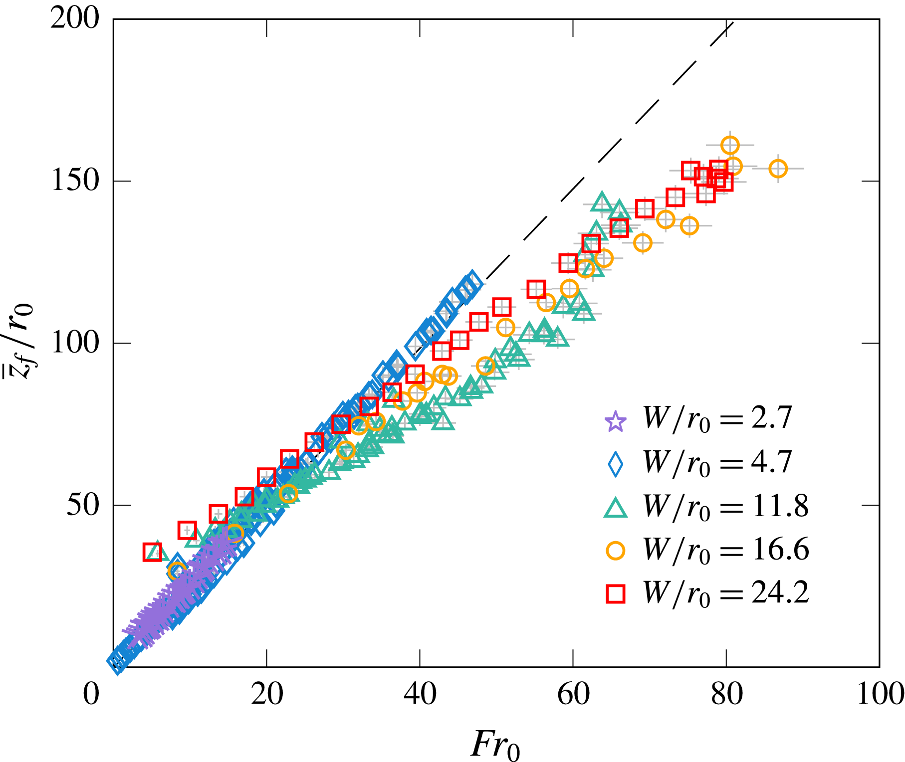
. The corresponding symbols for each confinement ratio are given in table 1 and repeated in the legend. The dashed line represents the rise height of unconfined round fountains,
 $\overline{z}_{f}=2.46\,r_{0}Fr_{0}$
(Hunt & Burridge Reference Hunt and Burridge2015). Error bars in light grey.

4.1 Rise heights and lateral excursions
We begin by inspecting the time-averaged rise height of the fountain front on the centreline,
 $\overline{z}_{f}$
. In figure 7, we apply the scaling for round unconfined fountains and plot
 $\overline{z}_{f}$
normalised by
 $r_{0}$
against the source Froude number
 $Fr_{0}$
. The plot encompasses all experimental sets. Two observations are immediately apparent: first, within each set the rise heights scale linearly on the jet length,
 $\overline{z}_{f}\propto r_{0}Fr_{0}$
, across all regimes; second, the gradient of that linear relation varies with
 $W/r_{0}$
. Indeed, the rise heights in sets B and C (

 $W/r_{0}=4.7$
) overlie, which confirms that the gradient is a function of
 $W/r_{0}$
rather than of
 $W$
or
 $r_{0}$
separately. Specifically, figure 7 suggests that increasing the gap width for a fixed Froude number causes
 $\overline{z}_{f}/r_{0}$
to decrease for confinement ratios
 $W/r_{0}\leqslant 11.8$
, but then to increase for
 $W/r_{0}\geqslant 16.6$
. This behaviour, which is difficult to rationalise, hints that
 $r_{0}$
is not an appropriate length scale. Note that for set D (▵), the last few experiments at the highest values of
 $Fr_{0}$
diverge from the linear scaling due to the ‘bursts’ reported in § 3.5.
Also plotted in figure 7 (dashed line) is the rise height for unconfined round fountains,
 $\overline{z}_{f}=2.46\,r_{0}Fr_{0}$
. We notice that the rise heights of relatively strongly confined fountains (low
 $W/r_{0}$
(


A notable preliminary result is nonetheless that
 $\overline{z}_{f}$
scales linearly on
 $Fr_{0}$
(the gradients for each set can be inferred from figure 8
a). As alluded to in § 1, the internal variables of quasi-two-dimensional jets and plumes recover the scaling of their planar counterparts for sufficiently large
 $z$
(Landel et al.
Reference Landel, Caulfield and Woods2012a
; Rocco & Woods Reference Rocco and Woods2015). Planar fountains rise as
 $\overline{z}_{f}\propto Fr_{0}^{4/3}$
(Baines et al.
Reference Baines, Turner and Campbell1990; Zhang & Baddour Reference Zhang and Baddour1997), in clear contrast with our measurements of confined fountains (figure 7). Of note is that in jets and plumes, variables such as the velocity are measured at, or near, the core of the flow, i.e. not at the periphery of the flow where eddies form. The core, which meanders between the eddies, maintains its coherence over height and is free to develop quasi-two-dimensionality. On the contrary, the upflowing core in fountains becomes progressively weaker with height as buoyancy depletes its momentum; near the top, the fountain is swayed by eddies to the extent that its motion becomes predominantly lateral. It is undeniable that eddies have a stronger and more disruptive influence on (or feedback with) fountains than in jets and plumes. The dynamics of confined fountains, being disrupted, becomes distinct from (free) planar fountains. It is therefore not surprising that their rise heights scale differently. Likewise, experiments on rectangular sources by Vinoth & Panigrahi (Reference Vinoth and Panigrahi2014) have shown that large source ratios are required at the source to attain the two-dimensional scaling. In our experiments, it is questionable whether the upflowing core, which remains slender (e.g. figure 5), departs sufficiently from being round to form a planar fountain. Again, therefore, we would expect
 $\overline{z}_{f}\propto Fr_{0}$
.
The fact that we observe the same qualitative behaviour for confined fountains at different values of
 $Fr_{0}$
and
 $W/r_{0}$
strongly suggests that there is a common scaling which applies to, and governs, confined fountains such as those studied herein (at least over the range of confinement ratios considered,
 $2.7\leqslant W/r_{0}\leqslant 24.2$
). We set out to identify this common scaling by collapsing the rise heights
 $\overline{z}_{f}$
across all confinement ratios.
First, we explore how the rise heights vary with the confinement ratio by extracting, for each value of
 $W/r_{0}$
, the gradients
 $k_{s}$
(where ‘
 $s$
’ reads ‘set’) of the linear relationship
 $\overline{z}_{f}/W=k_{s}Fr_{0}$
from figure 7. Here, we normalise the rise heights by
 $W$
rather than by
 $r_{0}$
since the fountain experiences the length scale
 $W$
as soon as it has expanded to reach the walls; suitably highly forced confined fountains are therefore expected to scale on
 $W$
. Since
 $W/r_{0}$
is constant within each set, the relationship
 $\overline{z}_{f}/r_{0}\propto Fr_{0}$
(figure 7) also implies that
 $\overline{z}_{f}/W$
scales linearly on
 $Fr_{0}$
. The gradients
 $k_{s}$
are plotted against the confinement ratio
 $W/r_{0}$
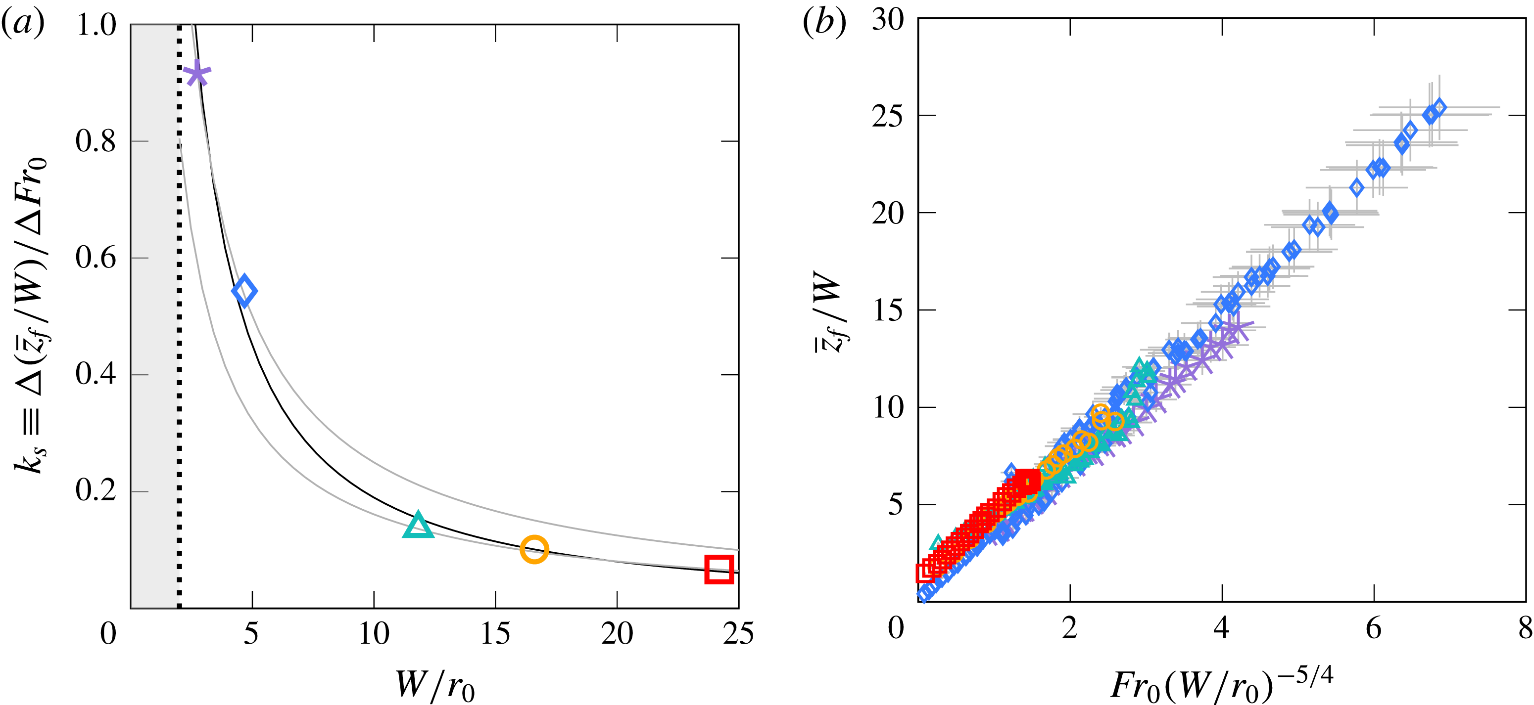
in figure 8(a). The rate of decrease of
 $k_{s}$
as a function of
 $W/r_{0}$
is notably steeper at low values of
 $W/r_{0}$
than at high values of
 $W/r_{0}$
, which implies that the rise heights are more sensitive to small changes in confinement when confinement is relatively strong (low
 $W/r_{0}$
) than when confinement is relatively weak (high
 $W/r_{0}$
). Most of the variation of
 $k_{s}$
with
 $W/r_{0}$
is therefore occurring at low values of
 $W/r_{0}$
. Of note is that the value of
 $k_{s}$
at
 $W/r_{0}=2.7$
(

 $13$
times greater than at
 $W/r_{0}=24.2$
(▫).
(a) Gradients
 $k_{s}\equiv \unicode[STIX]{x0394}(\overline{z}_{f}/W)/\unicode[STIX]{x0394}Fr_{0}$
, obtained from linear fits to the rise heights in figure 7, against
 $W/r_{0}$
. The black line represents the best fit (4.1) to the gradients as a function
 $W/r_{0}$
. In contrast to this best fit, grey lines highlight the discrepancy that ensues on adopting a simplified scaling for
 $k_{s}$
based on the assumption that, prior to attachment, the flow behaves like an unconfined fountain (appendix C). The shaded region demarks
 $W/r_{0}<2$
, which is not physical. (b) Time-averaged centreline rise height
 $\overline{z}_{f}$
normalised by
 $W$
against the confined Froude number
 $Fr_{c}\equiv Fr_{0}(W/r_{0})^{-5/4}$
(4.3). Error bars in light grey. Symbols as in table 1.

Next, attempting to derive the trend observed for
 $k_{s}$
in figure 8(a) on theoretical grounds is difficult in the absence of detailed measurements for the evolution of inner variables (e.g. the local velocity or buoyancy). We therefore opt to calculate, and adopt, a best fit through the gradients
 $k_{s}$
instead. The resulting power law, drawn in figure 8(a) as a black line, follows
 $$\begin{eqnarray}\displaystyle & \displaystyle k_{s}=3.32\left(\frac{W}{r_{0}}\right)^{-5/4}. & \displaystyle\end{eqnarray}$$
Equation (4.1) suggests that confined fountains reach a time-averaged rise height of
 $$\begin{eqnarray}\displaystyle & \displaystyle \overline{z}_{f}/W=3.32\,Fr_{0}\left(\frac{W}{r_{0}}\right)^{-5/4}+m_{s}, & \displaystyle\end{eqnarray}$$
where
 $m_{s}\sim 1$
denotes intercepts at
 $Fr_{0}=0$
. The normalised rise heights
 $\overline{z}_{f}/W$
are plotted against the suggested scaling
 $Fr_{0}(W/r_{0})^{-5/4}$
in figure 8(b). The collapse is excellent (with a mean coefficient of determination of
 $R^{2}=0.99$
), especially considering the range of parameters explored in this study. There remains a slight offset at the source,
 $m_{s}$
, which varies across sets, but typically
 $m_{s}\sim 1$
. Crucially, neither the scaling nor the pre-factor of the fit to
 $k_{s}$
(4.1) depend on
 $m_{s}$
, so long as
 $m_{s}$
is not a function of
 $Fr_{0}$
(as is indeed supported by the linear dependencies in figure 7, and by the collapse in figure 8
b).
Whilst our data do not extend beyond
 $W/r_{0}=24.2$
, and as such, we cannot verify the suitability of (4.2) at greater confinement ratios, the gentle slope of
 $k_{s}$
at higher values of
 $W/r_{0}$
(figure 8
a) implies that most of the variability of
 $k_{s}$
with
 $W/r_{0}$
has been captured by (4.1). Therefore, it seems likely that (4.2) should apply, at least in an approximate sense, at greater values of
 $W/r_{0}$
too. Equation (4.2) will not apply, however, in the limit of no confinement (
 $W/r_{0}\rightarrow \infty$
), where the rise heights scale as
 $\overline{z}_{f}/r_{0}=2.46\,Fr_{0}$
(Turner Reference Turner1966) and where accordingly, there can be no dependence on
 $W$
; see the discussion in § 5.
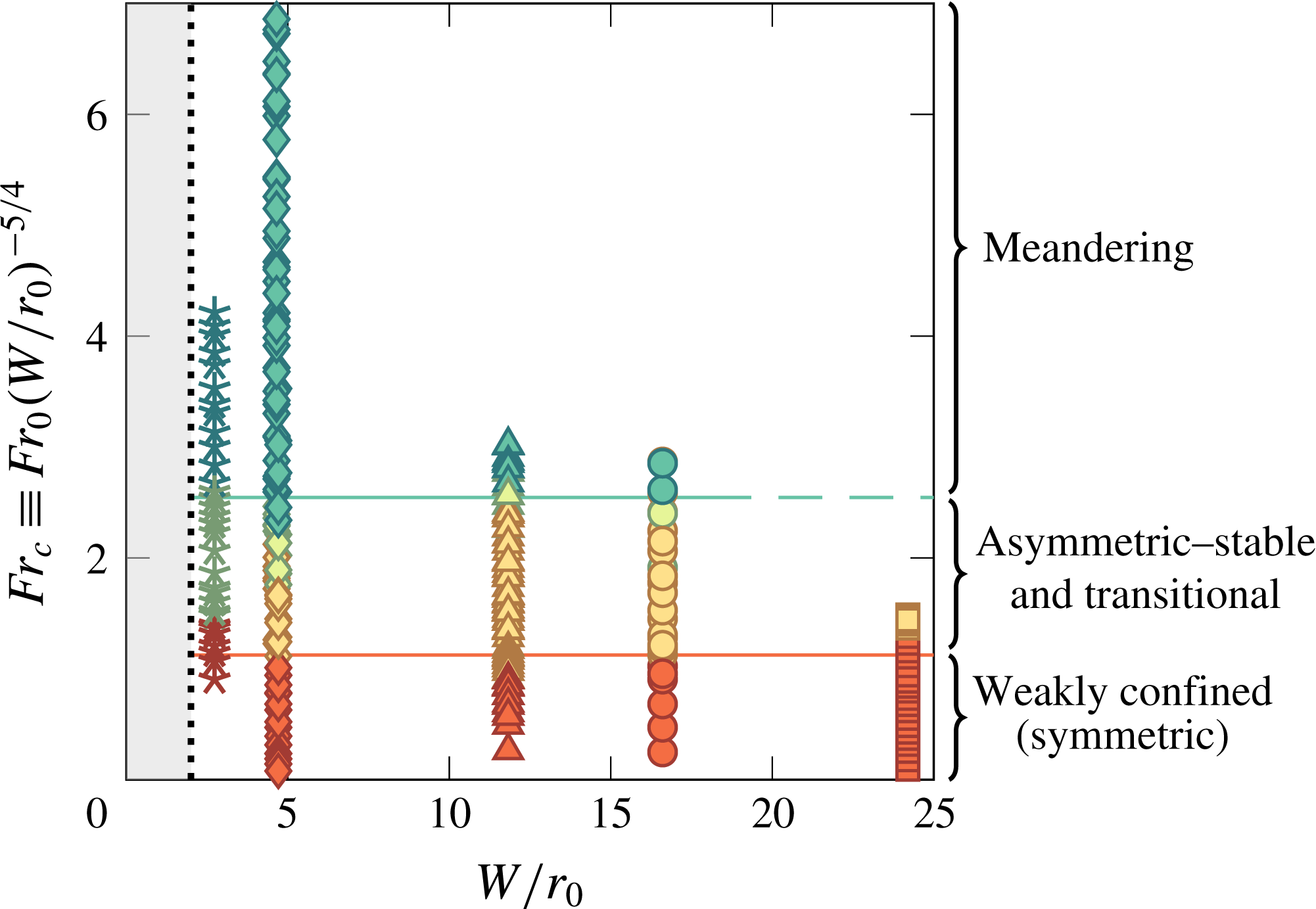
Regime diagram for the different flow regimes observed in § 3. Each experiment, run at a particular
 $\{Fr_{0},W/r_{0}\}$
, is colour-coded according to the observed flow behaviour of that experiment, with red (dark grey) representing
 $Fr_{c}=1.13+/-0.18$
, yellow (light grey) representing
 $Fr_{c}=1.86+/-$
0.33 and turquoise (mid-grey) representing
 $Fr_{c}=2.58+/-0.16$
. Horizontal lines, which represent average threshold values for
 $Fr_{c}$
(table 2), demarcate approximate boundaries for the symmetric–asymmetric transition (bottom line, red) and the transitional–meandering transition (top line, turquoise), respectively. The vertical dotted line denotes the limit of fully confined fountains,
 $W/r_{0}=2$
. The symbols, as in previous plots, represent different sets of experiments (table 1), although for the purpose of this plot their colour has been changed to refer to the flow regimes (see annotation).

The collapse of the rise height data in figure 8(b) across all values of confinement ratios tested herein provides convincing evidence that the scaling
 $Fr_{0}\,(W/r_{0})^{-5/4}$
encapsulates the dynamics of confined fountains. More evidence is provided later, e.g. in figures 9–11. Consequently, we define the ‘confined’ Froude number
 $$\begin{eqnarray}\displaystyle & \displaystyle Fr_{c}\equiv Fr_{0}\,(W/r_{0})^{-5/4} & \displaystyle\end{eqnarray}$$
as the governing parameter for confined fountains. In physical terms, identical values of
 $Fr_{c}$
can be achieved either on increasing the forcing
 $Fr_{0}$
for fixed
 $W/r_{0}$
, or on narrowing the dimensionless gap
 $W/r_{0}$
for fixed
 $Fr_{0}$
. Since
 $Fr_{0}$
is indicative of the height attained by the fountain, ‘confinement’ is therefore expressed in
 $Fr_{c}$
in terms of a ratio of the streamwise extent of the fountain to its spanwise extent (albeit not one to one).
If the confined Froude number
 $Fr_{c}$
is to encapsulate the effects of confinement, then bands of
 $Fr_{c}$
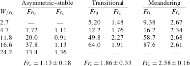
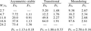
should coincide with the flow regimes observed in § 3. This notion is pursued in figure 9, where we colour-code every experiment according to their observed regime, and in table 2, where we cite the thresholds for the regimes in terms of
 $Fr_{0}$
for each set and calculate corresponding values of
 $Fr_{c}$
. In figure 9, horizontal lines (i.e. lines of constant
 $Fr_{c}$
) conclusively separate the colour-coded regimes. Likewise in table 2, we notice that
 $Fr_{c}$
takes a nominally constant value across all sets:
 $Fr_{c}\sim 1.1$
in the asymmetric regime and
 $Fr_{c}\sim 2.6$
in the meandering regime. Agreement in the transitional regime is poorer: by its very nature this regime marks a transition from one distinct behaviour to another, hence it is not surprising that transitional fountains are difficult to classify. Nevertheless, for threshold values of
 $Fr_{0}$
varying by a factor of
 $10$
, thresholds of
 $Fr_{c}$
vary by approximately 6 %–17 % only, a variation only slightly above our error margin. The overall ability of
 $Fr_{c}$
to delineate regimes, therefore, is good, reinforcing the suitability of the scaling (4.3).
Thresholds for the flow regimes (§ 3) for all confinement ratios considered in terms of source Froude number
 $Fr_{0}$
and confined Froude number
 $Fr_{c}$
(4.3). A blank entry (—) indicates that a regime was not observed in our experiments. The thresholds given correspond to the first value of
 $Fr_{0}$
for which the features characteristic of a particular regime first appeared. For a graphic representation of the onset of flow regimes as a function of
 $Fr_{c}$
and
 $W/r_{0}$
, the reader is referred to figure 9.
To readers familiar with work on unconfined fountains, the threshold values in table 2, and in general values of
 $Fr_{c}$
achieved in our experiments (
 $Fr_{c}\lesssim 7.0$
, figure 8
b), may appear low in magnitude. It is important to point out that, unlike unconfined fountains for which low values of
 $Fr_{0}$
do imply weak releases, in confined fountains low values of
 $Fr_{c}$
cannot be viewed as giving rise to momentum-poor fountains. The weakly confined fountain in figure 2, for instance, was formed at
 $Fr_{c}=0.78$
, yet it clearly retains the slender upflow–counterflow structure characteristic of highly forced (unconfined) releases. ‘Low’ values of
 $Fr_{c}$
(‘low’ relative to
 $Fr_{0}$
in unconfined fountains) should therefore not be mistaken for low levels of forcing. Weak confined fountains, such as shown in appendix B (where
 $Fr_{c}=0.08$
), probably occur at much lower values of
 $Fr_{c}$
and lie outside the scope of this paper.
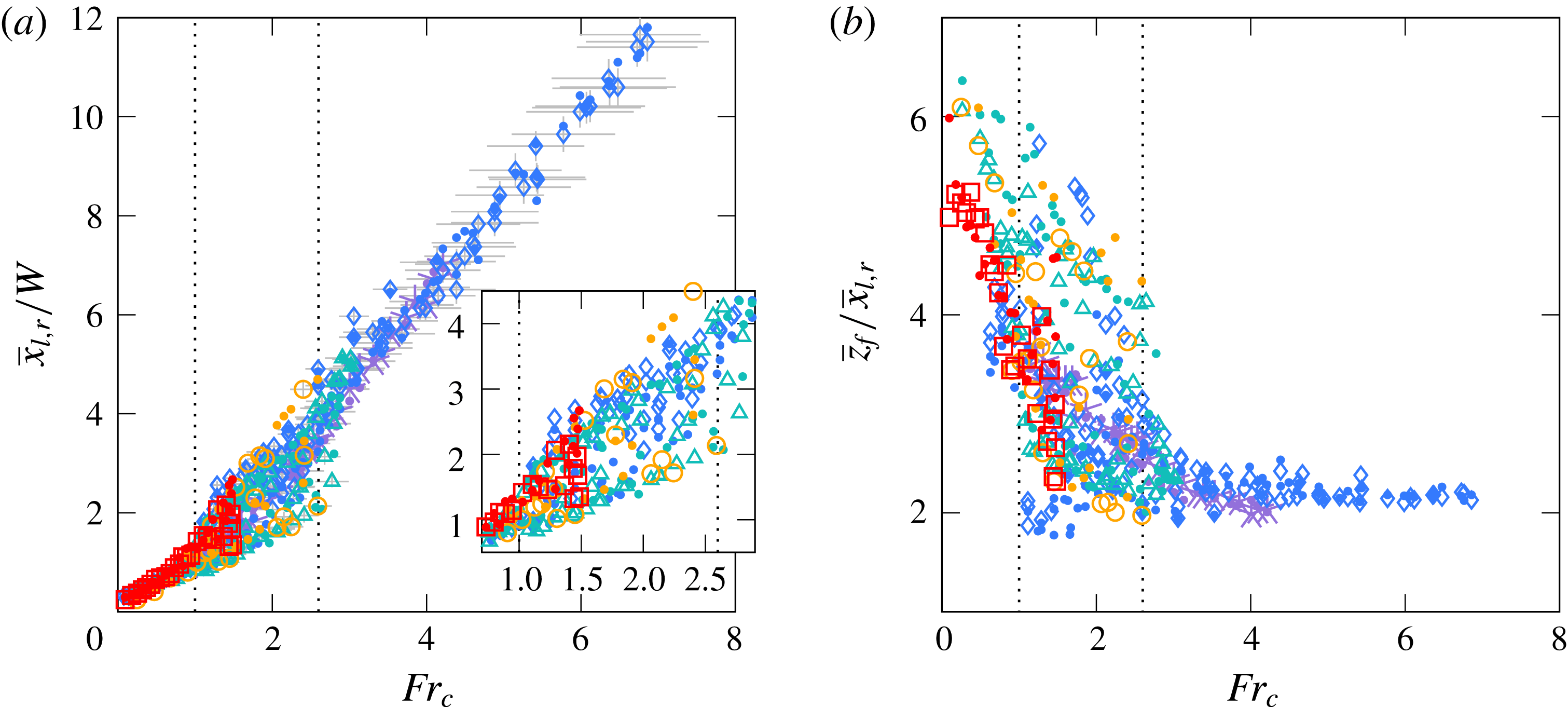
(a) Time-averaged lateral extent of the fountain left of centreline (
 $\overline{x}_{l}$
, various symbols) and right of centreline (
 $\overline{x}_{r}$
, dots) normalised by
 $W$
against the confined Froude number
 $Fr_{c}$
. For clarity, error bars (in light grey) are plotted for
 $\overline{x}_{l}/W$
only. The dotted lines delineate the limits for the asymmetric–stable and meandering regimes (table 2). The inset provides a zoomed view onto the interval
 $0.7\lesssim Fr_{c}\lesssim 2.9$
to highlight the formation of two distinct branches in the asymmetric–stable and transitional regimes. Set A is not plotted in the inset, because fountains in set A do not fold asymmetrically (and hence, their lateral extents to not splay). (b) Aspect ratio of the fountain: ratio of the rise height
 $\overline{z}_{f}$
to the lateral extent of the fountain
 $\overline{x}_{l,r}$
against
 $Fr_{c}$
for forced releases,
 $Fr_{0}\geqslant 3.0$
. Symbols and dotted lines as in (a).

Representative sizes for large-scale eddies, as inferred from the lateral fluctuations. (a) Time- and height-averaged eddy size
 $\overline{\unicode[STIX]{x1D706}}_{l,r}$
, and (b) time-averaged maximal eddy size
 $\unicode[STIX]{x1D6EC}_{l,r}$
, both normalised by
 $W$
, against
 $Fr_{c}$
. For clarity, error bars (in light grey) have been plotted for
 $\overline{\unicode[STIX]{x1D706}}_{l}$
and
 $\unicode[STIX]{x1D6EC}_{l}$
only. Symbols as in figure 10.

Next, we inspect a salient feature of confined flows, namely their considerable lateral excursions (as seen, for example, in figure 5
c). In order to analyse their extent, we consider separately the farthest points left (
 $x_{l}$
) and right (
 $x_{r}$
) of centreline which lie above
 $\overline{z}_{f}/2$
(figure 1). The minimal height of
 $\overline{z}_{f}/2$
is imposed only to avoid the lateral outflows and has little bearing on the results. Rather than tracking a specific point in the Lagrangian sense,
 $x_{l}(t)$
and
 $x_{r}(t)$
follow the extreme outer edge of the fountain regardless of the height at which this peak excursion occurs (so long as it exceeds
 $\overline{z}_{f}/2$
). Hence,
 $x_{l}(t)$
and
 $x_{r}(t)$
are susceptible to discontinuities or ‘jumps’. Whilst these discontinuities do not affect time averages, they will have to be taken into account later when estimating velocities based on the gradients of
 $x_{l}(t)$
and
 $x_{r}(t)$
.
The time-averaged lateral excursions
 $\overline{x}_{l}$
and
 $\overline{x}_{r}$
are normalised by the gap width
 $W$
and plotted against
 $Fr_{c}$
in figure 10(a). In order to not clutter the figure, the symbols (cf. table 1) were retained for the ‘left’ variables, but replaced by dots for the ‘right’ variables. As expected, the fountain grows laterally as
 $Fr_{c}$
increases. We note that left and right excursions generally overlap, but splay out in the asymmetric regime (
 $Fr_{c}\sim 1.1$
) where the fountain stably folds to one side (figure 3). The upper branch corresponds to the side on which the fountain has folded; the lower branch corresponds to the opposite side where, by comparison, the fountain is slender. The two branches then rejoin at the onset of the meandering regime (
 $Fr_{c}\gtrsim 2.6$
) and follow a linear scaling
 $\overline{x}_{l,r}\propto W\,Fr_{c}$
. A linear scaling is also observed in the weakly confined regime, albeit with a lower prefactor. These observations are reinforced in figure 10(b), where we plot the height-to-width aspect ratio of the fountain
 $\overline{z}_{f}/\overline{x}_{l,r}$
. For all values of confinement, the bulk structure of the fountain appears to be similar in
 $Fr_{c}$
. Moreover, we notice that the trends in figure 10(b) reflect the classification into regimes given in table 2: in the weakly confined regime, the aspect ratio is large (
 $\overline{z}_{f}/\overline{x}_{l,r}\sim 5{-}6$
) and similar to the aspect ratio of unconfined round fountains (Burridge & Hunt Reference Burridge and Hunt2013; Hunt & Debugne Reference Hunt and Debugne2016); then, as the asymmetric–stable regime is established, large circulatory structures begin to form, causing the aspect ratio to decrease; finally, in the meandering regime, the aspect ratio asymptotes to a constant value of approximately two, meaning that the fountain is as wide as it is high (adding
 $\overline{x}_{l}$
and
 $\overline{x}_{r}$
). Thus, figure 10(b) offers a new interpretation of the regimes in terms of the fountain’s height-to-width ratio.
4.2 Fluctuations
Having examined the time-averaged excursions
 $\overline{x}_{l,r}$
, we now turn to their fluctuating part. In particular, suitably chosen fluctuations about the mean excursion should be representative of the size of the large-scale eddies which typify confined flows.
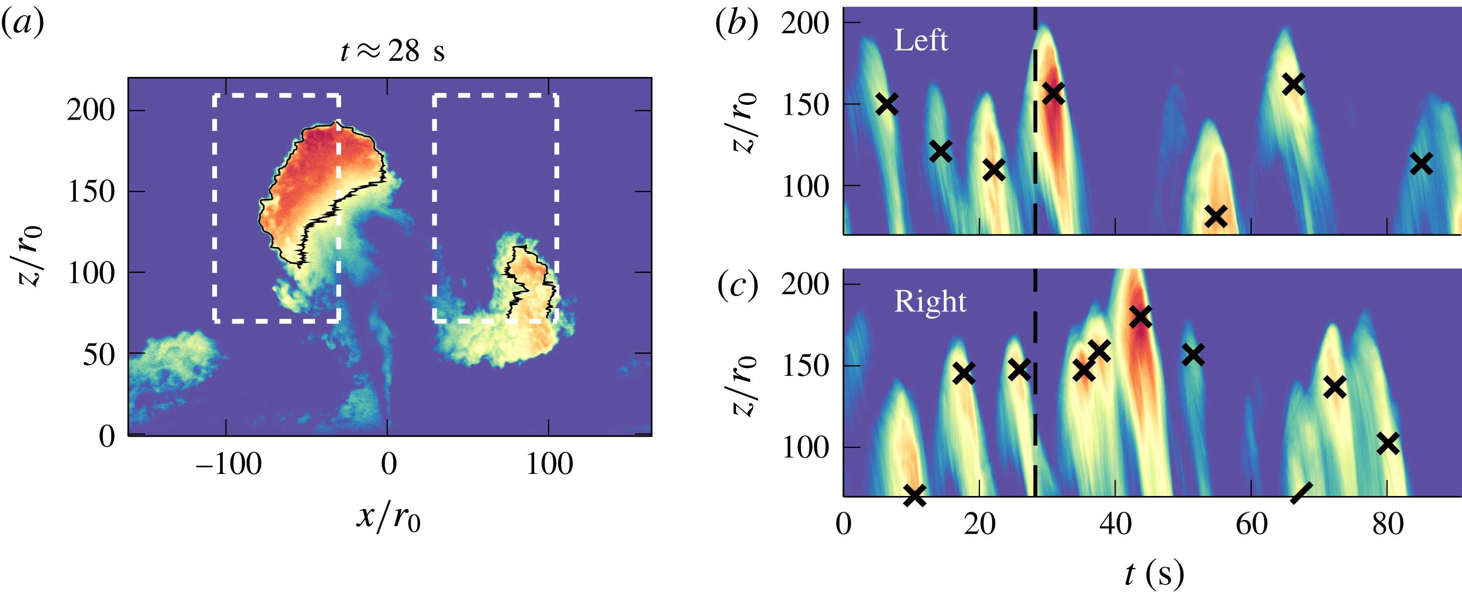
We first construct the ‘fluctuating’ part of our instantaneous snapshots by subtracting from each snapshot the experiment-averaged picture of the flow. In the resulting frames, the large-scale eddies are thereby made distinct from the fountain core and their outline can then be traced by applying a luminosity threshold (see the black lines in figure 12
a). For each (fluctuating) snapshot, we then record the lateral extent of eddies at every height to the left and right of centreline as
 $\unicode[STIX]{x1D706}_{l,r}(z,t)$
. Two key quantities are inferred: first, the average eddy size
 $\overline{\unicode[STIX]{x1D706}}_{l,r}$
, calculated by averaging in
 $z$
and
 $t$
; and second, the average size of large eddies
 $\unicode[STIX]{x1D6EC}_{l,r}$
, calculated by averaging in
 $t$
the instantaneous maxima in
 $z$
. As a remark, we note that many entries in
 $\unicode[STIX]{x1D706}_{l,r}(z,t)$
are zeroes, since eddies form intermittently and rarely at great heights. Therefore, in order to obtain representative eddy sizes, we average
 $\unicode[STIX]{x1D706}_{l,r}(z,t)$
over non-zero entries only.
Illustration of our ‘eddy counting’ approach for
 $W/r_{0}=11.8$
and
 $Fr_{0}=63.8$
. (a) An instantaneous snapshot from which the time-averaged luminosity has been subtracted. The black lines encircling eddies were used to calculate
 $\unicode[STIX]{x1D706}_{l,r}(z,t)$
(§ 4.2). The dashes outline the ‘windows’, left and right of the centreline, within which the luminosity is averaged (in
 $x$
) to produce the time series (b) and (c), respectively. In (b) and (c), crosses mark the detected peaks and the dashed line indicates the instant at which (a) was taken. The dashed line has just passed a peak in (c) (right window), and a remnant of the associated eddy is visible in (a). Similarly, the dashed line is approaching a peak in (b) (left window), and the nascent eddy can also be observed in (a). An animated version is available online (see supplementary movie 5).

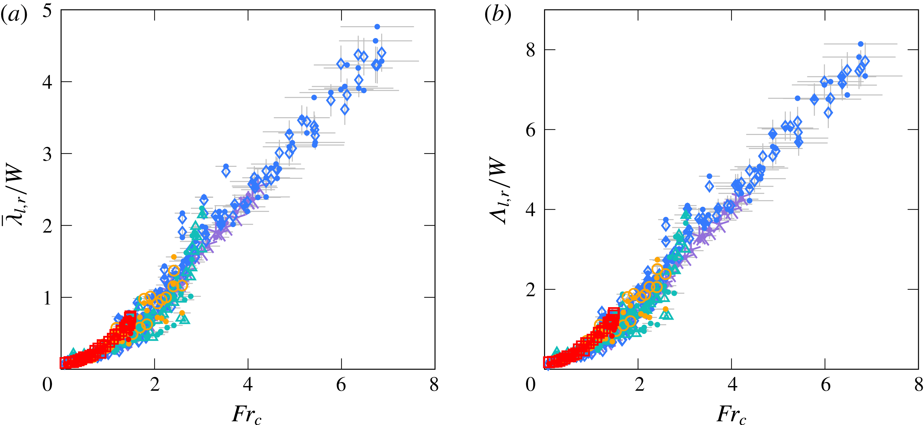
The results are shown in figure 11. Average (large-scale) eddies
 $\overline{\unicode[STIX]{x1D706}}_{l,r}$
and large (large-scale) eddies
 $\unicode[STIX]{x1D6EC}_{l,r}$
clearly follow the same trends, with
 $\unicode[STIX]{x1D6EC}_{l,r}$
being approximately a factor two greater. Similarly to the average excursions
 $\overline{x}_{l,r}$
in figure 10, three phases of growth can be distinguished: modest growth in the symmetric regime, followed by a phase of nonlinear growth in the asymmetric and transitional regimes as quasi-two-dimensional effects become prominent and finally linear (but accelerated) growth in the meandering regime. However, the measures
 $\overline{\unicode[STIX]{x1D706}}_{l,r}$
and
 $\unicode[STIX]{x1D6EC}_{l,r}$
are distinct from
 $\overline{x}_{l,r}$
in that they do not include the width of the upflow; thereby making them a more accurate measure of the scale of intermittent eddies. Landel et al. (Reference Landel, Caulfield and Woods2012a
), who studied the properties of large-scale eddies in quasi-two-dimensional jets, also noted a linear growth in the far field – here, that far field would correspond approximately to the meandering regime,
 $Fr_{c}\gtrsim 2.6$
. Over distances from the source comparable to the heights attained by our fountains, they reported eddy sizes between
 $4W$
and
 $4.5W$
, consistent in magnitude with our findings. Crucially, it is evident that the large-scale eddies occupy a significant proportion of the flow: ratios of
 $\overline{\unicode[STIX]{x1D706}}_{l,r}$
to
 $\overline{x}_{l,r}$
lie slightly above
 $1:2.5$
, whilst ratios of
 $\unicode[STIX]{x1D6EC}_{l,r}$
to
 $\overline{x}_{l,r}$
lie closer to
 $3:4$
. It is therefore not surprising that the dynamics of confined fountains is closely linked to the behaviour of large-scale eddies.
Various definitions for
 $\unicode[STIX]{x1D706}_{l,r}$
were considered before settling on the most intuitive, namely that associated with tracking the eddies’ outline. One alternative would have been to define average-sized fluctuations as twice the standard deviation
 $\unicode[STIX]{x1D70E}$
, or as a measure closely related. Landel et al. (Reference Landel, Caulfield and Woods2012a
), for instance, follow the centroid of eddies using particle image velocimetry measurements and infer typical eddy sizes as two standard deviations about the centroid’s location. Burridge & Hunt (Reference Burridge and Hunt2013) calculate the extent of vertical fluctuations in unconfined fountains as the difference between ‘peaks’ and ‘troughs’, which represent averages over time intervals when the rise height
 $z_{f}(t)$
is greater or lower than
 $\overline{z}_{f}\pm \unicode[STIX]{x1D70E}$
, respectively. Such definitions are meaningful when the underlying distribution is approximately symmetric; in that case, quantities above and below one standard deviation have a similar physical interpretation (e.g. ‘eddy present’ versus ‘eddy absent’). By contrast, the lateral fluctuations of confined fountains have a skewed distribution: there are more small-to-moderate lobes than there are large-scale eddies. Consequently it becomes less straightforward to interpret ‘one standard deviation’. We therefore resorted to the more natural approach of tracking the widths of eddies via
 $\unicode[STIX]{x1D706}_{l,r}(z,t)$
.
One drawback of this approach is that it cannot easily be extended to the vertical fluctuations in rise height. However, except in the weakly confined regime, the latter are not relevant dynamically. Only occasionally does a large eddy form at or near the centreline. Rather, the vertical fluctuations constitute a damped response to the left–right meandering of the fountain, which is dictated by the lateral fluctuations
 $\overline{\unicode[STIX]{x1D706}}_{l,r}$
. Hence, we do not further investigate the vertical fluctuations herein.
4.3 Frequencies
Based on figure 11 we established that the large-scale eddies grow larger with increasing
 $Fr_{c}$
. A natural continuation is to inspect the time scales over which these eddies form.
There are many techniques available to extract temporal information from a series of snapshots or signals. Decomposition methods, for instance, have successfully separated different oscillating modes in low-
 $Re_{0}$
fountains in Vinoth & Panigrahi (Reference Vinoth and Panigrahi2014). Burridge & Hunt (Reference Burridge and Hunt2013), in their study of fluctuations at the (unconfined) fountain top, performed Fourier transforms of the rise height signal
 $z_{f}(t)$
to identify dominant frequencies. Both methods are valid, but tend to require some tuning. In this section, we present a novel, intuitive approach in which eddies are ‘counted’ as they form. We demonstrate the robustness of this approach by comparing the resulting frequencies to those identified with Fourier transforms in appendix D.
Figure 12 depicts our ‘eddy counting’ approach. The main idea consists in identifying traces left by large-scale eddies in suitably constructed time series. Specifically, we wish to construct a
 $(z,t)$
time series by averaging the flow horizontally over a region where large structures typically form. By doing so, the large structures will appear in the time series as dense streaks separated by intervals of lighter ambient. These streaks are then counted, and their total is divided through the recording interval to calculate the formation frequency associated with large eddies.
Figure 12(a) shows an instantaneous snapshot from which the mean flow has been subtracted in order to increase the contrast between the intermittent eddies and the ever-present core. Then, as described above, the time series in figure 12(b,c) were obtained by averaging the flow horizontally over the ‘windows’ delimited by white dashed lines in figure 12(a). One clearly discerns streaks, which correspond to eddies forming and collapsing. These streaks were counted by identifying luminosity peaks in the time series. To ensure that our algorithm selected only large-scale eddies, we stipulated that the peaks exceed the median luminosity and had a width (at half-prominence) of at least half the median. These settings led to good detection properties while minimising omissions and double counting. The peaks thus detected are indicated by crosses in figures 12(b,c). We note very good agreement between separate bright streaks and detected peaks. In particular, for the time instant shown in figure 12(a) (marked as a dashed line in 12
b,c), our algorithm is about to successfully identify the formation of an eddy to the left of the centreline. Our results were not sensitive to the size of the windows, provided they were sufficiently large so as to enclose the majority of eddies. We opted for windows spanning
 $([-1.8\,\overline{x}_{l},-0.5\,\overline{x}_{l}],[0.5\,\overline{z}_{f},1.5\,\overline{z}_{f}])$
and
 $([0.5\,\overline{x}_{r},1.8\,\overline{x}_{r}],[0.5\,\overline{z}_{f},1.5\,\overline{z}_{f}])$
left and right, respectively.
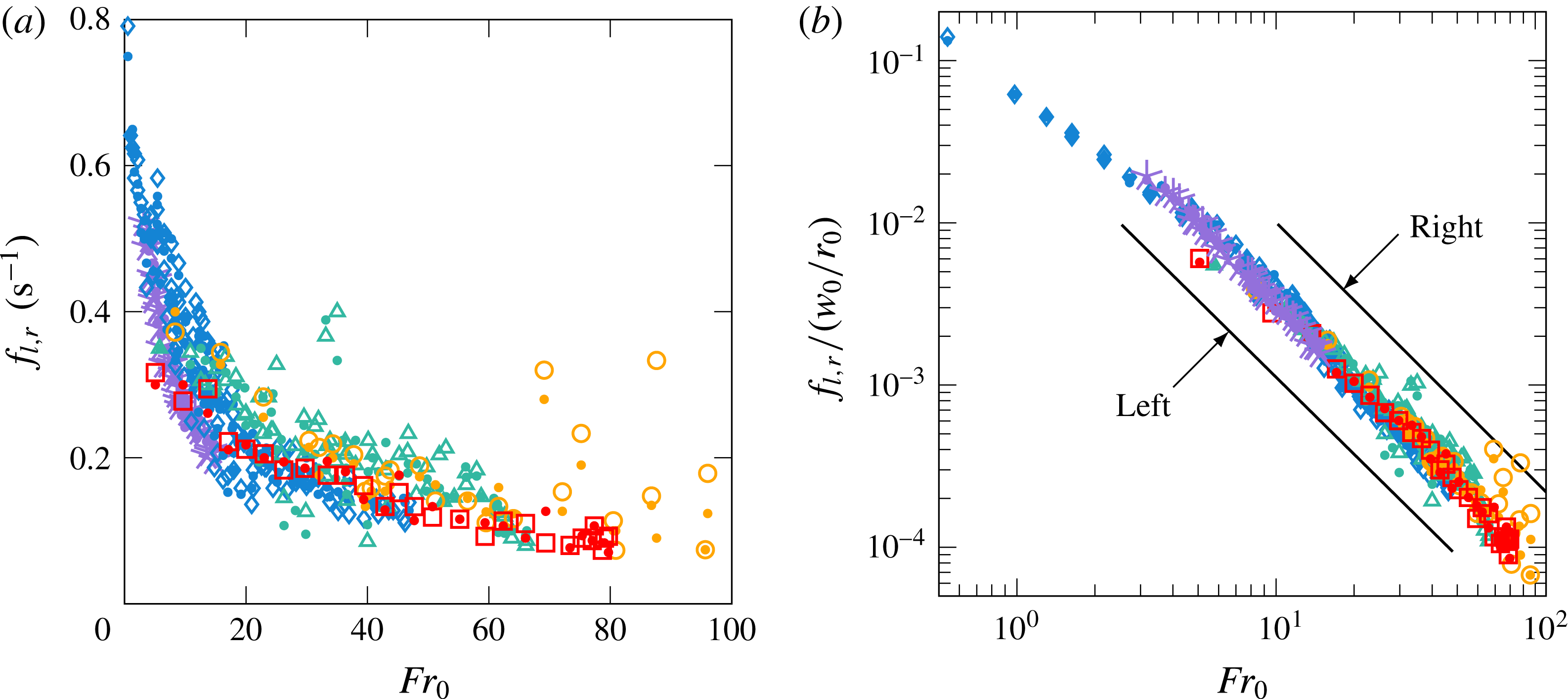
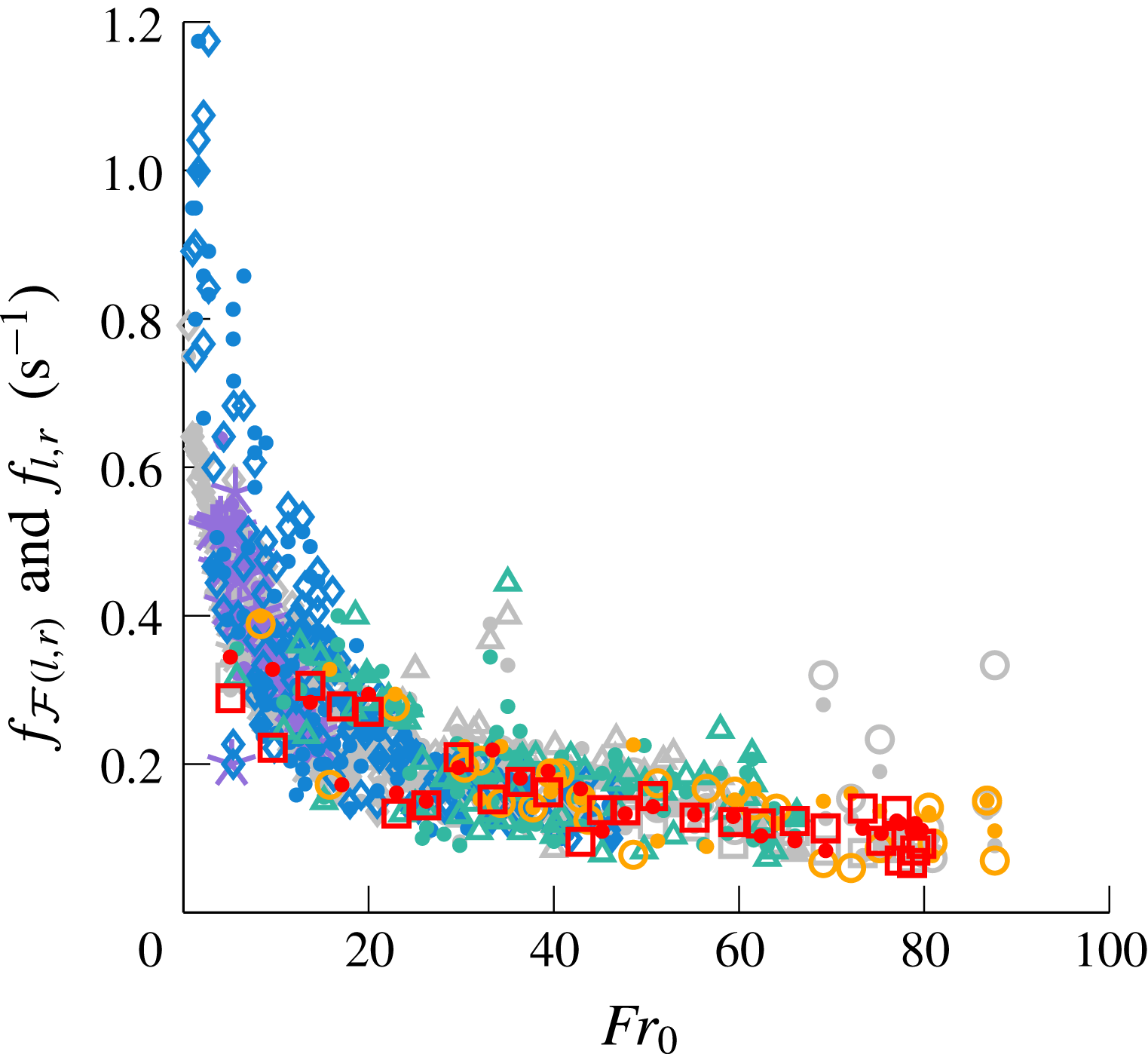
Formation frequencies
 $f_{l,r}$
of large-scale eddies to the left and right of centreline identified by our ‘eddy counting’ approach: (a) in dimensional form and (b) normalised by the source frequency
 $w_{0}/r_{0}$
. In (b), solid lines denote best fits for
 $f_{l}$
and
 $f_{r}$
over
 $Fr_{0}\geqslant 3$
(shifted for ease of reading). Symbols as in figure 10.

The formation frequencies
 $f_{l,r}$
are plotted against
 $Fr_{0}$
in dimensional form in figure 13(a). The error in
 $f_{l,r}$
was estimated as
 $\pm 2/\unicode[STIX]{x0394}T$
, where
 $\unicode[STIX]{x0394}T$
is the recording interval. The resulting error bars were mostly smaller than the symbol size and are omitted for clarity. The formation frequencies decrease as
 $Fr_{0}$
is increased, consistent with the notion that eddies grow larger and more persistent with
 $Fr_{0}$
(figure 11). At moderate
 $Fr_{0}$
, the ‘eddy counting’ approach predicts formation frequencies in the range
 $0.1{-}0.2~\text{s}^{-1}$
, i.e. one eddy being formed (left or right) every
 $2.5{-}5~\text{s}$
, which agrees well with our observations. We notice that, although there is some variation across the experimental sets, the formation frequencies generally lie close together, which suggests that the gap width
 $W$
has little influence on the formation of eddies. This is confirmed in figure 13(b), where we normalise
 $f_{l,r}$
by the source frequency
 $w_{0}/r_{0}$
. All sets fall onto one line, regardless of regime or confinement ratio. Lines of best fit yield the relations
 $$\begin{eqnarray}\displaystyle \frac{f_{l}}{w_{0}/r_{0}}=0.126\,Fr_{0}^{-1.58}\quad \text{and}\quad \frac{f_{r}}{w_{0}/r_{0}}=0.131\,Fr_{0}^{-1.60}, & & \displaystyle\end{eqnarray}$$
with coefficients of determination
 $R^{2}=0.97$
and
 $0.98$
, respectively. A similar scaling is retrieved when extracting
 $f_{l,r}$
via Fourier transforms of
 $x_{l,r}(t)$
(appendix D), hence (4.4) is not unique to our approach. Moreover, our attempts to include
 $W/r_{0}$
in the frequencies inevitably separate the data points into their respective sets, unless the scaling is chosen such that
 $(W/r_{0})^{-5/4}$
cancels out (i.e.
 $f_{l,r}\,(W/r_{0})^{2}\propto (w_{0}/r_{0})\,Fr_{c}^{-1.60}$
). We conclude that the gap width does not affect the formation frequencies.
The absence of a dependence on
 $W$
from (4.4) is counter-intuitive and not well understood. Based on our observations, the quasi-steady flapping appears to stem from the interplay between the large-scale eddies and the fountain core (see § 3.4), rather than, say, from instabilities propagating from the source. Following this reasoning, the formation of eddies, being a large-scale process, should accordingly scale on
 $W$
. An argument, however, which supports the absence of
 $W$
in the frequency scalings centres on the volume of large-scale eddies
 $V_{e}$
, which follows
 $V_{e}\sim W\overline{\unicode[STIX]{x1D706}}_{l,r}^{2}\propto r_{0}^{3}Fr_{0}^{2}$
(from
 $\overline{\unicode[STIX]{x1D706}}_{l,r}\propto WFr_{c}$
, figure 11). Thus,
 $V_{e}$
is independent of
 $W$
. Although this still poses constraints on the volume flux supplying the eddies
 $Q_{e}$
, it is at least conceivable that
 $f_{l,r}\sim Q_{e}/V_{e}$
is independent of
 $W$
. Likewise, it is worth recalling that, within each set, the rise height
 $\overline{z}_{f}\propto r_{0}Fr_{0}$
; the gap width entering only when a common scaling is sought across the sets. It therefore seems plausible that
 $W$
indeed cancels out in (4.4).
Finally, it is traditional for studies on confined flows to recast the formation frequencies of large-scale eddies into Strouhal numbers. Herein, we define the lateral Strouhal numbers
 $$\begin{eqnarray}\displaystyle St_{l,r}\equiv \frac{f_{l,r}}{\hat{u} _{l,r}/\overline{\unicode[STIX]{x1D706}}_{l,r}}, & & \displaystyle\end{eqnarray}$$
where
 $\hat{u} _{l,r}$
represents the characteristic velocity of large-scale eddies, defined later. Equation (4.5) is equivalent to rescaling the formation frequencies
 $f_{l,r}$
on length and velocity scales that pertain to the large-scale eddies themselves, rather than to the fountain. In quasi-two-dimensional jets, Landel et al. (Reference Landel, Caulfield and Woods2012a
) found Strouhal numbers ranging between
 $0.07$
and
 $0.25$
, approximately, at downstream distances of
 $20W$
to
 $60W$
. Specifically, the Strouhal number associated with a single eddy increased with downstream distance until merger with another eddy, at which point it consistently dropped to
 $0.07$
. These observations echo those of Dracos et al. (Reference Dracos, Giger and Jirka1992). Rocco & Woods (Reference Rocco and Woods2015) reported that the core meandered at an average Strouhal number of
 $0.16$
in quasi-two-dimensional plumes, which should broadly reflect the Strouhal numbers of lateral eddies.
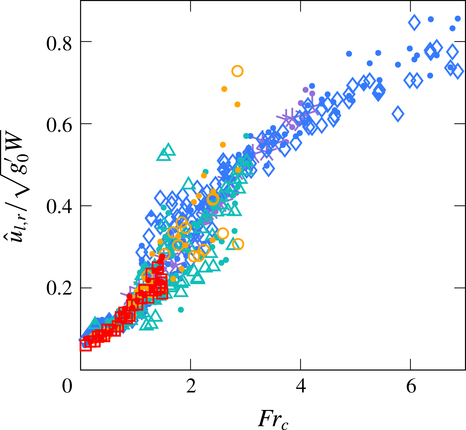
Unfortunately, we do not have direct measurements of the velocities. Nevertheless, we may gain an estimate of the velocities representative of large-scale eddies by differentiating in time the position of the eddies’ edge,
 $x_{l,r}(t)$
. The characteristic velocities
 $\hat{u} _{l,r}$
are then calculated as the root mean square (r.m.s.) of
 $\text{d}x_{l,r}/\text{d}t$
. Some precaution is necessary given that
 $x_{l,r}(t)$
is not a smooth or continuous signal (see § 4.1). The details of how we calculated
 $\hat{u} _{l,r}$
are laid out in appendix E.


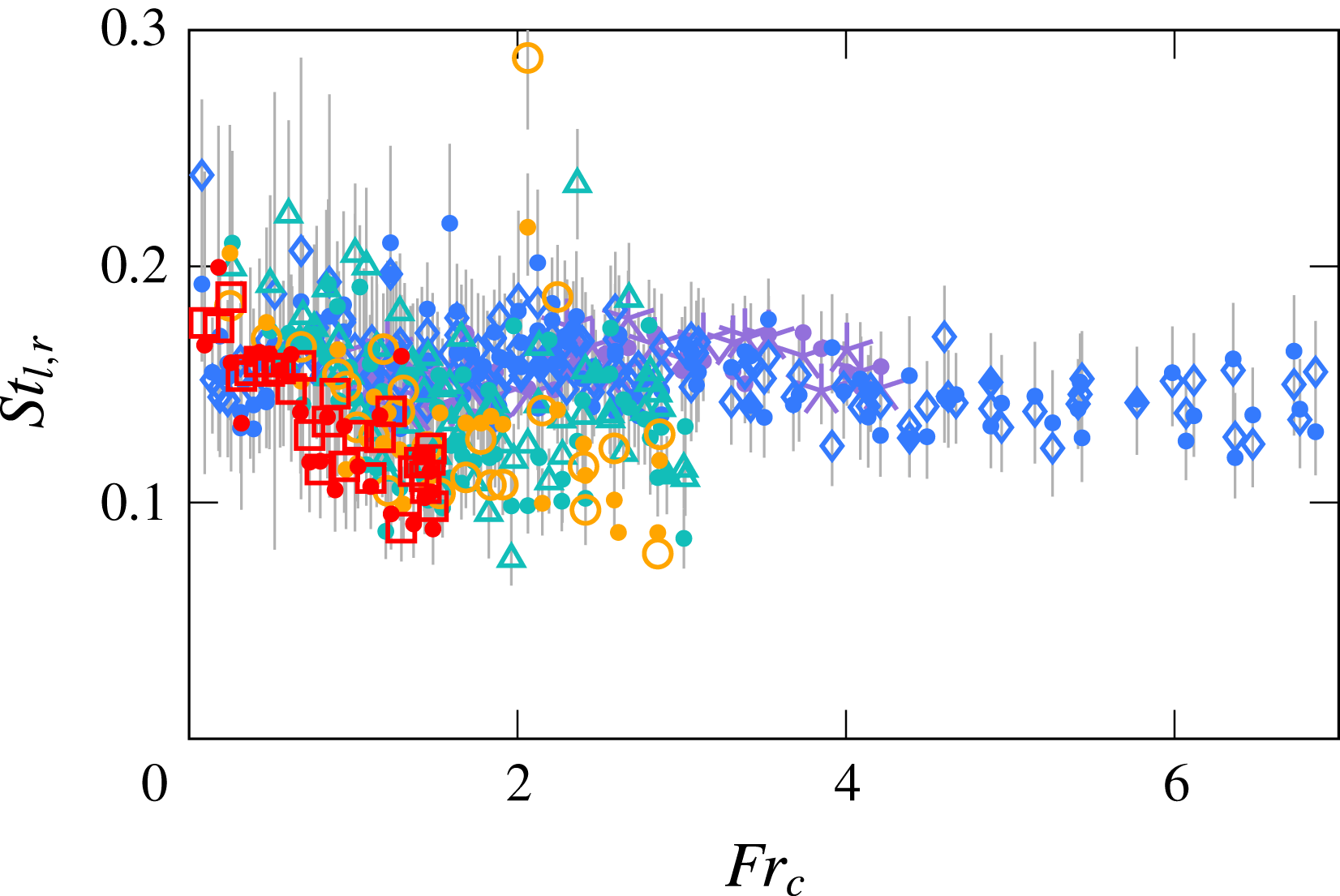
Left and right Strouhal numbers
 $St_{l,r}$
(4.5) are plotted against
 $Fr_{c}$
in figure 14. Note that we evaluated (4.5) based on the values of
 $f_{l,r}$
,
 $\hat{u} _{l,r}$
and
 $\overline{\unicode[STIX]{x1D706}}_{l,r}$
for each experiment, i.e. we did not use fitted power laws. Despite some scatter, the Strouhal numbers for our experiments convincingly fall within the band prescribed by Landel et al. (Reference Landel, Caulfield and Woods2012a
) and, to some extent, Rocco & Woods (Reference Rocco and Woods2015). For sets A and B (


 $St_{l,r}$
reach
 $0.12{-}0.16$
in the meandering regime. However, it is difficult to ascertain that all sets fall onto one line. Some level of discrepancy may point towards the relative inappropriateness of (4.5), in which we rely on experiment-averaged quantities to uncover the dynamics of temporally and spatially evolving structures. Notwithstanding, the range of our values for
 $St_{l,r}$
is consistent with previous studies on confined flows, with a level of scatter not unusual for this type of measurement.
As an aside, time series such as shown in figure 12(b,c) can be used to develop rigorous methods for separating the asymmetric–stable, transitional and meandering regimes. The streaks in figure 12(b) and (c), for instance, stagger, which is indicative of flapping, and hence of the meandering regime. In the asymmetric regime, where large-scale eddies form primarily on one side, one time series showcases many streaks, whereas the other showcases barely any. The transitional regime features a mixture of both behaviours. Thus, diagnostics can be built by subtracting one time series from the other and inspecting the distribution of peaks in the resulting matrix. Yet another method consists in tracking the centre of gravity
 $\{z_{g}(t),x_{g}(t)\}$
from ‘fluctuating’ snapshots such as figure 12(a) and inferring the regime from its trajectory. As stated in § 3 however, in the vast majority of cases, visual inspection suffices to distinguish regimes.
5 Conclusions
We have analysed, qualitatively and quantitatively, the behaviour of confined fountains for a wide range of governing parameters
 $Fr_{0}$
and
 $W/r_{0}$
. We have shown that confined fountains can be classified into four regimes, each characterised by slightly different interactions between the typical large-scale structures and the core of the fountain. The thresholds for these regimes can be delimited approximately by bands of a ‘confined’ Froude number
 $Fr_{c}\equiv Fr_{0}\,(W/r_{0})^{-5/4}$
as (see table 2):
(i) weakly confined regime:
$Fr_{c}\lesssim 1.1$
;(ii) asymmetric–stable regime:
$1.1\lesssim Fr_{c}\lesssim 1.8$
;(iii) transitional regime:
$1.8\lesssim Fr_{c}\lesssim 2.6$
;(iv) meandering (quasi-two-dimensional) regime:
$Fr_{c}\gtrsim 2.6$
.


The confined Froude number
 $Fr_{c}$
can be interpreted as a ratio between the height of the fountain, determined by
 $Fr_{0}$
, and its spanwise extent, restricted by
 $W$
; thus,
 $Fr_{c}$
expresses the level of confinement experienced by the fountain. Moreover, most quantities of interest, including the time-averaged rise height
 $\overline{z}_{f}$
(figure 8) and the average large-scale eddy size
 $\overline{\unicode[STIX]{x1D706}}_{l,r}$
(figure 11), scale on
 $WFr_{c}$
. Notably, the formation frequencies
 $f_{l,r}$
(figure 13) do not. Reasons for this are not fully understood and warrant further investigation.
The behaviour of confined fountains should be regarded as analogous to that of confined jets and plumes. As with other quasi-two-dimensional shear flows, large-scale eddies dominate and organise the flow. Their influence is somewhat more pronounced in fountains because of the finite vertical extent of the flow, which, furthermore, is comparable to the size of large-scale eddies.
Intriguingly, we did not observe any instance of more than two large-scale eddies being present simultaneously. When the eddies were distributed on both sides of the core, a serpentine S-shaped motion ensued in the core (e.g. figure 1). It would be interesting to see if, on increasing
 $Fr_{c}$
further, a greater number of eddies (and hence of winds in the core) could be achieved. The dimensions of our current set-up did not allow us to readily explore this possibility.
One outstanding open question regards the scaling of the rise height
 $\overline{z}_{f}$
. For the confinement ratios considered in this study, (4.2) represents an empirical fit which, accordingly, lies in excellent agreement with the data. The modest slope of
 $k_{s}$
at high values of
 $W/r_{0}$
suggests that (4.2) should remain valid at larger values of confinement ratio too. However, whilst it would be speculative to specify an upper bound for the validity of (4.2) in terms of
 $W/r_{0}$
(other than the conservative
 $W/r_{0}=24.2$
), it is clear that in the limit of no confinement,
 $W/r_{0}\rightarrow \infty$
, (4.2) does not apply. Ideally, a universal scaling law would be found that describes the transition from fully confined fountains to unconfined fountains. Such a law would be all but trivial: it would have to encompass regions of the
 $\{Fr_{0},W/r_{0}\}$
-space corresponding to fountains for which (i) the upflow has clung to the walls, (ii) only the counterflow has clung to the walls and (iii) only the induced flow is modified by confinement. The vast majority of our experiments fall within category (i), for which the scaling (4.2) seems appropriate in light of figures 8–11 and table 2.
Whilst we have mapped out the behaviour of confined fountains in terms of the principal governing parameters
 $\{Fr_{0},W/r_{0}\}$
, it would be informative to perform a study in which the source Reynolds number
 $Re_{0}$
was varied independently of
 $Fr_{0}$
. The vast majority of our experiments were conducted at moderate-to-high
 $Re_{0}$
, such that our results should be largely independent of
 $Re_{0}$
. Based on the work on unconfined round fountains by Burridge, Mistry & Hunt (Reference Burridge, Mistry and Hunt2015), one would indeed expect the influence of
 $Re_{0}$
to be secondary, provided
 $Re_{0}$
is reasonably high.
Finally, given the fountain’s intermittent nature, it is questionable whether a time-averaged theoretical modelling approach would lend much insight. It appears more promising instead to study the statistical distribution of the large-scale eddies (e.g. their trajectory, size and longevity) in order to better understand their role in organising the flow. This requires knowledge of velocity vectors. The next significant advance will therefore likely stem from more detailed measurements or from numerical simulations.
Acknowledgements
A.L.R.D. and G.R.H. would like to thank M. R. Slater and R. Leroy of the Fluid Dynamics Laboratory at the Cambridge University Engineering Department for their technical support in designing and manufacturing the experimental set-up. The authors would also like to thank the anonymous referees, whose comments helped shape the paper in its current form. In addition, funding from the UK Engineering and Physical Sciences Research Council under the grant number EP/L504920/1 and from the Qualcomm European Research Studentships in Technology is gratefully acknowledged.
Supplementary movies
Supplementary movies are available at https://doi.org/10.1017/jfm.2018.194.
Appendix A. Traces of volume flow rate
Given that many features of confined fountains display intermittency (most notably their large-scale eddies), it is essential to assure that this behaviour is not an artefact of fluctuations of the source flow rate
 $Q_{0}(t)$
. In this appendix, we demonstrate that fluctuations in
 $Q_{0}$
were small and, more importantly, that their dominant frequency does not correlate to the characteristic frequencies observed in the fountain.
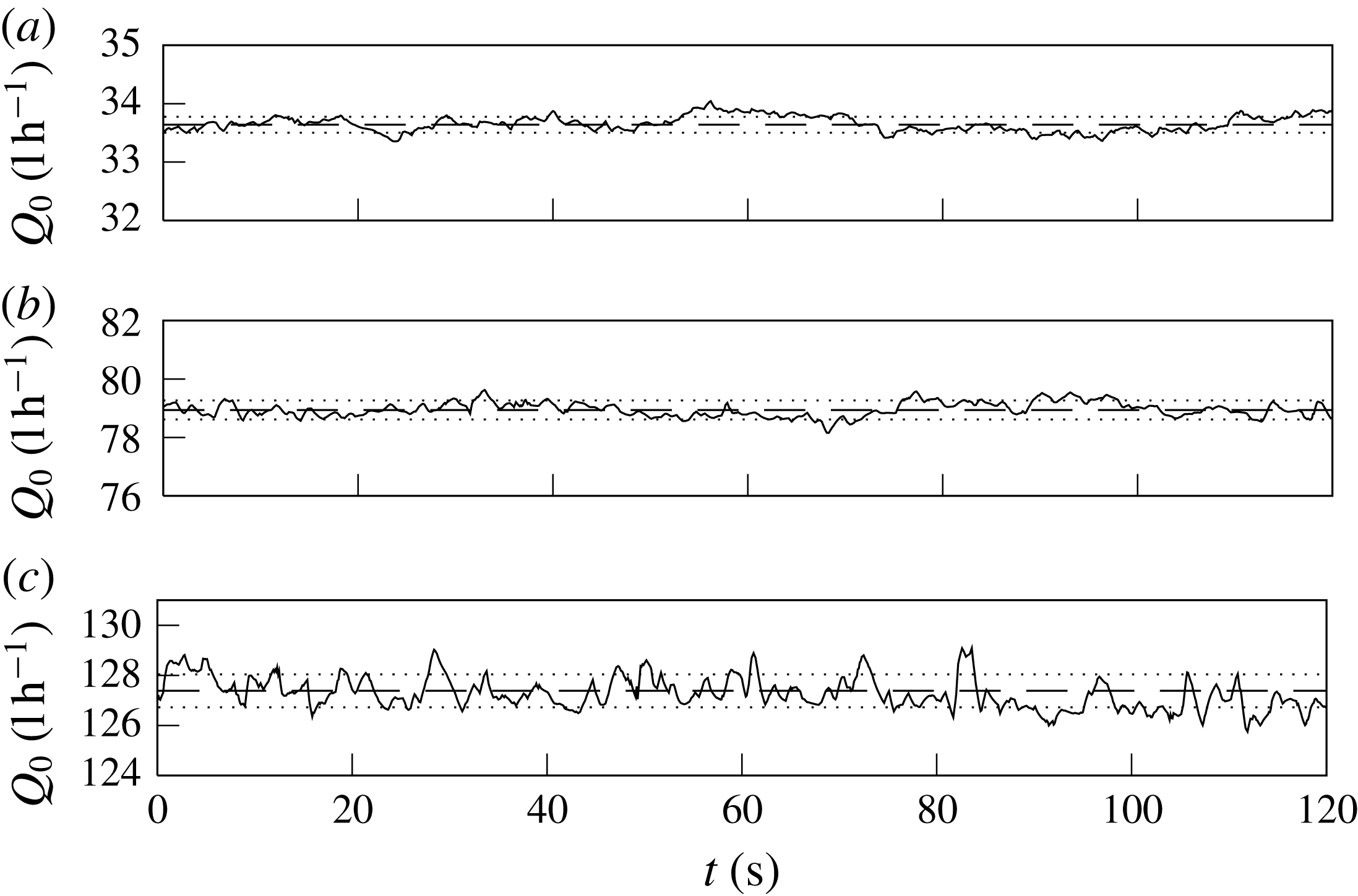
Typical traces of
 $Q_{0}(t)$
, here for (a)
 $\overline{Q}_{0}=33.6$
, (b)
 $78.9$
and (c)
 $127.4$
(
 $\text{l}~\text{h}^{-1}$
). Dashed lines represent experiment-averaged flow rates
 $\overline{Q}_{0}$
and dotted lines
 $\overline{Q}_{0}\pm \unicode[STIX]{x1D70E}(Q_{0})$
, where
 $\unicode[STIX]{x1D70E}$
denotes the standard deviation. For the three experiments shown,
 $\unicode[STIX]{x1D70E}(Q_{0})\leqslant 0.005\,\overline{Q}_{0}$
.

Three typical traces are plotted in figure 15 for small, moderate and high values of the time-averaged volume flow rate
 $\overline{Q}_{0}$
. These traces were recorded on an Altrato ‘Ultrasonic’ flow meter (accuracy
 $1.0\,\%$
) at a rate of
 $10~\text{Hz}$
. We provided back pressure to the flow circuit by inserting a ball valve downstream of the flow meter so as to minimise the formation of micro-bubbles, to which ultrasonic flow meters are susceptible. Whilst some erroneous readings (due to micro-bubbles) could not be prevented altogether, these readings were very short in duration (
 ${\sim}0.1~\text{s}$
) and did not affect the average.
From figure 15, it is evident that the source flow rate did not vary significantly over the course of a given experiment. Standard deviations across all recorded experiments rarely exceeded
 $1\,\%$
of the experiment-averaged flow rate
 $\overline{Q}_{0}$
. Moreover, the dominant frequencies associated with fluctuations such as seen in figure 15 lay around
 $0.03~\text{s}^{-1}$
, far from the frequencies that characterise the meandering motion in confined fountains (figure 13). (We extracted the dominant frequencies through fast Fourier transforms (FFT); see appendix D.) Less energetic peaks were also noted around
 $0.08{-}0.10~\text{s}^{-1}$
, closer to the formation frequencies of large-scale structures. However, it is unlikely that fluctuations at the source of magnitude
 ${<}0.01\,\overline{Q}_{0}$
should be responsible for the observed large-scale processes.
We conclude that the volume flow rate at the source was nominally constant and did not affect the observed flow features. Therefore, in the main text we drop the overbar notation and write
 $Q_{0}\equiv \overline{Q}_{0}$
.
Appendix B. Confined weak fountains
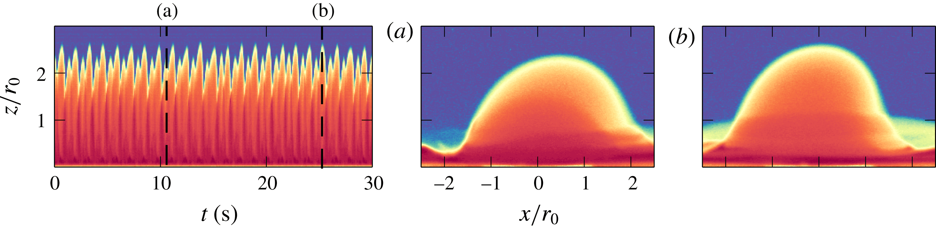
Confined weak fountains:
 $z_{f}(t)$
for
 $Fr_{0}=0.54$
(see supplementary movie 6). The fountain attaches to the front and back wall successively as it precesses around the source, resulting in a bimodal time series. Panels (a) and (b) depict a low peak and a high peak, respectively.

Weakly confined fountains (§ 3.1) are visually indistinguishable from their unconfined counterparts. From this resemblance, we concluded that the effects of confinement at
 $Fr_{0}\lesssim 8$
and
 $W/r_{0}=4.7$
were too weak to induce notable changes in dynamics. Whilst this observation remains true at moderate
 $Fr_{0}$
, in this appendix we report on weakly confined ‘weak’ fountains, for which
 $Fr_{0}$
is low (cf. the ‘weak’ unconfined fountains in the classification of Kaye & Hunt (Reference Kaye and Hunt2006)).
In the spirit of § 3, we use the unconfined Froude number
 $Fr_{0}$
instead of
 $Fr_{c}$
. Moreover, since weak fountains were (intentionally) only achieved at
 $W/r_{0}=4.7$
, we do not seek to generalise our results to
 $Fr_{c}$
.
For sufficiently weak releases (
 $Fr_{0}\lesssim 2$
at
 $W/r_{0}=4.7$
), where the gap width is larger than but comparable to the lateral extent of the fountain, the dynamics of weakly confined ‘weak’ fountains is distinct from their unconfined counterparts as a consequence of confinement. Unconfined fountains with these source conditions are known to circle and bob around the source (Williamson et al.
Reference Williamson, Srinarayana, Armfield, McBain and Lin2008). Here, this form of motion is impeded by the walls, thus to complete its ‘circles’ the fountain must periodically rise against the front and the back walls. This is illustrated by the time series for
 $\{Fr_{0}=0.54,\,Re_{0}=104\}$
(see supplementary movie 6) shown in figure 16. The response is regular and bimodal, each peak corresponding to the attachment of the fountain to the front and back wall.
As is common in the fountain literature, it appears that a finer subdivision of regimes might be appropriate for weak releases. This subdivision, however, is brought on by changes in
 $Fr_{0}$
, rather than by varying effects of confinement. Moreover, the fountain in figure 16 being clearly laminar, we expect that its dynamics will depend on the Reynolds number
 $Re_{0}$
(Williamson et al.
Reference Williamson, Srinarayana, Armfield, McBain and Lin2008). At low
 $Fr_{0}$
and low
 $Re_{0}$
, it therefore appears that weak fountains are more susceptible to
 $Fr_{0}$
and
 $Re_{0}$
than to
 $W/r_{0}$
. For this reason, we do not count ‘weak’ confined fountains as a separate regime in § 3 and opt to not further investigate them herein.
Appendix C. Gradients
$k_{s}$

It is well known that (unconfined) fountains scale on local flow variables: the subsequent rise height beyond some arbitrary height above the source
 $z^{\ast }$
, for instance, can be predicted based on the local Froude number
 $Fr(z^{\ast })$
(e.g. Hunt & Debugne 2016). In our experiments, the fountain evolves from being round at the source to being confined from a height
 $z=z_{a}$
onwards, where the flow attaches to the walls (the subscript ‘
 $a$
’ reading ‘attachment’). For
 $z>z_{a}$
, the fountain develops as a confined flow. Whilst the transition from the round source to the attachment height is determined by the source geometry and by entrainment, the subsequent rise of the confined fountain should scale on local variables which take into account confinement, i.e. on the local flow conditions at
 $z=z_{a}$
. Herein, we estimate these local flow conditions at attachment height based on the spreading rate and the dilution of a forced, round and, crucially, unconfined fountain. The ensuing scaling (C 4) is at odds with measurements, which highlights the necessity to perform more detailed measurements before a theoretical account of confined fountains (leading to (4.2)) can be derived.
We did not measure the attachment height
 $z_{a}$
or the internal variables at height
 $z_{a}$
in our experiments. However, as stated above, we may estimate
 $z_{a}$
and the internal variables on assuming that, prior to attachment, the flow behaves like a forced, unconfined and round fountain. (The assumption of a forced fountain is justified by our focus on high-
 $Fr_{0}$
fountains; see appendix B.) Then, for a round fountain whose radius
 $b$
spreads at a rate
 $b=2\unicode[STIX]{x1D6FC}z$
close to the source (Hunt & Debugne Reference Hunt and Debugne2016),
 $$\begin{eqnarray}\displaystyle b(z=z_{a})\approx \frac{W}{2}\quad \Rightarrow \quad z_{a}\approx \frac{W}{4\unicode[STIX]{x1D6FC}}. & & \displaystyle\end{eqnarray}$$
Based on our observations, all the fountains attached to the walls a short distance
 $O(W)$
above the source. Hence, it is advisable to treat
 $\unicode[STIX]{x1D6FC}$
in (C 1) as a problem-specific spreading coefficient which includes, e.g., the tendency of flows to cling to surfaces, rather than as a classic entrainment coefficient (Morton, Taylor & Turner Reference Morton, Taylor and Turner1956).
Following the same rationale as in (C 1), we assume a jet-like scaling near the source to infer the velocity at height
 $z_{a}$
as
 $$\begin{eqnarray}\displaystyle w_{a}\approx 2\,w_{0}\left(\frac{W}{r_{0}}\right)^{-1} & & \displaystyle\end{eqnarray}$$
and the reduced gravity at height
 $z_{a}$
from conservation of buoyancy (i.e. allowing the flow to dilute),
 $(r_{0}^{2}w_{0})g_{0}^{\prime }=[(W/2)^{2}w_{a}]g_{a}^{\prime }$
, as
 $$\begin{eqnarray}\displaystyle g_{a}^{\prime }\approx 2\,g_{0}^{\prime }\left(\frac{W}{r_{0}}\right)^{-1}. & & \displaystyle\end{eqnarray}$$
Finally, we combine the confined variables
 $b_{a}\equiv W/2$
,
 $w_{a}$
(C 2) and
 $g_{a}^{\prime }$
(C 3) into an ‘attachment’ Froude number
 $Fr_{a}$
, which describes the local flow conditions at
 $z=z_{a}$
, as
 $$\begin{eqnarray}\displaystyle Fr_{a}=\frac{w_{a}}{\sqrt{b_{a}\,g_{a}^{\prime }}}\approx 4\,Fr_{0}\left(\frac{W}{r_{0}}\right)^{-1}. & & \displaystyle\end{eqnarray}$$
Thus, based on the assumption that the flow prior to attachment behaves like a round fountain, (C 4) predicts that the rise heights of confined fountains should scale on
 $\overline{z}_{f}/W\propto Fr_{0}\,(W/r_{0})^{-1}$
. This implies that the gradients
 $k_{s}$
should follow
 $k_{s}\propto (W/r_{0})^{-1}$
.
To test the soundness of (C 4), we attempt to fit a curve of the type
 $k_{s}\propto (W/r_{0})^{-1}$
to the gradients in figure 8(a) (grey lines). While the general trend is well captured by the
 $-1$
power law, the gradients unmistakably fall onto two distinct curves: an upper curve for
 $W/r_{0}\leqslant 4.7$
(


 $k_{s}=2.50\,(W/r_{0})^{-1}$
, and a lower curve for
 $W/r_{0}\geqslant 11.8$
(▵, ◯, ▫), given by
 $k_{s}=1.61\,(W/r_{0})^{-1}$
. This corresponds to a relative difference in pre-factor of
 $44\%$
(taking the mean as a reference). This significant discrepancy implies that (C 4) and arguments leading up to (C 4) (i.e., that the flow may be treated as unconfined prior to attachment) oversimplify the actual dynamics of confined fountains. Notably, (C 4) neglects the effects of confinement altogether. A more sophisticated account, such as would emerge from measuring the inner variables at attachment height
 $w_{a}$
and
 $g_{a}^{\prime }$
, is probably required to retrieve the scaling (4.1). In the absence of such measurements, in the main text we proceed by adopting the empirical fit to our data (4.1).
Appendix D. Fourier transforms
In § 4.3, we presented an ‘eddy counting’ approach to identifying the formation frequencies of large-scale eddies. Encouragingly, the resulting frequencies agree well with these the naked eye discerns in experiments. In this appendix, we provide further confirmation of our approach by comparing its results to those obtained from Fourier transforms.
The signals
 $x_{l,r}(t)$
measure the lateral excursion of the fountain; in other words,
 $x_{l,r}(t)$
track the outer edge of large eddies when large eddies are present (figure 1). Thus, if these eddies form at a particular frequency, then this frequency should emerge from
 $x_{l,r}(t)$
as a dominant frequency, say
 $f_{{\mathcal{F}}(l,r)}$
.
We adopted the following procedure to reliably determine
 $f_{{\mathcal{F}}(l,r)}$
. First, we performed a Fourier transform using Matlab’s (R2015b) inbuilt FFT algorithm. The resulting signal (in the frequency domain) was then smoothed by applying a Savitzky–Golay filter of third order over a window of
 $\unicode[STIX]{x0394}f=\min [0.10,1.0/Fr_{0}]~\text{s}^{-1}$
(cf. Burridge & Hunt Reference Burridge and Hunt2013), which provided sufficient smoothing whilst retaining distinct peaks. For each experiment, the two frequencies associated with the largest amplitudes were sampled, and the highest of the two was denoted the ‘dominant frequency’,
 $f_{{\mathcal{F}}(l)}$
or
 $f_{{\mathcal{F}}(r)}$
, accordingly. To ensure that this dominant frequency had captured the trends underlying
 $x_{l,r}(t)$
, we then reconstructed the lateral motion by excluding any frequencies greater than
 $f_{{\mathcal{F}}(l,r)}$
and superimposed the reconstructed signal onto the original signal. This lent confidence that
 $f_{{\mathcal{F}}(l,r)}$
was indeed representative of the lateral motion.
Comparison between two methods for finding dominant frequencies in confined fountains: dominant frequencies
 $f_{{\mathcal{F}}(l,r)}$
, extracted from Fourier transforms of the signals
 $x_{l,r}(t)$
, superimposed on the formation frequencies
 $f_{l,r}$
identified by the ‘eddy counting’ approach (§ 4.3) in grey. Symbols as in figure 13.

Normalised characteristic (lateral) velocities for large-scale eddies
 $\hat{u} _{l,r}$
, obtained as the r.m.s. of the time derivative of
 $x_{l,r}(t)$
, the position of the outer edge of the eddy. Symbols as in figure 10.

The dominant frequencies thus extracted from the FFT are plotted separately in figure 17(a), and together with the frequencies obtained from the ‘eddy counting’ approach (faded) in figure 17(b). It is evident that both methods agree in trend as in magnitude. Although the FFT produces fewer outliers in set E, it also has greater scatter across all sets. Moreover, the interpretation of counting eddies is straightforward. Therefore, in the main text, we proceed to analyse the formation frequencies
 $f_{l,r}$
identified by counting eddies.
Appendix E. Characteristic velocities for large-scale eddies
Our aim in this appendix is to provide an estimate for the characteristic velocities of large-scale eddies. As alluded to in § 4.3, we calculate the characteristic velocities
 $\hat{u} _{l,r}$
by taking the r.m.s. of the derivative
 $\text{d}x_{l,r}/\text{d}t$
. Thus, we assume that the translational velocities at the edge of an eddy are representative of its overall velocity.
Care needs to be taken in applying the r.m.s. because
 $x_{l,r}(t)$
is not continuous everywhere. The signal
 $x_{l,r}(t)$
follows the farthermost edge of an eddy so long as that edge lies above
 $\overline{z}_{f}/2$
(§ 4.1) and, more generally, is within our field of vision. When the eddy leaves the field of vision, either sideways or downward,
 $x_{l,r}(t)$
appears to ‘jump’ abruptly as it rejoins the next candidate eddy. The eddy’s exit from the field of vision therefore causes discontinuities which will be interpreted as large and sudden variations in
 $x_{l,r}(t)$
. Whilst these discontinuities affect neither average excursions
 $\overline{x}_{l,r}$
nor frequencies
 $f_{{\mathcal{F}}(l,r)}$
, they introduce large artificial gradients which would be exacerbated by taking the r.m.s.
In order to avoid unphysical values of
 $\text{d}x_{l,r}/\text{d}t$
, we mark the time instants during which
 $x_{l,r}(t)$
is within three pixels of the boundaries of the field of vision left, right and downward. Subsequently, these time instants are excluded when calculating
 $\hat{u} _{l,r}=(\text{d}x_{l,r}/\text{d}t)_{rms}$
. A few outliers remain, which are screened out by excluding any gradient lying above or below three standard deviations.
The resulting characteristic velocities
 $\hat{u} _{l,r}$
, normalised by the buoyancy-induced velocity
 $\sqrt{g_{0}^{\prime }W}$
, are plotted against
 $Fr_{0}$
in figure 18. The scaling
 $\sqrt{g_{0}^{\prime }W}$
is inherited from unconfined fountains, where velocities scale as
 $\sqrt{g_{0}^{\prime }r_{0}}$
(e.g. Hunt & Debugne 2016). Characteristic velocities mirror the classification into regimes (§ 3), again splaying in the asymmetric and transitional regimes before merging in the meandering regime. However, no clear power law emerged from
 $\hat{u} _{l,r}$
, hence we did not explore the scaling further.