2 Overview of periodic (WEC) systems

We consider systems where a sub-array ${\mathcal{A}}$ of $N$ three-dimensional oscillating, energy-extracting bodies is periodically repeated along one dimension, say in the $y$ -direction, figure 1(a). The spacing between the repeated sub-arrays or, equivalently, the width of a basic cell containing the sub-array, is defined as periodicity  $d$ . The spatial configuration ${\mathcal{C}}$ of a periodic array specifies the positions of the bodies in ${\mathcal{A}}$ and periodicity  $d$ . We use the term ‘row’ to refer to a subset of the entire array, which consists of only one body from ${\mathcal{A}}$ periodically repeated. The water depth $h$ is assumed constant. The array interacts with an inviscid, monochromatic plane wave (angular frequency  $\unicode[STIX]{x1D714}$ , wavenumber  $k$ , amplitude  $A$ ) that propagates at an incident angle $\unicode[STIX]{x1D703}_{I}$ relative to the array normal ( $x$ -axis). We consider here the case of small wave steepness ( $kA\ll 1$ ) and small body motion, so the system can be studied in the context of linear potential flow.

Figure 1.

(a) Top view of the spatial configuration of a periodic array of sub-arrays ${\mathcal{A}}$ with $N=3$ bodies; periodicity is denoted by  $d$ . (b) Side view of the problem. (c) Scattering mode directions $\unicode[STIX]{x1D703}_{m}$ in the far field. The array is represented by the grey strip.

The problem is governed by the three-dimensional Laplace equation $\unicode[STIX]{x1D6FB}^{2}\unicode[STIX]{x1D6F7}=0$ , where $\unicode[STIX]{x1D6F7}(x,y,z)$ is the complex velocity potential (the real-valued velocity potential is  $\hat{\unicode[STIX]{x1D6F7}}(x,y,z,t)=\text{Re}(\unicode[STIX]{x1D6F7}\text{e}^{-\text{i}\unicode[STIX]{x1D714}t})$ ). The linear dynamic–kinematic boundary on the free surface leads to the dispersion relation $\unicode[STIX]{x1D714}^{2}=gk\tanh kh$ ( $g$ is the acceleration of gravity). In the open domain, i.e. away from the virtual vertical cylinders containing each body, the depth dependence can be factored out; consequently, the three-dimensional Laplace equation reduces to the two-dimensional Helmholtz equation $\unicode[STIX]{x1D6FB}_{H}^{2}\unicode[STIX]{x1D6F7}+k^{2}\unicode[STIX]{x1D6F7}=0$ , where $\unicode[STIX]{x1D735}_{H}=(\unicode[STIX]{x2202}_{x},\unicode[STIX]{x2202}_{y})$ is the gradient operator in the horizontal plane.

In addition to the standard boundary conditions on the body surfaces and the bottom ( $z=-h$ ) (Mei, Stiassnie & Yue Reference Mei, Stiassnie and Yue2005), the potential $\unicode[STIX]{x1D6F7}$ satisfies the periodicity condition imposed by the periodicity of the underlying array. This condition is called Bloch theorem (Ashcroft & Mermin Reference Ashcroft and Mermin1976), and it states that in a periodic system the values of a field at equivalent locations in two different cells differ only in the phase caused by the incident wave at those locations. For periodic arrays considered here, the Bloch theorem reads

(2.1) $$\begin{eqnarray}\unicode[STIX]{x1D6F7}(x,y+d,z)=\text{e}^{\text{i}\unicode[STIX]{x1D6FD}d}\unicode[STIX]{x1D6F7}(x,y,z),\end{eqnarray}$$

where $\unicode[STIX]{x1D6FD}\equiv k\sin \unicode[STIX]{x1D703}_{I}$ . $\unicode[STIX]{x1D6FD}$ is the component of the wavevector along the array (also known as the Bloch wavenumber or as the crystal wavevector in solid-state physics).

The periodic nature of the problem requires that only plane waves are present in the far field, and are allowed to propagate in certain directions only. The propagation directions $\unicode[STIX]{x1D703}_{m}$ depend solely on the periodicity  $d$ , wavenumber $k$ and the incident angle $\unicode[STIX]{x1D703}_{I}$ and are governed by the grating equation (e.g. Twersky Reference Twersky1956; Falnes & Budal Reference Falnes and Budal1982; Maystre Reference Maystre, Enoch and Bonod2012)

(2.2) $$\begin{eqnarray}\sin \unicode[STIX]{x1D703}_{m}=\sin \unicode[STIX]{x1D703}_{I}+\frac{2\unicode[STIX]{x03C0}}{kd}m,\quad m=0,\pm 1,\pm 2,\ldots .\end{eqnarray}$$

Here, the index $m$ denotes the scattering mode, i.e. a planar wave propagating in direction $\unicode[STIX]{x1D703}_{m}$ with amplitude $A_{m}$ in the far field. We consider incident waves that are propagating from the left half-plane ( $-\unicode[STIX]{x03C0}/2<\unicode[STIX]{x1D703}_{I}<\unicode[STIX]{x03C0}/2$ ), so the transmitted waves are plane waves occupying the right half-plane, and the reflected waves the left one. We denote the transmitted wave properties as $\unicode[STIX]{x1D703}_{m}^{+}$ and  $A_{m}^{+}$ , and the reflected wave properties as $\unicode[STIX]{x1D703}_{m}^{-}$ and $A_{m}^{-}$ . Note that $\unicode[STIX]{x1D703}_{m}^{+}\equiv \unicode[STIX]{x1D703}_{m}$ and $\unicode[STIX]{x1D703}_{m}^{-}\equiv \unicode[STIX]{x03C0}-\unicode[STIX]{x1D703}_{m}$ ; in particular $\unicode[STIX]{x1D703}_{0}^{+}=\unicode[STIX]{x1D703}_{I}$ and $\unicode[STIX]{x1D703}_{0}^{-}=\unicode[STIX]{x03C0}-\unicode[STIX]{x1D703}_{I}$ (mirror reflection).

As evident from (2.2), when the value of $kd$ increases past a certain critical value, a new scattering mode appears in the far field. The emergence of, say, the $m$ th mode occurs when $|\text{sin}\,\unicode[STIX]{x1D703}_{m}|=1$ , resulting in the critical wavenumber $(kd)_{m}^{cr}$

(2.3) $$\begin{eqnarray}(kd)_{m}^{cr}=m\frac{2\unicode[STIX]{x03C0}}{\pm 1-\sin \unicode[STIX]{x1D703}_{I}}.\end{eqnarray}$$

The new mode emerges at the so-called grazing angle $|\unicode[STIX]{x1D703}_{m}|=\unicode[STIX]{x03C0}/2$ , i.e. it propagates along the grating. A further increase in $kd$ past $(kd)_{m}^{cr}$ results in aligning $\unicode[STIX]{x1D703}_{m}^{+}$ closer to $\unicode[STIX]{x1D703}_{I}$ (or for reflected waves $\unicode[STIX]{x1D703}_{m}^{-}$ closer to $\unicode[STIX]{x03C0}-\unicode[STIX]{x1D703}_{I}$ ). For $\unicode[STIX]{x1D703}_{I}>0$ , the lowest critical wavenumber occurs for $m=-1$ . We denote by ${\mathcal{M}}$ the set of all indices of the propagating modes in the far field

(2.4) $$\begin{eqnarray}{\mathcal{M}}(\unicode[STIX]{x1D703}_{I},kd)=\left\{m:\left|\text{sin}\,\unicode[STIX]{x1D703}_{I}+\frac{2\unicode[STIX]{x03C0}m}{kd}\right|<1,m\in \mathbb{Z}\right\}.\end{eqnarray}$$

The scattered free surface $\unicode[STIX]{x1D702}_{S}$ in the far field can then be written as a superposition of planar waves propagating in directions  $\unicode[STIX]{x1D703}_{m}$ :

(2.5) $$\begin{eqnarray}\unicode[STIX]{x1D702}_{S}^{\pm }=\mathop{\sum }_{m\in {\mathcal{M}}}A_{m}^{\pm }\text{e}^{\text{i}kr\cos (\unicode[STIX]{x1D717}-\unicode[STIX]{x1D703}_{m}^{\pm })},\quad r|\cos \unicode[STIX]{x1D717}|\rightarrow \infty ,\end{eqnarray}$$

where $(r,\unicode[STIX]{x1D717},z)$ is a cylindrical coordinate system centred at the origin.

When a new scattering mode appears, there is a redistribution of energies (or, equivalently, of amplitudes $|A_{m}|$ ) among the existing scattering modes, generally resulting in abrupt changes in the performance. Rayleigh (1907) was the first to derive (2.3) as an attempt to describe the ‘anomalies’ in the optical diffraction spectrum of a metallic grating that were observed by Wood (Reference Wood1902). Although it was later shown that Rayleigh’s theory did not fully explain these Wood anomalies (Maystre Reference Maystre, Enoch and Bonod2012), the abrupt changes at $(kd)_{m}^{cr}$ in periodic systems are called Rayleigh anomalies (Hessel & Oliner Reference Hessel and Oliner1965). Although not strictly resonances, for terminological convenience, we hereafter refer to these anomalies as Rayleigh resonances, and we call $(kd)_{m}^{cr}$ (for a given  $d$ ) the ( $m$ th) Rayleigh wavenumber. In general, any $kd$ – $\unicode[STIX]{x1D703}_{I}$ combination for which a scattering mode of any order appears (i.e. for which the condition (2.3) holds) we call the ( $m$ th) Rayleigh critical condition. In fluid mechanics, Linton & Thompson (Reference Linton and Thompson2007) studied the resonant effects at the Rayleigh critical condition caused by an incident acoustic wave on a periodic array of cylinders.

In this study, we focus on the performance of lattice-like configurations of periodic arrays, rectangular-lattice arrays in particular. Here, lattice-like configurations refer to periodic arrays where the bodies are positioned according to the lattice vectors $\boldsymbol{a}_{\mathbf{1}}$ and $\boldsymbol{a}_{\mathbf{2}}=d\hat{\boldsymbol{e}}_{\boldsymbol{y}}$ , with only $N$ bodies in the $\boldsymbol{a}_{\mathbf{1}}$ direction (i.e. $N$ rows). For rectangular-lattice arrays (or rectangular arrays for brevity), $\boldsymbol{a}_{\mathbf{1}}=d_{x}\,\hat{\boldsymbol{e}}_{\boldsymbol{x}}$ , where $d_{x}$ is the row spacing. In addition, we consider arrays consisting of bodies of identical type only. We remark that the multiple-scattering framework presented in § 4 is valid for lattice and non-lattice periodic arrays alike, and possibly composed of different body types.

In terms of significant wave interaction effects, the prominent physical phenomena occurring in general lattice-like periodic arrays are Bragg and Laue scattering, which are well known in crystallography and solid-state physics (Ashcroft & Mermin Reference Ashcroft and Mermin1976). Bragg scattering is the occurrence of a strong reflection due to the constructive interference between the waves reflected from different rows in the lattice. It occurs when the condition (Bragg law)

(2.6) $$\begin{eqnarray}kd_{x}\cos \unicode[STIX]{x1D703}_{I}=n\unicode[STIX]{x03C0},\quad n=1,2,\ldots\end{eqnarray}$$

is satisfied. In the context of water waves, Bragg scattering effects have been studied for a wide range of problem domains, including periodic bottom ripples (Porter & Porter Reference Porter and Porter2003), periodic arrays of vertical cylinders (Li & Mei Reference Li and Mei2007a ) and periodic arrays of horizontal cylinders (Linton Reference Linton2011). Laue scattering, which is a generalization of Bragg scattering, is the condition when the incident wave and a scattered Rayleigh mode ( $m$ th one, say) are in such relationship that they are in phase at every lattice point (i.e. at every body). This condition is governed by the Laue equation

(2.7) $$\begin{eqnarray}(\boldsymbol{k}-\boldsymbol{k}_{m})\boldsymbol{\cdot }\boldsymbol{a}_{\mathbf{1}}=2\unicode[STIX]{x03C0}n,\quad n=1,2,\ldots ,\end{eqnarray}$$

where $\boldsymbol{k}$ is the wavevector of the incident wave, and $\boldsymbol{k}_{m}$ the wavevector of the $m$ th scattered mode.

A striking phenomenon that occurs at isolated wavenumbers in some periodic systems and that is also caused by wave interactions is the presence of embedded Rayleigh–Bloch waves. These waves are the solutions of the homogeneous boundary value problem that do not radiate to the far field, but stay ‘trapped’ around the array. Usually they are found as modes with frequency below the cutoff frequency for propagation in the far field and as such cannot couple with the incident wave field on a periodic system. (For finite arrays, these Rayleigh–Bloch modes can couple with the incident field, and are often called near-trapped waves as some of their energy ‘leaks’ away to the far field (e.g. Evans & Porter Reference Evans and Porter1997). This coupling has recently been applied to arrays with slowly varying properties (so-called ‘chirped’ or ‘graded’ arrays) to achieve large amplifications of the wave field inside the array for a wide spectrum of incident frequencies (Cebrecos et al. Reference Cebrecos, Picó, Sánchez-Morcillo, Staliunas, Romero-García and Garcia-Raffi2014; Bennetts, Peter & Craster Reference Bennetts, Peter and Craster2018).) In some rare cases, however, the Rayleigh–Bloch waves for periodic systems are found embedded in the continuous spectrum (Evans & Porter Reference Evans and Porter1998; McIver, Linton & McIver Reference McIver, Linton and McIver1998; Linton & McIver Reference Linton and McIver2007) so they can be excited by an incident wave, causing sharp changes in the array response. At the wavenumber $kd^{RB}$ at which an embedded Rayleigh–Bloch wave occurs, the response exhibits a sharp, narrow-banded jump; for wavenumbers away from the jump, the response is unaffected by its presence. The response values are significantly different for wavenumbers just below and above the jump wavenumber. When the response is plotted as a function of wavenumber, this results in an asymmetric response line shape relative to $kd^{RB}$ . These narrow-banded line shapes in the response are also called Fano features or resonances, after Fano (Reference Fano1941) who first discussed them as the (correct) explanation of Wood anomalies (Hessel & Oliner Reference Hessel and Oliner1965; Maystre Reference Maystre, Enoch and Bonod2012).

In WEC arrays, each body is connected to a power take-off (PTO) device, which converts the kinetic energy of the body motion into another, more useful, form. We consider here only linear PTO devices, i.e. those where the power take-off rate $b_{PTO}$ is the constant of proportionality between the device velocity and the force exerted by a PTO. For a body $j$ in a WEC array oscillating with a complex amplitude  $X_{j}$ , the mean extracted power $P_{j}$ (i.e. per one time period) is, thus

(2.8) $$\begin{eqnarray}P_{j}(\unicode[STIX]{x1D714})={\textstyle \frac{1}{2}}\unicode[STIX]{x1D714}^{2}b_{PTO}|X_{j}|^{2}.\end{eqnarray}$$

The mean extracted power of a periodic array $P_{a}=\sum _{j=1}^{N}P_{j}$ (per one cell) is the sum of the mean extracted powers by all the bodies in the sub-array  ${\mathcal{A}}$ . The most important quantity describing the performance of WEC arrays is the array gain  $q$ , which for a configuration ${\mathcal{C}}$ with $N$ identical WECs is defined as

(2.9) $$\begin{eqnarray}q(k,\unicode[STIX]{x1D703}_{I};{\mathcal{C}})=\frac{P_{a}(k,\unicode[STIX]{x1D703}_{I};{\mathcal{C}})}{NP_{\!iso}},\end{eqnarray}$$

where $P_{\!iso}$ is the power extracted by the same WECs operating in isolation. The capture width $W=P_{\!iso}/P_{w}$ of a body relates $P_{\!iso}$ with the power flux $P_{w}=(1/2)\unicode[STIX]{x1D70C}gA^{2}c_{g}$ of the incident wave. An optimal isolated WEC oscillating and extracting energy in heave achieves $kW=1$ (Evans Reference Evans1976; Mei et al. Reference Mei, Stiassnie and Yue2005). The capture width of an array $W_{a}=P_{a}/P_{w}$ is a measure of efficiency of available energy extraction, where $W_{a}=d\cos \unicode[STIX]{x1D703}_{I}$ indicates that all incident energy is extracted. In general, the array gain and the array capture width can be defined for arrays of heterogeneous WECs (both in terms of body geometry and extraction characteristics), as well as for directional irregular seas. For simplicity, we focus here only on the array gain for periodic arrays of identical WECs in monochromatic waves.

3 Performance of optimal rectangular-lattice point-absorber arrays

Before considering periodic arrays of general, finite-size WECs, we first consider rectangular periodic arrays with $N$ rows of point absorbers. Although the point-absorber approximation is strictly valid for small bodies ( $ka\ll 1$ ), this assumption simplifies the theoretical treatment and provides a useful foundation for studying periodic WEC arrays of bodies of general shape. The point-absorber theory for periodic arrays was developed by Srokosz (Reference Srokosz1980), Falnes & Budal (Reference Falnes and Budal1982) and Falnes (Reference Falnes1984). Here, we identify new underlying physical phenomena that were not recognized before, and discuss their effects. These phenomena serve as a basis for comparison with the performance of realistic periodic WEC arrays (in §§ 5 and 6).

For a rectangular periodic array of point absorbers where all the absorbers are heaving with the same amplitude, Falnes & Budal (Reference Falnes and Budal1982) derived an expression for the optimal gain  $\tilde{q}$

(3.1) $$\begin{eqnarray}\tilde{q}=Nkd\left[\mathop{\sum }_{m\in {\mathcal{M}}}\frac{S_{m,N}}{\cos \unicode[STIX]{x1D703}_{m}}\right]^{-1},\end{eqnarray}$$

where

(3.2) $$\begin{eqnarray}S_{m,N}=\frac{\sin ^{2}(Nkd_{x}(\cos \unicode[STIX]{x1D703}_{I}-\cos \unicode[STIX]{x1D703}_{m})/2)}{\sin ^{2}(kd_{x}(\cos \unicode[STIX]{x1D703}_{I}-\cos \unicode[STIX]{x1D703}_{m})/2)}+\frac{\sin ^{2}(Nkd_{x}(\cos \unicode[STIX]{x1D703}_{I}+\cos \unicode[STIX]{x1D703}_{m})/2)}{\sin ^{2}(kd_{x}(\cos \unicode[STIX]{x1D703}_{I}+\cos \unicode[STIX]{x1D703}_{m})/2)}.\end{eqnarray}$$

In order to achieve $\tilde{q}$ , the phases of motion amplitudes of individual point absorbers are determined from an optimality condition. Since the motion of the point absorbers is constrained to equal amplitudes, $\tilde{q}$ does not represent maximum achievable gain by a periodic array of point absorbers. Nevertheless, the existence of an explicit expression for $\tilde{q}$ provides a helpful insight into the phenomena that occur at certain wavenumbers – phenomena that exist in more general cases for which there is no such expression. For $N=1$ , however, the equal-amplitude constraint is no longer relevant, and (3.1) becomes the unconstrained optimal gain. The expression for $N=1$ was first derived by Srokosz (Reference Srokosz1980), for $\unicode[STIX]{x1D703}_{I}=0^{\circ }$ only.

We can obtain a general upper limit of gain, i.e. the maximum attainable array gain, by considering the incident energy flux on a general periodic WEC array. The maximum energy that any periodic WEC array can extract is limited by the normal component of the incident energy flux, resulting in the maximum array capture width $(W_{a})_{max}=d\cos \unicode[STIX]{x1D703}_{I}$ . Since the array gain can equivalently be expressed as $q=W_{a}/NW$ and the maximum capture width of a heaving isolated body is $(kW)_{max}=1$ , we obtain the maximum attainable gain $q_{max}$ for an array with $N$ rows

(3.3) $$\begin{eqnarray}q_{max}=\frac{kd}{N}\cos \unicode[STIX]{x1D703}_{I},\end{eqnarray}$$

relative to the optimal isolated absorbers. This expression is valid for general bodies and general heave amplitudes (if non-heave motion or additional degrees of freedom of motion are considered and $(kW)_{max}$ is increased (e.g. Evans Reference Evans1976), $q_{max}$ will be proportionally reduced). As such, (3.3) is also valid for the point-absorber arrays studied in this section, and $q_{max}$ can be recognized as the maximum achievable $\tilde{q}$ from (3.1). Since both $S_{m,N}$ and $\cos \unicode[STIX]{x1D703}_{m}$ are greater than or equal to zero, $\tilde{q}$ is maximum when the denominator is kept to a single ( $m=0$ ) term. For $m=0$ , (3.2) becomes

(3.4) $$\begin{eqnarray}S_{0,N}=N^{2}+\frac{\sin ^{2}(Nkd_{x}\cos \unicode[STIX]{x1D703}_{I})}{\sin ^{2}(kd_{x}\cos \unicode[STIX]{x1D703}_{I})},\end{eqnarray}$$

which results in $q_{max}=\tilde{q}$ for cases when the fraction in (3.4) is zero, i.e. when

(3.5) $$\begin{eqnarray}kd_{x}\cos \unicode[STIX]{x1D703}_{I}=\frac{n\unicode[STIX]{x03C0}}{N},\quad n=1,\ldots ,N-1.\end{eqnarray}$$

The expression (3.3) is intuitively understandable – increasing the number of rows $N$ decreases $q_{max}$ as back rows can extract relatively less energy when the front ones are extracting as much as possible. Non-normal incident angles also reduce $q_{max}$ , proportionally to the reduction in the energy flux across the array. An increase in  $kd$ , on the other hand, leads to an increase in $q_{max}$ as the performance of an isolated absorber can potentially be significantly improved through favourable wave interactions occurring in arrays. This potential, however, is difficult to attain for most (especially greater) $kd$ values.

Evaluating $\tilde{q}$ for a range of $kd$ values and for specific $d_{x}/d$ , $N$ and $\unicode[STIX]{x1D703}_{I}$ values reveals that $\tilde{q}$ undergoes significant oscillations, but also possesses some consistent features, figure 2. The complex oscillatory behaviour of $\tilde{q}$ as a function of wavenumber $kd$ increases with  $kd$ , $d_{x}/d$ , and  $N$ . At every Rayleigh wavenumber $(kd)_{m}^{cr}$ , $\tilde{q}$ drops abruptly to zero. Mathematically, this follows from the emergence of a new mode at $|\unicode[STIX]{x1D703}_{m}|=\unicode[STIX]{x03C0}/2$ , causing (one of the terms in the sum in) the denominator in (3.1) to become unbounded. For $N>1$ , $\tilde{q}=q_{max}$ for some wavenumbers, in which case all the incident energy is extracted ( $W_{a}=d$ ). This mostly occurs for wavenumbers below the first Rayleigh wavenumber $(kd)_{1}^{cr}$ (i.e. (3.5) holds). For larger $kd$ values, $\tilde{q}$ in general does not achieve $q_{max}$ , but the values of $\tilde{q}$ get larger as $q_{max}$ increases. Note that $\tilde{q}$ for single-row arrays never attains $q_{max}$ – it is at most $\tilde{q}=0.5\,q_{max}$ (for $kd$ below $(kd)_{1}^{cr}$ ), confirming that $(W_{a}/d)_{max}=0.5$ for a single-row array (Srokosz Reference Srokosz1980).

Figure 2.

Array gain $\tilde{q}$ as a function of $kd$ for $\unicode[STIX]{x1D703}_{I}=0^{\circ }$ for rectangular periodic point-absorber arrays of different aspect ratios $d_{x}/d$ . The vertical dashed lines at $kd=\text{const.}$ denote Rayleigh critical conditions. The sloped dashed coloured lines denote the maximum achievable gain $q_{max}$ . Note that $\tilde{q}$ for the single-row array ( $N=1$ ) is unaffected by $d_{x}/d$ and is shown as a reference in both plots.

We can gain an insight into the complex variation of $\tilde{q}$ with $kd$ by considering the underlying wave interaction mechanisms in periodic arrays. We argue here that there are three important phenomena that lead to a significant reduction in array gain – (i) the aforementioned Rayleigh resonances due to the emergence of new scattering modes; (ii) Bragg resonances occurring for lattice-like arrays of $N>1$ rows; and (iii) Laue resonances occurring in lattice-like arrays of $N>1$ rows when one or more scattering modes are present. The first two of these effects were already studied, with some limitations, in the literature, as discussed in § 1. The third phenomenon – Laue resonances – has not been previously discussed in the context of WEC arrays. (A different type of Laue scattering in the context of doubly periodic arrays of bottom-mounted cylinders was studied by Li & Mei Reference Li and Mei2007b .)

We argue that for WEC arrays, Laue interference results in a reduced surface elevation at the bodies, leading to a reduced array gain. The Laue equation (2.7) for rectangular periodic arrays with $\boldsymbol{a}_{\mathbf{1}}=d_{x}\,\hat{\boldsymbol{e}}_{\boldsymbol{x}}$ becomes

(3.6) $$\begin{eqnarray}kd_{x}(\cos \unicode[STIX]{x1D703}_{I}-\cos \unicode[STIX]{x1D703}_{m})=2\unicode[STIX]{x03C0}n,\quad n=1,2,\ldots .\end{eqnarray}$$

Mathematically, we recognize that (3.6), when approaching the limit, is the condition that would make the first fraction in (3.2) become $N^{2}$ , thus reducing $\tilde{q}$ . We refer to (3.6) (and to (2.7)) as Laue resonance conditions, and label these resonances according to indices $(m,n)$ . Note that this is purely an array-configuration-type resonance and is independent of body type and body resonances. The Bragg resonance condition (2.6) can be seen as a special case of Laue equation when $\unicode[STIX]{x1D703}_{m}=\unicode[STIX]{x1D703}_{0}^{-}=\unicode[STIX]{x03C0}-\unicode[STIX]{x1D703}_{I}$ , i.e. when there is strong reflection as a result of interference of the incident and the reflected wave.

To help elucidate the structure of optimal array gain, we plot the contours of $\tilde{q}$ in $kd_{x}$ – $kd$ space, figure 3. The domain is criss-crossed by well-defined lines along which $\tilde{q}$ is noticeably reduced – these lines represent Rayleigh, Bragg and Laue resonances. Rayleigh wavenumbers $(kd)_{m}^{cr}$ , calculated from (2.3), are the horizontal lines across which there is an abrupt change in $\tilde{q}$ – (cf. figure 2). Bragg resonances are the vertical, equispaced lines, calculated from (2.6), along which there is a reduction in  $\tilde{q}$ . Laue resonances are the family of curved lines, obtained from (3.6) for each Rayleigh–Bragg $(m,n)$ pair, along which $\tilde{q}$ is also reduced. For a particular $(m,n)$ -Laue-resonance curve, the line asymptotes to a vertical for small $kd_{x}$ . For $\unicode[STIX]{x1D703}_{I}=0$ , this vertical is the $n$ th Bragg line. For large $kd_{x}$ , the Laue resonance curve grows monotonically with $kd_{x}$ . At the intersection with the $2n$ th Bragg line, the $(m,n)$ Laue curve is tangent to the $m$ th Rayleigh critical condition line. Where several Laue resonances coincide, the decrease in $\tilde{q}$ is more pronounced – at the particular $kd$ – $kd_{x}$ value as well as for the values around it. As $kd$ and $kd_{x}$ are increased, Laue resonances become progressively denser, increasing the portion of the domain where $\tilde{q}$ is significantly reduced (relative to $q_{max}$ ). Increasing the number of bodies $N$ in the array decreases the overall $\tilde{q}$ , as expected from (3.3), and the troughs in $\tilde{q}$ caused by Bragg and Laue resonances become narrower. Increasing the incident angle $\unicode[STIX]{x1D703}_{I}$ reduces the overall $\tilde{q}$ (in accordance with (3.3)). Furthermore, the non-normal incident angle results in a larger number of distinctive Rayleigh modes, thus increasing the number (i.e. the density) of Laue resonances and, as a result, further reducing $\tilde{q}$ in an increased portion of the domain (relative to normal incidence).

Figure 3.

Contours of array gain $\tilde{q}$ for rectangular periodic point-absorber arrays of $N=3$ (a,b) and $N=5$ (c,d) rows; each column corresponds to one incident angle $\unicode[STIX]{x1D703}_{I}$ . Horizontal green lines represent Rayleigh critical conditions, vertical (grey) lines Bragg resonances and magenta lines Laue resonances. Note that some of the ‘high-frequency’ oscillations in $\tilde{q}$ (cf. figure 2) are smoothed when plotted as contours due to the limited image resolution.

The optimal gain $\tilde{q}$ as a function of $kd_{x}$ is shown is figure 4, for two incident angles ( $\unicode[STIX]{x1D703}_{I}=0^{\circ },15^{\circ }$ ) and two $kd$ values. Here, we recognize Bragg resonances as troughs in $\tilde{q}$ at $kd_{x}$ values given by (2.6). Unlike $\tilde{q}$ at the Rayleigh critical points, $\tilde{q}$ at Bragg resonances exhibits smooth behaviour. For $kd$ below the lowest Rayleigh wavenumber  $(kd)_{-1}^{cr}$ (figure 4 a,b), $\tilde{q}$ oscillates between a minimum value $\tilde{q}_{min}$ – which occurs at Bragg resonances (2.6) – and $q_{max}$ . In between Bragg resonances, $\tilde{q}$ achieves $N-1$ peaks, given by (3.5). We can calculate $\tilde{q}_{min}$ from $S_{0,N}$ by using the Bragg condition (2.6), giving

(3.7) $$\begin{eqnarray}\tilde{q}_{min}=\frac{kd}{2N}\cos \unicode[STIX]{x1D703}_{I}=\frac{q_{max}}{2}.\end{eqnarray}$$

If an additional scattering mode is present (i.e. $kd>(kd)_{-1}^{cr}$ ), the maximum values of $\tilde{q}$ reach $q_{max}$ only for large values of $kd_{x}$ (figure 4 c,d). In these cases, deep troughs away from Bragg resonances are the result of Laue resonances. A particularly prominent reduction in $\tilde{q}$ at $kd_{x}=5\unicode[STIX]{x03C0}$ in figure 4(c) is a result of combined Bragg, and $(1,1)$ - and $(1,4)$ -Laue resonances. Bragg resonances are also clearly visible in figure 2 for the $d_{x}/d=1.5$ , $N>1$ arrays as two prominent, smooth dips in $\tilde{q}$ for $kd<(kd)_{1}^{cr}$ .

Note that troughs at Bragg resonances are pronounced even for a two-row array ( $N=2$ ), indicating that strong reflection occurs at these conditions. This is different from the Bragg-resonance-related decrease in performance found by Garnaud & Mei (Reference Garnaud and Mei2010), where, because of the weak-absorber assumption, significant effects due to Bragg resonance accumulate only after a large number of rows.

Figure 4.

Array gain $\tilde{q}$ for rectangular periodic point-absorber arrays of $N$ rows as a function of $kd_{x}$ , for $kd=\unicode[STIX]{x03C0}$ (a,b) and $kd=2.5\unicode[STIX]{x03C0}$ (c,d) and $\unicode[STIX]{x1D703}_{I}=0^{\circ }$ (a,c) and $\unicode[STIX]{x1D703}_{I}=15^{\circ }$ (b,d). Bragg resonances are marked by dashed vertical lines. Thin horizontal lines in corresponding colour mark the maximum attainable gain $q_{max}$ for each $N$ (in (c) and (d) the $q_{max}$ line for $N=2$ is outside the presented range).

Figure 5.

Array gain $\tilde{q}$ in the presence of matched Rayleigh–Bragg resonances as a function of $kd$ for three different configurations of rectangular periodic point-absorber arrays with $N=3$ rows ( $\unicode[STIX]{x1D703}_{I}=0^{\circ }$ ). Rayleigh resonances in these cases always occur every $2\unicode[STIX]{x03C0}$ in this figure; matched Rayleigh–Bragg resonances are marked by red vertical lines; isolated Bragg resonances are marked by green vertical lines. Notice that the asymmetry in $\tilde{q}$ for wavenumbers $kd$ just above and below the matched resonances (red lines) is much smaller than that around the isolated Rayleigh resonances.

The sharp, abrupt changes in $\tilde{q}$ at Rayleigh wavenumbers are in contrast to the smooth, symmetric behaviour of $\tilde{q}$ around Bragg resonances. However, Rayleigh and Bragg resonances can occur together at the same wavenumber (figure 3), and it is of interest to study how $\tilde{q}$ is affected by these contrasting behaviour patterns. We call this condition matched Rayleigh–Bragg resonance, and its existence depends solely on the array configuration $d_{x}/d$ . For normal incidence, if $d_{x}/d$ is a rational number, there exist wavenumbers for which the matched Rayleigh–Bragg resonance occurs. Among the set of rational numbers, the arrays with $d_{x}/d=1/2$ are special in that Rayleigh and Bragg resonances always occur together, i.e. every occurrence of a Rayleigh resonance is accompanied by a Bragg resonance and vice versa. For $d_{x}/d<1/2$ , there are isolated Rayleigh resonances, and for $d_{x}/d>1/2$ there are isolated Bragg resonances. In figure 5, we show $\tilde{q}$ for three-row periodic point-absorber arrays of different configurations $d_{x}/d$ at normal incidence. We contrast the response at matched Rayleigh–Bragg resonances with that at isolated Rayleigh and Bragg resonances. When a matched Rayleigh–Bragg resonance occurs, $\tilde{q}$ still exhibits a sharp, narrow-banded drop to zero as for an isolated Rayleigh resonance, but $\tilde{q}$ values for wavenumbers below and above the resonance are more similar. As a result, the behaviour of $\tilde{q}$ across the matched Rayleigh–Bragg is smoothed out.

Finally, we remark that the physics behind Laue resonances relies on the lattice-like arrangement of the scatterers in a periodic array, so these resonances should exist in other lattice-like periodic WEC arrays, with similar effects. For example, for an oblique periodic array with the lattice vectors $\boldsymbol{a}_{\mathbf{1}}=(c\cos \unicode[STIX]{x1D6FE},c\sin \unicode[STIX]{x1D6FE})$ , the Laue-resonance condition (2.7) becomes

(3.8) $$\begin{eqnarray}kc(\cos (\unicode[STIX]{x1D703}_{I}-\unicode[STIX]{x1D6FE})-\cos (\unicode[STIX]{x1D703}_{m}-\unicode[STIX]{x1D6FE}))=2\unicode[STIX]{x03C0}n,\quad n=1,2,\ldots .\end{eqnarray}$$

The skewness of the array lattice in that case would affect the incidence angle at which Laue resonances are most prominent. Furthermore, the equal-amplitude constraint imposed on point-absorber arrays presented in this section is purely for mathematical convenience; we argue here and show in § 6 that the salient phenomena presented here also exist for lattice-like WEC arrays of finite-size bodies in unconstrained motion.

While the point-absorber theory provides a valuable insight into the absorption dynamics of periodic WEC arrays, it is an approximation that neglects several aspects (e.g. diffraction effects, evanescent waves) that are important for practical applications. We present a method that is capable of treating general, realistic WEC arrays next.

4 A direct algebraic method for general-shape multi-body periodic arrays

In this section, we present a new multiple-scattering method for periodic arrays consisting of sub-arrays of closely spaced bodies of arbitrary geometry. The approach is based on the Kagemoto & Yue (Reference Kagemoto and Yue1986) method for arrays with a finite number of bodies; it generalizes the formulation for a single-body periodic array (Peter et al. Reference Peter, Meylan and Linton2006) and that for periodic rows spaced far apart (Peter & Meylan Reference Peter and Meylan2009). It uses only the isolated body hydrodynamic coefficients, without the need for calculating those of the array itself. The method is applicable to fixed, freely oscillating or energy-extracting bodies in any number of degrees of freedom, or a combination thereof. The full formulation is somewhat involved with a number of important intermediate results, and the details are provided in appendix A. For clarity, we highlight below the key steps of the derivation and the main results.

Consider an infinite array formed by a periodically repeating sub-array ${\mathcal{A}}$ of $N$ bodies along the $y$ -axis with periodicity  $d$ , figure 6. The bodies ${\mathcal{B}}_{i}$ in the array are spaced far enough so that the virtual vertical cylinders that contain each body do not intersect (i.e. so that the potential outside the cylinders can be expressed in terms of cylindrical harmonics, see (A 4)); the spatial configuration of the sub-array ${\mathcal{A}}$ is otherwise without constraints. Each of the bodies ${\mathcal{B}}_{i}$ in ${\mathcal{A}}$ can be of an arbitrary shape. The position of body ${\mathcal{B}}_{j}$ is given by a vector $\boldsymbol{R}_{j}=(R_{j},\unicode[STIX]{x1D6FC}_{j})$ . A local cylindrical coordinate system $\boldsymbol{r}_{j}=(r_{j},\unicode[STIX]{x1D717}_{j},z)$ with the origin $O_{j}$ centred at the body ${\mathcal{B}}_{j}$ is defined for each body. The bodies can be fixed, or can be oscillating according to some known equation of motion.

Figure 6.

(a) Infinite array of periodically repeated sub-arrays of scatterers. The decomposition of the distance vector $\boldsymbol{R}_{\hat{\jmath }p}$ between the bodies ${\mathcal{B}}_{\hat{\jmath }}$ and ${\mathcal{B}}_{p}$ into $\boldsymbol{R}_{\hat{\jmath }j}$ and $\boldsymbol{R}_{jp}$ is shown. (b) Local coordinate systems of bodies ${\mathcal{B}}_{j}$ and ${\mathcal{B}}_{p}$ .

The standard approach in the multiple-scattering framework is to express the total potential as a sum of the incident wave potential and the unknown scattered wave potentials (and radiated wave potentials if the bodies are oscillating) for each of the bodies in the array. This can also be expressed relative to a particular body as the total incident potential for that body (consisting of the incident plane-wave potential and the scattered wave potentials of other bodies) and the scattered wave potential of that body alone. In order to determine the unknown potentials, we express the total incident and the scattered wave potential on a particular body in terms of partial waves (with propagating and evanescent radial components, and angular components), which are represented by a number of unknown coefficients that need to be determined. These coefficients can be represented by unknown vectors, say $\boldsymbol{c}^{p}$ and $\boldsymbol{d}^{p}$ for the scattered and the incoming wave potential on body  ${\mathcal{B}}_{p}$ , respectively. The goal is to express the incoming and scattered wave potentials on a body in terms of the same coordinate system so that the diffraction boundary condition imposed on that body can be used to determine the relationship between $\boldsymbol{c}^{p}$ and  $\boldsymbol{d}^{p}$ . Since the overall problem is linear, we can express that relationship in a matrix form as

(4.1) $$\begin{eqnarray}\boldsymbol{c}^{p}=\unicode[STIX]{x1D64F}^{p}\boldsymbol{\cdot }\boldsymbol{d}^{p},\end{eqnarray}$$

where $\unicode[STIX]{x1D64F}^{p}$ is the diffraction transfer matrix or $\unicode[STIX]{x1D64F}$ -matrix of body ${\mathcal{B}}_{p}$ (Kagemoto & Yue Reference Kagemoto and Yue1986; Martin Reference Martin2006). The $\unicode[STIX]{x1D64F}$ -matrix depends only on the body shape and is independent of the actual wave field around the body, so it can be pre-calculated (analytically or numerically) for a body in isolation. To solve the array problem, we express the unknown part of the incident potential on body ${\mathcal{B}}_{p}$ (i.e. the unknown part of $\boldsymbol{d}^{p}$ ) in terms of $\boldsymbol{c}^{p}$ and use (4.1) to close the system.

To express the potentials in terms of the same coordinate system, the standard approach is to use the Graf addition theorem for Bessel functions that result from partial wave decomposition of the potentials. The use of the addition theorem results in an expression that explicitly depends on distance vectors between the bodies; the distance vector $\boldsymbol{R}_{\hat{\jmath }p}$ between bodies ${\mathcal{B}}_{\hat{\jmath }}$ and ${\mathcal{B}}_{p}$ is shown in figure 6(a). However, unlike for the case of finite arrays, this approach applied to periodic arrays results in a summation over the infinite number of bodies across the cells. For single-row periodic arrays, Peter et al. (Reference Peter, Meylan and Linton2006) expressed the contributions from the infinite number of bodies in the form of rapidly converging lattice sum. For multiple, far-spaced rows, Peter & Meylan (Reference Peter and Meylan2009) used the far-field transmission and reflection matrices to account for the wave interactions between the rows.

In contrast to those efforts, we consider a general case where multiple rows can be closely spaced. To tackle the summation over the infinite number of bodies while accounting for the exact, near-field interaction between the bodies, we (i) use Bloch theorem (2.1) to transform the partial wave coefficients, (ii) decompose the distance vector $\boldsymbol{R}_{\hat{\jmath }p}$ as in figure 6(a) and (iii) use the Graf addition theorem again on the resulting vectors. This approach results in two separate summations. The first one accounts for the interactions among the bodies within a sub-array, and it depends only on the distance vectors $\boldsymbol{R}_{jp}$ between these bodies. The terms can be organized into a separation matrix $\unicode[STIX]{x1D64E}^{jp}$ (matrix elements given by (A 14)), which is identical to that for scattering by a finite, non-periodic array (Kagemoto & Yue Reference Kagemoto and Yue1986). The second summation accounts for the interactions among bodies across different cells, and is expressed in terms of a periodicity matrix $\unicode[STIX]{x1D64C}^{jp}$ (matrix elements given by (A 18) or (A 20)). The sum over the infinite number of cells in the periodicity matrix is expressed in a rapidly converging form (Linton Reference Linton1998).

As a result, all the potentials are expressed in the same coordinate system, and we use (4.1) to relate the scattered and incident wave coefficients. Thus, we obtain a linear system for the unknown coefficients of the scattered partial waves

(4.2) $$\begin{eqnarray}(\unicode[STIX]{x1D644}-\unicode[STIX]{x1D64F}(\unicode[STIX]{x1D64E}+\unicode[STIX]{x1D64C})^{\text{T}}\unicode[STIX]{x1D643})\boldsymbol{c}=\unicode[STIX]{x1D64F}\boldsymbol{d},\end{eqnarray}$$

where $\boldsymbol{c}$ , $\boldsymbol{d}$ , $\unicode[STIX]{x1D64F}$ , $\unicode[STIX]{x1D64E}$ , $\unicode[STIX]{x1D64C}$ , $\unicode[STIX]{x1D643}$ are the global block vectors and matrices representing scattered wave coefficients, incident planar wave coefficients, $\unicode[STIX]{x1D64F}$ -matrix, separation matrix, periodicity matrix and radiation transfer matrix, respectively; the superscript $(\cdot )^{\text{T}}$ denotes a matrix transpose. The expression (4.2) has several desirable properties. It is valid for bodies of general shape, not necessarily all equal. The bodies are allowed to be closely spaced, and the evanescent near field is fully taken into account. The bodies can be fixed or freely oscillating, and they can also extract energy.

The periodicity matrix $\unicode[STIX]{x1D64C}$ is a new addition to the original theory for non-periodic arrays. It depends on the periodicity $d$ of the array and the relative position of bodies in the sub-array ${\mathcal{A}}$ , but not on the properties or the motion of the bodies. For a periodic array with a single body ( $N=1$ ), $\unicode[STIX]{x1D64C}$ reduces to the well-known Schlömilch sum ((A 19); Linton Reference Linton1998; Peter et al. Reference Peter, Meylan and Linton2006). If we set $\unicode[STIX]{x1D64C}=\mathbf{0}$ , we recover the linear system for finite arrays (Kagemoto & Yue Reference Kagemoto and Yue1986).

The (global) radiation transfer matrix $\unicode[STIX]{x1D643}$ is another new component in our multiple-scattering formulation. It contains all the information about the dynamics and the radiation properties of the bodies. A body ${\mathcal{B}}_{p}$ is represented by an independent block  $\unicode[STIX]{x1D643}^{p}$

(4.3) $$\begin{eqnarray}\unicode[STIX]{x1D643}^{p}=\unicode[STIX]{x1D644}+{\unicode[STIX]{x1D658}^{\unicode[STIX]{x1D64D}}}^{p}\boldsymbol{\cdot }{\unicode[STIX]{x1D755}^{p}}^{\text{T}}\end{eqnarray}$$

in the global matrix $\unicode[STIX]{x1D643}$ , where ${\unicode[STIX]{x1D658}^{\unicode[STIX]{x1D64D}}}^{p}$ is a known matrix of coefficients of radiated waves for unit oscillation velocity of  ${\mathcal{B}}_{p}$ , and $\unicode[STIX]{x1D755}^{p}$ is the velocity transfer matrix. The velocity transfer matrix relates the complex oscillation velocity vector $\boldsymbol{V}_{}^{p}$ of the body ${\mathcal{B}}_{p}$ to the scattered wave coefficients through

(4.4) $$\begin{eqnarray}\boldsymbol{V}_{}^{p}={\unicode[STIX]{x1D755}_{}^{p}}^{\text{T}}\boldsymbol{\cdot }\boldsymbol{c}^{p}.\end{eqnarray}$$

This matrix is obtained from the equation of motion (A 27) for ${\mathcal{B}}_{p}$ , which, for multiple degrees-of-freedom motion, can be expressed as

(4.5) $$\begin{eqnarray}\unicode[STIX]{x1D63C}^{p}(\unicode[STIX]{x1D714})\boldsymbol{\cdot }\boldsymbol{X}^{p}=\boldsymbol{F}^{p}(\unicode[STIX]{x1D714},{\mathcal{C}}),\end{eqnarray}$$

where $\unicode[STIX]{x1D63C}^{p}$ is the body dynamics matrix (containing added mass and damping matrices for  ${\mathcal{B}}_{p}$ ), $\boldsymbol{X}^{p}$ the complex motion amplitude and $\boldsymbol{F}^{p}$ the total diffraction force on  ${\mathcal{B}}_{p}$ . Due to the linearity of wave–body interaction, the diffraction force on a body can be related to the coefficients $\boldsymbol{c}^{p}$ of the scattered partial waves by

(4.6) $$\begin{eqnarray}\boldsymbol{F}^{p}={\hat{\unicode[STIX]{x1D641}}^{p}\text{}}^{\text{T}}\boldsymbol{\cdot }\boldsymbol{c}^{p},\end{eqnarray}$$

where $\hat{\unicode[STIX]{x1D641}}^{p}$ is the diffraction force transfer matrix of body  $p$ , which can be calculated for a body in isolation. By relating the velocity to the motion amplitude $\boldsymbol{X}^{p}=\text{i}\boldsymbol{V}_{}^{p}/\unicode[STIX]{x1D714}$ and by using (4.4)–(4.6), we obtain the velocity transfer matrix as

(4.7) $$\begin{eqnarray}\unicode[STIX]{x1D755}_{}^{p}=-\text{i}\unicode[STIX]{x1D714}\hat{\unicode[STIX]{x1D641}}^{p}\boldsymbol{\cdot }(\unicode[STIX]{x1D63C}^{p})^{-1}.\end{eqnarray}$$

In this new formulation, only the isolated-body hydrodynamic coefficients (added mass, radiation damping) are required, while their array counterparts are never needed. The diffraction force on a body is dependent on the array configuration, but it is expressed through a configuration-independent transfer matrix $\hat{\unicode[STIX]{x1D641}}^{p}$ . The body dynamics is, thus, completely included and accounted for in the global system matrix (4.2), and both the hydrodynamics and the body dynamics are essentially solved simultaneously. Once the equation (4.2) is solved, the dynamics of any body can be trivially evaluated from (4.4).

For practical computations, we truncate the infinite system (4.2) to a sufficient number of evanescent and angular modes, denoted by $M$ and $N_{p}$ , respectively. With such truncation, $\boldsymbol{c}^{j}$ and $\boldsymbol{d}^{j}$ are of the size $M_{t}\times 1$ , where $M_{t}\equiv (2N_{p}+1)\times (M+1)$ , while $\unicode[STIX]{x1D64F}^{j}$ , $\unicode[STIX]{x1D64E}^{jp}$ , $\unicode[STIX]{x1D64C}^{jp}$ and $\unicode[STIX]{x1D643}^{j}$ are of the size $M_{t}\times M_{t}$ . The degree-of-freedom-dependent matrices $\hat{\unicode[STIX]{x1D641}}^{p}$ , ${\unicode[STIX]{x1D658}^{\unicode[STIX]{x1D64D}}}^{j}$ and $\unicode[STIX]{x1D755}_{}^{j}$ are of the size $M_{t}\times n_{DOF}$ , where $n_{DOF}$ is the number of degrees of freedom of the body. The total size of system matrices (i.e. $\unicode[STIX]{x1D64F},\unicode[STIX]{x1D64E},\unicode[STIX]{x1D64C},\unicode[STIX]{x1D643}$ ) is $NM_{t}\times NM_{t}$ , while the size of the scattered wave coefficient vector $\boldsymbol{c}$ for the entire system is $NM_{t}\times 1$ . The matrices $\unicode[STIX]{x1D64F}$ and $\unicode[STIX]{x1D643}$ depend only on the isolated-body properties, and can be pre-calculated. If the spatial configuration of the sub-array is changed, only the separation matrix $\unicode[STIX]{x1D64E}$ and the periodicity matrix $\unicode[STIX]{x1D64C}$ need to be re-evaluated, requiring $O(N^{2})$ effort. Since $N$ is usually very small ( $N\lesssim 10$ ), these matrices can be assembled quickly. If the array periodicity is changed, the lattice sums in $\unicode[STIX]{x1D64C}$ have to be recalculated as well. We note that while the formulation (4.2) is valid for general array/sub-array configurations, the convergence of the sum (A 20) contained in $\unicode[STIX]{x1D64C}$ deteriorates when the maximum distance between any two bodies in a sub-array becomes greater than the periodicity $d$ (see appendix A).

Once the global system (4.2) is solved, we can also obtain the free-surface elevation as

(4.8) $$\begin{eqnarray}\unicode[STIX]{x1D702}=\unicode[STIX]{x1D702}_{I}+\unicode[STIX]{x1D702}_{S}=\unicode[STIX]{x1D702}_{I}+\frac{\text{i}\unicode[STIX]{x1D714}}{g}\mathop{\sum }_{j=1}^{N}\mathop{\sum }_{B=-\infty }^{\infty }\mathop{\sum }_{n=-\infty }^{\infty }\mathop{\sum }_{m=0}^{\infty }c_{mn}^{j}P^{B}\text{K}_{n}(k_{m}r_{j,B})\text{e}^{\text{i}n\unicode[STIX]{x1D717}_{j,B}}\unicode[STIX]{x1D713}_{m}(0),\end{eqnarray}$$

where $P_{B}\equiv \text{e}^{\text{i}Bkd\sin \unicode[STIX]{x1D703}_{I}}$ is the phase factor for cell  $B$ , $\text{K}_{n}(x)$ is the modified Bessel function of the second kind and the index $j,B$ refers to body $j$ in cell $B$ (see (A 2)). While the expression (4.8) gives a detailed picture of the free-surface elevation around the array, it is not helpful in revealing the far-field structure. We obtain the complex amplitudes $A_{\unicode[STIX]{x1D707}}^{+}$ and $A_{\unicode[STIX]{x1D707}}^{-}$ of transmitted and reflected waves in the far field as (details given in § A.2)

(4.9) $$\begin{eqnarray}A_{\unicode[STIX]{x1D707}}^{\pm }=\mp \frac{\unicode[STIX]{x1D714}\unicode[STIX]{x03C0}}{g\,kd}\frac{1}{\cos \unicode[STIX]{x1D703}_{\unicode[STIX]{x1D707}}}\mathop{\sum }_{p=1}^{N}\text{e}^{\mp \text{i}kR_{p}\cos (\unicode[STIX]{x1D703}_{\unicode[STIX]{x1D707}}\mp \unicode[STIX]{x1D6FC}_{p})}\mathop{\sum }_{n=-\infty }^{\infty }(\pm 1)^{n}\boldsymbol{c}_{0n}^{p}\text{e}^{\pm \text{i}n\unicode[STIX]{x1D703}_{\unicode[STIX]{x1D707}}},\quad \unicode[STIX]{x1D707}\in {\mathcal{M}},\end{eqnarray}$$

where ${\mathcal{M}}$ is defined in (2.4). For a single fixed body in the basic cell ( $R_{p}\equiv 0$ ), the expression (4.9) reduces to the well-known result (Twersky Reference Twersky1962; Peter et al. Reference Peter, Meylan and Linton2006)

(4.10) $$\begin{eqnarray}A_{\unicode[STIX]{x1D707}}^{\pm }=\mp \frac{\unicode[STIX]{x1D714}\unicode[STIX]{x03C0}}{g\,kd}\frac{1}{\cos \unicode[STIX]{x1D703}_{\unicode[STIX]{x1D707}}}\mathop{\sum }_{n=-\infty }^{\infty }(\pm 1)^{n}c_{0n}\text{e}^{\pm \text{i}n\unicode[STIX]{x1D703}_{\unicode[STIX]{x1D707}}},\quad \unicode[STIX]{x1D707}\in {\mathcal{M}}.\end{eqnarray}$$

These complex far-field amplitudes satisfy the energy conservation equation

(4.11) $$\begin{eqnarray}\mathop{\sum }_{\unicode[STIX]{x1D707}\in {\mathcal{M}}}(|A_{\unicode[STIX]{x1D707}}^{+}+\unicode[STIX]{x1D6FF}_{\unicode[STIX]{x1D707}0}|^{2}-|A_{\unicode[STIX]{x1D707}}^{-}|^{2})\cos \unicode[STIX]{x1D703}_{\unicode[STIX]{x1D707}}=\cos \unicode[STIX]{x1D703}_{I}-\unicode[STIX]{x0394}E,\end{eqnarray}$$

where $\unicode[STIX]{x0394}E=P_{a}/(1/2)\unicode[STIX]{x1D70C}gc_{g}d$ accounts for the total power $P_{a}$ extracted by all absorbers ( $c_{g}$ is the group velocity). If no energy is extracted (fixed or freely oscillating bodies), $\unicode[STIX]{x0394}E=0$ . This energy conservation check is performed in all our calculations and (4.11) is satisfied to $O(10^{-8})$ at least.

The generality of this method makes it a valuable tool in the analysis of periodic arrays of general bodies. Its computational speed and the ability to calculate the necessary details of overall array performance, as well as the performance of every body in the array, make it a useful tool for the practical design of WEC arrays.

5 Energy extraction by a single-row periodic arrays

In this section, we apply the multiple-scattering method presented in § 4 to the analysis of single-row ( $N=1$ ) periodic arrays consisting of finite-sized heaving WECs. We study the effects of periodicity $d$ on the array performance in monochromatic waves.

The body geometry we consider here is a truncated vertical cylinder of radius $a/h=0.3$ and draft $H/h=0.2$ ; the body mass equals that of the displaced volume. The body is connected to a linear PTO device with a constant power take-off rate $b_{PTO}$ . For simplicity, we set the value of $b_{PTO}$ to be equal to the body radiation damping at the resonant wavenumber $k_{r}a$ , which results in optimal energy extraction at $k_{r}a$ (i.e. $kW|_{k_{r}a}=1$ ) when the body operates in isolation (Mei et al. Reference Mei, Stiassnie and Yue2005). This $b_{PTO}$ value is in general not optimal when a body is a part of an array, but it serves as a good basis for comparison. The $\unicode[STIX]{x1D64F}$ -matrix and diffraction force transfer matrix $\hat{\unicode[STIX]{x1D641}}^{j}$ for the truncated vertical cylinder are calculated based on the approach by Garrett (Reference Garrett1971); the added mass and radiation damping coefficients and the radiated wave coefficient matrix $\unicode[STIX]{x1D658}^{\unicode[STIX]{x1D64D}}$ are calculated based on the approach by Yeung (Reference Yeung1981). The response of this converter when operating in isolation is shown in figure 7, as a function of wavenumber $ka$ . We truncate the partial wave decomposition to $N_{p}=5$ and $M=2$ , which give converged results for the analyses presented in this study. In addition to quantities presented in figure 7, array gain  $q$ , reflection and transmission coefficients $|A^{\pm }|$ are generally within $O(1\,\%)$ .

Figure 7.

Isolated-body performance of a truncated cylinder of radius $a/h=0.3$ and draft $H/h=0.2$ . (a) Non-dimensional amplitude of heave diffraction force ( $\unicode[STIX]{x1D70C}$ is the fluid density). (b) Heave amplitude. (c) Non-dimensional capture width $kW$ . Red dashed line marks the resonant wavenumber $k_{r}a$ , green dash-dot line marks the super-resonant wavenumber $k_{sr}a=1.2k_{r}a$ .

The dependency of array gain $q$ on the periodicity $d$ and wavenumber is plotted in figure 8. In the $d/2a$ – $kd$ space, figure 8(a,b), the vertical slices (constant $d/2a$ ) correspond to the performance of a particular array, while the Rayleigh wavenumbers $(kd)_{m}^{cr}$ are represented by horizontal lines. The calculations are performed for a range of array configurations, from closely spaced configurations ( $d/2a=1.1$ ) to far-spaced ones ( $d/2a=7$ ). The performance of arrays for a particular wavenumber $ka$ is obtained by observing the values along a ray emanating from the origin ( $ka=\unicode[STIX]{x03C0}/2\,(kd/\unicode[STIX]{x03C0})/(d/2a)$ ; the performance is calculated up to $ka=3.0$ ). The rays for the body-resonant wavenumber $k_{r}a$ and the super-resonant wavenumber $k_{sr}a=1.2k_{r}a$ are plotted to indicate the bandwidth of significant energy extraction by an isolated body (cf. figure 7 c). The figure reveals that the troughs of $q=0$ always occur at Rayleigh wavenumbers $(kd)_{m}^{cr}$ . The overall highest values of $q$ occur for $ka>k_{sr}a$ , reaching values $q\gtrsim 10$ around $ka\approx 3$ for certain arrays (e.g. for $\unicode[STIX]{x1D703}_{I}=0^{\circ }$ , $\max q=11.3$ at $kd=3.87\unicode[STIX]{x03C0}$ for $d/2a=2.02$ array). This indicates that wave interactions in periodic arrays can lead to a significant improvement of otherwise sub-optimal performance of a realistic WEC in the super-resonant regime (figure 7 c). For wavenumbers $ka$ close to  $k_{r}a$ , the maximum value of $q$ is around 2. For $ka<k_{r}a$ , $q\approx 1$ , indicating that the array is ineffective in improving the energy extraction in sub-resonant regime over that of an isolated body. The array gain $q$ for three different array configurations ( $d/2a=2.0$ , 3.0, 3.6) as a function of wavenumber $ka$ for $\unicode[STIX]{x1D703}_{I}=0^{\circ },15^{\circ }$ is shown in figure 8(c,d). The $d/2a=3.0$ array attains a (local) gain maximum ( $q\approx 1.9$ ) at body-resonant wavenumber $k_{r}a$ for $\unicode[STIX]{x1D703}_{I}=0^{\circ }$ . For $d/2a=3.6$ , $k_{r}a$ coincides with the (first) Rayleigh critical condition $(kd)_{1}^{cr}$ , resulting in no energy extraction ( $q\approx 0$ ) at the wavenumber where the body is most efficient at it. For these three configurations, the highest value of $q=7.93$ occurs for $d/2a=2.0$ array at $ka=3.0$ ( $kd=3.82\unicode[STIX]{x03C0}$ ) and $\unicode[STIX]{x1D703}_{I}=0^{\circ }$ . The width of the Rayleigh resonances, i.e. the range around the Rayleigh wavenumber $(kd)_{m}^{cr}$ where $q\approx 0$ , is in general much narrower for $\unicode[STIX]{x1D703}_{I}=15^{\circ }$ than for $\unicode[STIX]{x1D703}_{I}=0^{\circ }$ (e.g. compare the width at the lowest Rayleigh wavenumber for $\unicode[STIX]{x1D703}_{I}=0^{\circ }$ and  $15^{\circ }$ ).

Figure 8.

(a,b) Contour plots of array gain $q$ for single-row periodic arrays of truncated vertical cylinders as a function of periodicity $d/2a$ and wavenumber $kd$ , for $\unicode[STIX]{x1D703}_{I}=0.0^{\circ }$ and  $15^{\circ }$ . The yellow dashed line denotes the body resonant wavenumber  $k_{r}a$ ; green dashed line the super-resonant wavenumber $k_{sr}a$ . The contours are computed for wavenumbers $ka<3.0$ (cf. figure 7 c). The contour colour range is cropped to allow for a better resolution at $q$ -values of interest (around 1). The arrows mark the configurations that are plotted in (c,d). (c,d) Array gain $q$ for three different configurations ( $d/2a=2.0$ , 3.0, 3.6) as a function of wavenumber $ka$ , for two incident angles ( $\unicode[STIX]{x1D703}_{I}=0^{\circ }$ and $15^{\circ }$ ). The red vertical line denotes the resonant wavenumber $k_{r}a$ .

The performance for incident angles $\unicode[STIX]{x1D703}_{I}=0^{\circ }$ and $15^{\circ }$ presented in figure 8 provides some indication of how $q$ changes with respect to  $\unicode[STIX]{x1D703}_{I}$ . A more detailed picture of that dependency is shown in figure 9 for two different array configurations ( $d/2a=2.0$ and $d/2a=3.0$ ), where gain is shown as a function of the wavenumber $kd$ and $\unicode[STIX]{x1D6FD}d=kd\sin \unicode[STIX]{x1D703}_{I}$ . In this coordinate system, a ray emanating from the origin represents a particular incident angle  $\unicode[STIX]{x1D703}_{I}$ , so that the $y$ -axis corresponds to $\unicode[STIX]{x1D703}_{I}=0^{\circ }$ , and $y=x$ ray to $\unicode[STIX]{x1D703}_{I}=90^{\circ }$ . In the $\unicode[STIX]{x1D6FD}d$ – $kd$ plane, the critical values $(kd)_{m}^{cr}$ are represented by mutually perpendicular families of parallel lines (defined by $\pm (2\unicode[STIX]{x03C0}m-kd\sin \unicode[STIX]{x1D703}_{I})$ ) that intersect the $y$ -axis at (positive) multiples of $2\unicode[STIX]{x03C0}$ . (This type of presentation is often used in optics, and it is called light cone because the area above $y=|x|$ lines contains the $kd$ – $kd\sin \unicode[STIX]{x1D703}_{I}$ values for which light can propagate in free space. This, of course, holds for water waves as well.) The plots show that the high $q$ values are corralled within regions bounded by Rayleigh critical lines $(kd)_{m}^{cr}$ , along which $q$ is zero. The highest values of $q$ within each region are skewed toward larger $kd$ values. Within the plotted range, the highest $q$ value for the $d/2a=2.0$ array is $\max q=3.83$ , achieved for $\unicode[STIX]{x1D703}_{I}=27^{\circ }$ and $kd=2.50\unicode[STIX]{x03C0}$ .

Figure 9.

Contour plot of array gain $q$ as a function of wavenumbers $kd\sin \unicode[STIX]{x1D703}_{I}$ and $kd$ , for single-row truncated-vertical-cylinder periodic arrays of periodicity $d/2a=2.0$ and $d/2a=3.0$ .

To gauge how well single-row periodic arrays of truncated vertical cylinders perform at their best, we compare the gain at two particular wavenumbers, $k_{r}a$ and $k_{sr}a$ , with the optimal gain $\tilde{q}$ of single-row periodic point-absorber arrays, figure 10. The performance of a realistic-body periodic array at resonant wavenumber $k_{r}a$ generally follows that of optimal point absorber for both incident angles. However, $q$ does not attain the same maximal values as $\tilde{q}$ (maximum values at $k_{r}a$ are 1.94 and 1.72 for $\unicode[STIX]{x1D703}_{I}=0^{\circ }$ and $\unicode[STIX]{x1D703}_{I}=15^{\circ }$ , respectively), and $q$ does not exhibit such an abrupt drop to zero as that of $\tilde{q}$ . The lower maximum values of $q$ at $k_{r}a$ are due to the fact that the PTO damping rate $b_{PTO}$ that is optimal for isolated-body operation at $k_{r}a$ is no longer optimally tuned for maximum extraction in array configuration. We can see the effect of different (constant) values of $b_{PTO}$ on $q(k_{r}a)$ in figure 11. Lowering $b_{PTO}$ generally brings $q$ closer to the maximum peaks of $\tilde{q}$ . However, the optimal $b_{PTO}$ for a WEC array is a function of both the wavenumber $ka$ and the periodicity $d$ because the global (array) radiation damping coefficient is also a function of $kd$ as a result of the wave interaction effects. Tuning $b_{PTO}$ to the optimal value at each wavenumber would bring $q$ closer to  $\tilde{q}$ .

The body motion at super-resonant wavenumber $k_{sr}a$ is far from being optimal, so the gain $q(k_{sr}d)$ does not follow that of optimal point-absorber arrays, figure 10. Consequently, the configurations (i.e. periodicities) for which $q(k_{sr}d)>\tilde{q}$ do not indicate the configurations of realistic WEC arrays that outperform the optimal point-absorber arrays, but indicate the configurations where array effects can significantly improve otherwise severely sub-optimal performance of an isolated body. For non-normal incidence $\unicode[STIX]{x1D703}_{I}=15^{\circ }$ , we again observe that the width of the Rayleigh resonances is narrower than that at $\unicode[STIX]{x1D703}_{I}=0^{\circ }$ . Surprisingly, for some configurations that operate above the first Rayleigh critical point, $q(k_{r}d)>\tilde{q}$ , indicating that in this case the truncated-vertical-cylinder array is outperforming the point-absorber array, as the isolated performance of both absorbers is equal at $k_{r}a$ . The gain $q$ is still lower than the maximum attainable gain $q_{max}$ , as expected.

Figure 10.

Comparison of array gain $q$ of single-row periodic arrays of truncated vertical cylinders for resonant $k_{r}a$ and super-resonant $k_{sr}a$ wavenumbers with the theoretical prediction for optimal gain $\tilde{q}$ of point absorbers (3.1), as a function of periodicity  $d$ . Rayleigh critical conditions occur at vertical jumps in  $\tilde{q}$ .

Figure 11.

Comparison of array gain $q$ at resonant wavenumber $k_{r}a$ for single-row arrays of truncated vertical cylinders with different (constant) $b_{PTO}$ values, with the theoretical prediction for optimal gain $\tilde{q}$ of point absorbers (3.1) as a function of periodicity  $d$ .

Figure 12.

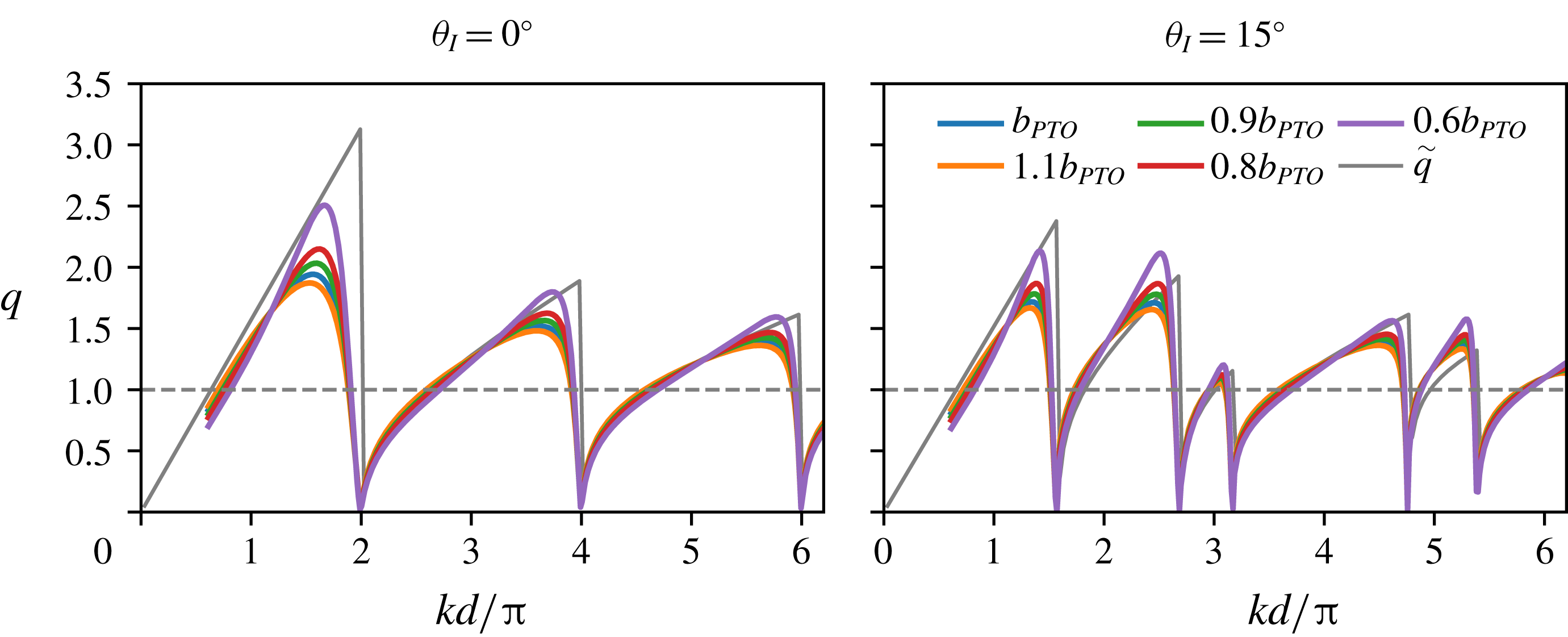
Transmission $|\unicode[STIX]{x1D6FF}_{m0}+A_{m}^{+}|$ (thick line) and reflection $|A_{m}^{-}|$ (thin line) amplitudes for a single-row truncated-vertical-cylinder periodic array of periodicity $d/2a=3.0$ , for $\unicode[STIX]{x1D703}_{I}=0^{\circ }$ , $30^{\circ }$ ( $\unicode[STIX]{x1D6FF}_{m0}$ is Kronecker delta). (a,d) Energy-extracting buoys. (b) Freely oscillating buoys. (c) Fixed buoys. Note that $A_{1}^{\pm }$ is hidden below $A_{-1}^{\pm }$ for $\unicode[STIX]{x1D703}_{I}=0^{\circ }$ .

The amplitudes of transmission and reflection coefficients $|A_{m}^{\pm }|$ for $d/2a=3.0$ array for $\unicode[STIX]{x1D703}_{I}=0^{\circ }$ and $\unicode[STIX]{x1D703}_{I}=30^{\circ }$ are shown in figure 12. We compare the performance of arrays consisting of energy-extracting, freely oscillating or fixed bodies as a function of wavenumber $kd$ . (Note that we plot the combined amplitude $|1+A_{0}^{+}|$ of the incident wave and the zeroth transmitted mode.) In general, when a new mode appears, there are abrupt changes in the amplitudes of other modes, as discussed in § 2. All the variations in mode amplitudes satisfy the energy conservation equation (4.11). The body-resonant wavenumber $k_{r}d$ is below the first Rayleigh wavenumber $(kd)_{1}^{cr}$ for normal incidence. For the WEC array at normal incidence, figure 12(a), the amplitudes of the modes $|A_{0}^{\pm }|$ achieve extremes near $k_{r}d$ , which is accompanied by a maximum of array gain $q$ (cf. figure 8 c). This maximum in $q$ is achieved by extracting a significant energy from both the transmitted $A_{0}^{+}$ and the reflected mode $A_{0}^{-}$ , as the comparison with the freely oscillating array shows (figure 12 b). For non-normal incidence, $k_{r}d$ falls between $(kd)_{1}^{cr}$ and $(kd)_{2}^{cr}$ , so there are additional modes present in the far field that radiate energy away from that array (figure 12 d). None of these modes, however, exhibits an extreme at $k_{r}d$ , and neither does $q$ (not shown). Note that for non-normal incidence the modes are not symmetric with respect to the array normal ( $x$ axis), so $A_{m}^{\pm }\neq A_{-m}^{\pm }$ and both are visible in figure 12(d). For wavenumbers much larger than $k_{r}d$ , the body motion becomes small (cf. figure 7 b), so the mode amplitudes are virtually identical between the energy-extracting, freely oscillating and fixed-body arrays. This is true for both normal and non-normal incidence.

It is interesting to note that the freely oscillating array at wavenumber $kd_{FR}$ (close to $k_{r}d$ ) behaves as a perfect reflector – the transmitted mode amplitude $|1+A_{0}^{+}|$ drops sharply to zero, and the reflected mode amplitude $|A_{0}^{-}|$ becomes one (figure 12 b). This is solely due to the body motion and not due to some underlying array resonance as the comparison with the periodic array of identical configuration with fixed bodies (figure 12 c reveals no distinguishable features present around $kd_{FR}$ ). For perfect reflection by single-row periodic arrays of heaving bodies, $kd_{FR}$ has to be below $(kd)_{-1}^{cr}$ in order for only one transmitted and reflected mode to be present, figure 13. If more modes are present, the one-degree-of-freedom motion cannot produce the wave field that would simultaneously cancel energy radiation in more than one direction, thus destroying the perfect reflection. The exact value of $kd_{FR}$ depends on periodicity $d$ and the incident angle $\unicode[STIX]{x1D703}_{I}$ , figure 14. The reflected mode amplitude $|A_{0}^{-}|$ as a function of $d$ for a given wavenumber $k_{r}a$ and incident angles $\unicode[STIX]{x1D703}_{I}=0^{\circ }$ and $15^{\circ }$ is shown in figure 14(a). The amplitude $|A_{0}^{-}|$ attains 1 at a single wavenumber $kd_{FR}$ , for both incident angles. For normal incidence, $kd_{FR}$ is only slightly larger than $k_{r}d$ for the $d/2a=3.0$ array, as expected from figure 12(b). With an increase in $\unicode[STIX]{x1D703}_{I}$ , $kd_{FR}$ is reduced. The dependency of $kd_{FR}$ on $d$ is shown in figure 14(b). The $kd_{FR}$ values monotonically increase as a function of $d/2a$ until reaching $(kd)_{-1}^{cr}$ for a given  $\unicode[STIX]{x1D703}_{I}$ , beyond which there are no perfect reflections. Correspondingly, $ka_{FR}$ values monotonically decrease from ${\sim}1.2$ to ${\sim}0.7$ . We note that the geometry of this heaving body has not been optimized to achieve the perfect reflection, indicating that this phenomenon is present for more general class of bodies. We confirmed this by conducting numerical simulations (not shown here) on heaving vertical cylinders of different shapes ( $a/h=0.5$ , $H/h=0.1$ ; $a/h=0.1$ , $H/h=0.1$ ) and found that perfect reflection is present at wavenumbers below $(kd)_{-1}^{cr}$ for those geometries as well.

Figure 13.

Contour plot of the reflected mode amplitude $|A_{0}^{-}|$ for a single-row periodic array of freely oscillating truncated vertical cylinders (no energy extraction), as a function of wavenumbers $kd\sin \unicode[STIX]{x1D703}_{I}$ and $kd$ , for $d/2a=2.0$ and 3.0.

Figure 14.

(a) The reflected mode amplitude $|A_{0}^{-}|$ for two different incident angles as a function of periodicity $d$ (at body-resonant wavenumber $k_{r}a$ ). Thin vertical dashed lines mark corresponding $(kd)_{-1}^{cr}$ ; thick vertical dashed red line marks $d/2a=3.0$ array. (b) Wavenumber $kd_{FR}$ (left $y$ -axis, dots) and $ka_{FR}$ (right $y$ -axis, dashed line) at which full reflection occurs as a function of spacing  $d$ , for two different incident angles. Horizontal lines in matching colour mark corresponding $(kd)_{-1}^{cr}$ ; thick red dashed horizontal line marks $k_{r}a$ .

Figure 15.

Free-surface amplitude $|\unicode[STIX]{x1D702}|$ contours for a single-body periodic array of truncated vertical cylinders of periodicity $d/2a=3.0$ . Waves are incident from the left. (a)  $kd=1.67\unicode[STIX]{x03C0}$ ( $ka=k_{r}a$ ), freely oscillating. (b)  $kd=1.67\unicode[STIX]{x03C0}$ ( $ka=k_{r}a$ ). (c)  $kd=2.01\unicode[STIX]{x03C0}$ ( $ka=1.05$ ). (d)  $kd=3.72\unicode[STIX]{x03C0}$ ( $ka=1.95$ ). (e)  $kd=2.01\unicode[STIX]{x03C0}$ ( $ka=1.05$ ). The body colour corresponds to the heave amplitude (lower colour bar).

The free-surface amplitude $|\unicode[STIX]{x1D702}|$ for the $d/2a=3.0$ array at specific wavenumbers and incident angles (marked in figure 12) is shown in figure 15. The effect of perfect reflection is demonstrated in figure 15(a), where freely oscillating bodies at body-resonant wavenumber $k_{r}a$ exhibit large heaving motion and almost completely reduce the free-surface amplitude behind the array ( $|\unicode[STIX]{x1D702}|\approx 0$ ). In front, $|\unicode[STIX]{x1D702}|$ is modulated with an increased amplitude between the nodes, as required by energy conservation. When energy extraction is present at the same wavenumber, figure 15(b), the bodies still perform large motions (significant energy extraction), but the array no longer acts like a perfect reflector ( $|\unicode[STIX]{x1D702}|>0$ behind the array). At a wavenumber just above $(kd)_{1}^{cr}$ , figure 15(c), a new mode of relatively large amplitude has just emerged and is propagating almost perpendicular to the incident wave, causing a significant modulation of the surface amplitude. The bodies are located in the low value troughs of the free-surface amplitude, resulting in almost zero $|X|$ and  $q$ . At $kd=3.72\unicode[STIX]{x03C0}$ , figure 15(d), which is still between $(kd)_{1}^{cr}$ and $(kd)_{2}^{cr}$ , $|1+A_{0}^{+}|\approx 1$ and the rest of the modes are almost zero (cf. figure 12), so the array minimally disturbs the free surface in the far field. Close to the array, however, the surface modulation is significant. The body motion amplitude $|X|$ in figure 15(c,d) is small, but for different reasons. In figure 15(c), the small $|X|$ is caused by a Rayleigh resonance, and it would be significantly larger if the wavenumber were slightly different. In figure 15(d), on the other hand, the small $|X|$ is caused by the fact that the wavenumber $ka$ is much larger than $k_{r}a$ , so the isolated-body amplitude is very small to start with and a small variation in $ka$ would not change $|X|$ significantly. For a non-normal incidence ( $\unicode[STIX]{x1D703}_{I}=30^{\circ }$ ) case, figure 15(e), the bodies exhibit large motion amplitudes, corresponding to large energy extraction ( $q=1.77$ ). The wide bands of nearly zero amplitude behind the array are a good indication of that.

Figure 16.

Array gain $q$ for a three-row periodic array of truncated vertical cylinders at resonant wavenumber $k_{r}a$ (a,b) and super-resonant wavenumber $k_{sr}a$ (c,d) as a function of row spacing $d_{x}$ and periodicity  $d$ . Each column corresponds to one incident angle  $\unicode[STIX]{x1D703}_{I}$ . Only the values for array configurations that satisfy the domain constraint $(N-1)d_{x}\leqslant d$ are plotted. Bragg resonances are marked by green vertical dashed lines; Rayleigh critical conditions are marked by magenta horizontal dashed lines. For comparison, point-absorber Laue-resonance lines based on (3.6) are marked by thin green lines.

6 Energy extraction by multi-row periodic arrays

One of the advantages of the multiple-scattering method presented in § 4 is that it is applicable to periodic WEC arrays of closely spaced sub-arrays of general, not necessarily identical bodies. We apply the method here to study the effect of the periodicity $d$ and row spacing $d_{x}$ on the array performance of rectangular periodic arrays with $N=3$ rows. For simplicity, we focus on arrays of identical truncated vertical cylinders, having the same shape and PTO characteristic as in § 5; the extraction rate $b_{PTO}$ is kept constant and equal for all the bodies in the array. This choice of $b_{PTO}$ values provides for an insightful study of the phenomena occurring in general (not just optimal) WEC arrays, with a simply defined $b_{PTO}$ distribution.

The array gain $q$ as a function of periodicity $d$ and row spacing $d_{x}$ for resonant and super-resonant wavenumbers ( $k_{r}a$ , $k_{sr}a$ ) and two incident angles ( $\unicode[STIX]{x1D703}_{I}=0^{\circ }$ , $15^{\circ }$ ) is shown in figure 16. To avoid the slow convergence of the periodicity matrix $\unicode[STIX]{x1D64C}$ discussed in § 4, we consider here only array configurations that satisfy the domain constraint $(N-1)d_{x}\leqslant d$ . The overall structure of $q$ resembles that of $\tilde{q}$ (cf. figure 3). The decrease in $q$ due to Rayleigh resonances and Bragg resonances are present at all wavenumbers and incident angles, confirming that these phenomena are an inherent feature of lattice-like periodic WEC systems, and not only of the point-absorber ones. Laue-resonance lines for the finite-body periodic arrays are, in general, slightly perturbed from those given by (3.6) due to the small phase shifts in the scattered modes relative to those for point-absorber arrays. For the sake of comparison with the point-absorber arrays, we plot the Laue resonance lines based on (3.6). We find that the regions of lower $q$ in general align well with the point-absorber Laue-resonance lines; the instances where these Laue-resonance lines cross the areas of high $q$ indicate that a larger phase shift in the scattered modes is present. The decrease in $q$ due to Laue resonances is more obvious for larger wavenumbers ( $k_{sr}a$ ) where Laue resonances are denser. Overall, $q$ obtains maximum values of 1.98 and 3.72 at $\unicode[STIX]{x1D703}_{I}=0^{\circ }$ for $k_{r}a$ and $k_{sr}a$ , respectively, and 1.66 and 2.28 for $\unicode[STIX]{x1D703}_{I}=15^{\circ }$ . Further increases in $q$ would be possible if the PTOs in a given array configuration were optimally tuned (cf. figure 11) for a specific wavenumber ( $k_{r}a$ or any other). In that case, $b_{PTO}$ of each body in the sub-array would have a different optimal value in general.

The comparison of the array gain $q$ at the body-resonant wavenumber $k_{r}a$ with the array gain $\tilde{q}$ for point-absorber arrays of equivalent configuration in equal-amplitude motion as a function of row spacing $d_{x}$ is shown in figure 17. Despite the absence of the equal-motion constraint for the truncated-cylinder WEC arrays, $q$ at $k_{r}a$ in general follows the behaviour of  $\tilde{q}$ , but it is even greater than $\tilde{q}$ within some intervals. The high values of $q$ in this case are not a result of the sub-optimal performance of the isolated body (extracted power by an isolated body at resonance is equivalent to that of an optimal point absorber), but are gains caused directly by favourable array interactions. The intervals where $q>\tilde{q}$ indicate the configurations for which the equal-amplitude motion of periodic point-absorber arrays is clearly sub-optimal because periodic arrays of non-optimized WECs (in terms of $b_{PTO}$ , shape) are performing better than the point-absorber arrays of identical configuration.

Figure 17.

Comparison of array gain $q$ for three-row truncated-cylinder periodic WEC arrays at resonance wavenumber $k_{r}a$ (dashed lines) with array gain $\tilde{q}$ for point-absorber arrays of equivalent configuration in equal-amplitude motion (solid lines), as a function of row spacing  $d_{x}$ . The results are plotted only for the range where the domain constraint $(N-1)d_{x}\leqslant d$ is satisfied. Vertical dashed lines denote Bragg resonances.

The light-cone plot of $q$ for two different array configurations, figure 18, reveals the detailed dependence of $q$ on $kd$ and  $\unicode[STIX]{x1D703}_{I}$ . The overall structure resembles that of an isolated body (cf. figure 9), with additional troughs in $q$ due to Bragg and Laue resonances. The Laue-resonance lines for point-absorber arrays (i.e. based on (3.6)) are plotted for comparison. Away from Bragg and Laue resonances high gains are attainable, especially for super-resonant wavenumbers (e.g. for $\unicode[STIX]{x1D703}_{I}=24^{\circ }$ , $\max q=6.08$ at $kd=5.03\unicode[STIX]{x03C0}$ ; for $\unicode[STIX]{x1D703}_{I}=47^{\circ }$ , $\max q=5.98$ at $kd=4.34\unicode[STIX]{x03C0}$ ).

Figure 18.

Light-cone plot of array gain $q$ for two different three-row periodic arrays of truncated vertical cylinders. Rayleigh critical conditions marked by dashed white lines, Bragg resonances by thick magenta lines, Laue resonances based on (3.6) by thin, dashed magenta lines and the body-resonant wavenumber by a dashed horizontal cyan line.

The array gain $q$ for a range of wavenumbers and periodicities in arrays of two different aspect ratios $d_{x}/d=0.45$ , 0.495, is plotted in figure 19. For aspect ratios $d_{x}/d\lesssim 0.5$ , the structure of $q$ is similar to that of $d_{x}/d=0.45$ . Compared to single-row performance (figure 8), $q$ still preserves the band-like structure determined by Rayleigh wavenumbers, but it is more intricate due to the presence of Bragg and Laue resonances. Higher values of $q$ still occur for larger $ka$ values (e.g. for $d_{x}/d=0.45$ configurations at $\unicode[STIX]{x1D703}_{I}=0^{\circ }$ , $\max q=8.60$ occurs for $d/2a=4.85$ and $kd=8.50\unicode[STIX]{x03C0}$ ( $ka=2.75$ )). For $ka<k_{r}a$ , $q\approx 1$ , which indicates that limited gains, in general, are possible in the sub-resonant regime; this behaviour is also similar to that found in single-row periodic arrays (cf. figure 8).

For configurations with the $d_{x}/d\approx 0.5$ aspect ratio, however, we find new features that cannot be attributed to the Rayleigh, Bragg or Laue resonances identified so far. These new features appear as sharp increases in $q$ that intersect the constant-wavenumber lines at an oblique angle. Consequently, they appear as narrow-banded features in the $kd$ -space for a given array configuration. These are, in fact, Fano features we discussed in § 2 and are the signatures of Rayleigh–Bloch waves. The striking feature of these Rayleigh–Bloch waves is that they are excited by the incident wave, i.e. they are embedded in the continuous spectrum, and their effect is easily recognizable in the response. Since these waves appear in a system where bodies are inherently moving, we borrow the terminology from McIver & McIver (Reference McIver and McIver2007) and refer to them as motion-trapped Rayleigh–Bloch waves. Note that these Rayleigh–Bloch waves are absent in the response of point-absorber arrays studied in § 3, including for the array configurations identical to those represented in figure 19. This stems from the fact that the phenomenon of Rayleigh–Bloch waves is inherently related to finite-size bodies and their interaction with the wave field.

Figure 19.

Contour plot of array gain $q$ of a three-row truncated-vertical-cylinder periodic array with aspect ratios $d_{x}/d=0.45$ (a,b) and $d_{x}/d=0.495$ (c,d). The yellow dashed line denotes the body-resonant wavenumber $k_{r}a$ ; green dashed line the super-resonant wavenumber $k_{sr}a$ . The contours are computed for wavenumbers $ka<3.0$ (cf. figure 7 c). The contour colour range is cropped to allow for a better resolution at $q$ -values of interest (around 1).

In order to study the structure and the sensitivity of the Rayleigh–Bloch waves, in the following we focus on three periodic arrays that appear to support Rayleigh–Bloch waves, but of slightly different configurations: configuration I with periodicity $d/2a=5.14$ and row spacing $d_{x}/d=0.48$ , configuration II with $d/2a=5.19$ and $d_{x}/d=0.50$ and configuration III with $d/2a=5.20$ and $d_{x}/d=0.50$ . The minor differences in periodicity and row spacing between these configurations provide a good basis for the sensitivity analysis of trapped waves with respect to configuration perturbations.

The array gain $q$ for configurations I, II and III as functions of wavenumber $kd$ are shown in figure 20. While all three configurations exhibit very similar behaviour for the most of the $kd$ range for $\unicode[STIX]{x1D703}_{I}=0^{\circ }$ , figure 20(a), configurations II and III exhibit sharp, narrow-bandwidth spikes – Fano features – at distinct wavenumbers $kd^{RB}$ . Both configurations exhibit two Fano features in the plotted interval, one occurring at $kd^{RB}$ below the Rayleigh wavelength $(kd)_{1}^{cr}$ , and one just above it. The first wavenumbers $kd^{RB}$ at which Rayleigh–Bloch waves occur are noticeably different between the two configurations, as are the magnitudes of Fano features, which indicates high sensitivity to perturbations in periodicity. Note that the orientations of the two Fano features for configuration II are different – the first exhibits a small decrease in $q$ followed by a sharp jump, while the second is preceded by an increase in $q$ followed by a sharp drop. Comparison of $q$ for configuration II at $\unicode[STIX]{x1D703}_{I}=0^{\circ }$ and $\unicode[STIX]{x1D703}_{I}=1^{\circ }$ , figure 20(b), reveals that the presence of Rayleigh–Bloch waves is very sensitive to angular perturbations. While for the most of the plotted $kd$ range the two lines are virtually indistinguishable, $q(\unicode[STIX]{x1D703}_{I}=1^{\circ })$ exhibits no significant Fano features despite only a minor variation in incident angle. Rayleigh–Bloch waves are not limited to normal incidence, however. Array gain $q$ for configuration I at specific non-normal incidence angles is shown in figure 20(c). Fano features below the lowest Rayleigh wavenumber $(kd)_{-1}^{cr}$ are present for all plotted incident angles. In the same way as in figure 20(b), a slight variation in $\unicode[STIX]{x1D703}_{I}$ will destroy the Rayleigh–Bloch waves.

While the presence of embedded Rayleigh–Bloch waves is highly sensitive to perturbations of $k$ and $\unicode[STIX]{x1D703}_{I}$ , based on figure 19 we can argue that a large range of three-body rectangular periodic arrays with $d_{x}/d\approx 0.5$ support one or more embedded Rayleigh–Bloch waves at some $kd$ and  $\unicode[STIX]{x1D703}_{I}$ . Changing the periodicity (while keeping the same aspect ratio $d_{x}/d$ ) merely changes $k$ and $\unicode[STIX]{x1D703}_{I}$ at which Rayleigh–Bloch waves occur.

Figure 20.

Array gain $q$ as a function of wavenumber $kd$ for three-row periodic arrays of truncated vertical cylinders. (a) Three different array configurations at $\unicode[STIX]{x1D703}_{I}=0^{\circ }$ ; (b) configuration II at $\unicode[STIX]{x1D703}_{I}=0^{\circ },1^{\circ }$ ; (c) non-normal incidence for configuration I. Rayleigh wavenumbers $(kd)_{-1}^{cr}$ are marked by thin vertical lines (in corresponding colour in (c)); the body-resonant wavenumber is marked in dashed red vertical line. Arrows in (a) mark the cases that are plotted in figure 23.

The effect of trapped waves on power extraction effectiveness of each body – the percentage of power $p_{i}=P_{i}/P_{a}$ extracted by body $i$ – is shown in figure 21. For configuration I, all the bodies are almost equally effective in energy extraction for wavenumbers below the first Rayleigh wavenumber. Above the first Rayleigh wavenumber, such balance is no longer present and the variation of $p_{i}$ with $kd$ is different for each body, usually with all three bodies extracting different amounts of energy. At the resonant wavenumber $k_{r}a$ , all the values of $p_{i}$ are again almost equal. For configuration II, on the other hand, the sharp Fano features are present again – $p_{i}$ at trapped-wave wavenumbers exhibits an abrupt increase or decrease, and it is most prominent for bodies 1 and 2. Note that the Fano features are also observed in the motion response (not shown). The heave amplitude $|X_{i}|$ of each body can be calculated from (2.8) and (2.9) as $|X_{i}|=|X|\sqrt{Nqp_{i}}$ , where $|X|$ is the heave amplitude of an isolated body, figure 7(b).

Figure 21.

Comparison of the percentage of extracted power $p_{i}$ by each of the bodies in a three-row periodic array of truncated vertical cylinders, for two different array configurations at $\unicode[STIX]{x1D703}_{I}=0^{\circ }$ . Rayleigh wavenumbers are marked by grey vertical lines; the body-resonant wavenumber is marked by dashed red vertical lines.

Comparison of the amplitudes of the zeroth scattering modes $|A_{0}^{\pm }|$ for the three configurations is shown in figure 22. At the first trapped-wave wavenumber $kd^{RB}$ , $|A_{0}^{+}|$ for configurations II and III exhibits a sharp decrease, matched by an equally sharp increase in $|A_{0}^{-}|$ , as required for energy conservation. The Fano features at the second trapped wavenumber are somewhat less pronounced. Interestingly, the Fano features persist even for same-configuration arrays of freely oscillating bodies (no power extraction) and of fixed bodies, although they are less pronounced in the latter case. This indicates that WEC arrays that support motion-trapped Rayleigh–Bloch waves also support trapped waves in arrays of fixed bodies at the same, or nearly the same, wavenumbers. The trapped waves that occur in fixed structures are called sloshing trapped waves; they have been observed, for example, in isolated three-dimensional bodies with a central moonpool (McIver & McIver Reference McIver and McIver2007).

Note that Fano features in $|A_{0}^{\pm }|$ for these three-row periodic arrays are different from the narrow-banded, total reflection features in $|A_{0}^{\pm }|$ occurring for single-row periodic arrays (figure 12). In single-row periodic arrays, the narrow-banded feature is only present for arrays with freely oscillating bodies; it is smoothed out when the bodies are extracting energy, and it is absent for fixed bodies. Furthermore, the free-surface elevation amplitude $|\unicode[STIX]{x1D702}|$ is much lower in the perfect reflection case (figure 15 a), compared to $|\unicode[STIX]{x1D702}|$ at trapped-wave wavenumbers (figure 23 a,c,d).

Figure 22.

The transmitted $|A_{0}^{+}|$ (thick lines) and reflected mode $|A_{0}^{-}|$ (thin lines) amplitudes for three-row periodic arrays of truncated vertical cylinders at $\unicode[STIX]{x1D703}_{I}=0^{\circ }$ incidence. (a) Energy-extracting bodies; (b) freely oscillating bodies; (c) fixed bodies. Rayleigh wavenumber (indistinguishable difference in $(kd)_{1}^{cr}$ between the three configurations) is marked by a grey vertical line; body-resonant wavenumber by a dashed red line.

The amplitude of the free-surface elevation $|\unicode[STIX]{x1D702}|$ for the three configurations at specific wavenumbers for $\unicode[STIX]{x1D703}_{I}=0^{\circ }$ is shown in figure 23. The free-surface amplitude around the configuration-II array at its first trapped-wave wavenumber (figure 23 a) shows very high elevation ( $|\unicode[STIX]{x1D702}|\sim 10.7$ ) around bodies 1 and 3. Body 1 extracts most of the energy (and undergoes largest heave motions $|X_{1}|$ ), while body 2 extracts almost no energy at all (i.e. is barely moving). The high $q$ achieved in this case is manifested by a significant decrease in $|\unicode[STIX]{x1D702}|$ everywhere behind the array. For configuration II, we also consider two distinct wavenumbers around the second trapped-wave wavenumber, one from each side of the (asymmetric) jump: $kd=2.08\unicode[STIX]{x03C0}$ before the jump, corresponding to the higher $q$ value (figure 23 b), and $kd=2.10\unicode[STIX]{x03C0}$ after the jump, corresponding to the lower $q$ value (figure 23 c). In this case, high- $q$ values do not correspond to high- $|\unicode[STIX]{x1D702}|$ values – $|\unicode[STIX]{x1D702}|$ is higher for the low- $q$ case. The high elevation $|\unicode[STIX]{x1D702}|$ occurs around bodies 1 and 3, but also between the bodies in the second row. Furthermore, the distribution of power among the bodies is different between the two wavenumbers: in the high- $q$ case the middle body extracts the most power, while in the low- $q$ case, the middle body is barely moving. Overall, the performance of the array is starkly different across the Fano feature.

The free-surface amplitude at the first and second trapped-wave wavenumbers for configuration III (figure 23 d,e) follows a similar pattern to that of configuration II. For both trapped-wave wavenumbers, the middle body extracts almost no energy (i.e. is barely moving), with the highest elevations occurring at bodies 1 and 3. At the body-resonant wavenumber $k_{r}a$ , all the bodies in configuration I extract energy equally (figure 23 f). The free-surface elevation behind the array is significantly reduced, which, together with a relatively mild modulation of the free surface in front, indicates efficient energy extraction and a high $q$ value.

Figure 23.

Free-surface amplitude $|\unicode[STIX]{x1D702}|$ contours for three slightly perturbed configurations of three-row truncated-vertical-cylinder periodic arrays at specific wavenumbers, for $\unicode[STIX]{x1D703}_{I}=0^{\circ }$ . (a) Configuration II, $kd=1.45\unicode[STIX]{x03C0}$ . (b) Configuration II, $kd=2.08\unicode[STIX]{x03C0}$ . (c) Configuration II, $kd=2.10\unicode[STIX]{x03C0}$ . (d) Configuration III, $kd=1.69\unicode[STIX]{x03C0}$ . (e) Configuration III, $kd=2.05\unicode[STIX]{x03C0}$ . (f) Configuration I, $kd=2.86\unicode[STIX]{x03C0}$ . The body colour denotes the power extraction percentage $p_{i}$ of each body (according to the right colour bar).

The amplitude of free-surface elevation along the $x$ and $y$ axes for configurations I and II is shown in figure 24. For configuration I, the free surface is shown for the body-resonant wavenumber $k_{r}a$ where there is significant energy extraction. The free-surface amplitude behind the array exhibits much longer modulation compared to that in front. The mean amplitude along a row, i.e. along $x=0,d_{x},2d_{x}$ , is generally decreasing for larger  $x$ . For configuration II, $|\unicode[STIX]{x1D702}|$ is shown for $kd=1.45\unicode[STIX]{x03C0}$ , which corresponds to the first trapped-wave wavenumber (cf. figure 23 a), and for $kd=2.08\unicode[STIX]{x03C0}$ and $2.10\unicode[STIX]{x03C0}$ , corresponding to wavenumbers surrounding the second trapped-wave wavenumber (cf. figure 23 b,c). High free-surface elevations at the cylinder surface are visible for the first trapped-wave wavenumber, as well as the high elevation in between the bodies in the second row at the third wavenumber ( $kd=2.10\unicode[STIX]{x03C0}$ ).

Figure 24.

Free-surface amplitude $|\unicode[STIX]{x1D702}|$ for two slightly perturbed configurations of three-row truncated-vertical-cylinder periodic arrays at specific wavenumbers, for $\unicode[STIX]{x1D703}_{I}=0^{\circ }$ . The amplitude is plotted for $y=0$ (a,c) and at three different $x=\text{const.}$ (b,d). Grey vertical bars in both views denote the locations of the bodies.

We remark on the numerical convergence of the results in this section. As in § 5, the results presented in this section generally converge to $O(1\,\%)$ . The exceptions are the values obtained for wavenumbers close to $kd^{RB}$ , where the qualitative conclusions about the Rayleigh–Bloch waves remain valid as the number of modes in partial wave decomposition is increased, although the quantitative values may be affected. We also note that the large free-surface elevations due to Rayleigh–Bloch waves indicate that the linear wave theory is not strictly valid at those wavenumbers because the small-wave-steepness assumption is violated. For an accurate analysis of array performance at trapped-wave wavenumbers, one should conduct nonlinear computations based on the models that include nonlinear wave dynamics and wave–body interactions.

Finally, we remark that while we focus here on the three-row periodic WEC arrays only, we have performed similar computations (and analyses) for two- and four-row periodic arrays (not presented). The results for these configurations show a similar character as those for the three-row arrays presented here, including the decrease in the array gain at Rayleigh, Bragg and Laue resonances, as well as the presence of embedded motion-trapped Rayleigh–Bloch waves for configurations with $d_{x}/d\approx 1/(N-1)$ . Furthermore, our choice of the body shape is purely arbitrary and not special in any way. This indicates that these findings should also be valid for arrays consisting of bodies of general (axisymmetric) shape.