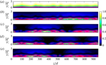
1. Introduction
Thirty-five years ago, Morkovin (Reference Morkovin1979) summarised observations of streamwise vorticity in boundary layers and the absence of a causative condition, although an empirical link to wind-tunnel settling chamber screens had been established. Experiments on nominally two-dimensional flows in wind tunnels cannot be assumed to be two-dimensional. Streamwise vorticity generates spanwise variation (streaks) that can significantly alter the boundary-layer properties and stability characteristics. At elevated free-stream turbulence (FST) levels, the streaks are called Klebanoff streaks and transition to turbulence is often via a bypass mechanism (see Zaki Reference Zaki2013; Goldstein Reference Goldstein2014 for recent reviews). However, even at low FST levels, significant spanwise variation and streaks can be observed in some experiments.
1.1. Observations of boundary-layer spanwise variation
Spanwise boundary-layer variation can manifest in differing ways. The spanwise spacing of Görtler vortices has been linked to the free stream (Swearingen & Blackwelder Reference Swearingen and Blackwelder1987), while early boundary-layer transition studies noted significant spanwise variation (Klebanoff, Tidstrom & Sargent Reference Klebanoff, Tidstrom and Sargent1961). Advances have shown this to be a secondary instability of the Tollmien–Schlichting (TS) wave (Herbert Reference Herbert1988), although weak streaks can affect the spanwise scale and secondary instability growth rate, delaying or promoting transition (Liu, Zaki & Durbin Reference Liu, Zaki and Durbin2008b ). The simulations of Schlatter et al. (Reference Schlatter, Deusebio, de Lange and Brandt2011) provide a graphical demonstration.
Klebanoff streaks, often associated with elevated FST levels (Klebanoff Reference Klebanoff1971; Kendall Reference Kendall1985; Westin et al. Reference Westin, Boiko, Klingmann, Kozlov and Alfredsson1994; Kendall Reference Kendall1998; Watmuff Reference Watmuff1998; Matsubara & Alfredsson Reference Matsubara and Alfredsson2001; Fransson, Matsubara & Alfredsson Reference Fransson, Matsubara and Alfredsson2005b ; Nolan & Walsh Reference Nolan and Walsh2012), are a form of spanwise variation that can influence transition involving TS waves. Boiko et al. (Reference Boiko, Westin, Klingmann, Kozlov and Alfredsson1994) observed forced TS wave growth to be reduced by Klebanoff streaks, although transition shifted upstream. However, Watmuff (Reference Watmuff1998) found that flow quality improvements to reduce Klebanoff streaks shifted the natural transition upstream, similar to Arnal & Juillen (Reference Arnal and Juillen1978), who increased the FST and found a downstream transition shift on a body of revolution. However, Kendall (Reference Kendall1991) observed increased TS-wave-packet growth rates in the presence of Klebanoff streaks.
Computations (Cossu & Brandt Reference Cossu and Brandt2002) and stability theory (Cossu & Brandt Reference Cossu and Brandt2004; Bagheri & Hanifi Reference Bagheri and Hanifi2007) have shown that the steady optimal streak (Andersson, Berggren & Henningson Reference Andersson, Berggren and Henningson1999; Luchini Reference Luchini2000) reduces TS-wave growth rates. Streaks forced by roughness elements (Fransson et al. Reference Fransson, Brandt, Talamelli and Cossu2005a ; Gürün Reference Gürün2006) or miniature vortex generators (Fransson & Talamelli Reference Fransson and Talamelli2012) have also shown reduced TS-wave growth, and sometimes transition delay (Fransson et al. Reference Fransson, Talamelli, Brandt and Cossu2006; Shahinfar et al. Reference Shahinfar, Sattarzadeh, Fransson and Talamelli2012; Shahinfar, Sattarzadeh & Fransson Reference Shahinfar, Sattarzadeh and Fransson2014). However, both steady and unsteady streaks forced by a single Squire mode have been found to increase TS-wave growth (Vaughan & Zaki Reference Vaughan and Zaki2011), depending on streak amplitude, indicating that the forcing of the streak is an important consideration. Free-stream disturbances generated by wind-tunnel screens are known to force Klebanoff streaks, but the link is still tenuous. Klebanoff streak amplitude and the influence on transition have yet to be linked directly with measures of a screen.
Turbulent boundary layers are also affected by spanwise variation. Unexplained spanwise variation in both the tripped and non-tripped turbulent layers, generating a mixing flow, have been observed by Bell & Mehta (Reference Bell and Mehta1990). Dengel & Fernholz (Reference Dengel, Fernholz, Fernholz and Fiedler1989) found spanwise variation in the turbulent layer and showed direct linkage to the settling chamber screens by rotating them. Spanwise variation was considerably reduced by replacing the screen with one constructed from perforated metal.
1.2. Spanwise variation empirically linked to settling chamber screens
Wind-tunnel settling chamber screens and honeycombs are used to reduce FST levels and improve flow quality, yet many experimentalists identify them as directly influencing the test-section boundary layer. Bradshaw (Reference Bradshaw1965) studied a tripped, turbulent boundary layer on the test-section floor that exhibited spanwise variation of skin friction in excess of 10 %. The spanwise variation was dependent on the individual screen, its orientation and was repeatable when the open-area ratio was greater than 57 %. Decreasing the open-area ratio below 57 % produced a boundary layer with considerably increased spanwise variation. This was attributed to a spatial flow instability downstream of the screen called the coalescence of jets. The coalescence of jets is a local change of flow pattern that occurs downstream of low open-area ratio zithers. Requiring screens to have an open-area ratio greater than 57 % has become a guideline when selecting screens for wind tunnels.
Crow (Reference Crow1966), in response to the findings of Bradshaw (Reference Bradshaw1965), analytically investigated the effect of small, steady spanwise variations of transverse velocity above a laminar boundary layer. Small velocity variations could create spanwise variations in the boundary layer. Experiments by de Bray (Reference de Bray1967) confirmed the findings of Bradshaw (Reference Bradshaw1965). A high quality honeycomb was also observed to produce a more spanwise uniform boundary layer while locating the test-section plate on the wind-tunnel centreline could reduce the spanwise variation by 50 % compared to the wind-tunnel wall boundary layer. de Bray (Reference de Bray1967) concluded that immeasurable non-uniformities introduced by screens persist into the test section and affect the spanwise variation of the layer. He postulated that vortices of opposite rotation (apparently streamwise oriented) originate from adjacent openings in the screen and bundle together (coalesce) downstream.
Similarly, Patel (Reference Patel1964) observed reduced spanwise variation when using a honeycomb downstream of the settling chamber screens, although this configuration can increase FST levels (Mehta & Bradshaw Reference Mehta and Bradshaw1979). However, Scheiman & Brooks (Reference Scheiman and Brooks1981) found that a honeycomb upstream of a screen produced a greater reduction of turbulence levels. Patel (Reference Patel1964) also noted increased spanwise variation with dust accumulation on the screens, underscoring the sensitivity of the test-section layer to screen quality.
The widespread consensus is that jets coalesce downstream of the screen due to some ‘instability’ formed at low open-area ratios. From this instability, streamwise vortices form (de Bray Reference de Bray1967; Mehta & Bradshaw Reference Mehta and Bradshaw1979), which persist through the contraction and into the test-section layer. However, Mehta & Hoffmann (Reference Mehta and Hoffmann1987) found increased spanwise variation does not always correlate directly with an open-area ratio of 57 %. Two screens, both with an open-area ratio of 58.8 %, created spanwise skin-friction variation of 10 % and 18 %. They concluded the 57 % open-area ratio criteria is not sufficient to guarantee two-dimensionality of the test-section boundary layer. Mehta (Reference Mehta1985) also tested screens of varying materials and construction methods. Plastic screens were found to produce less spanwise variation relative to woven metal screens.
Increased spanwise variation of the test-section boundary layer can also be associated with increased FST levels. Klebanoff (Reference Klebanoff1971) elevated the FST level in a wind tunnel with grids constructed of rope that were placed upstream of the contraction. A low-frequency spanwise thickening and thinning of the layer was observed that grew with increasing FST levels (Klebanoff streaks). However, the measurements of Watmuff (Reference Watmuff1998) suggest the link between FST and Klebanoff streaks is not simple. Watmuff found that replacing and tensioning the settling chamber screens reduced the FST level from 0.12–0.08 %, but the Klebanoff streaks in the boundary layer (measured by
 $u_{rms}$
) decreased by a factor of three. The unsteadiness in the layer was not spanwise uniform but clustered into ‘clump’ regions that did not shift with time. The unsteadiness in the layer was reduced by a further factor of two by reordering the screens based on quality, as measured from laser scans, from least uniform (worst quality) to most uniform (best quality) downstream.
Westin et al. (Reference Westin, Boiko, Klingmann, Kozlov and Alfredsson1994) compiled published results of Klebanoff streak growth and found considerable differences, even when scaled with the FST level. However, the observed spacing of Klebanoff streaks generally shows a more reasonable agreement, approximately twice the boundary-layer thickness (
 ${\sim}2{\it\delta}_{99}$
). Matsubara & Alfredsson (Reference Matsubara and Alfredsson2001) observed the physical spacing of Klebanoff streaks to be independent of the mesh spacing used in the construction of a grid placed in the test section to elevate the FST levels, however streak spacing has been found to be dependent on the free-stream environment (Fransson & Alfredsson Reference Fransson and Alfredsson2003; Ovchinnikov, Choudhari & Piomelli Reference Ovchinnikov, Choudhari and Piomelli2008).
Swearingen & Blackwelder (Reference Swearingen and Blackwelder1986) found the ‘natural’ spacing of Görtler vortices to be sensitive to the settling chamber screens. The spacing was independent of the screen mesh length, test section width, distance of the last screen from the contraction and FST variation created by the removal of the honeycomb upstream of the screens. However, the spanwise pattern of Görtler vortices was stationary in time and strongly dependent on the downstream screen. Vertical cylinders oriented normal to the test-section leading edge, and placed in the tunnel contraction, were used to alter the screen wake. Cylinder spacing larger than the natural Görtler spacing did not substantially alter the spanwise pattern, but the cylinder wakes were clearly visible in the boundary layer as narrow regions superimposed on the ‘natural’ pattern. Reducing cylinder spacing created a near-periodic variation, approximating the cylinder spacing. The mechanism for the cylinder wake affecting the Görtler spacing was described as the creation of streamwise vorticity when the wakes intersect the leading edge and are stretched by the boundary layer. At elevated FST levels, travelling Görtler vortices can be important (Schrader, Brandt & Zaki Reference Schrader, Brandt and Zaki2011; Wu, Zhao & Luo Reference Wu, Zhao and Luo2011).
Unlike streaks and Görtler vortices, the growth of cross-flow vortices on swept wings does not appear to be sensitive to free-stream non-uniformity. Deyhle & Bippes (Reference Deyhle and Bippes1996) found no effect on cross-flow spacing when shifting screens to change the dominant free-stream wavelength. The cross-flow pattern shifted with movement of the body, indicating surface roughness was the dominant factor. However, cross-flow growth and transition is very sensitive to FST, and hence screens (see Hunt Reference Hunt2011).
All of these observations clearly link settling chamber screens with spanwise variation in the test-section boundary layer and establish screen open-area ratio and quality as causal factors without any satisfactory explanation. Stationary Klebanoff streaks and Görtler vortices, and differing spanwise skin friction measurements depending on test-section plate location, question any assumption of a homogeneous screen wake and FST across a wind-tunnel cross section.
1.3. Flow downstream of screens
The classical analysis of Taylor & Batchelor (Reference Taylor and Batchelor1949) considered the linear, inviscid flow of streamlines through a gauze (screen) where a pressure drop takes place. Classical analysis does not consider the details of the screen or honeycomb beyond the pressure drop and deflection coefficients (Laws & Livesey Reference Laws and Livesey1978). However, Scheiman & Brooks (Reference Scheiman and Brooks1981) found screens suppressed longitudinal turbulence better than the lateral component, while honeycombs did the opposite. They deduced the mechanism responsible is different, which cautions the use of simple theory to understand the effects of screens, honeycomb or other turbulence manipulators.
Classical analysis predicts a pressure drop coefficient of 2.76 will remove any mean streamwise flow non-uniformity. Decreasing screen open-area ratio will increase the pressure drop. Hancock (Reference Hancock1998) extended the analysis to multiple screens and found no series of screens can perfectly attenuate free-stream non-uniformity, although any series of screens can give significant attenuation if the sum of the pressure drops coefficients is greater than 2.5. Bradshaw (Reference Bradshaw1965) recommended screens should have a pressure drop coefficient less than 1.6 to avoid jet coalescence. This is significantly lower than the analysis of Taylor & Batchelor (Reference Taylor and Batchelor1949) indicates is required to achieve uniform flow. Schubauer, Spangenberg & Klebanoff (Reference Schubauer, Spangenberg and Klebanoff1950) and Bradshaw (Reference Bradshaw1965) have recommended a series of lower pressure drop screens be used to achieve a high pressure drop.
Morgan (Reference Morgan1960) summarises early work on the coalescence of jets behind screens and zithers of low open-area ratio. Important points are that the instability occurs for open-area ratios less than approximately 50 %, and that imperfections of the screen (quality) have been postulated as a possible cause. Earlier experimental work by Bohl (Reference Bohl1940) (the original work is in German and the current authors cannot directly review it. The review is based on the reading of Morgan (Reference Morgan1960) and Corrsin (Reference Corrsin1944)) studied the flow downstream of a zither constructed of sharp wooden slats and provided the first analytical treatment of the coalescence of jets. Stable flow (no coalescence of jets) was observed for an open-area ratio of 63 % and unstable flow (with coalescence of jets) for an open-area ratio of 50 %. An analytical analysis was provided but Corrsin (Reference Corrsin1944) has criticised it for unclear physical assumptions in the derivation, although the results show qualitative agreement with experiment. Observations of the coalescence of jets have shown the flow pattern can be either stable in time or variable, and that multiple jets can coalesce at very low open-area ratios (Cheng & Moretti Reference Cheng and Moretti1988; Le Gal et al. Reference Le Gal, Peschard, Chauve and Takeda1996).
Böttcher & Wedemeyer (Reference Böttcher and Wedemeyer1989) examined the steady wakes of screens and zithers as the sum of each individual wire’s wake, governed by the linear diffusion equation. It should be noted that the coalescence of jets is equivalent to the merging of wakes (Corrsin Reference Corrsin1944). The wake strength and wavelength of a zither was derived by considering each wire randomly perturbed from its position in a zither with perfect wire spacing. Direct comparison between theory and experiment was not possible as inputs to the wake strength formula had to be estimated. Their analysis offers the potential to relate screen quality to the downstream wake.
The wake turbulence of a screen is also affected by the open-area ratio and the coalescence of jets. Loehrke & Nagib (Reference Loehrke and Nagib1972) and Tan-Atichat, Nagib & Loehrke (Reference Tan-Atichat, Nagib and Loehrke1982) found the decay of turbulent energy downstream of a low open-area ratio (30 %) perforated plate was greatly reduced relative to plates with open-area ratios of 51 % and 58 %. They suggest the coalescence of jets may be responsible. Irregularities were also observed in the mean flow far downstream. Previously, Schubauer et al. (Reference Schubauer, Spangenberg and Klebanoff1950) had noted that low open-area ratio screens (high pressure drops) could produce abnormally large streamwise velocity fluctuations and less uniform mean flow, but the cause was not identified. Recent computations by Ertunç et al. (Reference Ertunç, Özyilmaz, Lienhart, Durst and Beronov2010) show turbulence downstream of a symmetric (perfect) screen is not homogeneous. If the screen has small non-uniformities in its construction (variation in wire position), then the mean flow is also non-homogeneous.
No satisfactory explanation exists for the coalescence of jets, nor does the traditional inviscid analysis of screens predict its appearance or effects. To the authors knowledge, there has been no direct observation of the coalescence of jets for a screen (as opposed to a zither) and all reports of increased spanwise variation attributed to this phenomena have not directly observed its occurrence. How the change in flow pattern at a screen, located upstream of a contraction which produces near uniform streamwise velocity mean-flow but increases spanwise variation of the test-section boundary layer, is not fully explained.
1.4. Creating the link to settling chamber screens
Explaining the creation of spanwise variation and streaks in the boundary layer requires understanding of how disturbances grow in the layer, the receptivity of disturbances, the evolution of the disturbance in the free stream from their source and the creation of the disturbances at a source (screen). Recent work has focused on streak growth via non-modal theories (Andersson et al. Reference Andersson, Berggren and Henningson1999; Luchini Reference Luchini2000; Schmid Reference Schmid2007) or transient/algebraic growth (Ellingsen & Palm Reference Ellingsen and Palm1975; Hultgren & Gustavsson Reference Hultgren and Gustavsson1981; Butler & Farrell Reference Butler and Farrell1992; Reddy, Schmid & Henningson Reference Reddy, Schmid and Henningson2008). Asymptotic analyses have linked Klebanoff streaks to FST (Leib, Wundrow & Goldstein Reference Leib, Wundrow and Goldstein1999; Wundrow & Goldstein Reference Wundrow and Goldstein2001; Ricco Reference Ricco2009; Ricco, Luo & Wu Reference Ricco, Luo and Wu2011) and highlighted the importance of free-stream anisotropy. Goldstein, Leib & Cowley (Reference Goldstein, Leib and Cowley1992) and Goldstein & Leib (Reference Goldstein and Leib1993) describe the receptivity of normal and streamwise vorticity that creates streaks, while the computations of Schrader et al. (Reference Schrader, Brandt, Mavriplis and Henningson2010) and Pook & Watmuff (Reference Pook and Watmuff2014) demonstrate the preference for the receptivity of streamwise vorticity.
Pook & Watmuff (Reference Pook and Watmuff2014) have also demonstrated how normal vorticity entering a wind-tunnel contraction can be tilted and stretched into significant streamwise vorticity at the exit, away from the wind-tunnel centreline. This is consistent with the observations by de Bray (Reference de Bray1967) of increased skin friction variation away from the wind-tunnel centreline, suggesting the tilting and stretching of normal vorticity in the contraction can be a significant mechanism in the generation of spanwise variation of the test-section boundary layer and Klebanoff streaks. Any analysis that attempts to link spanwise variation to settling chamber screens must consider the contraction. Streaks that link directly to a physical, free-stream disturbance from a defined source in a wind tunnel may be important for determining their effect on the boundary-layer stability and transition.
1.5. Overview
This paper will focus on streak generation in a ‘clean’ wind-tunnel facility where the boundary-layer spanwise variation is time invariant, e.g. Watmuff (Reference Watmuff1998) with FST
 ${\sim}0.1\,\%$
. The streaks, created by an imperfect zither located upstream of a contraction, will be weak and bypass transition would not be expected. Modelling a zither is less computationally expensive than a screen, and provides an initial step towards Morkovin’s call to link screens with the test-section boundary layer. The current work is strictly applicable to zithers with steady laminar wakes, however qualitative similarities with observations made from screens will be noted. The work is divided into the following sections:
-
(i) Section 2 examines the steady laminar wakes of an imperfect zither, extending the analysis of Böttcher & Wedemeyer (Reference Böttcher and Wedemeyer1989). Substantial variation of drag across a zither is shown to lead to a reduced wake decay rate, but this decay rate is not so easily realised.
-
(ii) Section 3 passes the wakes through a 5:1, two-dimensional contraction. This will create streamwise vorticity at the exit via tilting and stretching of normal vorticity.
-
(iii) Section 4 documents the streaks formed in the flat-plate boundary layer by the wake of streamwise vorticity.
-
(iv) Section 5 assesses the linear stability of the test-section streak base-flows.
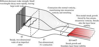
The contraction geometry, and the test-section leading edge shape and position, are the same as Watmuff (Reference Watmuff2006), Pook (Reference Pook2013), Pook & Watmuff (Reference Pook and Watmuff2014). An overview is provided in figure 1.
Overview of geometry and section breakdown.

2. The steady laminar wake of a zither
The (simplified) governing equation of a far wake is the linear diffusion equation (Böttcher & Wedemeyer Reference Böttcher and Wedemeyer1989; Batchelor Reference Batchelor2000),
 $$\begin{eqnarray}Uu_{x}={\it\nu}u_{zz},\end{eqnarray}$$
where
 $u=u(x,z)$
is the streamwise velocity of the wake,
 $U$
the uniform free-stream flow and
 ${\it\nu}$
is the fluid kinematic viscosity. Considering a spanwise (
 $z$
) periodic domain of width
 $L$
and a zither with
 $N$
wires, it can be shown that the solution to (2.1) is,
 $$\begin{eqnarray}u(x,z)=\mathop{\sum }_{k=-\infty }^{\infty }a_{k}\exp \left(\frac{2{\rm\pi}\text{i}kz}{L}\right)\exp (-4{\rm\pi}^{2}K^{2}\overline{x}),\end{eqnarray}$$
where
 $a_{k}$
are the unknown Fourier coefficients at the wake origin,
 $k$
is the integer wavenumber,
 $K$
is
 $k/N$
and
 $\overline{x}$
is a non-dimensional streamwise distance defined by,
 $$\begin{eqnarray}\overline{x}=\frac{x}{M}\frac{1}{Re_{M}},\end{eqnarray}$$
where
 $Re_{M}$
is the Reynolds number based on perfect zither wire spacing (
 $M$
). The wake energy is found as,
 $$\begin{eqnarray}\overline{u^{2}}=\frac{1}{L}\int _{0}^{L}(U-u)^{2}\,\text{d}z=\mathop{\sum }_{k=-\infty }^{\infty }|a_{k}|^{2}\exp (-8{\rm\pi}^{2}K^{2}\overline{x}),\end{eqnarray}$$
where the mean flow mode (
 $k=0$
) is not included in the summation. The value of a given Fourier coefficient in the downstream wake can be evaluated by multiplying it with,
 $$\begin{eqnarray}f=\exp (-4{\rm\pi}^{2}K^{2}\overline{x}).\end{eqnarray}$$
2.1. Summation of wakes
The wake of a zither will be considered as the summation of each individual wire’s wake. Unlike Böttcher & Wedemeyer (Reference Böttcher and Wedemeyer1989), each wire will be assumed to have an individual wake. Each wake is given by an unknown function,
 $W_{n}(z-z_{n})$
, where
 $z_{n}$
is the spanwise location of the
 $n$
th wire. Far downstream, the wavelengths are large in comparison to the wire spacing, as observed by Böttcher & Wedemeyer (Reference Böttcher and Wedemeyer1989). They argue that the wake function of a wire can be considered as a point source,
 $$\begin{eqnarray}\int W_{n}(z-z_{n})=q_{n}{\it\delta}(z-z_{n}),\end{eqnarray}$$
where
 ${\it\delta}(z-z_{n})$
is the Dirac function and
 $q_{n}$
is the source strength of the
 $n$
th wire. Assuming only a drag force acting on the wire (no lateral force component),
 $q_{n}$
is then related to the drag force (
 $D_{n}$
) by
 $D_{n}={\it\rho}Uq_{n}$
, where
 ${\it\rho}$
is density (Batchelor Reference Batchelor2000). Every wire in the zither is perturbed from its perfect position (
 $Mn$
), giving the position and source strength of the
 $n$
th wire as,
 $$\begin{eqnarray}z_{n}=M(n+{\it\delta}_{n}),\quad q_{n}=\overline{q}(1+{\it\epsilon}_{n}),\end{eqnarray}$$
where
 ${\it\delta}_{n}$
and
 ${\it\epsilon}_{n}$
are non-dimensional random variables with zero means and
 ${\it\delta}_{n}\ll M$
,
 ${\it\epsilon}_{n}\ll 1$
and
 $\overline{q}$
is the mean source strength. The Fourier coefficients of (2.2) are then,
 $$\begin{eqnarray}a_{k}=\frac{\overline{q}}{NM}\mathop{\sum }_{n=1}^{N}(2{\rm\pi}\text{i}K{\it\delta}_{n}+{\it\epsilon}_{n}-2{\rm\pi}\text{i}K{\it\epsilon}_{n}{\it\delta}_{n})\exp (-2{\rm\pi}\text{i}Kn),\end{eqnarray}$$
where the first exponential term of (2.2) has been expanded with a power series
 $(e^{x}\approx 1+x)$
.
2.2. Predicted wake from a zither with imperfect wire spacing and source strength
Assuming all wavelengths are excited relatively equally by the distributions of
 ${\it\delta}_{n}$
and
 ${\it\epsilon}_{n}$
gives the wake energy as,
 $$\begin{eqnarray}\overline{u^{2}}=\frac{\overline{q}^{2}}{N^{2}M^{2}}\mathop{\sum }_{k=-\infty }^{\infty }(4{\rm\pi}^{2}K^{2}N{\it\sigma}_{{\it\delta}}^{2}+N{\it\sigma}_{{\it\epsilon}}^{2})\exp (-8{\rm\pi}^{2}K^{2}\overline{x}),\end{eqnarray}$$
where,
 $$\begin{eqnarray}{\it\sigma}_{{\it\delta}}^{2}=\frac{1}{N}\mathop{\sum }_{n=1}^{N}{\it\delta}_{n}^{2},\quad {\it\sigma}_{{\it\epsilon}}^{2}=\frac{1}{N}\mathop{\sum }_{n=1}^{N}{\it\epsilon}_{n}^{2},\end{eqnarray}$$
and terms with higher products of
 ${\it\delta}_{n}$
and
 ${\it\epsilon}_{n}$
are assumed negligible. Considering an infinite zither (
 $N\rightarrow \infty$
,
 $k/N\rightarrow K$
) allows the summation to be replaced with the integral,
 $$\begin{eqnarray}\overline{u^{2}}=\frac{\overline{q}^{2}}{M^{2}}\int _{-\infty }^{\infty }(4{\rm\pi}^{2}K^{2}{\it\sigma}_{{\it\delta}}^{2}+{\it\sigma}_{{\it\epsilon}})\exp (-8{\rm\pi}^{2}K^{2}\overline{x})\,\text{d}K.\end{eqnarray}$$
The wavenumber with peak energy can be found from the integrand as,
 $$\begin{eqnarray}K=\frac{1}{2\sqrt{2}{\rm\pi}\overline{x}}\sqrt{\overline{x}-2\frac{{\it\sigma}_{{\it\epsilon}}^{2}}{{\it\sigma}_{{\it\delta}}^{2}}\overline{x}^{2}},\end{eqnarray}$$
giving the dominant wake wavelength as,
 $$\begin{eqnarray}\frac{{\it\lambda}}{M}=\frac{2\sqrt{2}{\rm\pi}\overline{x}}{\sqrt{\overline{x}-2\displaystyle \frac{{\it\sigma}_{{\it\epsilon}}^{2}}{{\it\sigma}_{{\it\delta}}^{2}}\overline{x}^{2}}}.\end{eqnarray}$$
For small
 $\overline{x}$
, or when
 ${\it\sigma}_{{\it\epsilon}}$
is small, the wavelength will be independent of the zither geometry,
 $$\begin{eqnarray}\frac{{\it\lambda}}{M}=\sqrt{8{\rm\pi}^{2}\overline{x}},\end{eqnarray}$$
as originally derived by Böttcher & Wedemeyer (Reference Böttcher and Wedemeyer1989).
The mean energy of the wake is found as the solution of (2.11). The average wake strength is non-dimensionalised by
 $U$
, giving the combined wake strength equation as,
 $$\begin{eqnarray}{\rm\Delta}u=\frac{0.2233\overline{q}{\it\sigma}_{{\it\delta}}}{MU\overline{x}^{0.75}}\sqrt{1+4\frac{{\it\sigma}_{{\it\epsilon}}^{2}}{{\it\sigma}_{{\it\delta}}^{2}}\overline{x}}.\end{eqnarray}$$
where
 ${\rm\Delta}u$
is defined as
 ${\rm\Delta}u=\sqrt{\overline{u^{2}}}/U$
.
2.3. Predicted zither wake from only imperfect wire positions
Assuming each wire is identical, and neglecting the change in wire source strength due to an error in position, then the Fourier coefficients of (2.8) are given by,
 $$\begin{eqnarray}a_{k}=\frac{\overline{q}}{NM}\mathop{\sum }_{n=1}^{N}-2{\rm\pi}\text{i}K{\it\delta}_{n}\exp (-2{\rm\pi}\text{i}Kn).\end{eqnarray}$$
The dominant wavelength of the zither wake is found as (2.14) and the average wake strength of a zither with only imperfect wire position is,
 $$\begin{eqnarray}{\rm\Delta}u=0.2233\frac{\overline{q}{\it\sigma}_{{\it\delta}}}{MU\overline{x}^{0.75}},\end{eqnarray}$$
as originally derived by Böttcher & Wedemeyer (Reference Böttcher and Wedemeyer1989).
2.4. Predicted zither wake from only imperfect wire source strengths
Assuming only imperfection of wire source strength gives the Fourier coefficients,
 $$\begin{eqnarray}a_{k}=\frac{\overline{q}}{NM}\mathop{\sum }_{n=1}^{N}{\it\epsilon}_{n}\exp (-2{\rm\pi}\text{i}Kn).\end{eqnarray}$$
The dominant wavenumber is found as
 $k=0$
, but as the wake has no zero mode,
 $k=1$
will dominate far downstream. The average wake strength for a zither with imperfect wire source strength is found as,
 $$\begin{eqnarray}{\rm\Delta}u=0.4466\frac{\overline{q}{\it\sigma}_{{\it\epsilon}}}{MU\overline{x}^{0.25}}.\end{eqnarray}$$
2.5. Differing zither wake decay rates
The wake strength formulas (2.15), (2.17) and (2.19) are compared in figure 2 for zithers with: imperfect wire spacing and source strength (
 ${\it\sigma}_{{\it\delta}}={\it\sigma}_{{\it\epsilon}}=0.05$
); only imperfect wire position (
 ${\it\sigma}_{{\it\delta}}=0.05,\,{\it\sigma}_{{\it\epsilon}}=0$
); and only imperfect source strength (
 ${\it\sigma}_{{\it\delta}}=0,\,{\it\sigma}_{{\it\epsilon}}=0.05$
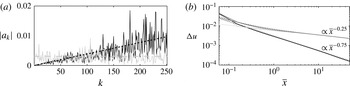
). The wake decay of the imperfect wire position zither differs significantly to a zither with only imperfect source strength, predominately due to the respective
 $\overline{x}^{-0.75}$
and
 $\overline{x}^{-0.25}$
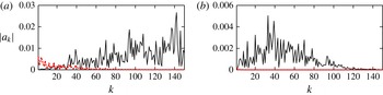
dependencies. For the same standard deviation of imperfection, the zither with only source strength variation will be weaker close to the zither, but stronger far downstream. The wake decay is explained by the Fourier coefficient distributions shown in figure 2. The distribution for a zither with only variation in wire position is approximated by,
 $$\begin{eqnarray}a_{kP}=\frac{2{\rm\pi}k{\it\sigma}_{{\it\delta}}\overline{q}}{M\sqrt{N}}.\end{eqnarray}$$
The distribution for variation only in source strength is approximated as,
 $$\begin{eqnarray}a_{kD}=\frac{{\it\sigma}_{{\it\epsilon}}\overline{q}}{M\sqrt{N}}.\end{eqnarray}$$
Variation in wire source strength can create significantly stronger small wavenumbers (large wavelengths), that decay slower and create a stronger far wake. This leads to a hypothesis that significant spanwise variation in the test-section boundary layer is linked to screens that have significant spatial variation of source strength. This spatial variation may be induced by poor quality screens that have larger variations in wire position which, particularly for lower open-area ratios, may lead to nearby wires influencing each other’s source strength (drag) and creating a stronger far wake.
(a) Fourier coefficients at the zither due to: grey solid line, random normal distribution of wire drag; grey dashed, mean distribution of drag, (2.21); black solid, random normal distribution of wire position; black dashed, mean distribution of position, (2.20). (b) Example wake decay: light grey solid, random normal distribution of wire drag calculated with (2.18) and (2.4); light grey dashed, variation of drag, (2.19); black solid, random normal distribution of wire position calculated with (2.16) and (2.4); black dashed, variation of position, (2.17); dark grey solid, random normal distribution of wire drag and position calculated with (2.8) and (2.4); dark grey dashed, variation of drag and position, the combined wake strength equation, (2.15).

2.6. Zither CFD domain and methods
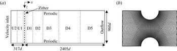
Navier–Stokes simulations (CFD) will be used to study ten zithers with differing combinations of open-area ratio and random wire position error. The steady, pressure-based solver (second-order upwind differencing for pressure, third-order MUSCL differencing for momentum) of the ANSYS Fluent CFD package is used. Solution convergence is judged by the constancy of the far wake with increasing iteration and convergence of global residual monitors. An overview of the zither domain and mesh is shown in figure 3(a). The velocity inlet-boundary-condition is 317 diameters (d) (80.47 mm) upstream of the zither while the outflow boundary condition is located at
 $2405d$
(610.8 mm). Periodic boundary conditions are used in the spanwise direction.
To reduce the total mesh control volumes (CV), eight regions with varying resolution are used as the wake spanwise scale increases. Each region is composed of structured quadrilateral CV aligned with the uniform flow direction. Hanging nodes are used to halve the number CV in the spanwise direction at each region boundary. Figure 3(b) shows the mesh between wires. There are 216 CV on the surface of a wire. Total mesh size varies between 23.4 and 44.2 million CV, depending on the open-area ratio. Refining the entire
 ${\it\beta}=60\,\%$
with
 ${\it\sigma}_{{\it\delta}}=0.05$
mesh by a factor 2 in each direction altered wire forces by less than 0.5 % and has a negligible effect on the far wake (see figure 4
c).
The spanwise domain is the same for all zithers (
 $L=243.84$
mm), with up to 576 wires depending on the open-area ratio (see table 1). Numerical tests comparing (2.2) with (2.15) show this is enough wires for the averaging in (2.15) to be representative beyond
 $\overline{x}=30$
(see Pook Reference Pook2013). The spanwise domain is also more than six times wider than the wavelength for optimal, non-modal streak growth (Andersson et al.
Reference Andersson, Berggren and Henningson1999) at the downstream end of the model test section used in § 4.
(a) Overview of the zither mesh domain. Marked regions start at streamwise positions: U2 at
 $-317d$
, U1 at
 $-76d$
, Zither at
 $-7d$
to 7
 $d$
, D1 at 7
 $d$
, D2 at 67
 $d$
, D3 at 205
 $d$
, D4 at 405
 $d$
, D5 at 805
 $d$
. (b) Close-up of the CFD mesh between two zither wires. Every second line shown.

2.7. Zither geometry
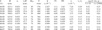
Table 1 lists the geometry parameters for all the zithers which are composed of circular wires arranged in a line perpendicular to the free stream. All wires have a diameter of 254
 ${\rm\mu}$
m, the same size used by Pook & Watmuff (Reference Pook and Watmuff2014). Four open-area ratios (
 ${\it\beta}$
) are used,
 ${\it\beta}=40\,\%$
where coalescence of jets is expected, 50 %, 60 % and 66.67 % where coalescence of jets is not expected. The open-area ratio, diameter and the mesh spacing of the perfect zither (uniformly spaced wires) are related by,
 $$\begin{eqnarray}{\it\beta}=1-\frac{d}{M}.\end{eqnarray}$$
Each wire (
 $n$
) is randomly perturbed from its position in the perfect zither by some distance. A normal distribution is used for the random variation of
 ${\it\delta}_{n}$
, with (near) zero mean and a given standard deviation (
 ${\it\sigma}_{{\it\delta}}$
) listed in table 1 (see Pook Reference Pook2013 for quantile-quantile plots). The
 ${\it\beta}=60\,\%$
zithers share the same distribution of
 ${\it\delta}_{n}$
, i.e. the differing standard deviation is achieved by multiplying by a constant. The same applies for the
 ${\it\beta}=66.67\,\%$
zithers. The
 ${\it\beta}=50\,\%$
zithers all have differing distributions. A constant
 ${\it\sigma}_{{\it\delta}}$
implies a decreasing physical error in wire position with decreasing open-area ratio. The largest standard deviation in physical units for the zithers studied is 57.1
 ${\rm\mu}$
m, or 22 % of the wire diameter. The smallest is 10
 ${\rm\mu}$
m, or 4 % of the wire diameter. The uniform free stream is
 $U=1.7$
m s
 $^{-1}$
giving a Reynolds number based on wire diameter
 $Re_{d}=29.6$
for all zithers, except the
 ${\it\beta}=66.67$
% with
 ${\it\sigma}_{{\it\delta}}=0.05$
zither that uses
 $U=1.9$
m s
 $^{-1}$
. The zithers are sub-critical (do not shed eddies).
Zither wake strength from CFD simulations compared to prediction: (a)
 ${\it\beta}=40\,\%$
; (b)
 ${\it\beta}=50\,\%$
; (c)
 ${\it\beta}=60\,\%$
; (d)
 ${\it\beta}=66.67\,\%$
. Lines: - - - - prediction due to only position variation (2.17);
 $\cdots \cdots$
prediction of combined wake strength (2.15);

 ${\it\sigma}_{{\it\delta}}=0.025$
;

 ${\it\sigma}_{{\it\delta}}=0.05$
;

 ${\it\sigma}_{{\it\delta}}=0.075$
;

 ${\it\sigma}_{{\it\delta}}=0.1$
. For (b),

 ${\it\sigma}_{{\it\delta}}=0.05$
.

Table 1 shows that the mean wire source strength is (near) invariant to the standard deviation of wire position variation. The wire source strength is obtained from the CFD wire force data and the mean calculated by,
 $$\begin{eqnarray}\overline{q}=\frac{1}{{\it\rho}UN}\mathop{\sum }_{n=1}^{N}D_{n}.\end{eqnarray}$$
The drag coefficient (
 $C_{d}$
) is defined as
 $D=0.5{\it\rho}U^{2}dC_{d}$
. The pressure drop coefficient (
 $PD={\rm\Delta}p/(0.5{\it\rho}U^{2})$
) is also listed.
Zither geometry, source strength data and wake strength at
 $\overline{x}=10$
and
 $x=2300d$
.

2.8. Wake strength
Figure 4 compares the CFD wake strength with the predicted wake strength due only to variation in wire position (2.17), and the combined wake strength equation (2.15). Beyond
 $\overline{x}\gtrsim 0.1$
, the CFD wakes decay as
 $\overline{x}^{-0.75}$
. However, at
 $\overline{x}=1$
, the CFD wake strengths are 20–40 % greater than predicted by (2.17) (see Pook Reference Pook2013), with the error increasing with the standard deviation of wire position variation (
 ${\it\sigma}_{{\it\delta}}$
) and decreasing open-area ratio. By
 $\overline{x}=10$
, the CFD wake strengths are 20–70 % stronger, indicating a decay-rate slower than
 $\overline{x}^{-0.75}$
but not nearly as dramatic as predicted by (2.15).
(a) The effect of a downstream initial condition for the
 ${\it\beta}=40\,\%$
,
 ${\it\sigma}_{{\it\delta}}=0.025$
zither. —— CFD; - - - - calculated with (2.1) and (2.8);

 $\overline{x}=0.13$
;

 $\overline{x}=2.5$
. (b)
 ${\it\beta}=50\,\%$
zithers CFD wake strength compared to calculation with (2.1) and (2.8). Lines and markers as for figure 2.

FFT of streamwise velocity and pressure for the
 ${\it\beta}=40\,\%$
,
 ${\it\sigma}_{{\it\delta}}=0.025$
zither: (a)
 $\overline{x}=0.13$
; (b)
 $\overline{x}=2.5$
. Lines: —— streamwise velocity; - - - - pressure.

Table 1 shows
 ${\it\sigma}_{{\it\epsilon}}/{\it\sigma}_{{\it\delta}}$
is a near constant 0.13 for the
 ${\it\beta}=60\,\%$
and
 ${\it\beta}=66.67\,\%$
zithers when
 ${\it\sigma}_{{\it\delta}}\leqslant 0.05$
. The wake strength at a given streamwise distance for the
 ${\it\beta}=60\,\%$
and 66.67 % zithers scales near linearly with
 ${\it\sigma}_{{\it\delta}}$
. However, the
 ${\it\beta}=50\,\%$
zithers show linear scaling only for
 ${\it\sigma}_{{\it\delta}}=0.025$
and 0.05. The
 ${\it\sigma}_{{\it\delta}}=0.075$
zither wake strength is significantly greater than a linear scaling, indicating the wake strength due to only variation in wire position (2.17) does not predict the correct wake decay for zithers with large
 ${\it\sigma}_{{\it\delta}}$
which induces variations of drag across the zither. With decreasing open-area ratio, the ratio
 ${\it\sigma}_{{\it\epsilon}}/{\it\sigma}_{{\it\delta}}$
is seen to increase but only substantially for the
 ${\it\beta}=40\,\%$
zither. However, its wake decay proportional to
 $\overline{x}^{-0.75}$
indicates a flawed assumption in the derivation of the combined wake strength equation (2.15).
2.9. Validity of the linear diffusion equation
The
 ${\it\beta}=40\,\%$
zither CFD wake is sampled and used as a downstream initial condition to (2.1) as validation. Figure 5 shows using an initial condition sampled at
 $\overline{x}=2.5$
where
 ${\rm\Delta}u=1\,\%$
, predicts a downstream wake in agreement with CFD. Using a fast Fourier transform (FFT) on the sampled wakes, figure 6, shows an initial condition too close to the zither fails as low-wavenumber variations of pressure have not been recovered into velocity. Fourier coefficients calculated at the zither with both wire drag and drag position are used to predict the wake in figure 5. The predicted wake undershoots the CFD results between
 $\overline{x}=0.1$
and
 $\overline{x}=6$
, before showing reasonable agreement further downstream. As wire drag includes the effect of pressure, the linear diffusion equation can be used with known wire drag to predict the far wake.
The relative error between CFD wake strength and (2.1) using known wire drag is less than 10 % for
 $\overline{x}>1$
, for all zithers. Equation (2.17) under-predicts wake strength primarily because it neglects the variation in wire drag.
Fourier coefficients at the zither due to variation in drag only, calculated with (2.18): (a)
 ${\it\beta}=40\,\%$
; (b)
 ${\it\beta}=50\,\%$
; (c)
 ${\it\beta}=60\,\%$
; (d)
 ${\it\beta}=66.67\,\%$
.Increasing coefficients is increasing
 ${\it\sigma}_{{\it\delta}}$
. Lines: black,
 ${\it\sigma}_{{\it\delta}}=0.025$
; red,
 ${\it\sigma}_{{\it\delta}}=0.05$
; blue,
 ${\it\sigma}_{{\it\delta}}=0.075$
; green,
 ${\it\sigma}_{{\it\delta}}=0.1$
.

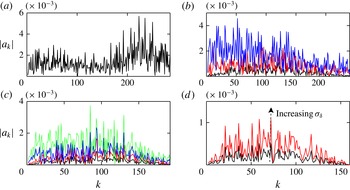
2.10. Distribution of source strength (drag)
Figure 7 shows the Fourier spectra due to only variation in wire drag, calculated with (2.18). The magnitude of the
 ${\it\beta}=60\,\%$
and 66.67 % zither Fourier coefficients increase from
 $k=0$
, peak at approximately
 $k=100$
, before diminishing. Approximating with the mean Fourier coefficient, as
 $a_{kD}$
does, will significantly over estimate the effect of wire drag variation for large wavelengths. The combined wake equation will over predict the wake strength at large
 $\overline{x}$
. For
 ${\it\beta}=50\,\%$
, the Fourier coefficients for small
 $k$
increase with
 ${\it\sigma}_{{\it\delta}}$
. Only for the
 ${\it\sigma}_{{\it\delta}}=0.75$
zither are the Fourier coefficients spread relatively evenly across the spectrum at low wavenumbers, meaning
 ${\it\sigma}_{{\it\epsilon}}$
should be an accurate representation. The wake decay should reduce from
 $\overline{x}^{-0.75}$
at large streamwise distances. Indeed, figure 4 does show the wake decay reducing for this zither.
The Fourier spectrum of the
 ${\it\beta}=40\,\%$
zither is different to the other zithers, with the largest coefficients occurring at wavenumbers
 $k>200$
, raising
 ${\it\sigma}_{{\it\epsilon}}$
but not affecting the far wake. A wavenumber of
 $k=288$
corresponds to a wavelength of
 $2M$
, i.e. a wavelength that could be expected to be associated with the coalescence of adjacent jets.
The over prediction of wake strength by the combined wake strength equation (2.15) is attributed to the assumed Fourier coefficient distribution due to variation in wire source strength (drag),
 $a_{kD}$
. Approximating the Fourier coefficients due to wire force variation as constant (independent of
 $k$
) is not valid and over predicts the wake strength for large
 $\overline{x}$
. Equations to predict wake strength more accurately require an understanding of how the drag of a wire varies with an error in its position, particularly at low wavenumbers.
2.11. Wake wavelength
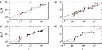
The dominant wavelength at each streamwise position is extracted from the CFD wakes using an FFT of the streamwise velocity. Figure 8 shows the dominant wavelength increases with
 $\overline{x}^{0.5}$
and is independent of the zither geometry, as predicted by (2.14). Wake profiles can also be calculated from knowledge of the individual wire source strength and position data (see Pook Reference Pook2013).


2.12. Coalescence of jets
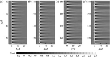
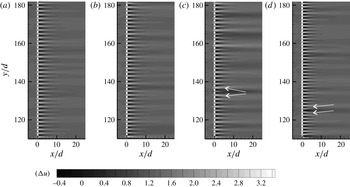
Figures 9 and 10 show contours of streamwise velocity for a limited extent (
 ${<}$
10 %) of the
 ${\it\beta}=40\,\%$
, 50 % and 60 % zithers. The
 ${\it\beta}=60\,\%$
zithers share the same wire perturbation pattern. Apart from the longer jets and wakes, the flow pattern does not significantly change over the
 ${\it\sigma}_{{\it\delta}}$
range investigated. There is minimal deflection of the jets that would be taken to indicate the coalescence of jets in experimental flow visualisation (see Bradshaw Reference Bradshaw1965; Le Gal et al.
Reference Le Gal, Peschard, Chauve and Takeda1996), and table 1 shows
 ${\it\sigma}_{{\it\epsilon}}/{\it\sigma}_{{\it\delta}}$
is near constant. For the
 ${\it\beta}=50\,\%$
with
 ${\it\sigma}_{{\it\delta}}=0.075$
zither shown in figure 10(c), the jets emanating near the cylinder at
 $z/d\approx 135$
are visibly deflected away from each other, creating an extended region of low-speed flow. More instances of visible jet deflection can be observed for this zither, and particularly the
 ${\it\beta}=40\,\%$
zither, but not the other zithers. The ratio
 ${\it\sigma}_{{\it\epsilon}}/{\it\sigma}_{{\it\delta}}$
increases for zithers with instances of jet deflection.
The observed instances of jet deflection in figure 10 are similar to the experimental flow visualisations of Le Gal et al. (Reference Le Gal, Peschard, Chauve and Takeda1996). However, Le Gal et al. (Reference Le Gal, Peschard, Chauve and Takeda1996) observed significant jet deflection for the majority of jets. As previously mentioned, the Fourier coefficients of the
 ${\it\beta}=40\,\%$
zither wire drag increase rapidly for
 $k>200$
. This indicates a flow pattern that possibly correlates to the coalescence of jets. However, such small wavelengths have no effect on the far wake strength. For all other zithers, there is no trend towards increased drag variation at wavelengths approaching
 $2M$
relative to large wavelength, although the Fourier coefficients for the
 ${\it\beta}=50\,\%$
with
 ${\it\sigma}_{{\it\delta}}=0.075$
are appreciable at short wavelengths. The authors’ opinion is that the coalescence of jet phenomena (large jet deflection visible in contours) appears for a limited number of jets in the
 ${\it\beta}=40\,\%$
and to a lesser extent the
 ${\it\beta}=50\,\%$
with
 ${\it\sigma}_{{\it\delta}}=0.075$
zithers. This differs from the flow visualisations of Bradshaw (Reference Bradshaw1965) and Le Gal et al. (Reference Le Gal, Peschard, Chauve and Takeda1996) where the majority of jets show large deflection.
Contours of streamwise velocity scaled by free-stream velocity
 $U$
(see insert for scale) for a limited extent (
 ${<}$
10 %) of the zithers,
 ${\it\beta}=60\,\%$
with: (a)
 ${\it\sigma}_{{\it\delta}}=0.025$
,
 ${\it\sigma}_{{\it\epsilon}}/{\it\sigma}_{{\it\delta}}=0.13$
; (b)
 ${\it\sigma}_{{\it\delta}}=0.05$
,
 ${\it\sigma}_{{\it\epsilon}}/{\it\sigma}_{{\it\delta}}=0.13$
; (c)
 ${\it\sigma}_{{\it\delta}}=0.075$
,
 ${\it\sigma}_{{\it\epsilon}}/{\it\sigma}_{{\it\delta}}=0.13$
; (d)
 ${\it\sigma}_{{\it\delta}}=0.1$
,
 ${\it\sigma}_{{\it\epsilon}}/{\it\sigma}_{{\it\delta}}=0.17$
.

Contours of streamwise velocity scaled by free-stream velocity
 $U$
(see insert for scale) for limited extent (
 ${<}$
10 %) of the zithers: (a)
 ${\it\beta}=50\,\%$
with
 ${\it\sigma}_{{\it\delta}}=0.025$
,
 ${\it\sigma}_{{\it\epsilon}}/{\it\sigma}_{{\it\delta}}=0.13$
; (b)
 ${\it\beta}=50\,\%$
with
 ${\it\sigma}_{{\it\delta}}=0.05$
,
 ${\it\sigma}_{{\it\epsilon}}/{\it\sigma}_{{\it\delta}}=0.14$
; (c)
 ${\it\beta}=50\,\%$
with
 ${\it\sigma}_{{\it\delta}}=0.075$
,
 ${\it\sigma}_{{\it\epsilon}}/{\it\sigma}_{{\it\delta}}=0.18$
; (d)
 ${\it\beta}=40\,\%$
with
 ${\it\sigma}_{{\it\delta}}=0.025$
,
 ${\it\sigma}_{{\it\epsilon}}/{\it\sigma}_{{\it\delta}}=0.29$
. Arrows indicate examples of significant jet deflection.

2.13. The effect of non-uniform inflow
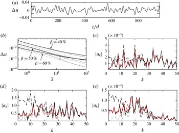
Limited CFD simulations are performed with a random inlet-velocity wake
 $(U_{r})$
, constructed by the addition of sinusoids, from
 $k=1$
to 50, with random phase,
 $$\begin{eqnarray}U_{r}=U+\mathop{\sum }_{k=1}^{50}0.002U\sin \left(\frac{2{\rm\pi}k}{960}\frac{z}{d}+\text{random phase}\right).\end{eqnarray}$$
The non-uniform inflow strength is
 ${\rm\Delta}u=1\,\%$
and the profile is shown in figure 11(a). The non-uniform inflow is applied to the
 ${\it\beta}=40\,\%$
, 50 % and 60 % zithers with
 ${\it\sigma}_{{\it\delta}}=0.025$
. The streamwise domains of the
 ${\it\beta}=40\,\%$
and 50 % zithers are extended to capture any change of wake decay.
(a) Non-uniform velocity inlet profile. (b) Wake strength,
 ${\it\beta}=40\,\%$
, 50 %, 60 % with
 ${\it\sigma}_{{\it\delta}}=0.025$
zithers. Dark solid line (stronger far wake) is non-uniform inflow. Light solid line is uniform inflow. Square makers indicated strength downstream calculated with (2.2). Dashed lines are (2.17). (c) Fourier coefficients at
 $\overline{x}=10$
for
 ${\it\beta}=40\,\%$
. (d) Fourier coefficients at
 $\overline{x}=10$
for
 ${\it\beta}=50\,\%$
. (e) Fourier coefficients at
 $\overline{x}=10$
for
 ${\it\beta}=60\,\%$
. Lines: black solid, extracted from CFD with non-uniform inflow; grey dash-dot, extracted from CFD with uniform inflow; black long-dash, calculated with (2.8) at zither and transferred to
 $\overline{x}=10$
with (2.5); red short-dash, calculated with (2.25) at zither and transferred to
 $\overline{x}=10$
with (2.5).

Velocity contours near the zither (not shown) are not discernibly different to the uniform inflow simulations. For small
 $\overline{x}$
, figure 11(b) shows the non-uniform inflow wake decay changes from
 $\bar{x}^{-0.75}$
towards
 $\bar{x}^{-0.25}$
. This is readily apparent for the
 ${\it\beta}=60\,\%$
zither. For
 $\overline{x}>13$
, the
 ${\it\beta}=60\,\%$
zither wake is stronger than the
 ${\it\beta}=50\,\%$
zither.
At
 $\overline{x}=10$
, the
 ${\it\beta}=60\,\%$
zither non-uniform inlet wake strength is 50 % greater relative to a uniform inflow. The
 ${\it\beta}=50\,\%$
zither wake is 16 % greater and the
 ${\it\beta}=40\,\%$
zither is only 9 % greater. Standard deviations of wire source strength (
 ${\it\sigma}_{{\it\epsilon}}$
) for the
 ${\it\beta}=40\,\%$
, 50 % and
 ${\it\beta}=60\,\%$
zithers are 0.0093, 0.0045 and 0.0058, respectively. As
 ${\it\sigma}_{{\it\delta}}$
is the same, the combined wake-strength equation (2.15) would predict the
 ${\it\beta}=40\,\%$
zither wake to show a greater deviation from
 $\overline{x}^{-0.75}$
, opposite to what is observed in figure 11(b).
Wake Fourier coefficients at
 $\overline{x}=10$
are extracted from the CFD simulations and shown in figure 11(c–e) for the uniform and non-uniform inlet simulations. Also shown are the Fourier coefficients calculated from the individual wire drag and position data, and transferred to
 $\overline{x}=10$
by (2.5). The extracted Fourier coefficients at low wavenumbers are significantly smaller than calculated with wire position and drag data. This increases the calculated value of
 ${\it\sigma}_{{\it\epsilon}}$
relative to that observed. Decreasing open-area ratio reduces the difference between uniform and non-uniform inflow Fourier coefficients. The drag variation induced at the zither by the non-uniform inflow, creates an additional wake component tending to cancel the non-uniform inflow. The removal of a non-uniform inflow with increasing screen pressure drops is predicted by the Taylor & Batchelor (Reference Taylor and Batchelor1949) analysis. Hence, the far wake strength of the lower-open area ratio zithers with a non-uniform inflows differs less compared to a uniform inflow.
Prediction of the far wake with known wire position and drag data can be improved by linearly adding the non-uniform inlet velocity. The Fourier coefficients at the zither are then found as,
 $$\begin{eqnarray}a_{k}=\frac{\overline{q}}{L}\mathop{\sum }_{n=1}^{N}(-2{\rm\pi}\text{i}K{\it\delta}_{n}+{\it\epsilon}_{n}-2{\rm\pi}\text{i}K{\it\epsilon}_{n}{\it\delta}_{n})\exp (-2{\rm\pi}\text{i}Kn)-a_{kw},\end{eqnarray}$$
where
 $a_{kw}$
is the
 $k$
th Fourier coefficient of the non-uniform inflow at the zither, assuming no influence of the zither. It is subtracted due to the convention of a wake being positive. Figure 11(c–e) reveals the addition of the non-uniform inflow term produces good agreement between the calculated and CFD Fourier coefficients.
3. Zither wakes through the contraction
The zither wakes of normal vorticity pass through a contraction which removes the majority of the
 ${\rm\Delta}u$
wake component and produces streamwise vorticity. The uniform-inflow zither wakes are sampled
 $197d$
downstream of the zither and imposed
 $957d$
upstream of the contraction start. Symmetry requires only the lower-half of the 5:1, two-dimensional contraction to be modelled. A structured mesh with quadrilateral CV is used, with 440, 200 and 500 CV in the streamwise, wall-normal and spanwise directions. This is the same geometry and similar mesh resolution used by Pook & Watmuff (Reference Pook and Watmuff2014) to accurately reproduce the effect of a single wire wake passing through a contraction by comparison with the experiment of Watmuff (Reference Watmuff2006).
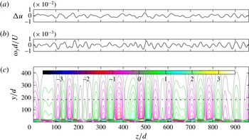
Figure 12 provides an example of a two-dimensional zither wake entering the contraction and contours of the streamwise vorticity (
 ${\it\omega}_{x}$
) on a plane
 $394d$
downstream of the exit, scaled by the standard deviation of the normal vorticity entering the contraction (
 ${\it\sigma}_{{\it\omega}y\,\mathit{in}}$
). The contraction floor is located at
 $y/d=0$
on the downstream plane and the leading edge used in § 4 is located at
 $y=186d$
. Stronger regions of streamwise vorticity near the contraction floor are due to the combination of Görtler instability near the no-slip contraction wall combined with the tilting and stretching mechanism discussed by Pook & Watmuff (Reference Pook and Watmuff2014). The visible wake spanwise wavelength changes little through the contraction. The magnitude of the streamwise vorticity reduces to zero at the contraction centreline.
Wake of the
 ${\it\beta}=50\,\%$
with
 ${\it\sigma}_{{\it\delta}}=0.025$
zither entering the contraction and streamwise vorticity out. (a) Wake spanwise profile of
 ${\rm\Delta}u$
entering contraction. (b) Wake spanwise profile of normal vorticity (
 ${\it\omega}_{y}$
) entering contraction. (c) Contours of streamwise vorticity (
 ${\it\omega}_{x}/{\it\sigma}_{{\it\omega}y\,\mathit{in}}$
), 394
 $d$
downstream of the contraction exit. Dashed line is leading edge of § 4.

Streamwise vorticity
 $394d$
downstream of the contraction exit,
 $186d$
above the contraction floor: (a)
 ${\it\beta}=40\,\%$
; (b)
 ${\it\beta}=50\,\%$
; (c)
 ${\it\beta}=60\,\%$
; (d)
 ${\it\beta}=66.67\,\%$
. Lines: black,
 ${\it\sigma}_{{\it\delta}}=0.025$
; red,
 ${\it\sigma}_{{\it\delta}}=0.05$
; blue,
 ${\it\sigma}_{{\it\delta}}=0.075$
; green,
 ${\it\sigma}_{{\it\delta}}=0.1$
.

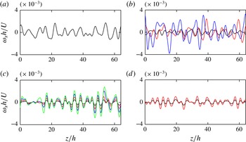
A spanwise profile of streamwise vorticity at the contraction exit is shown in figure 13. The zither with the strongest wake,
 ${\it\beta}=50\,\%$
with
 ${\it\sigma}_{{\it\delta}}=0.075$
, produces the strongest streamwise vorticity. The maximum streamwise velocity perturbation on a spanwise profile 11 leading edge half-thicknesses (
 $h$
) upstream of the leading edge, is less than 0.015 % of
 $U$
(not shown). The streamwise vorticity is predominantly due to spanwise variation of the wake normal velocity perturbation (maximum of
 ${\sim}$
0.5 % of
 $U$
), giving a flow angle of
 $0.26^{\circ }$
. However, the standard deviation of the flow angle is only
 $0.1^{\circ }$
and is a better indicator of what would be measured by a survey of flow quality.
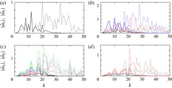
An FFT on the spanwise profile of streamwise vorticity exiting, and normal vorticity entering, is shown in figure 14. The largest streamwise vorticity coefficient occurs at
 $k=10$
–12 for all zithers, except the
 ${\it\beta}=66.67\,\%$
zithers which have three peaks from
 $k=11$
to 21. At this height above the floor, wavenumbers below
 $k\approx 10$
exhibit a larger streamwise vorticity Fourier coefficient than the normal vorticity, while for
 $k>30$
the coefficients are negligible at the contraction exit.
Streamwise vorticity FFT (
 $\hat{{\it\omega}}_{x}$
, solid lines) magnitude,
 $394d$
downstream of the contraction exit,
 $186d$
above the contraction floor. Normal vorticity (
 $\hat{{\it\omega}}_{y}$
, dotted lines) magnitude at contraction start. (a)
 ${\it\beta}=40\,\%$
; (b)
 ${\it\beta}=50\,\%$
; (c)
 ${\it\beta}=60\,\%$
; (d)
 ${\it\beta}=66.67\,\%$
. Lines: black,
 ${\it\sigma}_{{\it\delta}}=0.025$
; red,
 ${\it\sigma}_{{\it\delta}}=0.05$
; blue,
 ${\it\sigma}_{{\it\delta}}=0.075$
; green,
 ${\it\sigma}_{{\it\delta}}=0.1$
.

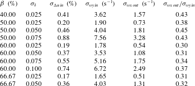
Table 2 lists the standard deviation of the normal vorticity entering the contraction (
 ${\it\sigma}_{{\it\omega}y\,\mathit{in}}$
), and the standard deviation of the streamwise vorticity on the spanwise profile after the contraction, at the height of the leading edge to be used in § 4, (
 ${\it\sigma}_{{\it\omega}x\,\mathit{out}}$
). The ratio varies between 0.30 and 0.45, increasing with a decrease in screen open-area ratio and increase in
 ${\it\sigma}_{{\it\delta}}$
. This indicates differing wake decay rates in the contraction.
The zither wake decay through the contraction (
 ${\rm\Delta}u_{c}$
) is examined with the ratio,
 $$\begin{eqnarray}{\rm\Delta}u_{c}=\frac{{\rm\Delta}u_{local}}{{\rm\Delta}u_{0}},\end{eqnarray}$$
where
 ${\rm\Delta}u_{local}$
is the wake strength on the contraction centreline normalised by the local velocity on the contraction centreline, and
 ${\rm\Delta}u_{0}$
is the zither wake strength at the contraction entry. Figure 15 plots (3.1). At the contraction exit, the value of
 ${\rm\Delta}u_{c}$
for the strongest zither wake is twice that of the weakest. Zithers with relatively larger low-wavenumbers of drag variation (see figure 7) have a stronger wake exiting the contraction, indicating the importance of large-wavelength drag variation across the zither. The trend in figure 15 holds across a contraction cross section.
Scaled wake strength on the contraction centreline,
 ${\rm\Delta}u_{cont}$
defined by (3.1). The contraction curvature begins at
 $x/L_{c}=0$
and ends at
 $x/L_{c}=1$
,
 $L_{c}=1.524$
m. Lines:

 ${\it\beta}=40\,\%$
 ${\it\sigma}_{{\it\delta}}=0.025$
;

 ${\it\beta}=50\,\%$
 ${\it\sigma}_{{\it\delta}}=0.025$
;

 ${\it\beta}=50\,\%$
 ${\it\sigma}_{{\it\delta}}=0.05$
;

 ${\it\beta}=50\,\%$
 ${\it\sigma}_{{\it\delta}}=0.075$
;

 ${\it\beta}=60\,\%$
 ${\it\sigma}_{{\it\delta}}=0.025$
;

 ${\it\beta}=60\,\%$
 ${\it\sigma}_{{\it\delta}}=0.05$
;

 ${\it\beta}=60\,\%$
 ${\it\sigma}_{{\it\delta}}=0.075$
;

 ${\it\beta}=60\,\%$
 ${\it\sigma}_{{\it\delta}}=0.1$
;

 ${\it\beta}=66\,\%$
 ${\it\sigma}_{{\it\delta}}=0.025$
.

Ratio of
 ${\it\sigma}_{{\it\omega}x\,\mathit{out}}$
to
 ${\it\sigma}_{{\it\omega}y\,\mathit{in}}$
on a profile
 $394d$
downstream of contraction exit and
 $186d$
above contraction floor.

4. Test section flat-plate boundary layer
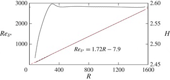
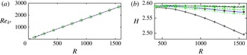
The streamwise vorticity exiting the contraction creates streaks in the test-section plate boundary layer. Receptivity to low-frequency streamwise vorticity has been shown by Schrader et al. (Reference Schrader, Brandt, Mavriplis and Henningson2010) to be a dominant mechanism. The same leading edge geometry as Pook & Watmuff (Reference Pook and Watmuff2014) with a slot mass-flow of 0.21 is used (see Pook & Watmuff (Reference Pook and Watmuff2014) for details). Near Blasius flow is achieved by
 $R=400$
, where
 $R=\sqrt{Ux/{\it\nu}}$
, as indicated by the shape factor in figure 16. The virtual origin is small and of little consequence to the results presented. Shifting the attachment point has a minimal effect on the receptivity to streamwise vorticity (Pook & Watmuff Reference Pook and Watmuff2014). The free-stream velocity over the flat-plate region is
 $U=8.6$
m s
 $^{-1}$
.
The mesh in the test-section boundary layer has minimal skewness with
 ${\sim}$
40 CV in the wall-normal direction and
 ${\sim}$
500 CV in the spanwise direction. The total mesh size is
 ${\sim}$
45 million CV. This is a similar level of refinement as Mesh
 $_{2}$
in Pook & Watmuff (Reference Pook and Watmuff2014) that was shown to accurately calculate the streak strength.
Two-dimensional base flow. Reynolds number based on displacement thickness (
 $Re_{{\it\delta}^{\ast }}$
) versus
 $R$
and shape factor (
 $H$
) versus
 $R$
. Blasius displacement thickness growth shown with - - - -. Equation is fit to CFD data. The leading edge ends at
 $R=345$
.

4.1. Measures of streak strength
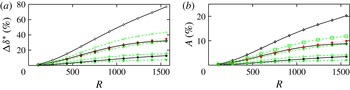
Various measures of streak strength have been favoured in the literature with no direct relations provided between them. Figure 17(a) documents streak strength (
 ${\rm\Delta}{\it\delta}^{\ast }$
) as measured by the maximum and minimum displacement thickness on a given cross-sectional plane,
 $$\begin{eqnarray}{\rm\Delta}{\it\delta}^{\ast }=\frac{\displaystyle \max _{y,z}({\it\delta}^{\ast })-\displaystyle \min _{y,z}({\it\delta}^{\ast })}{{\it\delta}_{b}^{\ast }},\end{eqnarray}$$
where the subscript
 $b$
indicates the two-dimensional flow with no streaks. Figure 17(b) shows the corresponding streak amplitude (
 $A$
) defined by,
 $$\begin{eqnarray}A=\frac{\displaystyle \max _{y,z}(U-U_{b})-\displaystyle \min _{y,z}(U-U_{b})}{2U}.\end{eqnarray}$$
Both measures are linear with
 $x^{0.5}$
, downstream of an initial receptivity region, until
 $R\approx 1000$
.
(a) Streak strength
 ${\rm\Delta}{\it\delta}^{\ast }$
versus
 $R$
. (b) Streak amplitude (
 $A$
) versus
 $R$
. Lines and markers as for figure 15.

The ratio of
 ${\rm\Delta}{\it\delta}^{\ast }$
to
 $A$
beyond
 $R>400$
is approximately 3.6 for all zithers except the
 ${\it\beta}=40\,\%$
with
 ${\it\sigma}_{{\it\delta}}=0.075$
and
 ${\it\beta}=50\,\%$
with
 ${\it\sigma}_{{\it\delta}}=0.075$
zithers. For these zithers, the ratio varies between 3.5 and 3.8 with increasing
 $R$
. These zithers have larger amplitude Fourier modes at low wavenumbers. The optimal non-modal growth theory of Andersson et al. (Reference Andersson, Berggren and Henningson1999) and Luchini (Reference Luchini2000) explains that larger spanwise wavelength disturbances will exhibit greater growth and peak further downstream. Indeed, the
 ${\it\beta}=50\,\%$
with
 ${\it\sigma}_{{\it\delta}}=0.075$
zither generates the largest streak growth by a substantial margin with a peak beyond the streamwise domain (
 $R>1600$
). The growth of the weaker zither streaks can be seen to be slowing towards the end of the streamwise domain.
The streak growth qualitatively agrees with the compiled Klebanoff streak data of Westin et al. (Reference Westin, Boiko, Klingmann, Kozlov and Alfredsson1994), which shows linear growth with
 $x^{0.5}$
. Only three data-sets extend beyond
 $R=1500$
, with one set showing a peak and then decrease downstream while the other two show a rapid increase which probably indicates transition. Note the experimental measures of Klebanoff streaks are
 $u_{rms}$
and not directly the streak amplitude measured here.
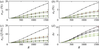
(a) Standard deviation of streak strength
 ${\it\sigma}_{{\rm\Delta}{\it\delta}^{\ast }}$
versus
 $R$
. (b) Standard deviation of streak amplitude
 ${\it\sigma}_{A}$
versus
 $R$
. (c) Standard deviation of normalised skin friction
 ${\it\sigma}_{cf}/\overline{cf}$
versus
 $R$
. (d) Streak strength scaled to zither wake before contraction (
 $As$
) versus
 $R$
. Lines and markers as for figure 15.

Streak strength and amplitude as defined are measures of minimum and maximum deviation from the two-dimensional layer. The standard deviation of these quantities for steady streaks is likely to have a closer relation to the experimental measures of unsteady streaks (e.g.
 $u_{rms}$
) and any possible correlation with TS-wave suppression. The standard deviation of streak strength and amplitude are shown in figure 18. The standard deviation of streak strength (
 ${\it\sigma}_{{\rm\Delta}{\it\delta}^{\ast }}$
) at a given streamwise plane is defined by,
 $$\begin{eqnarray}{\it\sigma}_{{\rm\Delta}{\it\delta}^{\ast }}=\frac{1}{{\it\delta}_{b}^{\ast }}\sqrt{\frac{1}{L}\int _{0}^{L}{\it\delta}^{\ast 2}\,\text{d}z},\end{eqnarray}$$
and the standard deviation of streak amplitude (
 ${\it\sigma}_{A}$
) by,
 $$\begin{eqnarray}{\it\sigma}_{A}=\sqrt{\frac{1}{U^{2}L}\int _{0}^{L}\max _{y,z}(U-U_{b})^{2}\,\text{d}z}.\end{eqnarray}$$
The standard deviation measures are significantly less than the maximal measures but the same relative trends are observed.
Skin friction also provides a measure of streak growth. Figure 18 shows the variation in skin friction defined by,
 $$\begin{eqnarray}{\it\sigma}_{c_{f}}=\frac{2{\it\nu}}{U^{2}}\sqrt{\frac{1}{L}\int _{0}^{L}\left(\frac{\partial U}{\partial y}-\overline{\frac{\partial U}{\partial y}}\right)^{2}\text{d}z},\quad \overline{c_{f}}=\frac{2{\it\nu}}{U^{2}}\overline{\frac{\partial U}{\partial y}},\quad \overline{\frac{\partial U}{\partial y}}=\frac{1}{L}\int _{0}^{L}\frac{\partial U}{\partial y}\,\text{d}z,\end{eqnarray}$$
 $$\begin{eqnarray}{\rm\Delta}c_{f}=\frac{{\it\sigma}_{c_{f}}}{\overline{c_{f}}},\end{eqnarray}$$
where
 ${\rm\Delta}c_{f}$
is the ratio of skin-friction standard deviation to the spanwise mean value, and the wall-normal velocity gradients are measured at the wall. The ratio of
 ${\rm\Delta}c_{f}$
to
 ${\it\sigma}_{A}$
is not constant, varying between 1.65 and 1.9 for the current zither streaks. Skin friction varies between 1.5 % and 18 % at
 $R=1550$
, an order of magnitude variation. Bradshaw (Reference Bradshaw1965) found turbulent skin-friction variation exceeding 10 % when screens with
 ${\it\beta}<57\,\%$
were installed. Only the
 ${\it\beta}=50\,\%$
with
 ${\it\sigma}_{{\it\delta}}=0.075$
zither exceeds 10 %.
Based on the magnitude of skin-friction variation for the
 ${\it\beta}=50\,\%$
with
 ${\it\sigma}_{{\it\delta}}=0.075$
zither, it seems likely that the cause of the spanwise variation in the results of Bradshaw (Reference Bradshaw1965) is also present in the current simulations. Bradshaw (Reference Bradshaw1965) attributed the variation to a spatial ‘instability’ downstream of the screen, leading to the coalescence of jets. The current simulations suggest the cause can be interpreted as being due to the variation of wire drag and wire position across the zither.
4.2. Streak amplitude related to the zither
Ideally, a simple relation can be found to relate streak amplitude to the zither geometry. Relating streak growth to a single measure of velocity variation in the wake will fail, as streak growth is strongly dependent on spanwise wavelength. The relation must be made in terms of vorticity and consider the spectral distribution. However, the current zither wakes do share a similar spanwise wavelength as the zither position is constant and the zither wake wavelength formula was found to be accurate (see figure 8). The contraction and leading edge geometry are also identical. Thus, the streak amplitude can be scaled by the wake strength entering the contraction. If all zither wakes maintain the same wake decay rate, and the streak growth in the test-section layer is linear with amplitude, then a measure of streak amplitude scaled by a measure of the zither wake entering the contraction should collapse to a single curve. Figure 18(d) shows the standard deviation of streak amplitude (
 ${\it\sigma}_{A}$
) scaled by the standard deviation of the zither wake strength entering the contraction (
 ${\it\sigma}_{{\rm\Delta}u/U\,\mathit{in}}$
),
 $$\begin{eqnarray}As=\frac{{\it\sigma}_{A}}{{\it\sigma}_{{\rm\Delta}u/U\,\mathit{in}}}.\end{eqnarray}$$
The
 ${\it\beta}=66.67\,\%$
and
 ${\it\beta}=60\,\%$
zithers with
 ${\it\sigma}_{{\it\delta}}=0.025$
and
 ${\it\sigma}_{{\it\delta}}=0.05$
streak growth collapses with this scaling. However, the
 ${\it\beta}=60\,\%$
zithers with
 ${\it\sigma}_{{\it\delta}}=0.075$
and
 ${\it\sigma}_{{\it\delta}}=0.1$
show an increased scaled streak growth. This indicates a stronger wake, due to a reduced wake decay rate far downstream of the zither. Decreasing
 ${\it\beta}$
for a given
 ${\it\sigma}_{{\it\delta}}$
also increases the scaled streak growth. This is highlighted by the
 ${\it\beta}=40\,\%$
with
 ${\it\sigma}_{{\it\delta}}=0.025$
and
 ${\it\beta}=50\,\%$
with
 ${\it\sigma}_{{\it\delta}}=0.075$
zithers that have nearly identical scaled-streak-growth. Their scaled-streak-amplitude is more than double that for the
 ${\it\beta}=66.67\,\%$
with
 ${\it\sigma}_{{\it\delta}}=0.05$
zither at
 $R=1500$
. Although the dominant Fourier mode in the wake is of a similar wavelength, the spectral distribution is not. Figure 14 shows they have larger amplitude Fourier coefficients below
 $k=10$
, creating larger streaks further downstream. A simple relation between the zither wake strength and the streak amplitude cannot be found.
4.3. Spanwise mean quantities
Figure 19(a) shows the zither streaks have a negligible effect on the spanwise mean displacement thickness, consistent with experimental observations of Klebanoff streaks (Westin et al.
Reference Westin, Boiko, Klingmann, Kozlov and Alfredsson1994). However, figure 19(b) reveals the mean shape factor decreases with streamwise distance relative to the two-dimensional layer. Stronger streaks produce a greater decrease. Westin et al. (Reference Westin, Boiko, Klingmann, Kozlov and Alfredsson1994) reported a decreasing shape factor when FST induced Klebanoff streaks are present, observing a shape factor of 2.41 at
 $R=1260$
. Only the
 ${\it\beta}=50\,\%$
with
 ${\it\sigma}_{{\it\delta}}=0.075$
zither produces a comparable mean shape factor but it occurs further downstream.
(a) Spanwise mean displacement thickness versus
 $R$
. (b) Spanwise mean shape factor (
 $H$
) versus
 $R$
. – ⋅ – ⋅ – Two-dimensional base-flow. Other lines and markers as for figure 15.

4.4. Streak wall-normal velocity profiles
Streaks cause a deviation in the velocity profile relative to the undisturbed two-dimensional base flow. The deviation at a given spanwise position is defined by,
 $$\begin{eqnarray}\frac{{\rm\Delta}U}{U_{e}}=\frac{U-U_{b}}{U_{e}},\end{eqnarray}$$
where
 $U_{e}$
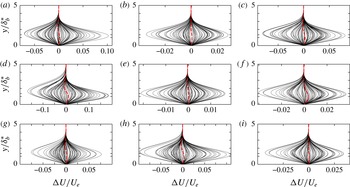
is the edge velocity of the layer. Figure 20 shows zither streak profiles at
 $R=1350$
and a given spanwise position are either all in excess or decrement. The spanwise average of the profiles exhibits an ‘s’-shape, except for the
 ${\it\beta}=60\,\%$
with
 ${\it\sigma}_{{\it\delta}}=0.025$
and
 ${\it\sigma}_{{\it\delta}}=0.05$
zither streaks that have a slight excess across the layer. The ‘s’-shape develops further downstream when the streak amplitude increases. From figure 20, increasing
 ${\it\sigma}_{{\it\delta}}$
(which increases streak amplitude) increases the magnitude of the ‘s’-shape maximum (lower part of ‘s’) and minimum (upper part of ‘s’), approximately 30-fold for the
 ${\it\beta}=50\,\%$
streaks. With increasing
 ${\it\sigma}_{{\it\delta}}$
, the ‘s’-shape maximum moves towards the wall, and the minimum away. This is due to the maximum of local profiles in excess shifting towards the wall, and the minimum of profiles in decrement away. This agrees with the simulations by Jacobs & Durbin (Reference Jacobs and Durbin2001) where backwards jets (unsteady streaks) are lifted to the boundary-layer edge prior to breakdown, and the PIV of Nolan & Walsh (Reference Nolan and Walsh2012) that observed the excess maximum to move towards the wall while the low-speed streak moves away.
The ‘s’-shaped mean profile is similar to the observations of time-averaged, Klebanoff streaks made by Westin et al. (Reference Westin, Boiko, Klingmann, Kozlov and Alfredsson1994) using a grid in the test section to elevate the FST. At
 $R=1350$
the maximum of the ‘s’-shape for the
 ${\it\beta}=50\,\%$
with
 ${\it\sigma}_{{\it\delta}}=0.075$
zither streaks is approximately
 $\max ({\rm\Delta}U/U_{e})\approxeq 0.01$
and the mean shape factor is 2.52, similar to Westin et al. (Reference Westin, Boiko, Klingmann, Kozlov and Alfredsson1994) (
 $\max ({\rm\Delta}U/U_{e})\approxeq 0.011$
when
 $H=2.53$
). However, Kendall (Reference Kendall1985, Reference Kendall1998) measured time-averaged velocity profiles in the presence of Klebanoff streaks at
 $R=980$
, with FST elevated by a grid upstream of the contraction, to be in decrement across the entire layer (
 $\min ({\rm\Delta}U/U_{e})\approxeq -0.02$
). The zither streak results combined with Westin et al. (Reference Westin, Boiko, Klingmann, Kozlov and Alfredsson1994) suggest the difference cannot be attributed solely to a grid location upstream of the contraction.
Wall-normal profiles of
 ${\rm\Delta}U/U_{e}$
, defined by (4.8), at various spanwise positions and
 $R=1350$
. Lines: ——
 ${\rm\Delta}U/U_{e}$
at some spanwise position; - - - - spanwise mean. (a)
 ${\it\beta}=40\,\%$
,
 ${\it\sigma}_{{\it\delta}}=0.025$
; (b)
 ${\it\beta}=50\,\%$
,
 ${\it\sigma}_{{\it\delta}}=0.025$
; (c)
 ${\it\beta}=50\,\%$
,
 ${\it\sigma}_{{\it\delta}}=0.050$
; (d)
 ${\it\beta}=50\,\%$
,
 ${\it\sigma}_{{\it\delta}}=0.075$
; (e)
 ${\it\beta}=60\,\%$
,
 ${\it\sigma}_{{\it\delta}}=0.025$
; (f)
 ${\it\beta}=60\,\%$
,
 ${\it\sigma}_{{\it\delta}}=0.050$
; (g)
 ${\it\beta}=60\,\%$
,
 ${\it\sigma}_{{\it\delta}}=0.075$
; (h)
 ${\it\beta}=60\,\%$
,
 ${\it\sigma}_{{\it\delta}}=0.100$
; (i)
 ${\it\beta}=66.67\,\%$
,
 ${\it\sigma}_{{\it\delta}}=0.025$
.

5. Zither streak linear stability
The analysis suggests the zither streaks share many similarities with Klebanoff streaks, but are steady. If transition is to be predicted accurately in differing wind tunnels, then the methodology must be able to predict transition for the current zither streak base flows. Watmuff (Reference Watmuff1998) observed that initial flow quality improvements related to the settling chamber screens shifted the transition location upstream to a distance 67 % of that observed before the improvements. The computational results of Cossu & Brandt (Reference Cossu and Brandt2004) for the optimal streak would suggest that transition was promoted in the Watmuff (Reference Watmuff1998) wind tunnel as TS-wave growth was previously damped by the presence of streaks. However, Vaughan & Zaki (Reference Vaughan and Zaki2011) found steady, free stream forced streaks with amplitudes
 ${\lesssim}$
15 % can increase TS-wave growth rates. These studies did not use streaks generated from a realistic free-stream disturbance. Parabolized stability equations in three-dimensions (PSE-3D) will be used to assess the linear stability of the zither streak base flows.
PSE-3D is an extension to traditional PSE that allows spanwise variation of the base flow, first presented by Broadhurst & Sherwin (Reference Broadhurst and Sherwin2008). A monochromatic disturbance is described by the product of a shape function on a cross-stream plane, and a spatially growing wave component with a complex streamwise wavenumber (
 ${\it\alpha}$
). The streamwise wavenumber is adjusted marching downstream to keep the total energy of the shape-function constant. A BiGlobal eigenvalue problem provides the initial condition. Details of the numerical implementation can be found in Pook (Reference Pook2013). Unless noted, Chebyshev polynomials are used to difference stability equations in the wall-normal direction with 70 collocation points, and
 $k=25$
Fourier modes are used in the spanwise direction. First-order upwind differencing is used in the streamwise direction.
Conceptually, the PSE-3D can be used with the
 $\text{e}^{N}$
method in place of the Orr–Sommerfeld or two-dimensional PSE equations. This would require a database of streaky base-flow transition results and would inherit all the limitations and assumptions of the
 $\text{e}^{N}$
method, with no guarantee it will be as successful.
5.1. Two-dimensional base-flow linear stability
The linear stability of the two-dimensional base-flow can be measured by the
 $N$
-factor, the ratio of disturbance amplitude growth from Branch 1, which is the streamwise position when the disturbance first becomes unstable. The
 $N$
-factor is defined by,
 $$\begin{eqnarray}N\text{-}\text{factor}=\int _{Branch\,1}^{x}{\it\alpha}_{i}({\it\zeta})\,\text{d}{\it\zeta}.\end{eqnarray}$$
The CFD base flow is of sufficient accuracy to provide results of at least qualitative accuracy (see Pook Reference Pook2013). A resolution check is performed later.
5.2. BiGlobal resolution of the eigenvalue spectrum
The
 ${\it\beta}=50\,\%$
with
 ${\it\sigma}_{{\it\delta}}=0.075$
zither streak base flow at
 $R=940$
(
 $Re_{{\it\delta}^{\ast }}=1615$
) is used to examine spanwise resolution requirements. The streak peak amplitude (
 $A$
) is 12.5 % and the standard deviation of amplitude (
 ${\it\sigma}_{A}$
) is 5.4 %. The BiGlobal eigenvalue spectrum is investigated for a disturbance non-dimensional frequency,
 $F=65$
where,
 $$\begin{eqnarray}F=\frac{{\it\omega}{\it\nu}}{U^{2}}\times 10^{6}.\end{eqnarray}$$
The dimensional circular frequency is 326.8 rad
 $^{-1}$
. For this frequency and position, the two-dimensional base flow is unstable (slightly upstream of Branch 2).
The BiGlobal spectrum, calculated using the modes
 $k=-5$
to 5, is shown in figure 21 (
 ${\it\alpha}_{i}<0$
indicates streamwise growth). The streaky base flow is not symmetric, which prevents using the even/odd assumption to reduce the eigenvalue problem size. The QZ eigenvalue solver (Matlab eig function) is used. The spectrum is similar in appearance to that of two-dimensional Blasius flow. The discrete approximation to the continuous modes can be seen to the left of the spectrum. The spread of the continuous modes is due to the wall-normal differencing not capturing the oscillations of the eigenvectors. Four unstable, discrete eigenvalues can be seen near
 ${\it\alpha}_{r}{\it\delta}_{b}^{\ast }\approxeq 0.3$
.
The eigenvalue spectrum in the region of the unstable eigenvalues is resolved more accurately using an increasing number of spanwise modes and the Arnoldi eigenvalue solver (Matlab eigs function). The increased resolution produces a ‘curved line’ of discrete eigenvalues. Similar to the spectrum for TS modes with varying spanwise wavenumber on a two-dimensional base flow. The most unstable eigenvalue appears by itself. In the limit of two-dimensional flow, without providing direct proof, this mode would correspond to the two-dimensional TS mode. Tracking this mode back towards the leading edge (streak strength decreasing) produces an eigenvector with minimal spanwise variation and an eigenvalue close to that for the two-dimensional layer. It will be called the streaky TS mode following Cossu & Brandt (Reference Cossu and Brandt2004) and labelled A in figure 21. The remaining eigenvalues can be seen to appear in pairs. In the limit of two-dimensional flow they would be the oblique TS modes. They are split because the streaky zither base flow is not spanwise symmetric. They will be called the streaky oblique TS modes and two examples are labelled B and C in figure 21.
The effect of spanwise resolution (Fourier modes
 $k=-N$
to
 $N$
) on the eigenvalues for the
 ${\it\beta}=50\,\%$
,
 ${\it\sigma}_{{\it\delta}}=0.075$
zither at
 $Re_{{\it\delta}^{\ast }}=1615$
(
 $R=940$
). Perturbation frequency is
 $F=65$
,
 ${\it\omega}=326.8~\text{rad}^{-1}$
. A is streak TS mode. B and C are first streaky oblique TS modes. Markers: ●
 $N=5$
and QZ solver;
 $+$
 $N=10$
and Arnoldi Solver; ◻
 $N=15$
and Arnoldi Solver; ○
 $N=20$
and Arnoldi Solver;
 $\times$
 $N=25$
and Arnoldi Solver.

The streaky oblique modes require increased resolution to resolve compared to the streaky TS mode. The convergence of the streaky TS-mode eigenvalue is shown in table 3. It does not change significantly beyond
 $k=20$
. The majority of the streak base-flow energy is in modes
 $k\leqslant 15$
.
Streaky TS-mode convergence with BiGlobal spanwise resolution.

The eigenvectors of labelled eigenvalues A, B and C are shown in figure 22. The
 $u_{rms}$
maxima of the streaky TS is located in high-speed streak regions, while regions of increased
 $u_{rms}$
for the streaky oblique TS are offset from each other in the spanwise direction but remain located in high-speed streak regions. The linear summation of the oblique modes is also shown in figure 22. The eigenvectors have been scaled to have the same total energy prior to addition. The majority of elevated
 $u_{rms}$
for the combined streaky oblique modes is located to the left of
 $z/d=500$
while the streaky TS mode is most elevated in regions to the right of
 $z/d=500$
. The maximum spanwise velocity component of the streaky oblique modes,
 ${\sim}0.6u_{rms}$
, is considerably higher than that for the streaky TS mode,
 ${\sim}0.4u_{rms}$
(not shown). Increasing streak amplitude by decreasing zither open-area ratio or increasing
 ${\it\sigma}_{{\it\epsilon}}$
, increases the distortion of the streaky TS relative to two-dimensional TS.
(a) Contours of streamwise velocity for the
 ${\it\beta}=50\,\%$
,
 ${\it\sigma}_{{\it\delta}}=0.075$
zither base flow at
 $Re_{{\it\delta}^{\ast }}=1615$
(
 $R=940$
). (b) Streaky TS mode, labelled A,
 $u_{rms}$
. (c) Streaky oblique TS mode, labelled B,
 $u_{rms}$
. (d) Streaky oblique TS mode, labelled C,
 $u_{rms}$
. (e) Addition of modes B and C,
 $u_{rms}$
.

 $N$
-factor curves for the zither streak base flows. Lines: —— two-dimensional base flow;

 $F=30$
disturbance for
 ${\it\beta}=50\,\%$
with
 ${\it\sigma}_{{\it\delta}}=0.025$
zither CFD base flow with increased mesh resolution; Other lines and markers as for figure 15.

5.3. Zither streak
 $N$
-factor

The effect of the zither wake on streaky TS growth and predicted transition is evaluated with
 $N$
-factor curves. Disturbance frequencies
 $F=30$
, 45, 65 are computed and shown in figure 23. The
 $F=30$
disturbance is also calculated using a base-flow mesh refined in each spatial direction by a factor of 1.5 in the boundary-layer region (total mesh size
 ${\sim}125$
million CV,
 ${\sim}60$
CV across the boundary layer). The mesh refinement modifies the calculated
 $N$
-factor at
 $R=1550$
by approximately 1 %, an inconsequential error for the current level of analysis. Increasing the resolution of the PSE-3D to 95 collocation points and
 $k=32$
Fourier modes changes the
 $N$
-factor by 0.5 %.
The
 $F=65$
disturbance reaches Branch 2, the streamwise position where the disturbance becomes stable again, just downstream of
 $R=1000$
. The greatest suppression of the streaky TS is observed for the
 ${\it\beta}=50\,\%$
with
 ${\it\sigma}_{{\it\delta}}=0.075$
zither. However, the decrease in the Branch 2
 $N$
-factor is only 0.1.
The
 $F=45$
TS mode reaches Branch 2 just downstream of
 $R=1300$
on the two-dimensional base flow. At
 $R=1300$
, the standard deviation of streak amplitude (
 ${\it\sigma}_{A}$
) for the
 ${\it\beta}=50\,\%$
with
 ${\it\sigma}_{{\it\delta}}=0.075$
zither has reached 7.8 %. The greater streamwise extent of TS and streak growth leads to greater suppression. For the
 ${\it\beta}=50\,\%$
with
 ${\it\sigma}_{{\it\delta}}=0.075$
zither, the reduction in the Branch 2
 $N$
-factor is 0.65. If transition were to occur due to this frequency,
 $N\text{-}\text{factor}=5$
for the two-dimensional base flow, then the predicted position to reach the same mode amplitude ratio would be delayed from
 $R=1170$
to
 $R=1250$
. For a wind-tunnel velocity of
 $8.6$
m s
 $^{-1}$
and air, this corresponds to a shift from
 $x=2.33$
m to
 $x=2.66$
m; a delay of 15 %. For the weaker zither streaks, the delay would be less than 3.5 %.
The
 $F=30$
disturbance Branch 2
 $N$
-factor is not observed in the streamwise domain. However, the suppression of TS growth is considerable. At
 $R=1550$
, the maximum reduction in
 $N$
-factor is 1. If transition were to occur due to this frequency for the two-dimensional base flow,
 $N\text{-}\text{factor}=6.5$
at
 $R=1470$
, then the
 ${\it\beta}=50\,\%$
with
 ${\it\sigma}_{{\it\delta}}=0.075$
zither would reach the same amplitude ratio at
 $R=1560$
. For the stated tunnel conditions, this corresponds to
 $x=3.68$
m and
 $x=4.15$
m. A delay of nearly 500 mm, or 12.6 %. For all other zither wakes, the predicted delay is less than 100 mm, a delay of 2.7 %.
The plausibility of a significant shift in the transition location due to a zither more than 2 m upstream is supported by experimental observations. Watmuff (Reference Watmuff1998) replaced screens in his wind tunnel and observed a 3-fold reduction in
 $u_{rms}$
in the layer, indicating significantly weaker streaks. For this intermediate configuration (further flow quality improvements were made), turbulent bursting was observed to shift from
 $R\approx 1500$
upstream to
 $R\approx 1220$
. For the two-dimensional layer, this corresponds to a reduction in
 $N$
-factor from
 $7.3$
(
 $F=30$
) to 5.4 (
 $F=45$
). Assuming transition at
 $R=1500$
for the
 ${\it\beta}=50\,\%$
with
 ${\it\sigma}_{{\it\delta}}=0.075$
zither gives an
 $N$
-factor of 6. Removing the streaks, an
 $N$
-factor of 6 would predict transition at approximately
 $R=1300$
due to
 $F=42.5$
.
The streak influence on TS-wave secondary instability may be important. Liu, Zaki & Durbin (Reference Liu, Zaki and Durbin2008a
,Reference Liu, Zaki and Durbin
b
) found that increasing streak width would promote the growth of the TS-wave secondary instability and transition, while suppressing growth of the TS wave. However, for TS-wave amplitudes of 1 %, streak amplitudes in excess of 13 % were required to destabilise the TS-wave secondary instability. Considering that the zither streaks are weak, and 75–85 % of the pre-transitional region is governed by linear stability theory (Reed, Saric & Arnal Reference Reed, Saric and Arnal1996), i.e. TS amplitudes
 ${\lesssim}$
1 %, then the
 $N$
-factor analysis which describes this region may provide a reasonable transition prediction.
5.4. Streak secondary instability
An extensive search for a streak secondary instability of the
 ${\it\beta}=50\,\%$
with
 ${\it\sigma}_{{\it\delta}}=0.075$
zither streak base flow at
 $R=1550$
was conducted. The QZ method was used with up to 25 Fourier modes, and the Arnoldi method was used with up to 45 Fourier modes, searching the phase velocity region of 0.6–0.85. Streak secondary instability is known to occur at these phase velocities (Andersson et al.
Reference Andersson, Brandt, Bottaro and Henningson2001). No secondary instability was detected. The streaky base flow is still quite weak and for steady streaks, only the results of Vaughan & Zaki (Reference Vaughan and Zaki2011) would suggest a streak secondary instability may be present at the current streak amplitudes.
6. Discussion
6.1. Zither wakes and jet coalescence
For the majority of zithers with a uniform inflow, the wake-strength equation of Böttcher & Wedemeyer (Reference Böttcher and Wedemeyer1989) due to the variation of wire position qualitatively captures the wake decay
 $(\overline{x}^{-0.75})$
but under predicts the wake strength. It was hypothesised that variation in wire position would modify wire drag and change the wake decay rate from
 $\overline{x}^{-0.75}$
towards
 $\overline{x}^{-0.25}$
, producing stronger far wakes. Only the
 ${\it\beta}=50\,\%$
with
 ${\it\sigma}_{{\it\delta}}=0.075$
zither induced a substantial large-wavelength drag variation that modified the far-wake decay. Velocity contours showed isolated instances of jet deflection, but not as significant as experimental visualisations (comparing contour plots from computations to experimental flow visualisation may be a contributory factor). In the context of the linear diffusion equation, explaining a stronger far wake in terms of the coalescence of jets is problematic. This phenomena occurs over a short wavelength, i.e. the pairing, tripling, etc., of jets is wavelengths of the order of
 $2M$
. Short wavelengths have no influence on the far wake. Supporting the proposition that the coalescence of jets is not responsible for increased spanwise variation of the test-section layer, is the wire drag data of the
 ${\it\beta}=40\,\%$
with
 ${\it\sigma}_{{\it\delta}}=0.025$
zither. This zither exhibited a unique Fourier spectrum for drag, with relatively larger coefficients for wavenumbers approaching that for a wavelength
 $2M$
. Velocity contours revealed more significant instances of jet deflection relative to the
 ${\it\beta}=50\,\%$
with
 ${\it\sigma}_{{\it\delta}}=0.075$
zither, yet the spanwise variation in the test-section layer was reduced.
Based on the zither simulations, it is hypothesised that for a given open-area ratio, there is a variation in wire position (
 ${\it\sigma}_{{\it\delta}}$
) above which large wavelengths of drag are excited and the far wake will be stronger, e.g.
 ${\it\sigma}_{{\it\delta}}=0.075$
for
 ${\it\beta}=50\,\%$
. Instances of jet deflection may be apparent (a symptom) but it is not a cause. The allowable variation in wire position is likely to be Reynolds-number dependent. Lower Reynolds numbers reduce the change in drag (pressure drop) with changing open-area ratio, thus larger errors in wire position will be required to induce significant variations at lower Reynolds numbers. This may also explain the less substantial jet deflection in the current simulations relative to experimental flow visualisations. Another consideration is that the steady simulations may prevent a flow instability developing that creates a different jet pattern. This would require time-dependent simulations to assess.
Screens may produce wakes in better agreement with the combined wake equation (far wake
 $\propto \,\overline{x}^{-0.25}$
) as there is a variation in drag across the screen where wires intersect. Assuming each intersection has a slightly different drag, then it may be expected that large wavelengths, that most zithers failed to excite, could be present. Experimental measurements of screen wake strength by Böttcher & Wedemeyer (Reference Böttcher and Wedemeyer1989) observed a reduced wake decay beyond
 $\overline{x}\simeq 1$
, for two of the three screens tested. Interestingly, the lowest open-area ratio tested (
 ${\it\beta}=53\,\%$
) did not exhibit the wake decay change in the observed domain. The zither simulations would suggest a non-uniform inflow could produce the observed response. However, the experiment towed the screens through a water tank, eliminating non-uniform inflow as a factor.
The zither wakes from a non-uniform inflow showed increasingly stronger far wakes, relative to a uniform inflow, with increasing open-area ratio. The non-uniform inflow with large-wavelength velocity variation induced large-wavelength drag variations and hence, wake decay tending to
 $\overline{x}^{-0.25}$
. However, with decreasing open-area ratio, the drag variation induced becomes near equal and opposite to the contribution of the non-uniform inflow, cancelling out the non-uniform inflow as predicted by Taylor & Batchelor (Reference Taylor and Batchelor1949). The wake of the
 ${\it\beta}=40\,\%$
with
 ${\it\sigma}_{{\it\delta}}=0.025$
zither was near invariant to the non-uniform inflow. This result indicates that low open-area ratio screens should be used to remove flow non-uniformity. However, a physically constructed screen (zither) will have some dimensional error in wire positions (
 $E$
) introduced by the manufacturing process (say
 ${\it\sigma}_{E}$
). This will create a wake described by the equation of Böttcher & Wedemeyer (Reference Böttcher and Wedemeyer1989). From (2.17), the wake strength is dependent on the product,
 $\overline{q}(Re,{\it\beta}){\it\sigma}_{E}/\sqrt{M}$
. The mean source strength increases rapidly (nonlinearly) with decreasing open-area ratio (see figure 5.1 of Pook Reference Pook2013) while
 $M$
decreases linearly (for a zither) and
 ${\it\sigma}_{E}$
is a constant. Hence, the imperfect, low-open-area ratio zither can have a significantly stronger far wake despite cancelling the non-uniform inflow. The onset of increased wake strength could appear rapidly with a small change in open-area ratio. The non-dimensional standard deviation of position error
 ${\it\sigma}_{{\it\delta}}$
will increase and this could further increase the far wake strength if large-wavelength drag variation is induced, as was observed for the
 ${\it\beta}=50\,\%$
with
 ${\it\sigma}_{{\it\delta}}=0.075$
zither with a uniform inflow. Increased far wake strengths can be ascribed without resorting to the coalescence of jet phenomena.
6.2. Zither wake through the contraction
Contractions, while reducing streamwise velocity variation in proportion to the inverse of the contraction ratio, tilt and stretch normal vorticity into streamwise vorticity. The stretching of a 5:1 contraction can cancel out a significant amount of wake decay near the contraction boundaries by converting it to streamwise vorticity. At the measurement location downstream of the contraction, the streamwise vorticity created from normal vorticity was 30–45 % of the normal vorticity entering the contraction. The wake exiting the contraction will be nearly immeasurable in terms of streamwise velocity (largest variation 0.015 % of
 $U$
). Boundary layers are most receptive to low-frequency streamwise vorticity (Schrader et al.
Reference Schrader, Brandt, Mavriplis and Henningson2010), and this vortical disturbance can undergo considerable non-modal/algebraic growth in the boundary layer (Andersson et al.
Reference Andersson, Berggren and Henningson1999; Luchini Reference Luchini2000; Levin & Henningson Reference Levin and Henningson2003). This can create significant spanwise variation of the test-section boundary layer.
6.3. Streak spacing
The Böttcher & Wedemeyer (Reference Böttcher and Wedemeyer1989) theory provides an explanation for consistent Klebanoff streak spacing between differing experiments, that is not necessarily seen in simulations that use ‘artificial free-stream turbulence’. The wake wavelength is predicted to be independent of zither geometry. This agrees with Matsubara & Alfredsson (Reference Matsubara and Alfredsson2001) who observed physically constant Klebanoff streak spacing with differing disturbance grids. It also concurs with the results of Swearingen & Blackwelder (Reference Swearingen and Blackwelder1987), who found that the mean spacing of Görtler vortices was unaffected by changing the screen mesh size or the position of the final settling chamber screen, but the actual spacing pattern was dependent on the individual screen and repeatable. The apparent insensitivity to the screen streamwise location could be attributed to the
 $x^{0.5}$
dependence of the wake wavelength, combined with large
 $x$
. The wavelength will not change significantly downstream of a moderate or high contraction ratio due to the reduced time for diffusion in the higher-speed flow.
6.4. Streak amplitude
The most substantial streaks were created by the
 ${\it\beta}=50\,\%$
with
 ${\it\sigma}_{{\it\delta}}=0.075$
zither which had the strongest wake. The maximum streak amplitude (
 $A$
) at
 $R=1500$
was approximately 20 %. The standard deviation of streak amplitude (
 ${\it\sigma}_{A}$
) was 9 %. The maximum variation in the layer displacement thickness (
 ${\rm\Delta}{\it\delta}^{\ast }$
) was 70 %. The skin-friction variation (
 ${\it\sigma}_{cf}/\overline{cf}$
) was 17 %, of the order measured by Bradshaw (Reference Bradshaw1965) in a turbulent layer and attributed to the coalescence of jets.
Directly relating streak amplitude to a zither, or the zither wake strength upstream of the contraction, was not achieved. The ratio of the standard deviation of streak amplitude to the standard deviation of the wake strength entering the contraction (
 ${\it\sigma}_{A}/{\it\sigma}_{{\rm\Delta}u/U\,\mathit{in}}$
), varied between 4.5 and 10.5 at
 $R=1500$
. Larger open-area ratio zithers and smaller wire position errors (
 ${\it\sigma}_{{\it\delta}}$
) collapsed closely to 4.5. With decreasing open-area ratio and increasing wire position error, this ratio increased. This is attributed to the zither creating stronger, large-wavelength modes due to the increasing variation in drag across the zither. The ratio
 ${\it\sigma}_{A}/{\it\sigma}_{{\rm\Delta}u/U\,\mathit{in}}$
will be wind-tunnel dependent.
6.5. Zither streak linear stability
PSE-3D computations to calculate an
 $N$
-factor revealed only the
 ${\it\beta}=50\,\%$
with
 ${\it\sigma}_{{\it\delta}}=0.075$
zither significantly altered TS-wave growth. For
 $F=30$
, the
 $N$
-factor was reduced by 1 in the streamwise domain (Branch 2 was not reached). The
 $e^{N}$
method would predict a transition shift in excess of 10 %. However, the validity of using a spanwise global growth rate to predict and correlate with transition is untested although a greater than 10 % shift in transition due to streaks seems possible (see Watmuff Reference Watmuff1998).
All the zither streaks stabilised TS in the streamwise region examined. This is consistent with the behaviour of the optimal streak (Cossu & Brandt Reference Cossu and Brandt2004; Bagheri & Hanifi Reference Bagheri and Hanifi2007; Schlatter et al. Reference Schlatter, Deusebio, de Lange and Brandt2011), steady roughness or vortex generator streaks (Fransson et al. Reference Fransson, Brandt, Talamelli and Cossu2005a , Reference Fransson, Talamelli, Brandt and Cossu2006; Shahinfar et al. Reference Shahinfar, Sattarzadeh, Fransson and Talamelli2012), and Klebanoff streaks (Arnal & Juillen Reference Arnal and Juillen1978; Boiko et al. Reference Boiko, Westin, Klingmann, Kozlov and Alfredsson1994; Watmuff Reference Watmuff1998). However, it contrasts the results of Vaughan & Zaki (Reference Vaughan and Zaki2011) for steady streaks generated from the free stream with a Squire mode that increased TS-wave growth rates at low streak amplitudes. The source of the disturbance that generates the streak is important when determining its effect on TS instabilities. Aforementioned experimental results indicate that Klebanoff streaks generated from a screen or grid are stabilising. However, Kendall (Reference Kendall1991) has experimentally observed increased TS-wave-packet growth in the presence of Klebanoff streaks generated from a disturbance upstream of the contraction. Work is required to explain the anomalous observations. A secondary streak instability was not detected for the zither streak base flows.
Acknowledgements
D.A.P. acknowledges funding from the Australian Postgraduate Award (APA). Access to the Trifid HPC cluster provided by the V3 Alliance and the assistance of the RMIT eResearch Office is gratefully acknowledged.