1 Introduction
Continuously blowing jets have been studied intensively in the literature both in the incompressible (e.g. Ryhming Reference Ryhming1973) and compressible cases (e.g. Tam Reference Tam1995). This paper concentrates on the starting phase of a compressible jet. This phase can lead to a continuously blowing jet if the jet is ejected from an infinite reservoir or produces a single vortex ring with no jet at all in the extreme case of a very short reservoir compared to the nozzle diameter. In between these two extremes a full range of starting and decaying situations exist.
Pulsed jets (Bremhorst & Hollis Reference Bremhorst and Hollis1990) and synthetic (zero mass flux) jets (Glezer & Amitay Reference Glezer and Amitay2002) have some relation to this study but differ considerably from the situation of the starting jet.
Work has been done in the incompressible case, which is discussed below, whereas to the best of these authors’ knowledge, the compressible case has not been reported. In this paper, we examine the supersonic starting jet more closely and vary some of the governing parameters. We also report on the influence of these variations on the emanated sound.
Starting jets have been typically used in the study of vortex ring dynamics, with these jets usually generated with a piston-driven device in incompressible flows. In this way, the starting jet has commonly played a secondary role. However, instead of being a group of phenomena side by side taking place at the same time, as in the incompressible case, the different phenomena in the compressible starting jet interact with each other, forming a unified motion. The assumption of incompressibility excludes some important features of the starting jet that are crucial for some applications, such as pulse-jets, fuel injection in engines, air-bag devices and volcanoes.
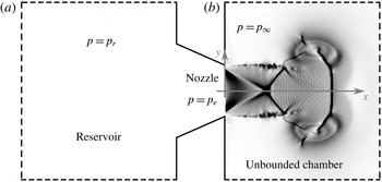
The basic configuration considered here for a compressible starting jet is a pressurised reservoir separated from an unbounded chamber by a convergent nozzle through which the fluid is discharged. The conditions in the reservoir are denoted with a subscript ‘
 $r$
’ (
 $p_{r}$
), while the conditions in the unbounded chamber are denoted with a subscript ‘
 $\infty$
’ (
 $p_{\infty }$
). The physical process starts when the pressure of the reservoir is released. In this moment a spherical compression wave travels into the unbounded chamber while an expansion wave travels inside the nozzle. After the initial compression wave, a vortex ring is generated at the lip of the nozzle. When the vortex ring is fully generated, the vortex ring propagates. A trailing jet might be generated after the vortex ring, depending on the injected mass supply. If the pressure ratio between the reservoir
 $p_{r}$
and the unbounded chamber
 $p_{\infty }$
(
 $p_{r}/p_{\infty }$
), hereafter called reservoir to ambient pressure ratio, is sufficiently high, the trailing jet can be supersonic, containing shock waves (§ 4.2). Depending on the size of the reservoir, here indicated as
 $L/D$
, the pressure will exponentially decay faster or slower. Here
 $L$
is the length of the reservoir assuming a cylindrical shape and
 $D$
is the nozzle exit diameter. The process ends when the reservoir and the unbounded chamber have the same pressure, assuming that the temperature difference does not play a role.
Experimenting with a buoyant plume, Turner (Reference Turner1962) developed the first model of the starting jet composed of a spherical vortex followed by a steady jet and found that the tip of the spherical vortex moves at approximately half of the maximum velocity in the jet at the same location for a later time. In a similar manner, reporting for incompressible flows experimentally, Witze (Reference Witze1980, Reference Witze1983) proposed a theoretical model that assumes the transient jet as a spherical vortex interacting with a steady jet and demonstrated that the ratio of the nozzle diameter (
 $D$
) to the jet velocity (
 $U$
) defines a time constant
 $\unicode[STIX]{x1D70F}=D/U$
that uniquely characterises the behaviour of impulsively started jets, leading to the dimensionless time
 $t^{\ast }=t/(D/U)$
. Recently, Gao & Yu (Reference Gao, Yu, New and Yu2015) reviewed the basic ideas on the incompressible starting jet and stated that the two broad directions of research are (i) the vortex ring pinch-off and (ii) entrainment enhancement in the pulsed jet propulsion systems.
Starting jets have been typically used in most of the experimental work to produce vortex rings, however the latter is the focus of the current research. Based on experimental observations, Maxworthy (Reference Maxworthy1972) described the flow field, the vortex ring’s velocity and the growth rate for stable rings. The reviews of Shariff & Leonard (Reference Shariff and Leonard1992) and Lim & Nickels (Reference Lim, Nickels and Green1995) provide a detailed background of vortex ring properties and its dynamics. In the literature, most of the experimental studies generate the vortex rings by ejecting an incompressible fluid moving a piston inside a cylindrical tube of diameter
 $D$
for a length
 $L$
into an open chamber, giving rise to the definition of the non-dimensional mass supply. The mass contained in a cylinder of diameter
 $D$
and length
 $L$
(
 $m_{cyl,L}$
), compared to the one contained in a cylinder with
 $L=D$
(
 $m_{cyl,L=D}$
), can be considered as the non-dimensional mass supply:
 $$\begin{eqnarray}\frac{m_{cyl,L}}{m_{cyl,L=D}}=\frac{\unicode[STIX]{x03C0}\left({\displaystyle \frac{D}{2}}\right)^{2}L\unicode[STIX]{x1D70C}}{\unicode[STIX]{x03C0}\left({\displaystyle \frac{D}{2}}\right)^{2}D\unicode[STIX]{x1D70C}}=\frac{L}{D}.\end{eqnarray}$$
At the very beginning of the process the axial and radial positions of the vortex ring (
 $x_{VR}$
and
 $r_{VR}$
, respectively) vary with
 $x_{VR}/D\sim (t^{\ast })^{3/2}$
and
 $r_{VR}/D\sim (t^{\ast })^{2/3}$
, for
 $0.1<t^{\ast }<1$
(Didden Reference Didden1979). At a later stage, for
 $t^{\ast }>1$
, the variation of the axial and radial positions of the vortex ring were found to be
 $x_{VR}/D\sim (t^{\ast })^{1/2}$
Witze (Reference Witze1980) and
 $r_{VR}/D\sim (t^{\ast })^{1/3}$
(Kelvin Reference Kelvin1867), respectively. Gharib, Rambod & Shariff (Reference Gharib, Rambod and Shariff1998) termed ‘formation time’ the dimensionless time
 $t^{\ast }=t/(D/U)$
and found a limiting value for the non-dimensional mass supply
 $(L/D)_{lim}$
of approximately four that universally defines the existence of a trailing jet after the vortex ring. This limiting value was called the ‘formation number’. These results were reproduced by Rosenfeld, Rambod & Gharib (Reference Rosenfeld, Rambod and Gharib1998) and many others but it was reported that this limiting value is not universal and it may vary within the range
 $1<(L/D)_{lim}<5$
depending on the spatial and temporal distribution of the inlet condition or Reynolds number (Rosenfeld et al.
Reference Rosenfeld, Rambod and Gharib1998; Zhao, Frankel & Mongeau Reference Zhao, Frankel and Mongeau2000; Gao & Yu Reference Gao and Yu2010). Hermanson, Dugnani & Johari (Reference Hermanson, Dugnani and Johari2000) defined the limiting parameter as
 $(L/D)_{lim}^{1/3}$
in order to be able to relate it to the characteristic length of a cylinder defined by the authors as the cubic root of the injected volume (
 $V_{0}^{1/3}$
), resulting in
 $(L/D)_{lim}^{1/3}\sim V_{0}^{1/3}/D$
.
The numerical studies related to this work have been typically focused on the vortex ring, because of the relatively low requirements of computational resources. The most closely related previous studies are presented here.
James & Madnia (Reference James and Madnia1996) studied the effect of different inlet velocity temporal distributions on the dynamics of the ring itself and found that during the formation phase of the ring, the impulse and the total circulation are approximately the same by generating the vortex ring through an orifice in a wall or through a nozzle, where no wall is around the lip of the nozzle.
Investigating the trailing jet instabilities numerically, Zhao et al. (Reference Zhao, Frankel and Mongeau2000) found that the pinch-off process, defined as the physical separation of the vortex ring from the trailing jet, is driven by the Kelvin–Helmholtz instabilities from the shear layer.
Archer, Thomas & Coleman (Reference Archer, Thomas and Coleman2008) focused on the vorticity distribution of thin- and thick-core vortex rings. Thin- and thick-core vortex rings were exemplified by the authors as
 $\unicode[STIX]{x1D6FF}/r_{VR}=0.2$
and
 $0.4$
, respectively, with
 $\unicode[STIX]{x1D6FF}$
the vortex ring core radius and
 $r_{VR}$
the vortex ring radius. While the diffusion of thin-core rings is well described by Saffman’s equation (Saffman Reference Saffman1970), the core diffusion of thick-core vortex rings is limited by the symmetry condition and the entrainment, with the vorticity distribution distorted.
Zaitsev, Kopiev & Kotova (Reference Zaitsev, Kopiev and Kotova2001) compared the noise measurements of a turbulent vortex ring with theory and confirmed that the turbulent vortex ring noise can be represented as the sum of three quadrupoles. The sound generation of a turbulent vortex ring consists of three stages (Ran & Colonius Reference Ran and Colonius2009): the instability waves which generate relatively weak sound, the vortex breakdown (connected with the maximum sound pressure level) and the turbulent decay, which leads to a decay in the sound pressure level (SPL) of 30 dB.
Concerning the jet flow, there exists a very extensive literature. Interested readers are directed to the review by Ball, Fellouah & Pollard (Reference Ball, Fellouah and Pollard2012), which provides a very clear and detailed overview of the different contributions. We present here a brief sketch of the jet flow research milestones.
Tollmien (Reference Tollmien1926), one of the first works in turbulent jets, considered an incompressible jet flow through Prandtl’s mixing length theory. The first experimental studies of a round jet were carried out by Ruden (Reference Ruden1933) and Kuethe (Reference Kuethe1935), who found that similarity of velocity profiles was reached before
 $10D$
. Today, the jet similarity and the region in which this takes place is still under debate. The first direct numerical simulation of a supersonic jet was reported by Freund, Lele & Moin (Reference Freund, Lele and Moin2000), who considered a jet with a Reynolds number
 $Re_{D}=2000$
based on the nozzle diameter and on the fully expanded Mach number
 $M_{j}=1.92$
at adapted conditions, focusing mainly on the confirmation of the direct numerical simulation and the acoustic radiated by the supersonic jet. As can be seen, the main focus until now has been to characterise the fluid flow through statistical analyses to obtain universal laws that define the behaviour of the jet flow.
The acoustic noise generated by the jet flow has been intensively studied since the 1950s, starting with Powell (Reference Powell1953), who considered the noise radiated by a choked nozzle flow. The jet noise, the acoustic noise generated by the continuous jet, especially the supersonic continuous jet, is a very useful reference for the acoustics of the compressible starting jet, which can be considered a new topic. A short overview of the closest jet noise references is presented here focusing on the supersonic case.
The reviews of Seiner & Yu (Reference Seiner and Yu1984) and Tam (Reference Tam1995) focus on the supersonic jet noise, providing a detailed discussion about the three different noise components and their generation. The turbulent mixing noise (TMN) is produced by the turbulent scales of the shear layer and therefore it is radiated in both subsonic and supersonic cases. The broadband shock noise (BBSN) is generated by the interaction between the shock waves and the vortices of the shear layer where the shock waves are reflected. The screech tones are generated by a feedback loop in which the acoustic waves travel backwards (in the subsonic surroundings of the jet) to the lip of the nozzle, triggering new disturbances that are again convected downstream until the point at which these acoustic waves were generated, where the shear layer vortices interact with the shock waves, closing in this way the loop with a specific frequency.
As typical in jet noise, the angle
 $\unicode[STIX]{x1D703}$
that characterises the directivity is measured from the jet axis in the upstream direction (Tam Reference Tam1995). Norum & Seiner (Reference Norum and Seiner1982) found that the directivity of BBSN is mainly in the upstream direction and that the BBSN shows a Doppler frequency shift with the measurement angle.
As proposed by Tam, Golebiowski & Seiner (Reference Tam, Golebiowski and Seiner1996), the TMN has two similarity spectra produced by two noise sources: (i) the large-scale similarity (LSS) spectrum produced by the large and coherent structures and (ii) the fine-scale similarity (FSS) spectrum produced by the fine turbulent scales. Some time later, Tam et al. (Reference Tam, Viswanathan, Ahuja and Panda2008) suggested that only two different sources of jet TMN exist: the fine-scale turbulence and the large turbulent structures of the jet flow. Comparing the noise of a perfectly expanded and an underexpanded jet from a convergent–divergent nozzle, Kim, Krejsa & Khavaran (Reference Kim, Krejsa and Khavaran1994) provided evidence that the presence of a shock cell structure does not modify the TMN.
The behaviour of the starting jet is governed by four main dimensionless parameters: the Reynolds number (
 $Re_{D}$
), affecting mainly the size of the Kelvin–Helmholtz instabilities relative to the nozzle diameter; the non-dimensional mass supply
 $(L/D)$
given by the length (
 $L$
) of a hypothetical cylindrical reservoir with a constant diameter (
 $D$
) (the same diameter as the nozzle) and the same volume than the real reservoir, influencing mainly the existence of a trailing jet, the reservoir to unbounded chamber pressure ratio (
 $p_{r}/p_{\infty }$
), having an effect on the compressibility and the reservoir to unbounded chamber temperature ratio
 $T_{r}/T_{\infty }$
.
The main objectives of this study are (i) to describe the physical phenomena involved in the compressible starting jet, (ii) to analyse the effects of the variation of the governing parameters, (iii) to define properly the pinch-off and (iv) to describe the interaction between the vortex ring and the trailing jet.
Until now, to the best knowledge of the authors, compressible starting jets have not been investigated.
The rest of the paper is organised as follows. Section 2 describes the system under study: the geometry chosen, the set of parameters and the assumptions that have been made. Section 3 deals with the method used to obtain the results, while the core of the article is § 4. The results are reported in four subsections, corresponding to the four main objectives explained in the introduction. Section 5 completes this work by drawing the conclusions.
2 Set-up description
We study a pressurised reservoir discharging fluid into an unbounded chamber at rest through a convergent nozzle, see figure 1. In a general manner, this process can be split in two main phases: (i) starts just after the release of the pressure, where we assume that the pressure of the reservoir is constant during the time in which the flow accelerates through the fully unsteady nozzle until a quasi-steady flow in the nozzle is reached. During this stage, the mass flow rate increases with time until the maximum of the inlet condition or until the nozzle is choked. In stage (ii), assuming quasi-steady flow through the nozzle, the pressure in the reservoir decreases with time until it reaches the pressure in the unbounded chamber. In the cases with supersonic flow, the second stage can be divided into (ii.a) during which the nozzle is choked and the mass flow rate is constant and (ii.b) during which the nozzle is no longer choked and the mass flow rate decreases with time, the flow being subsonic.
System set-up. The reservoir (a) is pressurised at
 $p_{r}$
and the fluid is injected through a convergent nozzle into the unbounded chamber (b), which has a pressure
 $p_{\infty }$
. The pressure at the centre of the nozzle exit is
 $p_{e}$
.

We restrict our analysis to the case
 $T_{r}=T_{\infty }$
, where
 $T_{\infty }$
is the temperature in the unbounded chamber. The inlet is chosen to be adiabatic and therefore an isentropic flow takes place from the reservoir up to the lip of the nozzle. Since the flow inside the nozzle is not computed, the variation of the inlet condition with the non-dimensional time (
 $t^{\ast }=t/(D_{j}/U_{j})$
, where
 $D_{j}$
and
 $U_{j}$
are the fully expanded diameter and velocity, respectively) is modelled as
 $$\begin{eqnarray}\left.\frac{p_{e}(t^{\ast })}{p_{\infty }}\right|_{y,z=0}=1+\frac{p_{r}/p_{\infty }}{\text{NPR}}\,\exp \left(\frac{-t^{\ast }}{C}\right)\tanh (Kt^{\ast }),\end{eqnarray}$$
where NPR is the nozzle pressure ratio, defined as the ratio reservoir total pressure to nozzle exit pressure
 $p_{r}/p_{e}$
. The one-dimensional isentropic theory predicts an exponential decay of the pressure in the deposit when discharging (Saad Reference Saad1985). We linked the initial state of quiescence with the exponential decay through a hyperbolic tangent. This is similar to the experimental work of Cimarelli et al. (Reference Cimarelli, Alatorre-Ibargengoitia, Kueppers, Scheu and Dingwell2014), where the pressure time distribution measured at the lip of the nozzle matches qualitatively with the model used in this study. If the nozzle is not choked (
 $M_{e}<1$
),
 $p_{e}=p_{\infty }$
because the flow in the nozzle is always adapted to the unbounded chamber conditions in the subsonic regime. However, if a convergent nozzle is choked (
 $M_{e}=1$
), NPR
 $^{\ast }=\left((\unicode[STIX]{x1D6FE}+1)/2\right)^{(\unicode[STIX]{x1D6FE}/(\unicode[STIX]{x1D6FE}-1))}$
(Becker Reference Becker1968) and
 $p_{e}\neq p_{\infty }$
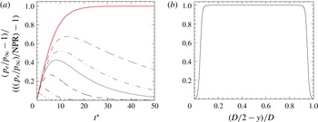
, because the flow in a convergent nozzle in supersonic regime is never adapted. Equation (2.1) is plotted in figure 2(a). The constant
 $K$
modifies the hyperbolic tangent term, which is responsible for the impulsive stage, corresponding to stage (i). The larger the value of
 $K$
, the more impulsive is the first stage. We used
 $K=60$
. In the same way, the constant
 $C$
modifies the exponential term, which is responsible for the decay, corresponding to stage (ii). The larger the value of
 $C$
, the faster is the decay, which also implies a smaller volume of the reservoir.
Nozzle exit conditions for the starting jet. (a) Pressure temporal distribution at the nozzle exit centreline for cases 1 to 7 (curves from bottom to top, see table 1). Note that the lines for cases 7.a, 7.b and 7.c collapse into the red line. (b) Pressure distribution at the nozzle exit plane for the case
 $7.a$
for
 $t^{\ast }=50$
.

The spatial pressure distribution imposed at the inlet (
 $p_{e}(y,z)/p_{\infty }$
), shown in figure 2(b), was modelled by,
 $$\begin{eqnarray}\left.\frac{p_{e}(y,z)}{p_{\infty }}\right|_{t_{0}}=1+\left(\frac{p_{r}/p_{\infty }}{\text{NPR}}-1\right)\left\{\frac{1}{2}-\frac{1}{2}\left[\tanh \left(\frac{\sqrt{y^{2}+z^{2}}-\frac{1}{2}(D-\unicode[STIX]{x1D6FF}_{\unicode[STIX]{x1D714}_{0}})}{l_{mass}}\right)\right]\right\},\end{eqnarray}$$
with a shear layer thickness of
 $\unicode[STIX]{x1D6FF}_{\unicode[STIX]{x1D714}_{0}}=0.1D$
. The most common spatial distribution of the inlet condition when numerically simulating a jet is a hyperbolic tangent, due to the good control over the gradients of the distribution to generate unstable Kelvin–Helmholtz vortices. We used this distribution as well, adding the unsteady part to take into account the time evolution of the inlet condition. This, together with a relatively large Reynolds number, led to a fully turbulent shear layer shortly after the nozzle exit. The parameter
 $l_{mass}=\unicode[STIX]{x1D6FF}_{\unicode[STIX]{x1D714}_{0}}/(2\unicode[STIX]{x03C0})$
controls the position of the shear layer in the nozzle, imposing the beginning of the shear layer at the wall and not centred into the wall.
In order to compare the results obtained in this study with those in the literature, we show in the following discussion the analogy between the main non-dimensional parameters of the cylinder–piston device typically used in the literature in the incompressible case with the discharge of a pressurised reservoir in the current study. To make this analogy we assume that the reservoir has a cylindrical form with the same diameter as the nozzle (
 $D$
) in which the unknown variable is the length (
 $L$
) of this hypothetical reservoir. By applying the continuity equation and integrating the mass injected (
 $m_{injected}$
) into the unbounded chamber with the help of the temporal and spatial inlet condition distributions, equations (2.1) and (2.2), respectively, we compute the mass supplied through the nozzle and therefore the length of the hypothetical reservoir that would have supplied the same mass. In other words, using the continuity equation, the mass contained in the unknown reservoir at high pressure (
 $m_{cyl,0}$
) is equal to the injected mass plus the mass contained in the reservoir at low pressure after the discharge (
 $m_{cyl,f}$
),
 $$\begin{eqnarray}m_{cyl,0}=m_{injected}+m_{cyl,f}.\end{eqnarray}$$
By integrating and manipulating algebraically the different terms in (2.3) and
 $$\begin{eqnarray}m_{injected}=\int _{0}^{\infty }\int _{-D/2}^{D/2}\int _{-D/2}^{D/2}\unicode[STIX]{x1D70C}(y,z,t)u(y,z,t)\,\text{d}z\,\text{d}y\,\text{d}t,\end{eqnarray}$$
we can express the non-dimensional mass supply (
 $L/D$
) as a function of the inlet condition parameters (
 $C,~K,~p_{r}/p_{\infty }$
),
 $$\begin{eqnarray}\displaystyle \displaystyle \frac{L}{D} & = & \displaystyle \frac{4RT_{r}}{\unicode[STIX]{x03C0}D^{3}}\frac{p_{\infty }^{1-\unicode[STIX]{x1D6FE}/\unicode[STIX]{x1D6FE}}\text{e}^{-s_{e}/c_{p}}c_{e}}{{\displaystyle \frac{p_{r}}{p_{\infty }}}-1}\sqrt{\frac{2}{\unicode[STIX]{x1D6FE}-1}}\nonumber\\ \displaystyle & & \displaystyle \displaystyle \times ~\int _{0}^{\infty }\int _{-D/2}^{D/2}\int _{-D/2}^{D/2}\sqrt{\left(\frac{p_{r}/p_{\infty }}{\text{NPR}}\right)^{\unicode[STIX]{x1D6FE}-1/\unicode[STIX]{x1D6FE}}-1}~\left(\frac{p_{r}/p_{\infty }}{\text{NPR}}\right)^{1/\unicode[STIX]{x1D6FE}}\,\text{d}y\,\text{d}z\,\text{d}t^{\ast }.\end{eqnarray}$$
Here
 $R$
denotes the specific gas constant,
 $T_{r}$
the temperature of the reservoir,
 $s_{e}$
the entropy at the nozzle exit,
 $c_{p}$
the heat capacity at constant pressure and
 $c_{e}$
the speed of sound at the nozzle exit.
Ricou & Spalding (Reference Ricou and Spalding1961) suggested that the entrainment coefficient does not vary in turbulent jets for Reynolds number larger than
 $10\,000$
and this value might be the start of the Reynolds independence regime for turbulent jets. Based on the relative magnitude of dimensional spatial scales, Dimotakis (Reference Dimotakis2000) reported that the fully developed turbulent flow requires an outer scale Reynolds number of
 $Re_{D}\gtrsim 10\,000$
–20 000. With these arguments, and with the limitations of computational capacity, we chose a Reynolds number of
 $10\,000$
for the starting jet without decay, case
 $7.b$
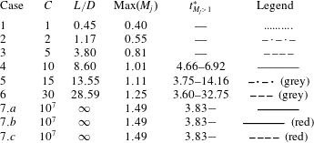
in table 1. To effectively simulate different starting jets, a
 $Re_{D}=5000$
was chosen for cases 1 to 6 as well as
 $7.a$
and
 $7.c$
, so that the grid requirements are not unpractical to perform a parameter variation.
Summary of the different cases and the involved parameters for
 $p_{r}/p_{\infty }=3.60$
. The supersonic non-dimensional time interval is represented with
 $t_{M_{j}>1}^{\ast }$
.

3 Numerical method
In the numerical code used, the three-dimensional compressible Navier–Stokes equations are formulated in the characteristic form as in Sesterhenn (Reference Sesterhenn2000). This formulation has several advantages, such as the straightforward implementation of non-reflecting boundary conditions for aeroacoustic applications and the use of upwind and downwind schemes to discretise the upwind and downwind waves, respectively.
The hyperbolic part of the Navier–Stokes equations is discretised with the compact upwind low dissipation fifth-order scheme of Adams & Shariff (Reference Adams and Shariff1996). The heat flux and friction terms are discretised with a sixth-order compact finite differences with spectral-like resolution. For time integration, a fourth-order Runge–Kutta with an explicit
 $\text{CFL}$
number is used, leading to a time step size of
 $\text{d}t=1.545\times 10^{-5}~\text{s}$
for the large resolution and
 $2.788\times 10^{-5}~\text{s}$
for the low resolution.
Since our interest is mainly focused on turbulence and acoustics, the strongest requirement for the computational grid in our direct numerical simulations (DNS) is to resolve the smallest turbulent scales present in the flow field. As a consequence, the smallest resolved acoustic wavelengths are the same size as the Kolmogorov length. The Cartesian geometry of length
 $25D\times 15D\times 15D$
was chosen to be discretised with
 $2048\times 1024\times 1024$
grid points for the cases
 $7.b$
(with
 $Re_{D}=10~000$
) and
 $7.c$
(with
 $Re_{D}=5000$
highly resolved). The resolution
 $512\times 256\times 256$
was chosen for the remaining cases. Both transverse directions have been discretised using a grid stretching, as proposed by Anderson, Tannehill & Pletcher (Reference Anderson, Tannehill and Pletcher1984), but in the axial direction the grid is equidistant.
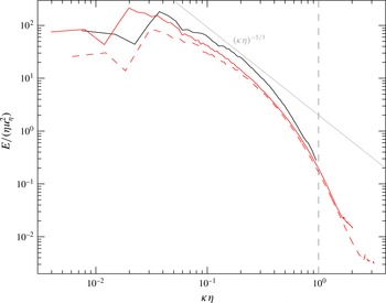
Non-dimensional turbulent kinetic energy spectra for the cases
 $7.a,7.b$
and
 $7.c$
. Legend as in table 1. The grey dashed line represents the wavenumber associated with the Kolmogorov scale. As a reference, the
 $-5/3$
decay line has been plotted in light grey.

The resolution chosen for all simulations is sufficient to resolve the Kolmogorov scale, see figure 3. The turbulent spectra were calculated using the velocity fluctuations with respect to the azimuthal average:
 $u^{\prime }=u-\overline{u}_{\unicode[STIX]{x1D703}}$
, where
 $u$
is the instantaneous velocity and
 $\overline{u}_{\unicode[STIX]{x1D703}}$
is the mean velocity averaged in the azimuthal direction. This is supported and extended in table 2. The minimum value of the Kolmogorov length scale
 $\unicode[STIX]{x1D702}_{min}$
compared to the grid characteristic length is very close to one in the worst case (
 $7.a$
). The Kolmogorov length scale (calculated as
 $\unicode[STIX]{x1D702}=(\unicode[STIX]{x1D708}^{3}/\unicode[STIX]{x1D700})^{1/4}$
, where
 $\unicode[STIX]{x1D700}=\unicode[STIX]{x1D708}\langle \unicode[STIX]{x2202}u_{i}^{\prime }/\unicode[STIX]{x2202}x_{j}\unicode[STIX]{x2202}u_{i}^{\prime }/\unicode[STIX]{x2202}x_{j}\rangle$
) is time dependent and decreases with the starting phase, while it increases during the decay phase. Both continuous cases with
 $Re_{D}=5000$
(cases
 $7.a$
and
 $7.c$
) have a very good agreement in the inertial subrange and the beginning of the dissipation range. Only few points are in the energy containing scales and since the data are not time averaged, the agreement appears to be satisfactory. Comparing both spectra corresponding to the high resolution (
 $2048\times 1024\times 1024$
) we find an excellent agreement in the dissipation range as well as in the inertial subrange. The spectra of case
 $7.b$
corresponding to
 $Re_{D}=10\,000$
has a longer inertial subrange and there is more energy associated with large scales, as expected. All spectra present a small peak for high wavenumbers, which corresponds to the error associated with the interpolation to an equidistant grid to perform the Fourier transformation. Figure 3 shows the energy spectra for the continuous jets with different resolutions, showing the worst scenario in terms of
 $\unicode[STIX]{x1D702}_{min}/\text{d}_{grid}$
; for the starting–decaying jets with the same governing parameters but for
 $L/D$
, the lower Mach numbers make the Kolmogorov length scale increase, leading to less critical conditions for the numerical grid.
Grid spacing considerations for the cases under study. The characteristic length of the smallest element in the domain is defined as
 $\text{d}_{grid}=\left(\text{d}x_{min}+\text{d}y_{min}+\text{d}z_{min}\right)/3$
where
 $\unicode[STIX]{x1D702}_{min}$
is the minimum Kolmogorov length scale and
 $\unicode[STIX]{x1D708}_{\infty }=\unicode[STIX]{x1D708}(T_{\infty })$
is the kinematic viscosity at the temperature of the unbounded chamber in
 $\text{m}^{2}~\text{s}^{-1}$
.

The numerical code is parallelised with a hybrid approach message passing interface (MPI)/OpenMP. More details are given in Schulze (Reference Schulze2011). Up to
 $8192$
CPUs were used.
Non-reflecting boundary conditions were imposed in all four lateral boundaries, while a sponge region was imposed at the outlet. The inlet conditions were described in the set-up description, see § 2. Quiescent conditions were imposed as the initial condition.
The width of an inviscid shock wave is approximately one order of magnitude larger than the mean free path (Salas & Iollo Reference Salas and Iollo1996). Using non-dimensional analysis, the Knudsen number can be expressed in the form
 $Kn=\unicode[STIX]{x1D706}/D=M_{j}\sqrt{\unicode[STIX]{x1D6FE}\unicode[STIX]{x03C0}/2}/Re$
and since the characteristic length in this study (the nozzle diameter,
 $D$
) is chosen to be unity, the mean free path (
 $\unicode[STIX]{x1D706}$
) – and therefore the thickness of the shock waves (
 $10\unicode[STIX]{x1D706}$
)– is much smaller than the grid elements (
 $10\unicode[STIX]{x1D706}/d_{grid}$
in table 2). We used the shock capturing filter from Bogey, de Caqueray & Bailly (Reference Bogey, de Caqueray and Bailly2009).
4 Results and discussion
In this section the results of the study are presented divided in four subsections, corresponding to the main objectives of this article.
4.1 Description of the involved physical phenomena
Stages of the starting jet. Numerical schlierens (
 $|\unicode[STIX]{x1D735}\unicode[STIX]{x1D70C}|$
) are shown. The case
 $7.b$
is represented in (a) for
 $t^{\ast }=0.8$
, (b)
 $t^{\ast }=3.2$
and (c)
 $t^{\ast }=5.9$
and case
 $6$
is represented in (d) for
 $t^{\ast }=72$
.

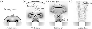
During the impulsive discharge of the reservoir, just after the release of the pressure through the nozzle, a compression wave is formed. This compression wave is generated by the sudden expansion at the lip of the nozzle due to the impulsive start. The compression wave has a half-spherical form and travels into the unbounded chamber with the speed of sound if it is a pressure wave, as in figure 4(a), or faster if it is a blast wave (Taylor Reference Taylor1950).
During the propagation of the pressure wave in the first few diameters, a vortex ring is always generated due to the large velocity gradients, figure 4(b). The vortex ring grows until a critical size is reached (
 $1.08D$
proposed by Didden Reference Didden1979) and then it starts propagating in the axial direction. Shortly after the beginning of the vortex ring propagation, the vortex ring separates from the trailing jet (if existing) and propagates further, detached from the rest of the flow. This separation process is called ‘pinch-off’ and it is ideally defined as the lack of vorticity between the vortex ring and the trailing jet, although this is a very strong criterion because in turbulent flows there is no lack of vorticity between the vortex ring and the trailing jet. Instead of the lack of vorticity, we propose to establish a vorticity threshold (
 $\unicode[STIX]{x1D714}_{po}$
) to define the pinch-off. A detailed analysis deals with this threshold in § 4.3.1, leading to the conclusion that the best definition of the pinch-off is the separation of the vortex ring and the trailing jet for the first time by a vorticity value
 $\unicode[STIX]{x1D714}_{po}$
relative to the maximum vorticity in the vortex ring (
 $\unicode[STIX]{x1D714}_{vortex}$
) of
 $\unicode[STIX]{x1D714}_{po}/\unicode[STIX]{x1D714}_{vortex}=0.1$
. In order to predict the pinch-off, a relationship between the normalised circulation injected until the pinch-off and the non-dimensional time is provided in § 4.3.2.
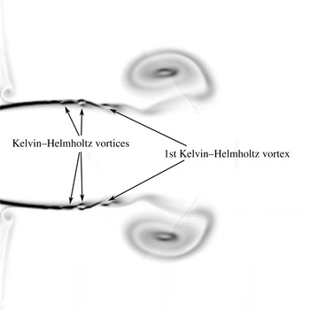
The pinch-off process is driven by the Kelvin–Helmholtz instabilities from the shear layer in the trailing jet (Zhao et al. Reference Zhao, Frankel and Mongeau2000). When the successive Kelvin–Helmholtz vortices in the shear layer are generated, they start rotating and drawing in vorticity from upstream and downstream of the vortex in the shear layer and this leads to a vorticity distribution along the shear layer with concentrated regions of large vorticity (the vortices) separated by regions of relatively low vorticity (the spaces between two consecutive vortices). These spaces between vortices are the potential points where the pinch-off would take place, see figure 5. The first Kelvin–Helmholtz vortex after the vortex ring is the first which is generated and therefore the one which will create the first a region of very low vorticity around it (if it is not ingested by the head vortex ring), leading to the pinch-off when the low vorticity reaches the pinch-off criterion (in this study defined in § 4.3.1). The dynamics of the shear layer vortices plays a crucial role in the pinch-off process.
Flow configuration for
 $t^{\ast }=5.5$
showing the development of the Kelvin–Helmholtz vortices in the case
 $7.b$
. The vorticity magnitude is shown in a black and white colour scale.

In the case of the existence of a trailing jet, the jet interacts with the vortex ring for large values of the Reynolds number. This interaction, here called shock–shear layer–vortex ring interaction, is explained in detail in § 4.4, leading to one of the loudest noise sources of the starting jet and comparable to those of the continuous jet.
The trailing jet can be subsonic during the whole process or supersonic during the impulsive period and subsonic during the final decay, (see figure 4 d), but it cannot be subsonic during the first stage, followed by a supersonic stage and a final subsonic decay because we focus on the impulsively starting jet: the acceleration time interval to have supersonic flow at the nozzle exit should be shorter than the time in which the vortex ring is completely generated, so in the onset of the trailing jet there are already supersonic conditions. Since the pressure at the inlet changes continuously with time, the jet will be adapted for a specific time (when the pressure ratio is the one the nozzle was designed for), being imperfectly expanded for the rest, which means that the supersonic associated phenomena such as shock waves and expansion fans will be present for most of the supersonic stage. Also due to the evolution of the inlet condition during the decay phase, the shock waves present in the trailing jet translate with a specific velocity, comparable to the speed of sound, having a strong effect on the acoustic radiated. More details are given in § 4.4.3.
The noise radiation directionality of the continuous jet is very well known in the community. In § 4.4.4 we study the angular dependence of the sound pressure level for the starting jet and compare it with the continuous one.
The physical process finishes when the reservoir reaches the pressure of the unbounded chamber, assuming that the effects of buoyancy or mass diffusion due to temperature differences between the reservoir and the unbounded chamber can be neglected.
4.2 Effects of the variation of the governing parameters
In this subsection we address the questions of what changes take place in the physical phenomena of the compressible starting jet when changing the governing parameters and what are the limiting values of the governing parameters that define a specific behaviour.
4.2.1 Reynolds number (
 $Re_{D}$
)

The main effect of the Reynolds number in the starting jet is the size of the Kelvin–Helmholtz instabilities in the shear layer of the trailing jet compared to the nozzle diameter. A larger Reynolds number leads to a smaller size of instabilities, and vice versa. We observed that a smaller size of the Kelvin–Helmholtz instabilities leads to an earlier pinch-off. The smaller vortices are earlier formed in the jet and they start earlier to absorb vorticity upstream and downstream of the vortex which leads to a situation in which the vorticity threshold defined for the pinch-off is reached earlier. Therefore, there is a critical Reynolds number (
 $Re_{D,interaction}$
) that makes the first Kelvin–Helmholtz vortex to be already formed when it passes through the first shock wave, see figures 4(c) and 5. Only if the Reynolds number is larger than this critical value will the shock–shear layer–vortex interaction take place. The Reynolds numbers in this study (
 $Re_{D}=5000$
and
 $10\,000$
) exceed this critical value, but the Reynolds number in Zhao et al. (Reference Zhao, Frankel and Mongeau2000), (
 $Re_{D}=3800$
) is clearly under the critical one. The critical Reynolds number
 $Re_{D,interaction}$
for the shock–shear layer–vortex interaction is an open question and future work should answer this question. For more details see § 4.4.
Studying the conditions that are needed to generate an incompressible laminar vortex ring, a laminar vortex ring that transitions to turbulence and an initially turbulent vortex ring, Glezer (Reference Glezer1988) generated a map, specifying that for Reynolds numbers (defined as
 $\unicode[STIX]{x1D6E4}/\unicode[STIX]{x1D708}$
) larger than
 $2.5\times 10^{4}$
an initially turbulent vortex ring was generated. For laminar-generated vortex rings, an azimuthal instability (similar in appearance to the Kelvin–Helmholtz instability of a free shear layer) amplifies and makes the vortex ring breakdown to turbulence. It was also reported by the authors that for larger velocities at the nozzle exit, the axial distance to the turbulent transition of the vortex ring was shorter. This interaction is hereafter called shear layer–vortex interaction. We observed that compressibility accelerates the onset of this interaction.
4.2.2 Dimensionless mass supply (
$L/D$
)

As already shown in the introduction,
 $L/D$
can be defined as the dimensionless mass supply, equation (1.1). Alternatively, this parameter might also be seen as a non-dimensional volume to be ejected by the nozzle.
The limiting value of the non-dimensional mass supply
 $(L/D)_{lim}$
dictates the existence of a trailing jet after the vortex ring in the starting jet. The more mass is injected by the nozzle, the more vorticity is provided to the vortex ring. If the vortex ring takes all the vorticity ejected by the nozzle we call it not saturated, because it could take more vorticity. If the vortex ring does not take all the vorticity ejected by the nozzle, a trailing jet is generated with the rest of the vorticity that the vortex ring is not able to take. In this case the vortex ring is saturated. A limit has been already been set for the value of
 $L/D$
to saturate the vortex ring (Gharib et al.
Reference Gharib, Rambod and Shariff1998),
 $(L/D)_{lim}\simeq 3.6$
–4.5, but it has been stated that this limit is not universal and it depends on the temporal and spatial inlet condition distributions, as well as the Reynolds number (Rosenfeld et al.
Reference Rosenfeld, Rambod and Gharib1998; Zhao et al.
Reference Zhao, Frankel and Mongeau2000; Gao & Yu Reference Gao and Yu2010). More details are given in § 4.3.2. The limiting value
 $(L/D)_{lim}$
for compressible flows is an open question that should be addressed by future work, but from observations in this study the value appears to be very close to the incompressible one.
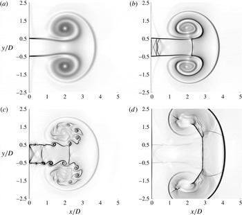
Starting jet fluid flow with different sets of parameters of several two-dimensional simulations to exemplify the differences not only between the incompressible and the compressible cases, but also among the compressible cases for different regimes: (a) incompressible, (b) supersonic laminar, (c) supersonic turbulent, (d) supersonic with blast wave. The axial position of the vortex ring is
 $x_{VR}/D=2$
for all cases. (a)
 $p_{r}/p_{\infty }=1.007$
,
 $L/D\rightarrow \infty$
,
 $Re=5000$
,
 $T_{r}/T_{\infty }=1$
.
 $t^{\ast }=6.41$
.
 $M_{j}=0.1$
.
 $\unicode[STIX]{x1D735}\unicode[STIX]{x1D70C}\in [0,0.025]$
. (b)
 $p_{r}/p_{\infty }=3.79$
,
 $L/D=8$
,
 $Re=5000$
,
 $T_{r}/T_{\infty }=1$
.
 $t^{\ast }=13.37$
.
 $M_{j}=1.27$
.
 $\unicode[STIX]{x1D735}\unicode[STIX]{x1D70C}\in [0,2]$
. (c)
 $p_{r}/p_{\infty }=2.84$
,
 $L/D\rightarrow \infty$
,
 $Re=5000$
,
 $T_{r}/T_{\infty }=1$
.
 $t^{\ast }=12.72$
.
 $M_{j}=1.32$
.
 $\unicode[STIX]{x1D735}\unicode[STIX]{x1D70C}\in [0,3]$
. (d)
 $p_{r}/p_{\infty }=50$
,
 $L/D=0.17$
,
 $Re=5000$
,
 $T_{r}/T_{\infty }=1$
.
 $t^{\ast }=6.91$
.
 $M_{j}=1.70$
.
 $\unicode[STIX]{x1D735}\unicode[STIX]{x1D70C}\in [0,4]$
.

The starting jet with a finite
 $L/D$
will not reach the same maximum fully expanded Mach number expected for the continuous jet (
 $L/D\rightarrow \infty$
) at the same pressure ratio (
 $p_{r}/p_{\infty }$
). The maximum fully expanded Mach number decreases with lower
 $L/D$
values. After the release of the pressure, the expansion wave that travels inside the nozzle is reflected at the bottom of the reservoir for an earlier time, so the expansion takes place during a shorter period.
The stability of the shear layer might also be influenced by this parameter. On the one hand, the jet in figure 6(c) shows an unstable shear layer. This jet comes from an infinite reservoir (
 $L/D\rightarrow \infty$
), blowing continuously and the combination of the governing parameters lead to an unstable shear layer and a turbulent jet. On the other hand, the jet in figure 6(b) shows a stable shear layer. This jet comes from a finite reservoir (
 $L/D=8$
) and is already in the decay stage, so it does not blow with the maximum velocity and the shock waves are travelling towards the nozzle exit. However, the leading vortex ring is propagated in the axial direction. This leads to a stable shear layer and a laminar jet.
4.2.3 Pressure ratio (
$p_{r}/p_{\infty }$
)

The steady fully expanded Mach number of a continuous jet can be determined just by
 $p_{r}/p_{\infty }$
, assuming
 $\unicode[STIX]{x1D6FE}=1.4$
for diatomic gases, by using the one-dimensional isentropic theory. The larger is
 $p_{r}/p_{\infty }$
the stronger is the expansion through the nozzle and the larger is the fully expanded Mach number. In the compressible starting jet,
 $p_{r}/p_{\infty }$
plays a crucial role determining the existence of shock waves, expansion fans and other supersonic phenomena. This parameter does not play a role in the incompressible case.
The minimum reservoir to unbounded chamber pressure ratio needed to chock a one-dimensional isentropic convergent nozzle is given by (e.g. Becker Reference Becker1968)
 $(p_{r}/p_{\infty })^{\ast }=((\unicode[STIX]{x1D6FE}+1)/2)^{(\unicode[STIX]{x1D6FE}/(\unicode[STIX]{x1D6FE}-1))}$
. The pressure ratio must reach this value to achieve supersonic flow. In this case is still possible to have a compressible starting jet where the different elements interact with each other creating a unified motion, but we focus on the supersonic case.
In this case, only in the time interval with supersonic flow, the acoustic components associated with supersonic flow – mainly broadband shock noise – will be radiated. Due to the time-dependent nozzle exit pressure ratio and the fixed geometry, the flow is imperfectly expanded. This leads to the existence of the supersonic phenomena and the corresponding acoustic components.
Ishii et al. (Reference Ishii, Fujimoto, Hatta and Umeda1999) found by applying the Rankine–Hugoniot relations across a moving shock that the required pressure ratio to generate a blast wave is
 $(p_{r}/p_{\infty })_{blast}=41.2$
. An example of a set-up with a blast wave is shown in figure 6(d). In this study the typical values for
 $p_{r}/p_{\infty }$
are approximately
 $3.6$
and therefore only pressure waves are formed.
Didden (Reference Didden1979) proposed a critical size of a vortex ring (
 $r/D=1.08$
) at which it stops growing and starts propagating in the axial direction. For large values of
 $p_{r}/p_{\infty }$
, a Prandtl–Meyer expansion was observed, leading to a widening of the flow after the nozzle exit and therefore leading to larger vortex rings before propagation starts, see figure 6(d). For values of
 $p_{r}/p_{\infty }$
that lead to a supersonic flow the vortex ring has a shock wave in its front, so that the pressure of the supersonic flow inside the vortex ring is matched to the pressure ahead of the vortex ring. This is presented in figure 6(b–d).
4.2.4 Temperature ratio (
$T_{r}/T_{\infty }$
)

In this study we focused on the compressible starting jet where
 $T_{r}/T_{\infty }=1$
, but as already reported in the literature, a hotter jet can lead to a larger reduction of loudness in the high frequency content than in the lower frequency content, but the typical values investigated to have a significant impact in the acoustics are
 $T_{r}/T_{\infty }\sim 2$
, see Tam (Reference Tam1991) and Tanna (Reference Tanna1977a
,Reference Tanna
b
). Most of the reported results related to hot jets focus on the acoustics. Further work is needed in this direction.
4.3 Pinch-off definition
Pinch-off is ideally defined as the separation of the vortex ring from the rest of the fluid flow by a region of zero vorticity. In turbulent flows, due to vorticity diffusion, there is in fact no region with zero vorticity. In this subsection we discuss the relationship between the vorticity field and the pinch-off.
4.3.1 Pinch-off vorticity threshold (
$\unicode[STIX]{x1D714}_{po}/\unicode[STIX]{x1D714}_{vortex}$
)

We define the pinch-off as the separation of the vortex ring from the rest of the fluid flow by a vorticity threshold of
 $\unicode[STIX]{x1D714}_{po}/\unicode[STIX]{x1D714}_{vortex}$
. The vorticity in the vortex ring core is denoted by
 $\unicode[STIX]{x1D714}_{vortex}$
. Choosing a value for this threshold close to unity, we would estimate the pinch-off to occur during the formation of the vortex ring and choosing a value of exactly zero, we would imply that the vortex ring would be surrounded by a large region of almost zero vorticity, an estimated pinch-off not representative in either of the two cases. Moreover, the region of low vorticity has a flat distribution and the pinch-off definition is very sensitive to
 $\unicode[STIX]{x1D714}_{po}/\unicode[STIX]{x1D714}_{vortex}$
.
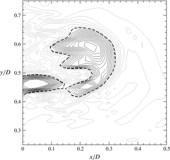
Sketch of the pinch-off vorticity threshold method. The black dashed line corresponds to the separation vorticity (
 $\unicode[STIX]{x1D714}_{s}/\unicode[STIX]{x1D714}_{vortex}=0.34$
). Higher values of vorticity (dark contour lines) define two separated regions, while lower values (light contour lines) define only one region. Results corresponding to case
 $7.a$
for
 $t^{\ast }=3.1$
.

Time evolution of the separation vorticity. See legend in table 1. The pinch-off vorticity threshold (
 $\unicode[STIX]{x1D714}_{s}/\unicode[STIX]{x1D714}_{vortex}=\unicode[STIX]{x1D714}_{po}/\unicode[STIX]{x1D714}_{vortex}=0.1$
) is denoted by (– – – –).

To choose the proper pinch-off vorticity threshold, we focus now on the limiting vorticity value that separates the vortex ring from the nozzle exit (or the trailing jet) and we call it the separation vorticity (
 $\unicode[STIX]{x1D714}_{s}$
). In other words, vortex ring and nozzle exit (or trailing jet) are separated by a region of vorticity with a value of at least
 $\unicode[STIX]{x1D714}_{s}$
. A lower value than
 $\unicode[STIX]{x1D714}_{s}$
defines only one region and cannot distinguish both regions, see figure 7.
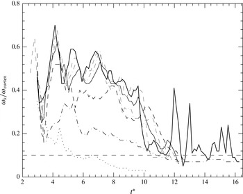
The relative separation vorticity (
 $\unicode[STIX]{x1D714}_{s}/\unicode[STIX]{x1D714}_{vortex}$
) decreases with time, see figure 8. The pinch-off takes place when this value reaches the pinch-off vorticity threshold (
 $\unicode[STIX]{x1D714}_{s}/\unicode[STIX]{x1D714}_{vortex}=\unicode[STIX]{x1D714}_{po}/\unicode[STIX]{x1D714}_{vortex}$
). We defined
 $\unicode[STIX]{x1D714}_{po}/\unicode[STIX]{x1D714}_{vortex}=0.1$
.
The relative separation vorticity shows a local minimum for all cases for
 $t^{\ast }\approx 3.4$
, as shown in figure 8. This is followed by different local maxima, which are due to vortices from the shear layer (compact regions with large vorticity values) that are taken in by the vortex ring. These vortices from the shear layer ‘rejoin’ the vortex ring with the trailing jet and separate them again when they are convected from the shear layer to the vortex ring. This process might be repeated for the few first Kelvin–Helmholtz vortices. This non-monotonic behaviour of the separation vorticity makes the definition of the pinch-off difficult. As an example, assuming
 $\unicode[STIX]{x1D714}_{po}/\unicode[STIX]{x1D714}_{vortex}=0.1$
, the pinch-off would take place multiple times (for
 $t^{\ast }=5.2$
and
 $6.5$
) for the case
 $1$
(
 $L/D=0.45$
). The pinch-off would take place also in a ‘multiple way’ for the rest of the cases in this study because the vorticity packages have even stronger peaks.
We therefore define the pinch-off as the first time that the vortex ring separates from the rest of the fluid flow taking as the pinch-off vorticity threshold
 $\unicode[STIX]{x1D714}_{po}/\unicode[STIX]{x1D714}_{vortex}=0.1$
.
For large Reynolds numbers, the pinch off takes place in a ‘multiple way’ because there are more Kelvin–Helmholtz vortices in the shear layer that are taken in by the vortex ring, leading to the peaks in the separation vorticity in figure 8. For low Reynolds numbers, the pinch-off takes place in a single way; the shear layer is stable and the separation vorticity decreases monotonically until the pinch-off vorticity threshold. There exists a critical Reynolds number that defines the boundary between the two types of pinch-off, as discussed in § 4.2. This is an open question that should be addressed by future research.
The separation vorticity presents a local minimum for all cases for
 $t^{\ast }\approx 3.4$
. This minimum can be interpreted as an interruption in the vortex ring generation, which introduces strong perturbations in the vortex ring that can lead to instabilities that grow and make the vortex ring transition to turbulent.
4.3.2 Circulation divergence law
By computing the circulation (
 $\unicode[STIX]{x1D6E4}$
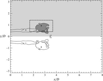
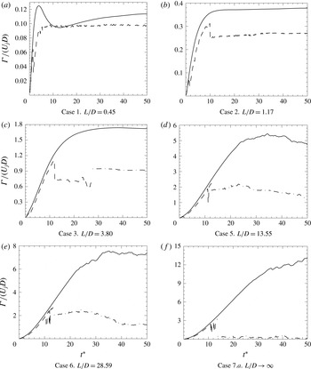
) in a semi-plane that contains the jet axis (hereafter called the sagittal semi-plane, shown as the light grey region in figure 9) and in the intersection of this semi-plane with the vortex ring (dark grey region in figure 9), we show that despite injecting more vorticity through the nozzle, from a certain point on, the vortex ring does not absorb any vorticity more, see figure 10.
For the cases with small
 $L/D$
(cases
 $1$
and
 $2$
), the entire circulation contained in the sagittal semi-plane was concentrated in the vortex ring and no trailing jet was formed, figure 10(a,b). The vortex ring absorbed the whole vorticity injected through the nozzle. We call this situation a non-saturated vortex ring. A trailing jet was not formed in cases
 $1$
and
 $2$
. The small difference between the circulation contained in the vortex ring and in the sagittal plane in figure 10(a) is due to the entrainment of fluid, generating a region of positive and negative vorticity close to the lip of the nozzle that decay at a different rate with time. This phenomenon takes place in the rest of the cases, but the amount of circulation generated due to the entrainment is small compared to the one in the vortex ring and may be neglected.
For the cases with large
 $L/D$
(cases
 $3$
,
 $4$
,
 $5$
,
 $6$
and
 $7$
), the qualitative behaviour was completely different. After some time, during the injection of the vorticity, the circulation contained in the vortex ring did not follow that contained in the sagittal semi-plane and the vortex ring did not absorb any additional vorticity, as seen in figures 10(c–f). We call this situation a saturated vortex ring. The ejected circulation not belonging to the vortex ring formed the trailing jet.
Sketch of the different methods used to compute the circulation. The light grey shaded area, defined here as the sagittal semi-plane, is a general semi-plane that contains the jet axis. The black star is the location of the vortex ring following the method proposed by Pawlak et al. (Reference Pawlak, Marugan Cruz, Martinez Bazan and Garcia Hrdy2007). The dark grey area corresponds to the vortex ring area identified by the flood-fill method centred in the vortex ring location and using as a boundary the contour line
 $\unicode[STIX]{x1D714}=0.1\unicode[STIX]{x1D714}_{vortex}$
(plotted here as a solid black line). For the cases with turbulent vortex ring the most stable method to compute the circulation of the vortex ring is a window of
 $2D\times 1D$
(plotted as a dashed black line) defined centred in the vortex ring location.

Circulation contained in the
 $x$
–
 $y$
sagittal semi plane (——) and the circulation contained in the intersection of this semi-plane with the vortex ring (- - - -) over the non-dimensional time by the flood fill method. Circulation contained in the intersection of the sagittal semi-plane with the vortex ring by the window method (– ⋅ – ⋅ –).

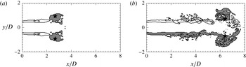
When integrating the vorticity in the intersection of the sagittal plane and the vortex ring, the identification of the integration domain was done by the flood fill method, see figure 9. While the vortex ring is laminar, or remains in low levels of turbulence, the vortex is very clear and both the identification and the integration of the vorticity are straightforward, see figure 11(a). When the vortex ring becomes turbulent, the region of high vorticity is not a simply connected space and changes drastically with time, which makes the integration much more difficult, see figure 11(b). This is the reason for the non-uniform behaviour of the vortex ring circulation (dashed line) in figure 10. When the vortex ring became turbulent and the circulation obtained was not representative, we integrated the vorticity following the most widespread method used in the literature: integrating the vorticity within a
 $2D\times 1D$
window, see figure 10. The transversal size of the window of
 $1D$
was chosen not to cross the jet axis when the leading vortex ring is generated, located at
 $r/D=0.5$
.
Vorticity contour for two different stages of case
 $7.b$
. The solid black line corresponds to
 $\unicode[STIX]{x1D714}_{po}/\unicode[STIX]{x1D714}_{vortex}=0.1$
. The dark grey region is the vortex ring as identified by the flood fill method. The vortex ring (following Pawlak et al.
Reference Pawlak, Marugan Cruz, Martinez Bazan and Garcia Hrdy2007) is denoted by (
 $\star$
). (a) Successful identication of the vortex ring. The integration of the vorticity within the dark grey domain leads to a proper circulation contained in the vortex ring.
 $t^{\ast }=12.5$
. (b) Unsuccessful identication of the vortex ring. The integration of the vorticity does not give us a proper circulation value because the upper half of the vortex has already been detached from the trailing jet but the lower half is still attached. Furthermore, due to turbulence, the vortex ring is not a simply connected space.
 $t^{\ast }=22$
.

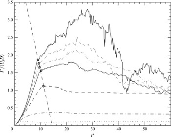
Vortex ring circulation over the non-dimensional time. The pinch-off is shown by the points (●) (grey) in which the circulation of the sagittal semi-plane and in the vortex ring diverged. A linear regression (- - - - - -) (grey) has been taken into consideration as the relationship that predicts the pinch-off. Lines as in table 1.

We can relate this to the pinch-off process: when the circulation in the vortex ring does not follow the one contained in the sagittal semi-plane, two different regions with relatively high vorticity were created. The divergence of these both curves determines the physical separation of the vortex ring. This divergence can be seen in the different cases in figure 10 as well as in figure 12. In order to predict the pinch-off, a relationship between the dimensionless time
 $(t^{\ast })$
and the Reynolds number for which the pinch-off takes place
 $(\unicode[STIX]{x1D6E4}/U_{j}D)_{pinch-off}$
was established, equation (4.1). Since all pinch-off points are over a straight line in figure 12, an empirical linear relationship was indicated as
 $$\begin{eqnarray}\left(\frac{\unicode[STIX]{x1D6E4}}{U_{j}D}\right)_{pinch-off}=5.0071-0.3467(t^{\ast }).\end{eqnarray}$$
4.4 Interaction between the vortex ring and the trailing jet
In both the starting and continuous stage of the jet there is an interaction between the vortices and the shock waves of the trailing jet, but both of these interactions take place in a slightly different way. In the starting stage, the vortex ring interacts with the shock waves and the vortices of the shear layer, while in the continuous stage, the shock waves interact with the vortices of the shear layer but not with the vortex ring. Both interactions generate two of the three loudest noise sources of the compressible starting jet.
4.4.1 Shock–shear layer–vortex interaction
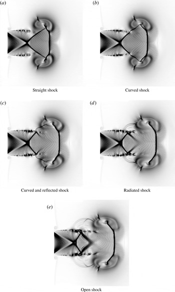
When the impulsively started jet is only few nozzle diameters long, the first shock wave extends until the vortex ring core, see figure 13(a). The vortices from the shear layer are convected to reach the shock wave, corresponding to the figure 13(b). In this point takes place the shock–shear layer–vortex interaction and the shock wave bends due to the vorticity of the shear layer.
When the first vortices of the shear layer pass through the shock wave, the velocity gradients of the shear layer bend the affected segment of the shock wave more and more, and the shock wave starts to be reflected in the shear layer, as shown in figure 13(c).
For later times, the segment of the shock wave between the shear layer and the vortex ring is radiated as a strong acoustic wave into the surroundings, figure 13(d,e).
Stages of the shock cell structure during its interaction with the vortex ring. The numerical schlierens
 $|\unicode[STIX]{x1D735}\unicode[STIX]{x1D70C}|$
are plotted in the range
 $\left[0,2\right]$
. Case
 $7.b$
is represented for (a)
 $t^{\ast }=5.1$
, (b)
 $t^{\ast }=5.6$
, (c)
 $t^{\ast }=5.9$
, (d)
 $t^{\ast }=6.3$
and (e)
 $t^{\ast }=6.8$
.

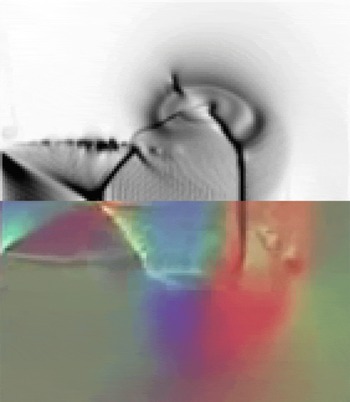
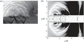
Lower half: time-resolved colour schlieren image from Kleine et al. (Reference Kleine, Le, Takehara and Etoh2010). Upper half: numerical schlieren corresponding to case
 $7.b$
.

Figure 14 compares visually an experimental schlieren image from Kleine et al. (Reference Kleine, Le, Takehara and Etoh2010), with a numerical image from case
 $7.b$
. The different structures and the shock–shear layer–vortex interaction can be identified at first sight in both images. The agreement is reasonable. The segment of the shock wave extended from the shear layer to the vortex ring is bent in the same way in both cases just before the sound radiation. Due to the resolution of the experimental image, the details of the leading vortex ring cannot be compared. There is also a region ahead of the vortex ring in which the experiment shows some vorticity content not reproduced in the numerical simulation. The rest of the visible structures are identical.
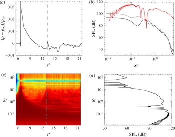
In order to show that this interaction generated a noise at least as loud as the loudest noise source of the continuous jet for the same parameters we placed a numerical probe at
 $5D$
from the jet axis. Pressure fluctuations of approximately
 $600$
Pa were recorded, figure 15(a). Taking the wavelet transformation (complex Morlet wavelet) of the recorded signal we analysed its frequency content as a function of time, see figure 15(c). The correspondence between the peak of the front pressure wave with the maxima of the coefficients for
 $t^{\ast }\approx 6.67$
is straightforward and the peak corresponding to the interaction is also easy to identify. The dashed line in figure 15(a,c) represents the time in which the noise generated by the interaction arrives at the numerical probe. The spectrum obtained through the wavelet transformation for the time of the interaction is presented in 15(b) (red) and 15(d), showing a maximum of 118 (dB). The same jet during the continuous stage generates a SPL spectrum shown in figure 15(b), showing values around 100 (dB) for the TMN or the BBSN. The noise produced during the starting of the jet by the interaction of the vortex ring with the trailing jet generates at least similar sound pressure amplitudes in the far field to the TMN and BBSN during the continuous stage for the same parameters. The continuous case is the worst scenario with which to compare; for starting jets with a finite mass supply, the sound radiated by the shock–shear layer–vortex interaction is almost as loud as for the infinite reservoir (due to the small decrease in the Mach number), while the TMN and BBSN are significantly reduced. If no trailing jet is formed, neither the shock–shear layer–vortex interaction takes place, and TMN and BBSN are not radiated.
The noise produced by the interaction between the vortex ring and the trailing jet is at least as loud as the loudest noise source in the continuous jet in terms of sound pressure level. (a) Pressure history measured at
 $r/D=5$
. The interaction is marked with a grey dashed line. (b) Comparison between the SPL spectrum for the shock–shear layer–vortex interaction and for the continuous jet (case
 $7.a$
), all normalised at
 $100D$
assuming a radial decay. The shock–shear layer–vortex interaction is represented by (———–) (red). Case
 $7.a$
: probe located at
 $\unicode[STIX]{x1D703}=90^{\circ }$
represented by (———–) and the probe located at
 $\unicode[STIX]{x1D703}=165^{\circ }$
by (———–) (grey). (c) Wavelet coefficients of the pressure time signal recorded (shown in a). (d) Sound pressure level spectrum for the time of the interaction based on the wavelet analysis.

Since this interaction takes place between the first Kelvin–Helmholtz vortex and the first shock, no acoustic associated with supersonic flow (BBSN and screech) can be radiated before this interaction. This interaction is the onset of the acoustics associated with supersonic flow.
4.4.2 Shock–shear layer interaction
The same interaction, but in a slightly different way, takes place when the vortices of the shear layer pass by every shock wave. This is the shock–shear layer interaction.
The acoustic waves radiated when a vortex passes by a shock wave. (a) Density gradients plotted in a logarithmic black and white colour scale showing the direction of radiation of the acoustic waves generated by the interaction of the shear layer and the shock-cell structure. Detailed view. (b) Pressure perturbations are plotted in the outer region of the domain.
 $0<|p-p_{\infty }|/p_{\infty }<0.03$
. In the shear layer region, the vorticity is plotted in order to identify the Kelvin–Helmholtz instabilities.
 $0<\unicode[STIX]{x1D714}/\unicode[STIX]{x1D714}_{vortex}<2$
. In the core of the jet density gradients are plotted in order to identify the position of the shock waves.
 $0<|\unicode[STIX]{x1D735}\unicode[STIX]{x1D70C}|<20$
.

In a laminar supersonic jet, the surface in which the shock waves are reflected is smooth and steady. However, if the jet is turbulent, this surface is only statistically steady and it has many vortices. Furthermore, the vortices of the shear layer have a high vorticity, comparable to or even larger than the maximum vorticity in the vortex ring, that can affect locally the behaviour of the shock wave while being reflected.
When the shock wave is reflected in a very irregular and time changing surface, the region of the shock wave close to the shear layer is bent due to the high vorticity of the shear layer, and this irregular and time-dependent interaction makes the waves not only reflect but also refract due to the changing angle to the surface, which causes the wave is radiated in an unsteady fashion as strong acoustic waves into the surroundings.
Figure 16(a) shows the consequences of the interaction between the shear layer and the shock cell structure: concentric acoustic waves come from the intersection of the shock wave with the shear layer, which results in one of the strongest acoustic sources in the supersonic starting jet. This interaction is not restricted to the first shock cell. Figure 16(b) shows the effect of the two first shock cells.
As a result of this interaction, strong acoustic waves are radiated every time that a vortex from the shear layer interacts with one of the shock waves present in the flow field. This noise source is also known as BBSN.
4.4.3 Effect of the shock waves dynamics on the BBSN
Oscillations of the shock waves in the trailing jet have been reported in the literature for continuous jets (Panda Reference Panda1998). The geometry of the shock cell system is given by
 $p_{r}/p_{\infty }$
. In such an unsteady problem, the pressure ratio changes drastically with time, and therefore also the geometry of the shock cell system.
Due to the impulsive start,
 $p_{r}/p_{\infty }$
changes from zero to the maximum value much faster than the convection velocity of the flow perturbations. The shock cell pattern is created almost with its final geometry. The last part of the starting stage is not impulsive anymore and due to the small and slow increase in
 $p_{r}/p_{\infty }$
the locations of the shock waves change slightly, see figure 17.
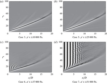
Characteristic diagrams showing the development of the first acoustic wave, vortex ring and shock waves for different inlet conditions. Shown is the pressure perturbation (
 $p^{\prime }$
) history along the jet axis over time.

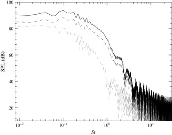
SPL spectrum of the acoustic radiated by the vortex ring in a reference frame moving with the vortex ring: (– ⋅ – ⋅ –) (grey) corresponds to the acoustic radiated at
 $\unicode[STIX]{x1D703}=90^{\circ }$
with respect to the jet axis, (– – – –) corresponds to
 $\unicode[STIX]{x1D703}=135^{\circ }$
and (———–) to
 $\unicode[STIX]{x1D703}=157.5^{\circ }$
.

During the pressure decay, the lower values of
 $p_{r}/p_{\infty }$
cause the shock waves to travel backwards until the lip of the nozzle, figure 17(c). Since the interaction between the shock waves and the vortices of the shear layer play a very important role in the jet noise, the dynamics of the shock waves can be expected to alter the jet noise.
The temporal evolution of the pressure perturbations along the jet axis is shown in figure 17 for four representative cases under study. For
 $t^{\ast }=0$
the whole jet axis is at rest. The oblique line starting at the origin and growing to the right-hand side of the plot is the trace of the vortex ring. After the vortex ring, and close to the lip of the nozzle, the shock waves are created only in cases
 $5$
,
 $6$
and
 $7.a$
. The shock waves are very easy to identify because of the ‘zebra’ pattern in which a combination of a white and a black stripe corresponds to one shock wave, due to the positive and negative pressure relative to the ambient pressure (
 $p-p_{\infty }$
). In these
 $x/D-t^{\ast }$
diagrams, the velocities can be very easily computed by calculating the inverse of the slope of the traces. In figure 17(a), the trace of the first pressure wave can be identified as a oblique line starting from the origin with a flatter slope than the vortex ring, having a reference of the speed of sound at the temperature in the unbounded chamber.
Comparing the slope of the traces of the last shock waves during the decay in figure 17(c) with the slope of the first pressure wave in figure 17(a), we can infer that the last shocks are moving with a Mach number close to unity.
The BBSN is generated by the coherent scattering of the large turbulent structures as they pass through the quasi-periodic shock cells (Tam & Tanna Reference Tam and Tanna1982). Due to the induced velocity of the shock waves during the decay stage, they are expected to have a Doppler effect in the shock associated noise. Moreover, the shock spacing is expected to be reduced, which leads to a shift in frequencies, including the BBSN peak frequency.
4.4.4 Directivity of the noise radiated by the starting jet
The directivity of the different jet noise components is well known in the community for the case of the continuous jet. The TMN is radiated mainly in the downstream direction while the BBSN is radiated mainly in the transverse upstream direction. In case of the existence of screech tones, they are also radiated in the transverse upstream direction.
We present here the different noise sources of the starting jet with their directivity in order to analyse the angular dependence of the SPL spectra for the starting jet.
The front pressure wave is radiated in all directions as a spherical wave, starting at the lip of the nozzle and propagating with the speed of sound. The spectrum of the first pressure wave would be flat, analogous to a Gauss pulse.
The noise produced by the vortex ring is mainly radiated downstream, see figure 18.
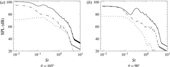
SPL spectra radiated downstream (a) and in the transverse direction (b). Only cases
 $1$
,
 $5$
and
 $7.a$
are represented. Lines as in table 1.

In the starting jet with a trailing jet, TMN is radiated in the downstream direction. BBSN is only radiated when shocks are present in the flow field, that is, in the time interval when the trailing jet is supersonic. In this case the BBSN is radiated, as in the continuous jet, in the transverse upstream direction. The noise radiated by the shock–shear layer–vortex interaction is also radiated in the transverse upstream direction.
We analysed the SPL spectrum in two directions (
 $\unicode[STIX]{x1D703}=165^{\circ }\text{ and }90^{\circ }$
) in order to identify the acoustic footprint of the different physical phenomena. Figure 19(a) shows the streamwise acoustic radiation of the vortex ring in the case
 $1$
, and the turbulent mixing noise in the cases
 $5\text{ and }7.a$
. Except for the low Strouhal numbers, where there is less information, no major differences were found. Figure 19(b) shows the acoustic radiation in the transverse direction (
 $\unicode[STIX]{x1D703}=90^{\circ }$
). Case
 $1$
is qualitatively very different from both cases
 $5\text{ and }7.a$
. From the curve of case
 $7.a$
we identified the frequency range which corresponds to the BBSN, and we identified as well that the curve corresponding to case
 $5$
has the highest frequencies of the BBSN, but not the lowest. The supersonic time interval in case
 $5$
was not long enough to radiate the lowest frequencies of the BBSN.
5 Conclusions
A compressible starting jet can be described by three phases. A compression wave is generated right after the release of pressure, followed by a vortex ring and a compressible trailing jet.
Large Reynolds numbers lead to a pinch-off in a ‘multiple’ way and also dictate the existence of the shear layer–vortex and the shock–shear layer–vortex interaction.
As reported for the incompressible case, there is a limiting value for the dimensionless mass supply in the compressible case that dictates the existence of a trailing jet. Lower values of the dimensionless mass supply lead to lower Mach numbers in the flow field.
The reservoir to chamber pressure ratio plays a crucial role as opposed to the case of the incompressible starting jet: it determines whether the trailing jet and the vortex ring are subsonic or supersonic and it also determines if the front wave remains as a pressure wave or if it is a blast wave.
The shock–shear layer–vortex interaction was reported for the first time. The noise radiated is as loud as the main noise sources of the continuous jet in terms of sound pressure level.
Results can be useful for the characterisation when direct measurements cannot be carried out, for example with volcanic jets.
Acknowledgements
The authors gratefully acknowledge the Gauss Centre for Supercomputing e.V. (www.gauss-centre.eu) for funding this project by providing computing time on the GCS Supercomputer SuperMUC at Leibniz Supercomputing Centre (LRZ, www.lrz.de). This work was supported by the collaborative research centre CRC 1029: ‘Substantial efficiency increase in gas turbines through direct use of coupled unsteady combustion and flow dynamics’.