1 Introduction
Flows over sharp-edged aerofoils are in general separated. Manipulation of this separation in order to achieve beneficial aerodynamic properties is of great practical importance and this topic is therefore subject to a great deal of attention in the scientific and engineering literature. This control of the flow separation is generally aimed at increasing the lift and decreasing the drag experienced by the aerofoil and the control strategies used can broadly be classified as either passive or active. Passive control strategies usually involve some form of geometrical modification to the aerofoil, for example, by deployment of vortex generators such as Gurney flaps (Storms & Jang Reference Storms and Jang1994). Active control strategies, on the other hand, involve the injection or extraction of energy. For instance, synthetic jet actuators are commonly used to perform such flow control over aerofoils (Smith et al. Reference Smith, Amitay, Kibens, Parekh and Glezer1998). Another approach is to use some form of actuation to ‘simulate’ a passive control, for example, by using plasma actuators to imitate Gurney flaps (Feng, Choi & Wang Reference Feng, Choi and Wang2015).
From a physical perspective, the goal of all such devices is to allow shed vortices to convect over the airfoil, past the trapped vortices whose role is to increase the circulation around the aerofoil. For example, in the flow past an inclined flat plate at high Reynolds number, large-scale vortex structures are periodically shed from both the leading and trailing edges of the plate. If a leading-edge vortex could be trapped above the plate, a potentially large gain in lift could be achieved for little cost. It was with this motivation in mind that Witold Kasper designed, and was subsequently granted a patent for, his ‘aircraft wing with vortex generation’ (Kasper Reference Kasper1974). Following test flights investigating the stall characteristics of his BKB-1 glider, Kasper reported lift-to-drag ratios of
 $L/D=17.6$
at the speed of
 $32~\text{km h}^{-1}$
and angle of attack of
 $35^{\circ }$
, considered remarkable at such low speeds (Kruppa Reference Kruppa1977). If such results could be reproduced and verified, they would likely indicate a previously undocumented phenomenon operating on Kasper’s glider. Kasper conjectured that a vortex tube formed above the wing concomitantly increasing the lift and decreasing the drag, a phenomenon coined ‘vortex lift’. He further speculated that this effect could be enhanced by positioning additional ‘flaps’ or auxiliary aerofoils close to the main aerofoil to control the feeding and shedding of vortices in the vicinity of the wing. This configuration, where two additional auxiliary aerofoils are placed off the rear of the main aerofoil, is what is referred to as a ‘Kasper wing’.
Among the first mathematical investigations into the phenomenon of vortex lift was the study carried out by Saffman & Sheffield (Reference Saffman and Sheffield1977), where solutions for steady potential flows consisting of a single point vortex located above a thin flat plate in the presence of a uniform stream were given explicitly. In that study, it was shown that leading- and trailing-edge loci exist for the point-vortex positions that satisfy the steady state condition and that these equilibria are force enhancing, that is, the presence of the point vortex enhances the lift experienced by the aerofoil. Further, a preliminary stability analysis indicated that linearly stable solutions exist only when the vortex is located on the trailing-edge locus not too close to the plate and the angle of attack is greater than approximately
 $8^{\circ }$
. A similar analysis was carried out for the Joukowski aerofoil by Huang & Chow (Reference Huang and Chow1982). Mathematical and computational aspects of control problems involving vortex flows were surveyed by Protas (Reference Protas2008).
Some other studies motivated by vortex trapping mechanisms in the presence of aerofoils include the work of Zannetti & Iollo (Reference Zannetti and Iollo2003) who considered the effect of leading-edge wall suction on stabilization of vortex shedding in the flow over a flat plate at incidence, and the work of Xia & Mohseni (Reference Xia and Mohseni2012) where similar techniques were extended to consider a flapping plate. Investigations of some properties of vortex cells, where an aerofoil contains a cavity specifically designed to trap a vortex, were carried out by Bunyakin, Chernyshenko & Stepanov (Reference Bunyakin, Chernyshenko and Stepanov1998) and more recently by Donelli et al. (Reference Donelli, Iannelli, Chernyshenko, Iollo and Zannetti2009). In the latter study, results from point-vortex, Prandtl–Batchelor flow, and Reynolds-averaged Navier–Stokes models were compared to ascertain the usefulness of inviscid flow models in the design of vortex cells. It was seen that the point-vortex model produced qualitatively similar results to those obtained using the Reynolds-averaged Navier–Stokes system, whilst the Prandtl–Batchelor flow model gave an acceptable representation of these solutions. However, the authors also comment that the vortex is expected to be unstable in the configurations considered.
The trapped vortex is formed from the vorticity in the boundary layer separating from the leading edge of the airfoil which then undergoes the Kelvin–Helmholtz instability, an effect which is not explicitly accounted for by inviscid point vortex and vortex-patch models. However, potential-flow models typically involve free parameters (related to circulations around contours) which make it possible to impose certain additional conditions reflecting viscous effects. In the studies referenced above, the location of the separating streamline is subject to the so-called Kutta condition. Inviscid flows over sharp edges are characterized by unbounded velocity on the boundary in the absence of separation and imposing a Kutta condition at the desired point simultaneously forces the flow to be regular. Gallizio et al. (Reference Gallizio, Iollo, Protas and Zannetti2010) derived precise conditions under which vortex-patch solutions of the two-dimensional Euler equations can be continued with respect to parameters such that nearby solutions also satisfy the Kutta condition. These conditions were illustrated by computing a continuous family of patch solutions connecting the point vortex and the Prandtl–Batchelor solution.
Given that flow configurations with trapped vortices tend to be unstable, the purpose of the present study is to propose and validate practical stabilization strategies. Flow configurations will be based on those of Saffman & Sheffield (Reference Saffman and Sheffield1977) for the single-plate case and those of Nelson & Sakajo (Reference Nelson and Sakajo2014) for the Kasper wing case. We will first provide a control-oriented characterization of the stability of these flow equilibria and will then design a linear–quadratic–Gaussian (LQG) compensator for their stabilization. Flow actuation will be carried out by placing a sink–source singularity at a chosen fixed location on the main plate. Use of the sink–source as an actuation mechanism is intended to mimic the effect of blowing and suction commonly used in control strategies in which viscosity is taken into account. Pressure difference across the plate at a chosen location will be used as the measurement. By analysing the performance of the closed-loop control systems we will demonstrate that in fact the Kasper wing configuration has a positive effect on the robustness of the trapped-vortex equilibria, which is a key finding of this investigation.
The structure of the paper is as follows: in § 2 we state the model equations in the absence of any control actuation, discuss the stability of the different equilibria and identify the equilibrium configurations which will be subject to further analysis. In § 3 we characterize the model from a control-theoretic perspective and in § 4 derive the LQG compensator. Stability properties of the closed-loop system are investigated computationally in § 5, whereas in § 6 the performance of the LQG control is studied in the presence of different perturbations. Further points of discussion and final conclusions are given in §§ 7 and 8.
2 Flow models in the uncontrolled setting
We begin by stating the governing equations for both the single plate and Kasper wing systems and following this survey the stability of some of the equilibria these systems admit. A detailed derivation of these equations is presented in Nelson & Sakajo (Reference Nelson and Sakajo2014), whereas the stability and nonlinear robustness of various configurations is examined in Nelson & Sakajo (Reference Nelson and Sakajo2016). Here, attention is restricted to configurations which will be studied in the controlled setting.
2.1 Governing equations
Let
 ${\mathcal{D}}_{z}$
denote the domain exterior to
 $M+1$
thin plates, where
 $M=0$
corresponds to the single-plate case and
 $M=2$
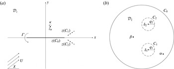
to the Kasper wing case. A schematic of the configurations is shown in figure 1(a). To evaluate the velocity field
 $V(z)=u-\text{i}v$
induced at a point
 $z=x+\text{i}y$
in
 ${\mathcal{D}}_{z}$
, the complex potential of the system is first constructed in a conformally equivalent pre-image circular domain. This circular domain is labelled
 ${\mathcal{D}}_{\unicode[STIX]{x1D701}}$
and consists of the interior of the unit disk with
 $M$
excised non-overlapping smaller disks. The boundary of the unit circle will be labelled
 $C_{0}$
and those of the
 $M$
excised disks
 $C_{k}$
for
 $k=1,\ldots ,M$
. Complex coordinates in the transformed domain will be denoted
 $\unicode[STIX]{x1D701}$
(and thus
 $z=z(\unicode[STIX]{x1D701})$
). Let the centres and radii of the
 $M$
excised disks be respectively
 $\unicode[STIX]{x1D6FF}_{k}\in \mathbb{C}$
and
 $q_{k}\in \mathbb{R}$
for
 $k=1,\ldots ,M$
. An example illustrating such a pre-image domain is shown in figure 1(b). In what follows, overlines will be used to denote complex conjugation and for some complex function
 $f(\unicode[STIX]{x1D701})$
, its conjugate function (Schwarz conjugate) is defined as
 $\bar{f}(\unicode[STIX]{x1D701}):=\overline{f(\bar{\unicode[STIX]{x1D701}})}$
(where ‘
 $:=$
’ means that the expression on the left-hand side is defined by the one on the right-hand side).
(a) Schematic of the flow configuration. The thick dashed lines correspond to the auxiliary plates present in the Kasper wing system (with
 $M=2$
) but not in the single-plate system (with
 $M=0$
). (b) Schematic of a typical pre-image domain.

Let
 $\unicode[STIX]{x1D6FC},\unicode[STIX]{x1D6FD}\in {\mathcal{D}}_{\unicode[STIX]{x1D701}}$
, respectively, denote the location of a point vortex and the point that is mapped to infinity in
 ${\mathcal{D}}_{z}$
, i.e.
 $z(\unicode[STIX]{x1D6FD})=\infty$
. The flow under consideration consists of the following components (for each of which the complex potential at a point
 $\unicode[STIX]{x1D701}$
is stated):
-
(i) a potential flow which tends to a uniform flow inclined at angle
 $\unicode[STIX]{x1D712}_{0}$
as
$|z|\rightarrow \infty$
(2.1)where
$$\begin{eqnarray}W_{U}(\unicode[STIX]{x1D701},\unicode[STIX]{x1D6FD})=Ua\left[\text{e}^{\text{i}\unicode[STIX]{x1D712}_{0}}\frac{\unicode[STIX]{x2202}}{\unicode[STIX]{x2202}\bar{\unicode[STIX]{x1D6FD}}}-\text{e}^{-\text{i}\unicode[STIX]{x1D712}_{0}}\frac{\unicode[STIX]{x2202}}{\unicode[STIX]{x2202}\unicode[STIX]{x1D6FD}}\right]\log \left(\frac{\unicode[STIX]{x1D714}(\unicode[STIX]{x1D701},\unicode[STIX]{x1D6FD})}{|\unicode[STIX]{x1D6FD}|\unicode[STIX]{x1D714}(\unicode[STIX]{x1D701},\bar{\unicode[STIX]{x1D6FD}}^{-1})}\right),\end{eqnarray}$$
$a$
is a scaling constant such that
$|\text{d}W/\text{d}z|\rightarrow U$
as
$|z|\rightarrow \infty$
(see Nelson & Sakajo Reference Nelson and Sakajo2014);
-
(ii) flow due to a single point vortex
(2.2)where
$$\begin{eqnarray}W_{V}(\unicode[STIX]{x1D701};\unicode[STIX]{x1D6FC})=-\frac{\text{i}\unicode[STIX]{x1D705}}{2\unicode[STIX]{x03C0}}\log \left(\frac{\unicode[STIX]{x1D714}(\unicode[STIX]{x1D701},\unicode[STIX]{x1D6FC})}{|\unicode[STIX]{x1D6FC}|\unicode[STIX]{x1D714}(\unicode[STIX]{x1D701},\bar{\unicode[STIX]{x1D6FC}}^{-1})}\right),\end{eqnarray}$$
$\unicode[STIX]{x1D705}$
denotes the circulation of the point vortex;
-
(iii) flow due to a point vortex with circulation
$-\unicode[STIX]{x1D705}$
at the point
$\unicode[STIX]{x1D6FD}$
(to remove the circulation around the disk
$C_{0}$
owing to the point vortex at
$\unicode[STIX]{x1D6FC}$
): (2.3)
$$\begin{eqnarray}W_{\infty }(\unicode[STIX]{x1D701},\unicode[STIX]{x1D6FD})=\frac{\text{i}\unicode[STIX]{x1D705}}{2\unicode[STIX]{x03C0}}\log \left(\frac{\unicode[STIX]{x1D714}(\unicode[STIX]{x1D701},\unicode[STIX]{x1D6FD})}{|\unicode[STIX]{x1D6FD}|\unicode[STIX]{x1D714}(\unicode[STIX]{x1D701},\bar{\unicode[STIX]{x1D6FD}}^{-1})}\right);\end{eqnarray}$$
-
(iv) flows due to prescribed circulations around each of the disks
(2.4)where
$$\begin{eqnarray}W_{\unicode[STIX]{x1D6E4}}(\unicode[STIX]{x1D701},\unicode[STIX]{x1D6FD})=\mathop{\sum }_{k=0}^{M}\frac{\text{i}\unicode[STIX]{x1D6E4}_{k}}{2\unicode[STIX]{x03C0}}\log \left(\frac{\unicode[STIX]{x1D714}(\unicode[STIX]{x1D701},\unicode[STIX]{x1D6FD})}{\unicode[STIX]{x1D714}(\unicode[STIX]{x1D701},\bar{\unicode[STIX]{x1D703}}_{k}(\unicode[STIX]{x1D6FD}^{-1}))}\right),\end{eqnarray}$$
$\unicode[STIX]{x1D6E4}_{k}$
,
$k=0,\ldots ,M$
, is the desired circulation around the disk
$C_{k}$
.


In relations (2.2)–(2.4),
 $\unicode[STIX]{x1D714}(\unicode[STIX]{x1D701},\cdot )$
is a special function known as the Schottky–Klein prime function associated with
 ${\mathcal{D}}_{\unicode[STIX]{x1D701}}$
and
 $\{\unicode[STIX]{x1D703}_{k}\mid k=0,\ldots ,M\}$
are the related Möbius maps. Both of these functions will be described below in § 2.2. The total complex potential in the pre-image domain is then the sum of these components and is thus given by
 $$\begin{eqnarray}W(\unicode[STIX]{x1D701})=W_{\text{V}}(\unicode[STIX]{x1D701};\unicode[STIX]{x1D6FC})+W_{U}(\unicode[STIX]{x1D701},\unicode[STIX]{x1D6FD})+W_{\unicode[STIX]{x1D6E4}}(\unicode[STIX]{x1D701},\unicode[STIX]{x1D6FD})+W_{\infty }(\unicode[STIX]{x1D701},\unicode[STIX]{x1D6FD}).\end{eqnarray}$$
The velocity field in the physical domain is retrieved via (see, e.g., Saffman Reference Saffman1992)
 $$\begin{eqnarray}V(z)=\left\{\begin{array}{@{}ll@{}}(z_{\unicode[STIX]{x1D701}})^{-1}W_{\unicode[STIX]{x1D701}}, & z\neq z(\unicode[STIX]{x1D6FC})\\ (z_{\unicode[STIX]{x1D701}})^{-1}[\widetilde{W}_{\unicode[STIX]{x1D701}}+(\text{i}\unicode[STIX]{x1D705}/4\unicode[STIX]{x03C0})z_{\unicode[STIX]{x1D701}\unicode[STIX]{x1D701}}/z_{\unicode[STIX]{x1D701}}], & z=z(\unicode[STIX]{x1D6FC}),\end{array}\right.\end{eqnarray}$$
where the subscript
 $\unicode[STIX]{x1D701}$
represents the derivative with respect to
 $\unicode[STIX]{x1D701}$
and
 $\widetilde{W}_{\unicode[STIX]{x1D701}}$
is the velocity at the location of the point vortex in the pre-image domain with the self-induction term removed (see, e.g., Saffman Reference Saffman1992). To compute (2.6) it is required to know the form of the conformal mapping
 $z=z(\unicode[STIX]{x1D701})$
from
 ${\mathcal{D}}_{\unicode[STIX]{x1D701}}$
to
 ${\mathcal{D}}_{z}$
. For the domains under consideration, when
 $M=0$
,
 $$\begin{eqnarray}z(\unicode[STIX]{x1D701})=\frac{1}{2}\left(\unicode[STIX]{x1D701}+\frac{1}{\unicode[STIX]{x1D701}}\right)\end{eqnarray}$$
and when
 $M=2$
,
 $$\begin{eqnarray}z(\unicode[STIX]{x1D701})=1+2S\frac{\unicode[STIX]{x1D714}(\unicode[STIX]{x1D701},\unicode[STIX]{x1D6FE})\unicode[STIX]{x1D714}(\unicode[STIX]{x1D701},\bar{\unicode[STIX]{x1D6FE}}^{-1})}{\unicode[STIX]{x1D714}(\unicode[STIX]{x1D701},\unicode[STIX]{x1D6FD})\unicode[STIX]{x1D714}(\unicode[STIX]{x1D701},\bar{\unicode[STIX]{x1D6FD}}^{-1})},\end{eqnarray}$$
where, owing to a degree of freedom in the Riemann mapping theorem,
 $\unicode[STIX]{x1D6FD}$
can be chosen to lie anywhere in
 ${\mathcal{D}}_{\unicode[STIX]{x1D701}}$
, but it will be required to compute the values of
 $S$
and
 $\unicode[STIX]{x1D6FE}$
corresponding to the desired configuration in
 ${\mathcal{D}}_{z}$
.
The map given in (2.7) is the celebrated Joukowski map which maps the unit disk (
 $|\unicode[STIX]{x1D701}|=1$
) to a thin slit located on the real axis (
 $\text{Im}(z)=0$
) between
 $-1\leqslant \text{Re}(z)\leqslant 1$
and the interior of the disk to the region exterior to this slit. Note that, for this map, the point mapped to infinity in
 ${\mathcal{D}}_{z}$
corresponds to
 $\unicode[STIX]{x1D6FD}=0$
. The form of the map appearing in (2.8) is known as a radial slit map (a subset of the more general group of conformal slit maps). Such maps have a wide range of applications in applied mathematics (Crowdy Reference Crowdy2012). Here, the map (2.8) will again map the unit disk to a thin slit located on the real axis between
 $-1\leqslant z\leqslant 1$
. Additionally, the two excised disks will be mapped to sections of ‘radial rays’ emanating from the point
 $z=1$
. The region interior to the unit disk and exterior to the two excised disks will be mapped to the region exterior to the three radial thin plates. It should be noted that the appearance of the Schottky–Klein prime function in (2.8) is a consequence of the type of conformal map required here and is not directly related to its appearance in (2.2)–(2.4). Further details regarding the relation between these maps and the configurations desired will be given shortly.
With the velocity field throughout
 ${\mathcal{D}}_{z}$
determined, the instantaneous position of the free point vortex, which we will denote
 $\boldsymbol{X}(t):=[x~y]^{\text{T}}=[\text{Re}(z)~\text{Im}(z)]^{\text{T}}$
, is governed by the nonlinear dynamical system
 $$\begin{eqnarray}\frac{\text{d}}{\text{d}t}\boldsymbol{X}=\boldsymbol{F}(\boldsymbol{X})=\left[\begin{array}{@{}l@{}}\phantom{-}\text{Re}[V(z)]\\ -\text{Im}[V(z)]\end{array}\right].\end{eqnarray}$$
First, stationary solutions are sought such that, in addition to the point vortex being in equilibrium, the Kutta conditions prescribing the flow separation at the trailing edge of each plate are satisfied. This choice is motivated by the original study of Saffman & Sheffield (Reference Saffman and Sheffield1977) on the single-plate configuration and more discussion regarding this choice can be found in Nelson & Sakajo (Reference Nelson and Sakajo2014, Reference Nelson and Sakajo2016). Imposing Kutta conditions at each trailing edge means that altogether
 $M+3$
equations must be satisfied, i.e. the Kutta conditions at
 $(M+1)$
plates and two conditions for the equilibrium coordinates
 $\text{Re}(z_{\unicode[STIX]{x1D6FC}})$
and
 $\text{Im}(z_{\unicode[STIX]{x1D6FC}})$
of the point vortex. The unknowns in the problem thus are
 $\{\text{Re}(z_{\unicode[STIX]{x1D6FC}}),\text{Im}(z_{\unicode[STIX]{x1D6FC}}),\unicode[STIX]{x1D705},\unicode[STIX]{x1D6E4}_{0},\ldots ,\unicode[STIX]{x1D6E4}_{M}\}$
giving
 $M+4$
real numbers. Solutions are therefore expected to trace out one-parameter continuous loci. Labelling the position of the trailing edge of each plate
 $z_{k}$
for
 $k=0,\ldots ,M$
, stationary solutions with a point vortex at
 $z_{\unicode[STIX]{x1D6FC}}$
are characterized by
 $$\begin{eqnarray}\displaystyle & \displaystyle \text{Re}[V(z_{\unicode[STIX]{x1D6FC}};\unicode[STIX]{x1D712}_{0},\unicode[STIX]{x1D705},\unicode[STIX]{x1D6E4}_{0},\ldots ,\unicode[STIX]{x1D6E4}_{M})]=0, & \displaystyle\end{eqnarray}$$
 $$\begin{eqnarray}\displaystyle & \displaystyle \text{Im}[V(z_{\unicode[STIX]{x1D6FC}};\unicode[STIX]{x1D712}_{0},\unicode[STIX]{x1D705},\unicode[STIX]{x1D6E4}_{0},\ldots ,\unicode[STIX]{x1D6E4}_{M})]=0, & \displaystyle\end{eqnarray}$$
 $$\begin{eqnarray}\displaystyle & \displaystyle |V(z_{k};\unicode[STIX]{x1D712}_{0},\unicode[STIX]{x1D705},\unicode[STIX]{x1D6E4}_{0},\ldots ,\unicode[STIX]{x1D6E4}_{M})|=0,\quad k=0,\ldots ,M, & \displaystyle\end{eqnarray}$$
 $\unicode[STIX]{x1D712}_{0}$
can be chosen freely and the unknowns
 $z_{\unicode[STIX]{x1D6FC}},\unicode[STIX]{x1D705},\unicode[STIX]{x1D6E4}_{0},\ldots ,\unicode[STIX]{x1D6E4}_{M}$
are solved for. For the single-plate case (
 $M=0$
), equations (2.10) can be solved exactly. However, closed-form solutions are not possible for the Kasper wing system (
 $M=2$
) and a numerical approach is required. As in Nelson & Sakajo (Reference Nelson and Sakajo2014, Reference Nelson and Sakajo2016), a Brownian ratchets scheme is used to solve equations (2.10) to within a prescribed numerical tolerance. Further details regarding such Brownian ratchets schemes can be found in Newton & Chamoun (Reference Newton and Chamoun2007).
2.2 The Schottky–Klein prime function
In this section the aforementioned Schottky–Klein prime function and the associated Möbius maps are briefly introduced. For further details regarding this function and its properties we refer the reader to, e.g., Crowdy & Marshall (Reference Crowdy and Marshall2005). One manner in which this special function can be evaluated is via a classic product formula (Baker Reference Baker1897). Within
 ${\mathcal{D}}_{\unicode[STIX]{x1D701}}$
, for each of the
 $M$
excised circles
 $C_{k}$
,
 $k=1,\ldots ,M$
, we construct the Möbius map
 $$\begin{eqnarray}\unicode[STIX]{x1D703}_{k}(\unicode[STIX]{x1D701})=\unicode[STIX]{x1D6FF}_{k}+\frac{q_{k}^{2}\unicode[STIX]{x1D701}}{1-\bar{\unicode[STIX]{x1D6FF}}_{k}\unicode[STIX]{x1D701}}.\end{eqnarray}$$
The Schottky–Klein prime function is then given by
 $$\begin{eqnarray}\unicode[STIX]{x1D714}(\unicode[STIX]{x1D701},\unicode[STIX]{x1D6FE})=(\unicode[STIX]{x1D701}-\unicode[STIX]{x1D6FE})\mathop{\prod }_{\unicode[STIX]{x1D717}\in \unicode[STIX]{x1D6E9}^{\prime \prime }}\frac{[\unicode[STIX]{x1D717}(\unicode[STIX]{x1D701})-\unicode[STIX]{x1D6FE}][\unicode[STIX]{x1D717}(\unicode[STIX]{x1D6FE})-\unicode[STIX]{x1D701}]}{[\unicode[STIX]{x1D717}(\unicode[STIX]{x1D701})-\unicode[STIX]{x1D701}][\unicode[STIX]{x1D717}(\unicode[STIX]{x1D6FE})-\unicode[STIX]{x1D6FE}]},\end{eqnarray}$$
where the product is taken over all mappings
 $\unicode[STIX]{x1D717}$
belonging to a special subset
 $\unicode[STIX]{x1D6E9}^{\prime \prime }$
of the full Schottky group
 $\unicode[STIX]{x1D6E9}$
. (The full, or classical, Schottky group
 $\unicode[STIX]{x1D6E9}$
is defined to be the infinite free group of mappings generated by compositions of the
 $M$
basic Möbius maps
 $\{\unicode[STIX]{x1D703}_{k}\mid k=1,\ldots ,M\}$
and their inverses
 $\{\unicode[STIX]{x1D703}_{k}^{-1}\mid k=1,\ldots ,M\}$
and including the identity map.) This subset contains all mappings, excluding the identity and all inverse mappings, thus, for example, if the map
 $\unicode[STIX]{x1D703}_{1}\unicode[STIX]{x1D703}_{2}^{-1}$
is included in the set,
 $\unicode[STIX]{x1D703}_{2}\unicode[STIX]{x1D703}_{1}^{-1}$
must be excluded. Two important properties of the Schottky–Klein prime function are:
-
(i)
$\unicode[STIX]{x1D714}(\unicode[STIX]{x1D701},\unicode[STIX]{x1D6FE})$
has a simple zero at
$\unicode[STIX]{x1D701}=\unicode[STIX]{x1D6FE}$
; -
(ii)
$\unicode[STIX]{x1D714}(\cdot ,\cdot )$
is such that the complex potential has constant imaginary part on all circles
$C_{k}$
,
$k=0,1,\ldots ,M$
.


Formula (2.12) is useful for concisely stating
 $\unicode[STIX]{x1D714}(\cdot ,\cdot )$
and can be applied in some practical situations. In general, however, expression (2.12) fails to converge or requires an impractically long time to compute (for example, when two circles are close together or when the connectivity is high). A more robust method is to compute
 $\unicode[STIX]{x1D714}(\cdot ,\cdot )$
via a Fourier–Laurent expansion, details of which are presented in Crowdy & Marshall (Reference Crowdy and Marshall2007). Briefly, the algorithm works by introducing the function
 $X(\cdot ,\cdot )$
defined as
 $$\begin{eqnarray}X(\unicode[STIX]{x1D701},\unicode[STIX]{x1D6FE})=(\unicode[STIX]{x1D701}-\unicode[STIX]{x1D6FE})^{2}\hat{X}(\unicode[STIX]{x1D701},\unicode[STIX]{x1D6FE}),\end{eqnarray}$$
in which
 $$\begin{eqnarray}\hat{X}(\unicode[STIX]{x1D701},\unicode[STIX]{x1D6FE})=A\left[1+\mathop{\sum }_{k=1}^{M}\mathop{\sum }_{m=1}^{\infty }\left(\frac{c_{m}^{(k)}q_{k}^{m}}{(\unicode[STIX]{x1D701}-\unicode[STIX]{x1D6FF}_{k})^{m}}+\frac{d_{m}^{(k)}Q_{k}^{m}}{(\unicode[STIX]{x1D701}-\unicode[STIX]{x1D6FF}_{k}^{\prime })^{m}}\right)\right],\end{eqnarray}$$
where
 $\unicode[STIX]{x1D6FF}_{k}^{\prime }$
is the centre of the circle
 $C_{k}^{\prime }$
obtained from reflecting
 $C_{k}$
about
 $|\unicode[STIX]{x1D701}|=1$
,
 $Q_{k}$
is related to the radius of
 $C_{k}^{\prime }$
, the constants
 $\{c_{m}^{(k)},d_{m}^{(k)}\mid k=1,\ldots ,M,m=1,2,\ldots \}$
are determined numerically (for some truncated
 $m$
) and
 $A$
is a normalization coefficient chosen such that
 $$\begin{eqnarray}\lim _{\unicode[STIX]{x1D701}\rightarrow \unicode[STIX]{x1D6FE}}\frac{X(\unicode[STIX]{x1D701},\unicode[STIX]{x1D6FE})}{(\unicode[STIX]{x1D701}-\unicode[STIX]{x1D6FE})^{2}}=1.\end{eqnarray}$$
The Schottky–Klein prime function is then retrieved via
 $$\begin{eqnarray}X^{2}(\unicode[STIX]{x1D701},\unicode[STIX]{x1D6FE})=\unicode[STIX]{x1D714}(\unicode[STIX]{x1D701},\unicode[STIX]{x1D6FE}),\end{eqnarray}$$
where the branch of the square root is taken such that
 $\unicode[STIX]{x1D714}(\unicode[STIX]{x1D701},\unicode[STIX]{x1D6FE})$
behaves like
 $(\unicode[STIX]{x1D701}-\unicode[STIX]{x1D6FE})$
as
 $\unicode[STIX]{x1D701}\rightarrow \unicode[STIX]{x1D6FE}$
.
2.3 Linear stability analysis of point-vortex equilibria
Linear stability analysis of the single plate and Kasper wing systems is carried out by adding a small perturbation
 $z^{\prime }=x^{\prime }+\text{i}y^{\prime }$
to the point-vortex equilibrium
 $z_{\unicode[STIX]{x1D6FC}}$
and performing linearization. The evolution of this perturbation is governed by the system
 $$\begin{eqnarray}\frac{\text{d}}{\text{d}t}\boldsymbol{X}^{\prime }=\unicode[STIX]{x1D63C}\boldsymbol{X}^{\prime },\end{eqnarray}$$
where
 $\boldsymbol{X}^{\prime }(t)=[x^{\prime }(t)~y^{\prime }(t)]^{\text{T}}$
and
 $\unicode[STIX]{x1D63C}$
is given by (see Nelson & Sakajo Reference Nelson and Sakajo2016)
 $$\begin{eqnarray}\unicode[STIX]{x1D63C}=\left[\begin{array}{@{}cc@{}}a & \phantom{-}b\\ c & -a\end{array}\right],\end{eqnarray}$$
with
 $$\begin{eqnarray}\displaystyle & \displaystyle a=\text{Re}\left[\left.\frac{\unicode[STIX]{x2202}V}{\unicode[STIX]{x2202}z}\right|_{\bar{z}_{\unicode[STIX]{x1D6FC}}}\right], & \displaystyle\end{eqnarray}$$
 $$\begin{eqnarray}\displaystyle & \displaystyle b=-\text{Im}\left[\left.\frac{\unicode[STIX]{x2202}V}{\unicode[STIX]{x2202}z}\right|_{\bar{z}_{\unicode[STIX]{x1D6FC}}}\right]+\text{Im}\left[\left.\frac{\unicode[STIX]{x2202}V}{\unicode[STIX]{x2202}\bar{z}}\right|_{z_{\unicode[STIX]{x1D6FC}}}\right], & \displaystyle\end{eqnarray}$$
 $$\begin{eqnarray}\displaystyle & \displaystyle c=-\text{Im}\left[\left.\frac{\unicode[STIX]{x2202}V}{\unicode[STIX]{x2202}z}\right|_{\bar{z}_{\unicode[STIX]{x1D6FC}}}\right]-\text{Im}\left[\left.\frac{\unicode[STIX]{x2202}V}{\unicode[STIX]{x2202}\bar{z}}\right|_{z_{\unicode[STIX]{x1D6FC}}}\right]. & \displaystyle\end{eqnarray}$$
 $\unicode[STIX]{x1D63C}$
reveals that the system is:
-
(i) unstable when
$a^{2}+bc>0$
(corresponding to purely real eigenvalues); -
(ii) neutrally stable when
$a^{2}+bc<0$
(corresponding to purely imaginary eigenvalues).


We emphasize that when the linearization has purely imaginary eigenvalues and there are no eigenvalues with positive real parts, as is the case here, then such linearization is inconclusive as regards the stability properties of the equilibrium and one must account for the effect of nonlinearity through suitable invariant manifold reductions (Protas Reference Protas2007). We also note that, since system (2.9) is Hamiltonian, the two eigenvalues may be either purely real and of opposite signs or form a conjugate imaginary pair (Newton Reference Newton2001). It should also be noted that when the system is perturbed away from the equilibrium, the Kutta conditions (2.10c ) are no longer satisfied. For these conditions to be satisfied throughout any time-dependent evolution, a method for shedding vorticity from the rear tip of each plate is required. This topic will be revisited in § 6.
2.4 Configurations and analysis
We now introduce the configurations which will be subject to further study and analyse their properties in the uncontrolled setting. In all configurations, the main plate (which
 $C_{0}$
is mapped to) will lie in the region defined by
 $-1\leqslant x\leqslant 1$
and
 $y=0$
and, when
 $M=2$
, the centres of the auxiliary plates (which
 $C_{1}$
and
 $C_{2}$
are mapped to) will lie at
 $z=1+0.4\text{e}^{\pm \text{i}\unicode[STIX]{x1D719}}$
. Three values of the angle
 $\unicode[STIX]{x1D719}$
will be used, these being
 $\unicode[STIX]{x03C0}/12$
,
 $\unicode[STIX]{x03C0}/6$
and
 $5\unicode[STIX]{x03C0}/12$
, and the length of the auxiliary plates will be set to
 $0.1$
. This means that
 $C_{1}$
and
 $C_{2}$
are mapped to straight segments with endpoints, respectively, at
 $z=1+(0.4\pm 0.05)\text{e}^{\text{i}\unicode[STIX]{x1D719}}$
and
 $z=1+(0.4\pm 0.05)\text{e}^{-\text{i}\unicode[STIX]{x1D719}}$
. The angle of attack of the oncoming flow is set to
 $\unicode[STIX]{x1D712}_{0}=0.1$
.
Owing to the configurations chosen in
 ${\mathcal{D}}_{z}$
, when
 $M=2$
,
 $\unicode[STIX]{x1D6FE}$
must be set unity. The constant
 $\unicode[STIX]{x1D6FD}$
can be chosen freely and will be set to
 $-0.4$
in all results that follow. In the construction of
 ${\mathcal{D}}_{\unicode[STIX]{x1D701}}$
and the conformal map, the remaining unknowns are
 $S,\unicode[STIX]{x1D6FF}_{1},q_{1},\unicode[STIX]{x1D706}_{1}$
and
 $\unicode[STIX]{x1D706}_{2}$
, where
 $\unicode[STIX]{x1D706}_{1}$
and
 $\unicode[STIX]{x1D706}_{2}$
are the angles (with respect to
 $\unicode[STIX]{x1D6FF}_{1}$
) of the points on
 $C_{1}$
that map to the auxiliary plate edges in
 ${\mathcal{D}}_{z}$
, which leaves six real unknowns. We note that due to the symmetry of the configurations considered here,
 $\unicode[STIX]{x1D6FF}_{2}=\overline{\unicode[STIX]{x1D6FF}_{1}}$
and
 $q_{2}=q_{1}$
(see Nelson & Sakajo (Reference Nelson and Sakajo2016) for details regarding non-symmetric Kasper wing configurations). The six unknowns can be found from the six real-valued equations obtained from
 $$\begin{eqnarray}\displaystyle & \displaystyle z(-1)=-1, & \displaystyle\end{eqnarray}$$
 $$\begin{eqnarray}\displaystyle & \displaystyle |z(\unicode[STIX]{x1D6FF}_{1}+q_{1}\text{e}^{\text{i}\unicode[STIX]{x1D706}_{1}})-1|=0.35, & \displaystyle\end{eqnarray}$$
 $$\begin{eqnarray}\displaystyle & \displaystyle |z(\unicode[STIX]{x1D6FF}_{1}+q_{1}\text{e}^{\text{i}\unicode[STIX]{x1D706}_{2}})-1|=0.45, & \displaystyle\end{eqnarray}$$
 $$\begin{eqnarray}\displaystyle & \displaystyle \text{Arg}[z(\unicode[STIX]{x1D6FF}_{1}+q_{1}\text{e}^{\text{i}\unicode[STIX]{x1D706}_{2}})]=\unicode[STIX]{x1D719}, & \displaystyle\end{eqnarray}$$
 $$\begin{eqnarray}\displaystyle & \displaystyle \left|\frac{\text{d}z}{\text{d}\unicode[STIX]{x1D701}}(\unicode[STIX]{x1D6FF}_{1}+q_{1}\text{e}^{\text{i}\unicode[STIX]{x1D706}_{1}})\right|=0, & \displaystyle\end{eqnarray}$$
 $$\begin{eqnarray}\displaystyle & \displaystyle \left|\frac{\text{d}z}{\text{d}\unicode[STIX]{x1D701}}(\unicode[STIX]{x1D6FF}_{1}+q_{1}\text{e}^{\text{i}\unicode[STIX]{x1D706}_{2}})\right|=0. & \displaystyle\end{eqnarray}$$
 $\unicode[STIX]{x1D719}$
are given in table 1. The scaling constant
 $a$
(appearing in (2.1)) must be set to
 $$\begin{eqnarray}a=1/2\end{eqnarray}$$
when
 $M=0$
, and
 $$\begin{eqnarray}a=2S\frac{\unicode[STIX]{x1D714}(\unicode[STIX]{x1D6FD},\unicode[STIX]{x1D6FE})\unicode[STIX]{x1D714}(\unicode[STIX]{x1D6FD},\bar{\unicode[STIX]{x1D6FE}}^{-1})}{\unicode[STIX]{x1D714}(\unicode[STIX]{x1D6FD},\bar{\unicode[STIX]{x1D6FD}}^{-1})},\end{eqnarray}$$
when
 $M=2$
. Loci of solutions will be parametrized in terms of their vertical coordinate in the physical domain. Thus, moving along any given locus will correspond to an increasing
 $\text{Im}(z_{\unicode[STIX]{x1D6FC}})$
. Additionally, since they are more relevant from the physical point of view, only loci stemming from the rear tip of the main plate will be considered (see Nelson & Sakajo Reference Nelson and Sakajo2014).
Solutions of equations (2.20) for three different values of
 $\unicode[STIX]{x1D719}$
.

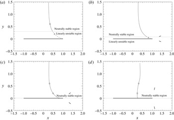
Rear tip equilibria and their linear stability for (a)
 $M=0$
(b)
 $M=2$
,
 $\unicode[STIX]{x1D719}=\unicode[STIX]{x03C0}/12$
, (c)
 $M=2$
,
 $\unicode[STIX]{x1D719}=\unicode[STIX]{x03C0}/6$
and (d)
 $M=2$
,
 $\unicode[STIX]{x1D719}=5\unicode[STIX]{x03C0}/12$
. Thick solid lines represent plates, whereas thin solid and dashed curves represent, respectively, the neutrally stable and unstable parts of the loci. The dotted horizontal lines separate the sections of the equilibrium loci characterized by linear instability and neutral stability. Square and triangle symbols represent, respectively, the locations of neutrally stable and unstable equilibria that will be subject to further analysis (information regarding these equilibria is summarized below in table 2).

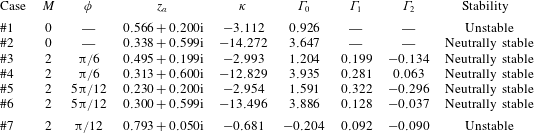
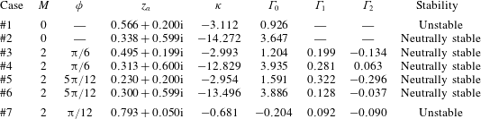
Figure 2(a)–(d) shows the equilibrium loci emanating from the rear tip of the main plate of the configurations just introduced and we also identify parts of the loci characterized by different stability properties. For the configuration with
 $M=0$
, it is seen that a linearly unstable region exists close to the plate (for
 $0<\text{Im}(z_{\unicode[STIX]{x1D6FC}})\lessapprox 0.3$
). Small perturbations to equilibria with
 $z_{\unicode[STIX]{x1D6FC}}$
further away from the main plate exhibit neutral stability. When
 $M=2$
and
 $\unicode[STIX]{x1D719}=\unicode[STIX]{x03C0}/12$
, the shape of the locus and stability properties are relatively similar to the case with
 $M=0$
, but the unstable region has shrunk substantially so that now only equilibria lying in the region with
 $\text{Im}(z_{\unicode[STIX]{x1D6FC}})\lessapprox 0.075$
exhibit linear instability. Again, above this unstable region small perturbations exhibit neutral stability. For the configuration with
 $M=2$
and
 $\unicode[STIX]{x1D719}=\unicode[STIX]{x03C0}/6$
, the unstable region shrinks even further so that linear instability is only witnessed when
 $\text{Im}(z_{\unicode[STIX]{x1D6FC}})\lessapprox 0.003$
. However, when
 $M=2$
and
 $\unicode[STIX]{x1D719}=5\unicode[STIX]{x03C0}/12$
, the shape of the locus and the corresponding stability properties of equilibria change quite dramatically. Equilibria stemming from the rear tip of the main plate remain extremely close to the plate prior to a sharp rise away from it when
 $\text{Re}(z_{\unicode[STIX]{x1D6FC}})$
is roughly
 $0.2$
(given the finite graphical resolution, this latter region cannot be discerned in figure 2
d). The neutrally stable region now also extends down to the plate and unstable equilibria are present only in a small neighbourhood of the rear tip.
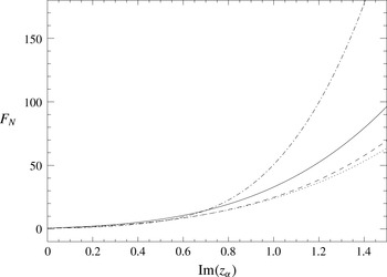
For each configuration, the lift force experienced by the main plate for increasing
 $\text{Im}(z_{\unicode[STIX]{x1D6FC}})$
is shown in figure 3. These forces are computed using the Blasius formula (Crowdy Reference Crowdy2006)
 $$\begin{eqnarray}F_{x}-\text{i}F_{y}=\frac{\text{i}}{2}\oint _{C_{0}}\left(\frac{\text{d}W}{\text{d}z}\right)^{2}\text{d}z,\end{eqnarray}$$
where
 $F_{x}$
and
 $F_{y}$
are the force components acting in the directions
 $x$
and
 $y$
with integration carried out numerically using a trapezoidal rule. The lift,
 $F_{N}$
, is then retrieved through taking the component of (2.23) in the direction normal to the oncoming flow. For small values of
 $\text{Im}(z_{\unicode[STIX]{x1D6FC}})$
the lift experienced by the main plate is similar for all flow configurations. As
 $\text{Im}(z_{\unicode[STIX]{x1D6FC}})$
increases, the lift in the configuration with
 $M=2$
and
 $\unicode[STIX]{x1D719}=\unicode[STIX]{x03C0}/12$
grows slowest, whereas for vortex equilibria furthest away from the plate the configuration with
 $M=2$
and
 $\unicode[STIX]{x1D719}=5\unicode[STIX]{x03C0}/12$
experiences the highest lifts. In regard to the data shown in figure 3, we can conclude that in all cases with auxiliary plates the lift
 $F_{N}$
increases continuously with the inclination angle
 $\unicode[STIX]{x1D719}$
from values lower than in the single-plate configuration (
 $M=0$
) to higher values. In particular, when the inclination angle is close to
 $\unicode[STIX]{x1D719}=3\unicode[STIX]{x03C0}/10$
, the lift is comparable to its value in the single-plate configuration. Although the configurations with small inclination angles
 $\unicode[STIX]{x1D719}$
have smaller lift than the single-plate configuration, they can still be useful since, as shown in figure 2, they are characterized by more favourable stability properties. In addition, differences in lift become more evident only for vortex equilibria located further away from the main plate, i.e. with larger
 $\text{Im}(z_{\unicode[STIX]{x1D6FC}})$
, which are less relevant from the application point of view.
Lift
 $F_{N}$
against
 $\text{Im}(z_{\unicode[STIX]{x1D6FC}})$
. The solid curve represents the single-plate configuration (with
 $M=0$
), the dotted curve the configuration with
 $M=2$
and
 $\unicode[STIX]{x1D719}=\unicode[STIX]{x03C0}/12$
, the dashed curve the configuration with
 $M=2$
and
 $\unicode[STIX]{x1D719}=\unicode[STIX]{x03C0}/6$
and the dot-dash curve the configuration with
 $M=2$
and
 $\unicode[STIX]{x1D719}=5\unicode[STIX]{x03C0}/12$
.

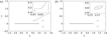
Trajectories (represented by the solid curves) of the solutions of system (2.9) in (a) case #3 and (b) case #4 (see table 2) in which the equilibria
 $z_{\unicode[STIX]{x1D6FC}}$
are perturbed to
 $z_{\unicode[STIX]{x1D6FC}}+\unicode[STIX]{x1D6FF}$
, where
 $\unicode[STIX]{x1D6FF}=0.005\text{i}$
, corresponding to the time interval
 $0\leqslant t\leqslant 50$
. The dotted rectangles represent the regions magnified in the insets. In the magnified regions the solid circle marks the unperturbed equilibrium.

Finally in this section, uncontrolled point-vortex trajectories are presented for configurations with
 $M=2$
and
 $\unicode[STIX]{x1D719}=\unicode[STIX]{x03C0}/6$
. Evolutions are computed through numerical integration of system (2.9) using Euler’s explicit method with a time step of
 $\text{d}t=0.001$
(the choice of this method is motivated by its straightforward extension to the stochastic case considered in § 6.1). Figure 4(a) and (b) show the trajectories of the vortex when it is perturbed by
 $0.005\text{i}$
away from the equilibria, respectively, at
 $\text{Im}(z_{\unicode[STIX]{x1D6FC}})\approx 0.2$
and
 $\text{Im}(z_{\unicode[STIX]{x1D6FC}})\approx 0.6$
. Responses to these perturbations show good agreement with the linear theory for
 $\text{Im}(z_{\unicode[STIX]{x1D6FC}})\approx 0.6$
; that is, the vortex follows a closed orbit over a long period of time. However, when
 $\text{Im}(z_{\unicode[STIX]{x1D6FC}})\approx 0.2$
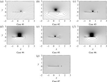
, the vortex quickly escapes showing that nonlinear effects become important even for very small perturbations. Again, it should be noted that during these evolutions the Kutta conditions are not enforced. We emphasize that, from the practical point of view, neutrally stable equilibria are not desirable, because neutral stability in the linearized setting does not imply the stability of the nonlinear system, an effect already observed in figure 4(a). In addition, vortices moving along closed trajectories circumscribing the equilibrium give rise to fluctuating loads on the airfoils which degrade their performance. To close this section, in table 2 we collect the information about the different cases which were discussed here and which will be further studied in the controlled setting below. These cases have been selected to be representative of the different behaviours in the controlled setting (cf. §§ 5 and 6). Note that due to the proximity of the vortex to the main plate in case #7, this case it is not necessarily as physically important as the others considered. It is however included in this study for completeness so that a Kasper wing configuration demonstrating linear instability is represented as well. It is also noted that this case will not be analysed in as much detail as the others considered. To complete the physical picture, the streamline patterns corresponding to the seven equilibrium configurations from table 2 are presented in figure 5. We see that the cases corresponding to equilibrium locations further away from the main plate feature larger recirculation regions.
Summary information about the different flow cases which will be analysed in the subsequent sections.
(a–g) The streamline patterns
 $\unicode[STIX]{x1D713}=\text{Im}[W]$
corresponding to the vortex equilibria from table 2.

3 Control-oriented characterization of the flow model
In the present study the intensity of a point sink–source located on the upper boundary of the main plate is used as the control variable. Other choices of flow actuation are also possible and, for example, circular cylinder rotation was used in the work of Protas (Reference Protas2004). The effect of the sink–source is represented by the addition of a new term to system (2.9) which is now written as
 $$\begin{eqnarray}\frac{\text{d}}{\text{d}t}\boldsymbol{X}=\boldsymbol{F}(\boldsymbol{X})+m\boldsymbol{b}(\boldsymbol{X}),\end{eqnarray}$$
where
 $m$
is the sink–source strength and
 $$\begin{eqnarray}\boldsymbol{b}(\boldsymbol{X})=\left[\begin{array}{@{}l@{}}\text{Re}[\text{d}W_{S}(z)/\text{d}z]\\ -\text{Im}[\text{d}W_{S}(z)/\text{d}z]\!\!\end{array}\right],\end{eqnarray}$$
in which
 $W_{S}(z)$
represents the potential induced at the point
 $z$
by the unit sink–source. First, we note that since the actuator is chosen to lie on upper side of the main plate, its location in the pre-image domain, labelled
 $\unicode[STIX]{x1D701}_{a}$
, will be restricted to
 $\unicode[STIX]{x1D701}_{a}=\exp (-\text{i}\unicode[STIX]{x1D70E})$
for
 $0<\unicode[STIX]{x1D70E}<\unicode[STIX]{x03C0}$
. Then, in the physical domain,
 $z_{a}=z(\unicode[STIX]{x1D701}_{a})$
is such that
 $-1<\text{Re}(z_{a})<1$
and
 $\text{Im}(z_{a})=0$
. Hereafter
 $x_{a}:=\text{Re}(z_{a})$
will denote the location of the sink–source actuator. The complex potential owing to the point sink–source singularity in the pre-image domain is given by
 $$\begin{eqnarray}W_{s}(\unicode[STIX]{x1D701})=\frac{1}{2\unicode[STIX]{x03C0}}\log \left[\frac{\unicode[STIX]{x1D714}(\unicode[STIX]{x1D701},\unicode[STIX]{x1D701}_{a})\unicode[STIX]{x1D714}(\unicode[STIX]{x1D701},\bar{\unicode[STIX]{x1D701}}_{a}^{-1})}{\unicode[STIX]{x1D714}(\unicode[STIX]{x1D701},\unicode[STIX]{x1D6FD})\unicode[STIX]{x1D714}(\unicode[STIX]{x1D701},\bar{\unicode[STIX]{x1D6FD}}^{-1})}\right].\end{eqnarray}$$
Introducing
 $$\begin{eqnarray}W_{S}(z(\unicode[STIX]{x1D701}))=W_{s}(\unicode[STIX]{x1D701}),\end{eqnarray}$$
the derivatives appearing in (3.2) can now be evaluated. Re-deriving the linearized system with the additional term representing the flow actuation, cf. (3.2), gives
 $$\begin{eqnarray}\frac{\text{d}}{\text{d}t}\boldsymbol{X}^{\prime }=\unicode[STIX]{x1D63C}\boldsymbol{X}^{\prime }+m\unicode[STIX]{x1D63D},\end{eqnarray}$$
where
 $\unicode[STIX]{x1D63D}$
is a
 $2\times 1$
matrix obtained from evaluating (3.2) at the equilibrium
 $z_{\unicode[STIX]{x1D6FC}}$
.
In order to formulate a meaningful control problem, it is required to identify a physical objective that the control algorithm will seek to achieve. This objective will be expressed in terms of system outputs, i.e. certain measurable quantities that characterize the system evolution and the system input, i.e. the control strength
 $m$
. Taking some equilibrium configuration as the ‘base’ state, we choose elimination of perturbations to the pressure difference between two points on the main plate boundary resulting from perturbations to this base state as the control objective. The two measurement points labelled
 $z_{+}$
and
 $z_{-}$
are chosen to have the same real coordinate and lie on the upper and lower sides of the plate, so that in
 ${\mathcal{D}}_{z}$
,
 $z_{+}=z_{-}\in [-1,1]\subset \mathbb{R}$
. Introducing the inverse map from the physical to pre-image domain as
 $$\begin{eqnarray}\unicode[STIX]{x1D701}=\unicode[STIX]{x1D701}(z),\end{eqnarray}$$
we have the relation
 $\unicode[STIX]{x1D701}(z_{-})=\overline{\unicode[STIX]{x1D701}(z_{+})}$
, where both points will lie on the unit circle
 $C_{0}$
. In a potential flow the pressure
 $p_{m}$
at a given boundary point can be calculated from the Bernoulli equation as
 $p_{m}=p_{0}+(|V_{0}|^{2}-|V_{m}|^{2})/2$
, where
 $p_{0}$
and
 $V_{0}$
are the pressure and complex velocity at some arbitrary point in the flow domain, and
 $V_{m}$
is the complex velocity at the boundary point. Thus, the pressure difference across the main plate can be calculated as
 $\unicode[STIX]{x0394}p=(|V(z_{+})|^{2}-|V(z_{-})|^{2})/2$
. Choosing this quantity as an output of system (3.1) gives the following output equation
 $$\begin{eqnarray}h(z_{\unicode[STIX]{x1D6FC}}):={\textstyle \frac{1}{2}}\left[|V(z_{+})+mD_{+}|^{2}-|V(z_{-})+mD_{-}|^{2}\right],\end{eqnarray}$$
where
 $V(z_{+/-})$
is obtained from evaluating (2.6) at
 $z_{+/-}$
and
 $$\begin{eqnarray}D_{+}=\left.\frac{\text{d}W_{S}}{\text{d}z}\right|_{z_{+}},\quad D_{-}=\left.\frac{\text{d}W_{S}}{\text{d}z}\right|_{z_{-}}.\end{eqnarray}$$
Linearizing for small
 $m$
then gives
 $$\begin{eqnarray}h(z_{\unicode[STIX]{x1D6FC}})\cong {\textstyle \frac{1}{2}}\left[|V(z_{+})|^{2}-|V(z_{-})|^{2}\right]+mD,\end{eqnarray}$$
where
 $$\begin{eqnarray}D={\textstyle \frac{1}{2}}\left[\overline{V(z_{+})}D_{+}+V(z_{+})\overline{D_{+}}-\overline{V(z_{-})}D_{-}-V(z_{-})\overline{D_{-}}\right],\end{eqnarray}$$
is a scalar representing the direct effect of the control on the measurement (i.e. the control-to-measurement map) in the linearized regime. This particular choice of the observation operator
 $h$
is motivated by practical considerations, as measurements of pressure differences across a wing are relatively easy to implement in a laboratory experiment (i.e. either by direct measurement using instrumentation, or indirectly from the airspeed distribution using basic physical principles). When considering the evolution of small perturbations
 $\boldsymbol{X}^{\prime }$
around the equilibrium, equation (3.7) can again be linearized, this time with respect to
 $\boldsymbol{X}$
, which yields
 $$\begin{eqnarray}h(z_{\unicode[STIX]{x1D6FC}}+z^{\prime })\cong h(z_{\unicode[STIX]{x1D6FC}})+\unicode[STIX]{x1D63E}\boldsymbol{X}^{\prime },\end{eqnarray}$$
where the linearized observation operator
 $\unicode[STIX]{x1D63E}$
is given by a
 $2\times 1$
matrix
 $$\begin{eqnarray}\unicode[STIX]{x1D63E}=\left[\left.\frac{\unicode[STIX]{x2202}\unicode[STIX]{x0394}p}{\unicode[STIX]{x2202}x}\right|_{z_{\unicode[STIX]{x1D6FC}}}\left.\frac{\unicode[STIX]{x2202}\unicode[STIX]{x0394}p}{\unicode[STIX]{x2202}y}\right|_{z_{\unicode[STIX]{x1D6FC}}}\right],\end{eqnarray}$$
in which
 $$\begin{eqnarray}\displaystyle & \displaystyle \frac{\unicode[STIX]{x2202}}{\unicode[STIX]{x2202}x}=\frac{\unicode[STIX]{x2202}}{\unicode[STIX]{x2202}z}+\frac{\unicode[STIX]{x2202}}{\unicode[STIX]{x2202}\bar{z}}, & \displaystyle\end{eqnarray}$$
 $$\begin{eqnarray}\displaystyle & \displaystyle \frac{\unicode[STIX]{x2202}}{\unicode[STIX]{x2202}y}=\text{i}\left(\frac{\unicode[STIX]{x2202}}{\unicode[STIX]{x2202}z}-\frac{\unicode[STIX]{x2202}}{\unicode[STIX]{x2202}\bar{z}}\right). & \displaystyle\end{eqnarray}$$
 $x_{m}:=\text{Re}(z_{+/-})$
will denote the location of the sensor. Since our linearized model reproduces the actual dynamics only approximately, the difference between its predictions and the actual flow behaviour can be regarded as disturbances which can be accounted for by introducing a stochastic variable
 $w$
referred to as the ‘system (plant) noise’. It affects the linearized system dynamics via a
 $[2\times 1]$
matrix
 $\unicode[STIX]{x1D642}$
and the linearized system output via a scalar value
 $H$
. Furthermore, we assume that the pressure measurement may be additionally contaminated with noise
 $v$
, where
 $v$
is a stochastic process. With these definitions in place, the linearized model can now put in the standard state-space form (see Stengel Reference Stengel1994)
 $$\begin{eqnarray}\displaystyle & \displaystyle \frac{\text{d}}{\text{d}t}\boldsymbol{X}^{\prime }=\unicode[STIX]{x1D63C}\boldsymbol{X}^{\prime }+m\unicode[STIX]{x1D63D}+\unicode[STIX]{x1D642}w, & \displaystyle\end{eqnarray}$$
 $$\begin{eqnarray}\displaystyle & \displaystyle Y=\unicode[STIX]{x1D63E}\boldsymbol{X}^{\prime }+mD+Hw+v. & \displaystyle\end{eqnarray}$$
 ${\mathcal{N}}_{c}$
that can be affected by the control authority available. The difference between the system dimension (2 in the present case) and
 ${\mathcal{N}}_{c}$
gives the number of uncontrollable modes. For the system under consideration,
 ${\mathcal{N}}_{c}$
is calculated according to (see Stengel Reference Stengel1994)
 $$\begin{eqnarray}{\mathcal{N}}_{c}:=\operatorname{rank}[\unicode[STIX]{x1D63D}~\unicode[STIX]{x1D63C}\unicode[STIX]{x1D63D}].\end{eqnarray}$$
Evaluating condition (3.15) for each of the cases #1–7 gives
 ${\mathcal{N}}_{c}=2$
for all actuator locations
 $x_{a}$
, meaning that in general the matrix pair
 $\{\unicode[STIX]{x1D63C},\unicode[STIX]{x1D63D}\}$
is completely controllable and both modes present in the system can be controlled in all cases. In a similar spirit, observability is characterized by the number of modes
 ${\mathcal{N}}_{o}$
that can be reconstructed based on the measurements available and the difference between the system dimension and
 ${\mathcal{N}}_{o}$
gives the number of unobservable modes. For the linear time-invariant system (3.14), in each of the cases #1–7,
 ${\mathcal{N}}_{o}$
is calculated as
 $$\begin{eqnarray}{\mathcal{N}}_{o}:=\operatorname{rank}\left[\unicode[STIX]{x1D63E}^{\text{T}}\,\unicode[STIX]{x1D63C}^{\text{T}}\,\unicode[STIX]{x1D63E}^{\text{T}}\right]=2\end{eqnarray}$$
which means that the matrix pair
 $\{\unicode[STIX]{x1D63C},\unicode[STIX]{x1D63E}\}$
is completely observable for almost all sensor locations
 $x_{m}$
in all cases (as will be discussed below, observability may be in fact lost for certain isolated sensor locations
 $x_{m}$
forming a zero-measure subset of
 $[-1,1]$
).
This section is concluded with a brief discussion regarding the optimal placement of the actuator and sensor, i.e. the best choices of
 $x_{a}$
in (3.3) and
 $x_{m}$
in (3.7). This is an important issue from the implementation point of view, as a judicious choice of
 $x_{a}$
will maximize the control authority and a judicious choice of
 $x_{m}$
will maximize the information that can be extracted from the available measurements. Decomposing
 $\boldsymbol{X}^{\prime }$
in terms of the right (column) eigenvectors
 $\unicode[STIX]{x1D743}_{1}$
and
 $\unicode[STIX]{x1D743}_{2}$
of
 $\unicode[STIX]{x1D63C}$
as
 $\boldsymbol{X}^{\prime }=\sum _{k=1,2}\unicode[STIX]{x1D70C}_{k}\,\unicode[STIX]{x1D743}_{k}$
(for
 $\unicode[STIX]{x1D70C}_{k}\in \mathbb{R}$
), an equation for the linearized dynamical system (3.14a
) can be expressed as
 $$\begin{eqnarray}\frac{\text{d}}{\text{d}t}\mathop{\sum }_{k=1,2}\unicode[STIX]{x1D70C}_{k}\,\unicode[STIX]{x1D743}_{k}=\unicode[STIX]{x1D63C}\mathop{\sum }_{k=1,2}\unicode[STIX]{x1D70C}_{k}\,\unicode[STIX]{x1D743}_{k}+m\unicode[STIX]{x1D63D}+\unicode[STIX]{x1D642}w.\end{eqnarray}$$
Taking the inner product of (3.17) with the left (row) eigenvector
 $\unicode[STIX]{x1D74D}_{k}$
of
 $\unicode[STIX]{x1D63C}$
then yields
 $$\begin{eqnarray}\displaystyle \frac{\text{d}}{\text{d}t}\unicode[STIX]{x1D70C}_{k} & = & \displaystyle \unicode[STIX]{x1D706}_{k}\,\unicode[STIX]{x1D70C}_{k}+m(\unicode[STIX]{x1D74D}_{k}\unicode[STIX]{x1D63D})+(\unicode[STIX]{x1D74D}_{k}\unicode[STIX]{x1D642})w\nonumber\\ \displaystyle & = & \displaystyle \unicode[STIX]{x1D706}_{k}\,\unicode[STIX]{x1D70C}_{k}+mb_{k}+(\unicode[STIX]{x1D74D}_{k}\unicode[STIX]{x1D642})w,\end{eqnarray}$$
for
 $k=1,2$
where
 $\unicode[STIX]{x1D706}_{1}$
and
 $\unicode[STIX]{x1D706}_{2}$
are the eigenvalues of
 $\unicode[STIX]{x1D63C}$
. The quantities
 $b_{1}:=\unicode[STIX]{x1D74D}_{1}\unicode[STIX]{x1D63D}$
and
 $b_{2}:=\unicode[STIX]{x1D74D}_{2}\unicode[STIX]{x1D63D}$
are referred to as ‘modal control residuals’ (Bewley & Liu Reference Bewley and Liu1998) and give a quantitative measure of the sensitivity of the eigenmodes
 $\unicode[STIX]{x1D743}_{1}$
and
 $\unicode[STIX]{x1D743}_{2}$
to the control input represented by
 $\unicode[STIX]{x1D63D}$
. When
 $b_{k}=0$
,
 $k=1,2$
, this implies uncontrollability of the corresponding mode. On the other hand, when
 $b_{k}$
is large relative to other terms in (3.18), the control is capable of leaving a large imprint on the corresponding mode. In a similar manner, the linearization of the pressure perturbation (3.14b
) can be expressed as
 $$\begin{eqnarray}\displaystyle Y & = & \displaystyle \unicode[STIX]{x1D63E}\mathop{\sum }_{k=1,2}\unicode[STIX]{x1D706}_{k}\unicode[STIX]{x1D743}_{k}+mD+Hw+v\nonumber\\ \displaystyle & = & \displaystyle \mathop{\sum }_{k=1,2}\unicode[STIX]{x1D706}_{k}c_{k}+mD+Hw+v.\end{eqnarray}$$
The quantities
 $c_{1}:=\unicode[STIX]{x1D63E}\unicode[STIX]{x1D743}_{1}$
and
 $c_{2}:=\unicode[STIX]{x1D63E}\unicode[STIX]{x1D743}_{2}$
, referred to as the ‘modal observation residuals’, are therefore related to observability of the eigenmodes. Again, when
 $c_{k}=0$
,
 $k=1,2$
, this implies unobservability of the corresponding mode. On the other hand, when
 $c_{k}$
is large relative to other terms in (3.19), the corresponding mode leaves a large imprint on the measurement.
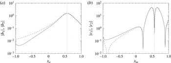
(a) Dependence of the absolute value of the control residuals
 $|b_{1}|$
(solid curve) and
 $|b_{2}|$
(dashed curve) on the actuator location
 $x_{a}$
in case #1. The maxima of the residuals
 $|b_{1}|$
and
 $|b_{2}|$
occur at
 $x_{a}=0.571$
and
 $x_{a}=0.564$
, respectively. The dotted vertical line indicates the
 $x$
-coordinate of the point-vortex equilibrium. (b) Same as (a), but for the observability residuals
 $|c_{1}|$
and
 $|c_{2}|$
. The maxima of the residuals
 $|c_{1}|$
and
 $|c_{2}|$
occur at
 $x_{m}=0.648$
and
 $x_{m}=0.487$
, respectively.

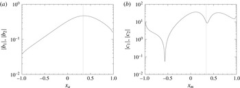
(a) Dependence of the absolute value of the control residuals
 $|b_{1}|$
and
 $|b_{2}|$
on the actuator location
 $x_{a}$
in case #2 (the values of
 $|b_{1}|$
and
 $|b_{2}|$
are essentially the same in this configuration). The maximum value of the control residuals occurs at
 $x_{a}=0.358$
. The dotted vertical line indicates the
 $x$
-coordinate of the point-vortex equilibrium. (b) Same as (a), but for the observability residual. Here the maximum value occurs at
 $x_{m}=0.113$
.

(a) Dependence of the absolute value of the control residuals
 $|b_{1}|$
and
 $|b_{2}|$
on the actuator location
 $x_{a}$
in case #3 (the values of
 $|b_{1}|$
and
 $|b_{2}|$
are essentially the same in this configuration). The maximum value of the control residuals occurs at
 $x_{a}=0.497$
. The dotted vertical line indicates the
 $x$
-coordinate of the point-vortex equilibrium. (b) Same as (a), but for the observability residual. Here the maximum value occurs at
 $x_{m}=0.413$
.

(a) Dependence of the absolute value of the control residuals
 $|b_{1}|$
and
 $|b_{2}|$
on the actuator location
 $x_{a}$
in case #4 (the values of
 $|b_{1}|$
and
 $|b_{2}|$
are essentially the same in this configuration). The maximum value of the control residuals occurs at
 $x_{a}=0.334$
. The dotted vertical line indicates the
 $x$
-coordinate of the point-vortex equilibrium. (b) Same as (a), but for the observability residual. Here the maximum value occurs at
 $x_{m}=0.087$
.

The dependence of the absolute values of the control residual on
 $x_{a}$
and observability residual on
 $x_{m}$
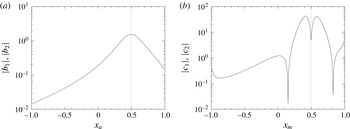
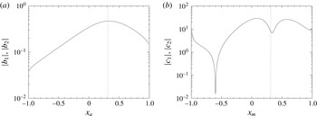
is shown for cases #1 and #2 in figures 6 and 7, and for cases #3 and #4 in figures 8 and 9. To obtain these figures, the coordinates
 $x_{a},x_{m}\in [-1,1]$
were discretized using 800 equispaced grid points and the residuals were evaluated at each point. Residuals for cases #5–7 produced similar features to those already presented in figures 6–9 and therefore, for brevity, the full details of these are excluded. In most cases the residuals of both modes are very similar and, in fact, for cases #2–6 the residuals are (to numerical tolerance) essentially the same. Only small differences between the residuals of the two modes are seen in cases #1 and #7. We remark that while the control residuals are in all cases bounded away from zero, the observability residuals may vanish at some isolated points. This occurs when the observability residuals
 $c_{1}$
and
 $c_{2}$
change sign and is manifested by ‘spikes’ visible in figures 6(b)–9(b) (due to numerical resolution, these spikes are smeared and do not actually reach zero). We therefore conclude that observability may be lost for some isolated sensor locations
 $x_{m}$
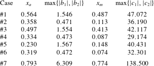
. In the results that follow, the actuator will be situated at the location
 $x_{a}$
corresponding to
 $\text{max}\{|b_{1}|,|b_{2}|\}$
and the sensor will be situated at
 $x_{m}$
corresponding to the maximum of the observation residuals
 $\text{max}\{|c_{1}|,|c_{2}|\}$
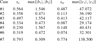
. A summary of the optimal locations of
 $x_{a}$
and
 $x_{m}$
for each configuration is shown in table 3.
Summary of the actuator and sensor placement in each case together with the corresponding maximum values of the controllability and observability residuals.
4 LQG control design
In this section the control algorithm is derived for the model system (3.14) based on linear optimal control theory (Stengel Reference Stengel1994). The derivation follows closely the approach implemented in Protas (Reference Protas2004). The objective is to find a feedback control law
 $m=-\unicode[STIX]{x1D646}\boldsymbol{X}^{\prime }$
, where
 $\unicode[STIX]{x1D646}$
is a
 $[2\times 1]$
feedback matrix, that will asymptotically stabilize system (3.14) while minimizing a performance criterion represented by the following cost functional
 $$\begin{eqnarray}{\mathcal{J}}(m):=\mathbb{E}\left[\int _{0}^{\infty }(YQY+mRm)\,\text{d}t\right],\end{eqnarray}$$
where
 $\mathbb{E}$
denotes the expectation, whereas
 $Q\geqslant 0$
and
 $R>0$
are given numbers. We note that the cost functional (4.1) balances the linearized system output
 $Y$
(i.e. the pressure difference across the wing) at the sensor location
 $(x_{m},0)$
, cf. (3.14b
), and the control effort, whereas the feedback control law provides a recipe for determining the actuation (i.e. the strength
 $m$
of the sink–source) based on the state of the linearized model (i.e. the perturbation
 $\boldsymbol{X}^{\prime }$
of the equilibrium). In practice, however, the state
 $\boldsymbol{X}^{\prime }$
of the model (3.14) is not known. Instead, noisy measurements
 ${\tilde{Y}}$
of the actual system (i.e. the nonlinear single-plate or Kasper wing system (3.1)) are available and can be used in an estimation procedure to construct an estimate
 $\boldsymbol{X}_{e}^{\prime }$
of the model state
 $\boldsymbol{X}^{\prime }$
. The evolution of the state estimate
 $\boldsymbol{X}_{e}^{\prime }$
is governed by the estimator system
 $$\begin{eqnarray}\displaystyle & \displaystyle \frac{\text{d}}{\text{d}t}\boldsymbol{X}_{e}^{\prime }=\unicode[STIX]{x1D63C}\boldsymbol{X}_{e}^{\prime }+m\unicode[STIX]{x1D63D}+\unicode[STIX]{x1D647}({\tilde{Y}}-Y_{e}), & \displaystyle\end{eqnarray}$$
 $$\begin{eqnarray}\displaystyle & \displaystyle Y_{e}=\unicode[STIX]{x1D63E}\boldsymbol{X}_{e}^{\prime }+mD, & \displaystyle\end{eqnarray}$$
 $\unicode[STIX]{x1D647}$
is a feedback matrix that will be chosen below in a manner ensuring that the estimation error vanishes in the infinite time horizon, i.e. that
 $\boldsymbol{X}_{e}^{\prime }\rightarrow \boldsymbol{X}^{\prime }$
as
 $t\rightarrow \infty$
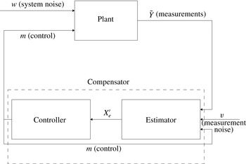
. Thus, the estimator assimilates available observations into the system model, so as to produce an evolving estimate of the system state. Finally, the controller and the estimator can be combined to form a compensator in which the feedback control is determined based on the state estimate
 $\boldsymbol{X}_{e}^{\prime }$
as
 $$\begin{eqnarray}m=-\unicode[STIX]{x1D646}\boldsymbol{X}_{e}^{\prime }.\end{eqnarray}$$
The flow of information in a compensator is shown schematically in figure 10.
Schematic of a compensator composed of an estimator and a controller.

The design of a LQG compensator can be accomplished using standard methods of linear control theory (see, e.g. Stengel Reference Stengel1994) and is outlined below only briefly. Assuming that all the stochastic variables are white and Gaussian, the separation principle can be applied which means that the control and estimation problems can be solved independently of each other. Based on the above assumptions, solution of the control problem can be further simplified by invoking the principle of certainty equivalence stating that the optimal feedback matrix
 $\unicode[STIX]{x1D646}$
for the stochastic system (3.14) with the cost function (4.1) is exactly the same as for the corresponding deterministic system obtained by setting the stochastic disturbance
 $w$
to zero. The matrix
 $\unicode[STIX]{x1D646}$
is then determined via
 $$\begin{eqnarray}\unicode[STIX]{x1D646}=\frac{1}{R}\unicode[STIX]{x1D63D}^{\text{T}}\unicode[STIX]{x1D64B}\end{eqnarray}$$
in which the
 $1\times 2$
matrix
 $\unicode[STIX]{x1D64B}$
is a symmetric positive-definite solution of the algebraic Riccati equation
 $$\begin{eqnarray}\unicode[STIX]{x1D63C}^{\text{T}}\unicode[STIX]{x1D64B}+\unicode[STIX]{x1D64B}\unicode[STIX]{x1D63C}+Q\,\unicode[STIX]{x1D63E}^{\text{T}}\unicode[STIX]{x1D63E}-\frac{1}{R}\unicode[STIX]{x1D64B}\unicode[STIX]{x1D63D}\unicode[STIX]{x1D63D}^{\text{T}}\unicode[STIX]{x1D64B}=\mathbf{0}.\end{eqnarray}$$
We note that the feedback matrix
 $\unicode[STIX]{x1D646}$
will depend on the choice of the output weight
 $Q$
and the control penalty
 $R$
in the cost functional (4.1). The optimal estimator feedback matrix needed in (4.2a
) is given by
 $$\begin{eqnarray}\unicode[STIX]{x1D647}=\frac{1}{M}\unicode[STIX]{x1D64E}\unicode[STIX]{x1D63E}^{\text{T}},\end{eqnarray}$$
where the matrix
 $\unicode[STIX]{x1D64E}$
is a symmetric positive-definite solution of the algebraic Riccati equation
 $$\begin{eqnarray}\unicode[STIX]{x1D63C}\unicode[STIX]{x1D64E}+\unicode[STIX]{x1D64E}\unicode[STIX]{x1D63C}^{\text{T}}+W\unicode[STIX]{x1D642}\unicode[STIX]{x1D642}^{\text{T}}-\frac{1}{M}\unicode[STIX]{x1D64E}\unicode[STIX]{x1D63E}^{\text{T}}\unicode[STIX]{x1D63E}\unicode[STIX]{x1D64E}=\mathbf{0},\end{eqnarray}$$
in which the disturbance structure is assumed to be
 $\mathbb{E}[w(t)w(\unicode[STIX]{x1D70F})^{\text{T}}]=W\unicode[STIX]{x1D6FF}(t-\unicode[STIX]{x1D70F})$
and
 $\mathbb{E}[v(t)v(\unicode[STIX]{x1D70F})^{\text{T}}]=M\unicode[STIX]{x1D6FF}(t-\unicode[STIX]{x1D70F})$
. Thus, the optimal estimator feedback
 $\unicode[STIX]{x1D647}$
depends on the covariances of the system and measurement disturbances,
 $W$
and
 $M$
, respectively, and yields an estimator known as the Kalman filter. For the case of the simple point-vortex models studied here, the algebraic Riccati equations (4.5) and (4.7) can be solved using standard techniques. As a matter of fact, equation (4.5) represents a system of three coupled quadratic equations and can be reduced to a scalar quartic equation that, in principle, can be solved in closed form. However, the analytic expressions obtained are prohibitively complicated and in practice it is much more convenient to use a numerical solution provided by the control toolbox in Matlab (MathWorks Reference Mathworks2014).
The LQG compensator is an example of an
 ${\mathcal{H}}_{2}$
controller / estimator design in which disturbances are assumed Gaussian and uncorrelated with the state and control. Robustness of the compensator can be enhanced by performing an
 ${\mathcal{H}}_{\infty }$
controller / estimator design where disturbances are allowed to have the worst case form. In the present study, however, the point-vortex model has a very simple structure and robustness can be achieved by hand tuning the compensator. Consequently, we do not pursue the
 ${\mathcal{H}}_{\infty }$
compensator design here and refer the reader to the review paper of Bewley (Reference Bewley2001) for a discussion of the utility of the
 ${\mathcal{H}}_{\infty }$
design in the context of flow control problems.
5 Numerical results: deterministic setting
In this section we present computational results in which LQG-based feedback stabilization is added to the base flow. The configurations to be examined were previously introduced in table 2, labelled cases #1–7.
Integration of (3.1) was again carried out using Euler’s explicit method with a time step of
 $\text{d}t=0.001$
. This time step was chosen as it is sufficiently small for a wide range of cases. Larger time steps are suitable in many situations, except that when the vortex passes close to a plate a small time step is required. In the solution of the estimation problem (4.2) it was assumed that the covariances of the plant and measurement disturbances were given by
 $$\begin{eqnarray}W=1.0,\quad M=1.0.\end{eqnarray}$$
Unless otherwise stated, in the solution of the control problem (4.5) we chose
 $$\begin{eqnarray}R=1.0,\quad Q=1.0.\end{eqnarray}$$
Initially, small perturbations of the equilibrium vortex positions will be considered to demonstrate that the control is successful in each of the chosen cases. Following this, the range of perturbations for which the control succeeds in stabilizing the equilibrium will be examined in each case.
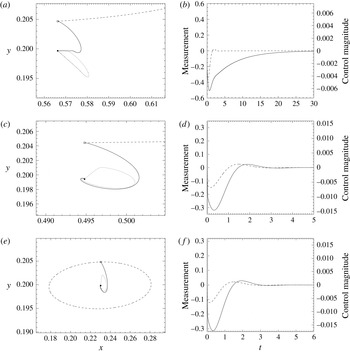
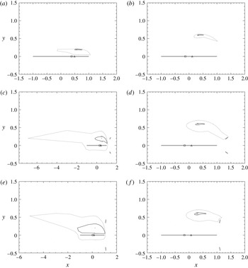
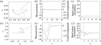
The first, second and third row correspond to cases #1, #3 and #5: (a,c,e) the uncontrolled vortex trajectory is represented by the dashed curve, the trajectory with LQG-based stabilization by the solid curve and the estimator trajectory by the dotted curve. The solid circular symbol represents the unperturbed equilibrium position and the square the initial perturbed position. (b,d,f) The corresponding linearized measurement
 $Y(t)$
(solid curve) and control intensity
 $m(t)$
(dashed curve).

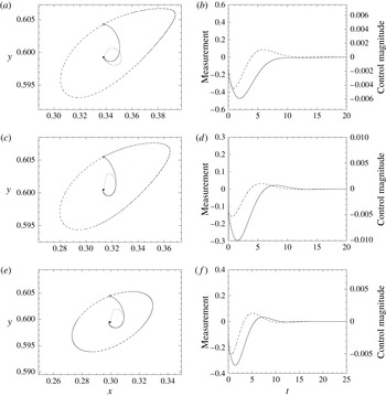
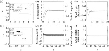
The first, second and third row correspond to cases #2, #4 and #6: (a,c,e) the uncontrolled vortex trajectory is represented by the dashed curve, the trajectory with LQG-based stabilization by the solid curve and the estimator trajectory by the dotted curve. The solid circular symbol represents the unperturbed equilibrium position and the square the initial perturbed position. (b,d,f) The corresponding linearized measurement
 $Y(t)$
(solid curve) and control intensity
 $m(t)$
(dashed curve).

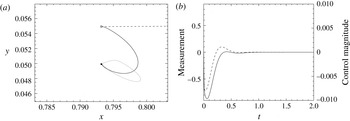
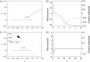
Case #7: (a) the uncontrolled vortex trajectory is represented by the dashed curve, the trajectory with LQG-based stabilization by the solid curve and the estimator trajectory by the dotted curve. The solid circular symbol represents the unperturbed equilibrium position and the square the initial perturbed position. (b) The corresponding measurement
 $Y(t)$
(solid curve) and control intensity
 $m(t)$
(dashed curve).

Figures 11–13 correspond to cases #1–7 in which the vortex is initially perturbed by
 $\unicode[STIX]{x1D6FF}=0.005\text{i}$
away from its equilibrium position
 $z_{\unicode[STIX]{x1D6FC}}$
(see table 2). For these small perturbations, and with LQG stabilization added, the trajectories in all cases are stabilized and the vortex position approaches
 $z_{\unicode[STIX]{x1D6FC}}$
as
 $t\rightarrow \infty$
. However, the time frame over which stabilization occurs, evident in the time-varying control intensity
 $m(t)$
, differs between cases. As regards case #3, we note that the trajectory in the uncontrolled configuration diverges (figure 11
c), even though the equilibrium is neutrally stable, cf. table 2. This is because in this case the magnitude of the initial perturbation
 $\unicode[STIX]{x1D6FF}$
is already outside the range of validity of linearization. From a practical point of view, it is pertinent to compare cases in which the vortex equilibrium is at the same elevation above the plate, i.e. cases #1, #3 and #5, and cases #2, #4 and #6. Letting the current vortex position be
 $z(t;\unicode[STIX]{x1D6FF})$
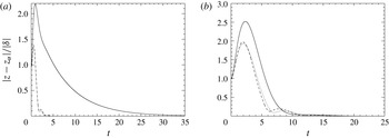
, figure 14(a,b) show the time evolution of the magnitude of the normalized perturbation (given by
 $|z(t;\unicode[STIX]{x1D6FF})-z_{\unicode[STIX]{x1D6FC}}|/|\unicode[STIX]{x1D6FF}|$
). Figure 14(a) shows clearly that the two neutrally stable configurations (cases #3 and #5) are stabilized far quicker than the unstable configuration (case #1). In the neutrally stable cases #2, #4 and #6, shown in figure 14(b), stabilization occurs over a similar time frame but it is notable that in the single-plate configuration (case #2) the perturbation exhibits a far greater transient growth prior to successful stabilization. It is also noted that an initial ‘kick’ is seen in the estimator trajectories and is particularly evident in the trajectories shown in figure 12 when the vortex has a larger circulation. This kick is due to the initial perturbation of the vortex location which is not accounted for in the initial condition of the estimator (
 $\boldsymbol{X}_{e}^{\prime }(0)=\mathbf{0}$
in (4.2a
)).
Time evolution of the magnitude of the perturbation for: (a) case #1 (solid curve), case #3 (dotted curve) and case #5 (dashed curve), (b) case #2 (solid curve), case #4 (dotted curve) and case #6 (dashed curve).

(a–f) Basins of attraction for cases #1–6 respectively. Thick solid lines represent the plates, dotted curves the basins when
 $R=1$
and solid curves the basins when
 $R=100$
(cf. (4.1)). The actuator and sensor locations are indicated by the triangle and square symbols respectively.

Case #5 with an initial perturbation of
 $\unicode[STIX]{x1D6FF}=-2.0$
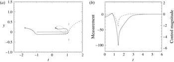
. (a) The vortex trajectory with LQG-based stabilization is represented by the solid curve, the estimator trajectory by the dotted curve and the uncontrolled trajectory by the dashed curve. The solid circular symbol represents the unperturbed equilibrium position and the square the initial perturbed position. (b) The corresponding measurement
 $Y(t)$
(solid curve) and control intensity
 $m(t)$
(dashed curve).

To explore the range of perturbations for which LQG stabilization is successful in each case, ‘basins of attraction’ are computed. They represent the sets of initial perturbations which can be stabilized by the LQG compensator; trajectories corresponding to perturbations lying outside these basins escape to infinity. Each basin is computed by discretizing perturbations
 $\unicode[STIX]{x1D6FF}\in \mathbb{C}$
about
 $z_{\unicode[STIX]{x1D6FC}}$
such that
 $$\begin{eqnarray}\unicode[STIX]{x1D6FF}_{j}=r_{j}\text{e}^{2\unicode[STIX]{x03C0}\text{i}(j/J)},\quad j=0,\ldots ,J-1,\end{eqnarray}$$
where
 $r_{j}\in \mathbb{R}$
and
 $J=100$
. The algorithm then calculates, for each
 $j$
, the largest value of
 $r_{j}$
(to within an accuracy of 0.01) such that
 $|z(t;\unicode[STIX]{x1D6FF}_{j})-z_{\unicode[STIX]{x1D6FC}}|\rightarrow 0$
as
 $t\rightarrow \infty$
. Additionally, to demonstrate the effect of changing the cost of control (see (4.4)), basins are computed for both
 $R=1$
and
 $R=100$
. When
 $R=1$
control is ‘cheap’ and can be used liberally. However, when the cost is increased to
 $R=100$
, control is ‘expensive’ and must be used sparingly. Therefore, for larger values of
 $R$
, the basins of attraction are expected to shrink. The basins computed for cases #1–6 are shown in figure 15. When comparing cases #1, #3 and #5, the basins of the two Kasper wing configurations (for both values of
 $R$
) are significantly larger than those of the single-plate configuration. Indeed, in cases #3 and #5 when
 $R=1$
, due to the trajectories the point vortex follows past the plates, the control is capable of stabilizing some extreme perturbations. For the equilibria further from the plate, basins of the Kasper wing cases #4 and #6 are still noticeably larger than those of the single-plate case #2, but now to a lesser extent. It should also be pointed out that in cases #3 and #5 the basin ‘engulfs’ the main plate. However, as the vortex approaches the plate boundary, the expression in (2.2) becomes singular and the numerical computations are no longer robust. Perturbations placing the vortex very close to one of the plates cannot therefore be claimed to be part of a basin of attraction. Finally in this section, figure 16 presents a vortex trajectory together with the corresponding time histories of the linearized measurements
 $Y(t)$
and control intensity
 $m(t)$
for a large perturbation in case #5. This example shows one of the more ‘exotic’ trajectories the LQG control is capable of stabilizing in which the vortex moves away from the equilibrium and passes under the plate prior to the control latching onto it and ‘pulling’ it towards the equilibrium.
6 Numerical results: effects of disturbances
In this section we examine how the LQG control performs in the presence of additional disturbances affecting the flow. Two forms of disturbances are independently considered: the first of these will be random disturbances added to the angle of attack
 $\unicode[STIX]{x1D712}_{0}$
of the oncoming flow and then a vortex-shedding model will be introduced ensuring that the Kutta conditions (see (2.10a
)–(2.10c
)) are satisfied at discrete instances of time throughout a simulation. Needless to say, the phenomenon of vortex shedding is not accounted for in the flow model (cf. § 2) and hence may be interpreted as ‘system uncertainty’. Therefore, even though it is deterministic in nature, it may be represented by the term proportional to
 $w$
in (3.14a
). Details concerning the two forms of disturbances are discussed in their respective subsections below.
6.1 Control in the presence of random disturbances of the angle of attack
To check how the control performs in a fluctuating background flow, the flow angle of attack
 $\unicode[STIX]{x1D712}_{0}$
is periodically augmented with a Gaussian random variable, so that we obtain
 $$\begin{eqnarray}\unicode[STIX]{x1D712}(t)=\unicode[STIX]{x1D712}_{0}+\unicode[STIX]{x0394}\unicode[STIX]{x1D712}\left(\left\lfloor \frac{t}{\unicode[STIX]{x0394}t}\right\rfloor \right),\end{eqnarray}$$
where
 $\unicode[STIX]{x0394}t=0.01$
,
 $\lfloor \cdot \rfloor$
denotes the integer part and
 $\unicode[STIX]{x0394}\unicode[STIX]{x1D712}(l)$
is the
 $l$
th sample of the random variable with distribution
 ${\mathcal{N}}(\unicode[STIX]{x1D707},\unicode[STIX]{x1D70E}^{2})$
for some
 $\unicode[STIX]{x1D70E},\unicode[STIX]{x1D707}\in \mathbb{R}$
. In other words, the stochastic disturbance is frozen over the time window of length
 $\unicode[STIX]{x0394}t$
before a new sample is drawn. We are interested here in a single realization of the stochastic process, rather than in any statistic quantities, so once the random variable has been sampled, the closed-loop system (3.1) with (6.1) can be integrated as a deterministic system. We do so with the approach introduced in § 5, i.e. Euler’s explicit method with the time step
 $\text{d}t=0.001$
.
In figure 17 we show the vortex trajectories together with the corresponding histories of the measurements and control intensities obtained for disturbances with
 $\unicode[STIX]{x1D707}=0$
and two different values of
 $\unicode[STIX]{x1D70E}^{2}$
(0.2 and 0.4). In both these examples the initial perturbation has been chosen to lie close to the edge of the basin of attraction and in the absence of control the corresponding vortex trajectories are swept to infinity. For these relatively large perturbations it is seen that the control still performs well in the presence of a fluctuating background flow, even for large values of
 $\unicode[STIX]{x1D70E}^{2}$
. Figure 18 then presents two examples corresponding to cases #1 and #5 from table 2 with disturbances for which
 $\unicode[STIX]{x1D707}>0$
. In both these cases,
 $\unicode[STIX]{x0394}\unicode[STIX]{x1D712}\sim {\mathcal{N}}(0.1,0.1)$
in (6.1) and the same initial perturbation with
 $\unicode[STIX]{x1D6FF}=-0.25$
was used, chosen to lie within each of the respective basins of attraction. In the single-plate configuration (figure 18
a,b) the control fails and the vortex quickly escapes. However, in the Kasper wing configuration (figure 18
c,d) the control is robust and the vortex gradually moves to, and then undergoes a random motion about, a point close to the uncontrolled equilibrium. We note that in case #5 in the absence of control the vortex trajectory also remained bounded, although in comparison with the controlled case, the departures from the equilibrium position were much larger (to avoid cluttering figures, these results are not shown here).
Figures 17 and 18 illustrate representative types of behaviour seen in the presence of the stochastic forcing in the form (6.1). The general behaviour can be summarized as follows. When
 $\unicode[STIX]{x1D707}$
was set to zero, the closed-loop control system was robust with respect to stochastic disturbances (6.1) in all cases considered, even for large values of
 $\unicode[STIX]{x1D70E}^{2}$
. Perturbed trajectories would eventually perform a ‘random walk’ in a region near the uncontrolled equilibrium whose extent depends on
 $\unicode[STIX]{x1D70E}^{2}$
and in this regime the control magnitude oscillates around zero. On the other hand, for values of
 $\unicode[STIX]{x1D707}>0$
the closed-loop control was unable to stabilize the equilibrium in cases #1 and #2 even for small values of
 $\unicode[STIX]{x1D707}$
. However, in cases #3–6 it remained robust up to larger values of
 $\unicode[STIX]{x1D707}$
.
(a) Vortex trajectories (solid curve) and estimator trajectories (dotted curve) for initial perturbation
 $\unicode[STIX]{x1D6FF}=-0.1\text{i}$
and disturbances with
 $\unicode[STIX]{x0394}\unicode[STIX]{x1D712}\sim {\mathcal{N}}(0,0.2)$
in a case #1. The square symbol indicates the initial position of the perturbed vortex and the solid circle the equilibrium position in the absence of any stochastic forcing. (b) The corresponding time histories of the measurement (solid curve) and control magnitude (dashed curve). (c,d) Same as (a,b), but for a case #4 configuration with
 $\unicode[STIX]{x1D6FF}=0.075\text{i}$
and
 $\unicode[STIX]{x0394}\unicode[STIX]{x1D712}\sim {\mathcal{N}}(0,0.4)$
; in (c) the inset represents a magnification of the neighbourhood of the equilibrium.

(a) Vortex trajectories (solid curve) and estimator trajectories (dotted curve) for initial perturbation
 $\unicode[STIX]{x1D6FF}=-0.25$
and disturbances with
 $\unicode[STIX]{x0394}\unicode[STIX]{x1D712}\sim {\mathcal{N}}(0.1,0.1)$
in a case #1. The square symbol indicates the initial position of the perturbed vortex and the solid circle the equilibrium position in the absence of any stochastic forcing. (b) The corresponding time histories of the measurement (solid curve) and control magnitude (dashed curve). (c,d) Same as (a,b), but for a case #5. The inset in (c) shows a magnification of the region close the uncontrolled vortex equilibrium.

6.2 Control in the presence of vortex shedding
We now augment our model with a vortex-shedding mechanism in which point vortices are ‘injected’ into the flow at locations close to the rear tips of each plate at discrete instances of time. The circulations of these injected vortices are chosen such that the Kutta condition (2.10c
) at the rear tip of each plate is satisfied at the time of injection. Integration is again carried out using Euler’s explicit method with a time step of
 $\text{d}t=0.001$
. Vortices are injected into the flow at
 $t=0$
and then at intervals of
 $\unicode[STIX]{x0394}t=0.1$
. The injection location is chosen to be at a distance of
 $0.1$
from each plate tip in the direction tangent to the plate. That is, in cases #1–6 a single vortex is injected at the point
 $$\begin{eqnarray}z_{i1}=1+0.1=1.1.\end{eqnarray}$$
Additionally, in cases #3–6 two further vortices are injected at
 $$\begin{eqnarray}\displaystyle & \displaystyle z_{i2}=1+(0.45+0.1)\text{e}^{\text{i}\unicode[STIX]{x1D719}}, & \displaystyle\end{eqnarray}$$
 $$\begin{eqnarray}\displaystyle & \displaystyle z_{i3}=\overline{z_{i2}}. & \displaystyle\end{eqnarray}$$
(a) Case #1 configuration with initial perturbation
 $\unicode[STIX]{x1D6FF}=0.3$
. The dashed curve represents the controlled vortex trajectory starting from the outside of the basin of attraction in the absence of shedding, the thin solid curve the controlled trajectory in the presence of shedding and the dotted curve the estimator trajectory in the presence of shedding. The solid circular symbol represents the unperturbed equilibrium position and the square the initial perturbed position. (b) The corresponding time history of the measurements
 $Y(t)$
(solid curve) and control intensity
 $m(t)$
(dashed curve) in the presence of shedding. (c) The corresponding circulation of the most recently shed vortex at
 $z_{i1}$
. (d–f) Same as (a–c) but for a case #5 configuration with
 $\unicode[STIX]{x1D6FF}=0.52\text{i}$
. Additionally, in (d) the thicker solid lines represent the plate boundaries and in (f) the solid, dotted and dashed curves represents the circulations of the most recently shed vortices at
 $z_{i1}$
,
 $z_{i2}$
and
 $z_{i3}$
respectively.

Examples of the various behaviours observed with vortex shedding added are presented in figures 19 and 20. These behaviours can be summarized as follows. In general, the addition of shed vortices has a stabilizing effect. In almost all configurations tested, perturbations larger than those in the absence of shedding could be stabilized (exceptions to this rule will be mentioned below and are discussed in a little further detail in the following section). In figure 19, two examples are shown in which the vortex is initially perturbed to outside the basins of attraction determined in § 5. Despite this, the vortex trajectories are rapidly stabilized and, after an initial increase, the circulations of the most recently shed vortices decay to zero as demonstrated in figure 19(c,f).
Figure 20(a–c) demonstrates a slightly different behaviour. Now, owing to the larger circulation of the point vortex, instead of returning to the unperturbed equilibrium position, the vortex is held at a location close to the equilibrium and the circulations of the shed vortices tend to constant values. That is, a new equilibrium state emerges. Finally, figure 20(d–f) shows an example of a ‘chaotic’ case. In situations where the perturbation
 $\unicode[STIX]{x1D6FF}$
is too large for the vortex to be stabilized, but not large enough for the vortex to escape, the vortex can undergo a complicated motion in the vicinity of the equilibrium location over a long period of time.
Although the presence of vortex shedding has, in general, a stabilizing effect in the majority of cases, two scenarios were identified in which the effect was in fact destabilizing. Firstly, in the configurations corresponding to case #2 equilibria would not be stabilized for any initial perturbation
 $\unicode[STIX]{x1D6FF}$
. Additionally, in cases #3–6 when an initial perturbation with a large positive real component is taken, the extent to which the corresponding evolutions can be controlled is reduced. Physical arguments for these scenarios are discussed in the following section.
(a) Case #4 configuration with initial perturbation of
 $\unicode[STIX]{x1D6FF}=0.1\text{i}$
. The dashed curve represents the controlled vortex trajectory in the absence of shedding, the thin solid curve the controlled trajectory in the presence of shedding and the dotted curve the estimator trajectory in the presence of shedding. The thicker solid lines represent the plate boundaries, the solid circular symbol the unperturbed equilibrium position and the square the initial perturbed position. The inset shows a magnification of the region close the vortex equilibrium. (b) The corresponding time histories of the measurements
 $Y(t)$
(solid curve) and control intensity
 $m(t)$
(dashed curve) in the presence of shedding. (c) The corresponding circulations of the most recently shed vortices at
 $z_{i1}$
(solid curve),
 $z_{i2}$
(dotted curve) and
 $z_{i3}$
(dashed curve). (d–f) Same as (a–c) but for a case #1 configuration with
 $\unicode[STIX]{x1D6FF}=0.375\exp (-0.13\text{i}\unicode[STIX]{x03C0})$
. The inset shows the region close to the unperturbed equilibrium.

7 Discussion
Before concluding, results presented in this paper are briefly summarized and some additional points of discussion are raised. First, from a control design perspective, for the given choice of actuation mechanism (sink–source singularity) and measurement (pressure difference across the main plate), all configurations demonstrated a similar responsiveness. That is, the chosen configurations were completely controllable and observable for all sensor and actuator locations and the corresponding residuals displayed the same general features.
Placing the sink–source actuator at the location with maximal controllability residual and the pressure sensor at the location with maximal observability, the control was seen to be effective for a range of perturbations in all cases considered. Also, as demonstrated in figure 14(a), for comparable setups neutrally stable configurations could be stabilized in a shorter amount of time than linearly unstable configurations. The range of perturbations for which the control was effective varied from cases to case. Not unexpectedly, for a given configuration, a larger range of perturbations could be stabilized when the vortex equilibrium was located closer to the main plate. Such equilibria are comprised of vortices with a weaker circulation and they are therefore more easily influenced by the sink–source actuator. However, whilst it was expected that the presence the auxiliary ‘flaps’ in Kasper wing configurations would enhance the robustness of the control, the substantial increase in robustness was somewhat surprising, especially in cases #3 and #5. Indeed, at least in the inviscid setting, this demonstrates the large effect additional (small) boundaries can have on such flows. We add that a similar stabilizing effect achieved by a small obstacle placed in the wake of a larger body was observed experimentally by Strykowski & Sreenivasan (Reference Strykowski and Sreenivasan1990), and later explained in terms of intrinsic stability properties by Giannetti & Luchini (Reference Giannetti and Luchini2007).
The effectiveness of the control was then examined in the presence of additional disturbances designed to mimic the uncertainty of the flow model and the flow configuration. With a randomly varying angle of attack
 $\unicode[STIX]{x1D712}(t)$
, provided its mean value was unchanged and equal to
 $\unicode[STIX]{x1D712}_{0}$
, the system could be successfully controlled even for large oscillations of the angle of attack. In such cases, the vortex would undergo a random walk around its equilibrium location. On the other hand, as the expectation of the randomly perturbed angle of attack was allowed to deviate from
 $\unicode[STIX]{x1D712}_{0}$
, for which the LQG compensator was designed, the control would quickly fail (with single-plate configurations breaking down quicker than their Kasper wing counterparts). When a vortex-shedding model was introduced, the robustness of the control was seen to improve in all cases for almost all perturbations. An exception to this was when the vortex was perturbed downstream of the equilibrium position in Kasper wing configurations (figure 20
a–c). In such scenarios, pushing the vortex close to the rear tip of one of the three plates would result in three vortices with substantial circulations being shed and the system becoming unstable. Furthermore, with the addition of vortex shedding, new ‘exotic’ trajectories such as that presented in figure 20(d) could be observed. In that particular example, it appears that the vortex may enter a limit cycle around a new equilibrium. Finally, although not discussed in § 6.2, it is now noted that in the presence of shedding case #2 is seen to be uncontrollable for all perturbations. This can be understood by viewing the streamline pattern for this case shown in figure 5(b) in which the recirculation region of the vortex engulfs the plate. As a result, vortices are shed with far weaker circulations than that of the main vortex and are trapped in the recirculation region. This eventually leads to a build up of circulation around the plate, a state which cannot be effectively controlled. Indeed, it may be expected that this phenomenon will occur for any equilibrium in which the vortex recirculation region engulfs any boundary from which vortices are shed. The relation between detachment of the leading-edge vortex and the global flow topology in real flows was investigated experimentally by Rival et al. (Reference Rival, Kriegseis, Schaub, Widmann and Tropea2014) and using a vortex-based model by Ramesh et al. (Reference Ramesh, Gopalarathnam, Granlund, Ol and Edwards2014).
8 Conclusions
In this paper, an LQG compensator was designed to stabilize point-vortex equilibria located above both an inclined flat plate and Kasper wing in the presence of an oncoming uniform flow. A sink–source singularity placed on the main plate acted as the actuation mechanism and pressure difference across the main plate as the system output. Standard methods of linear control theory were used to characterize this flow model and the compensator was applied to a range of systems, the results of which are summarized in § 7. Other forms of actuation could also be considered, for example, applying an additional circulation around the main plate and details regarding the derivation of such alternative controls can be found in Protas (Reference Protas2004). However, the sink–source actuation was chosen for this study as its effect on the vortex can be considered analogous to that of a synthetic jet commonly used in similar studies in which viscosity is included (analogous models were also used to represent this form of flow actuation by Cortelezzi (Reference Cortelezzi1996), Zannetti & Iollo (Reference Zannetti and Iollo2003)).
A key result of our study is the demonstration of the large effect the addition of small boundaries has on the controlled flow. From a control design perspective, the effect of the Kasper flaps is to ‘push’ the vortex closer to the front of the plate and also slightly reduce its circulation (for vortex equilibria of corresponding elevation above the plate). Both these effects are beneficial in terms of the effectiveness of the control. Further, for nonlinearly unstable perturbations where in the absence of control the vortex quickly travels downstream (cf. figure 4 a), the flaps in general have the effect of slightly slowing down the escape. This is also beneficial in regard to the robustness of the control.
Inviscid flow models similar to that studied here have previously been considered as reduced-order models of real flows governed by the Navier–Stokes system (Protas Reference Protas2008). The simplicity of such reduced-order models, if they can be successfully utilized in the design a control strategy for the full model, is of course very appealing. In comparison to the study of Protas (Reference Protas2004), where a controller designed based on an inviscid Föppl vortex model was used to stabilize a bluff-body wake flow at
 $Re=75$
, applying the control strategy considered here to a flow governed by the full Navier–Stokes system will require some additional careful assumptions. This problem is currently being considered by the authors of this paper (along with additional collaborators) with the aim of implementing control approaches capable of stabilizing vortex configurations which concomitantly increase the lift and decrease the drag experienced by aerofoil configurations similar to those considered here. In particular, this investigation, which is based on the full Navier–Stokes model, will shed light on the significance of viscous effects always present in realistic flows, bringing in this way Kasper’s vision closer to fruition.
Acknowledgements
R.N. and T.S. would like to gratefully acknowledge the support of JST-CREST who helped fund this study. B.P. was supported through an NSERC (Canada) Discovery Grant. T.S. was partially supported by Grants-in-Aid for Scientific Research KAKENHI (B) no. 15TK0014 from JSPS.