1. Introduction
The Tutte polynomial packs a number of fundamental numerical graph invariants into a two-variable polynomial. It features heavily in modern graph theory and illuminates connections between it and other fields. Here we give a direct geometric argument relating it to important polynomial invariants in representation theory and geometry. We start by introducing our polynomials of interest and their mutual connections.
The Tutte polynomial of a graph  $\Gamma$ with edge set
 $E$ and vertex set
 $V$ is given by:
 \[ {\mathbf{T}}_{\Gamma}(x,y)=\sum \nolimits _{{D\subset E}}(x-1)^{{k(D)-k(E)}}(y-1)^{{k(D)+\#D-\#V}}, \]
where  $k(D)$ denotes the number of connected components of the subgraph of
 $\Gamma$ with edge set
 $D$. Tutte showed that
 $ {\mathbf {T}}_\Gamma$ has non-negative integer coefficients by expressing it as a sum over spanning trees
 $T \subset \Gamma$ as follows:
 \[ {\mathbf{T}}_\Gamma(x,y)=\sum_T x^{\operatorname{int}(\Gamma,T)}y^{\operatorname{ext}(\Gamma,T)}, \]
where  $\operatorname {int}(\Gamma ,\, T)$ and
 $\operatorname {ext}(\Gamma ,\,T)$ are integral weights attached to a spanning tree
 $T \subset \Gamma$ that depend on a fixed ordering of the set of edges
 $E$. Here we will only consider the specialization
 $ {\mathbf {T}}_\Gamma (1,\,q)$ and assume
 $\Gamma$ is connected, for which the two formulas above simplify respectively to
 \begin{align} {\mathbf{T}}_{\Gamma}(1,q)&=\sum_{{D\subset E\;\text{connected}}}(q-1)^{{1+\#D-\#V}}, \end{align}
 \begin{align} {\mathbf{T}}_{\Gamma}(1,q)&=\sum_{T} q^{\operatorname{ext}(\Gamma,T)}. \end{align}
The sum in (1.1) is over subsets  $D \subset E$ for which the subgraph of
 $\Gamma$ with edges
 $D$ is connected.
On the other hand, when the edges  $\Gamma$ are given an orientation, we may consider the indecomposable representations of the corresponding quiver
 $Q$. The polynomial counting the number of indecomposable representations of
 $Q$ over
 $ {\mathbb {F}}_q$ of dimension vector
 $ {\mathbf {v}}$ is called the Kac polynomial; we will use
 $A_ {\mathbf {v}}(q)$ to denote it. Throughout the introduction we will fix
 $ {\mathbf {v}}$ to be
 $(1,\,\ldots ,\,1)$ and call representations with this dimension vector toric representations. It is easy to deduce from (1.1) (see [Reference Hausel and Sturmfels6]) that the Kac polynomial satisfies
 \[ A_{\mathbf{v}}(q)={\mathbf{T}}_\Gamma(1,q). \]
So it is natural to ask for an interpretation of (1.2) in terms of the Kac polynomial.
Last but not least, is the Poincaré polynomial of the Nakajima quiver variety  $ {\mathcal {M}}:= {\mathcal {M}}_{\lambda , \theta }( {\mathbf {v}})$ with
 $ {\mathbf {v}}$ as above and
 $(\lambda ,\,\theta )$ generic hyperkähler parameters, where
 $\lambda \in {{\boldsymbol {k}}}^{Q_0}$ and
 $\theta \in {\mathbb {R}}^{Q_0}$. Definition 2.1 spells out what we mean by generic. According to general theory developed in [Reference Crawley-Boevey and Van den Bergh3], the Kac polynomial equals the Poincaré polynomial of the associated Nakajima quiver variety
 $ {\mathcal {M}}$ up to a power of
 $q$. The proof however uses deep geometric arguments, and in particular does not produce a direct interpretation of the formula (1.2).
In this work, we directly connect both the Kac polynomial and the Poincaré polynomial of the Nakajima variety to the Tutte polynomial using the formula (1.2). More precisely, given an ordering on  $E$, we show that spanning trees of
 $\Gamma$ naturally index both subsets of indecomposable representations of
 $Q$ and cells in a cell decomposition of
 $ {\mathcal {M}}$. For each tree
 $T$, the number of indecomposable representations of
 $Q$ in the corresponding subset is
 $q^{\operatorname {ext}(\Gamma , T)}$, while the corresponding cell
 $ {\mathcal {M}}_T\subset {\mathcal {M}}$ is isomorphic to
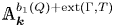 $ {\mathbb {A}}_{{{\boldsymbol {k}}}}^{b_1(Q)+\operatorname {ext}(\Gamma ,T)}$. See equations (1.3) and (2.1) for definitions of
 $\operatorname {ext}(\Gamma ,\, T)$ and
 $b_1(Q)$, respectively.
The Nakajima quiver variety  $ {\mathcal {M}}$ parametrizes stable representations of the double quiver associated with
 $Q$, which for every edge
 $e$ of
 $Q$ contains the opposite edge
 $e^{*}$. By forgetting the maps attached to the new edges
 $e^{*}$, each point of
 $ {\mathcal {M}}$ produces a representation of
 $Q$. So one can try to construct a cell decomposition of
 $ {\mathcal {M}}$ in such a way that a point of
 $ {\mathcal {M}}$ belongs to the cell indexed by a particular tree
 $T$ precisely when the corresponding representation of
 $Q$ belongs to the subset labelled by
 $T$. This idea does produce a nice cell decomposition in the case
 $\theta =0$ and
 $\lambda$ is generic. However, as soon as
 $\lambda =0$ and a non-trivial stability condition
 $\theta$ is involved, this naive approach does not work; for instance, the corresponding representation of
 $Q$ may fail to be indecomposable. So we need a more subtle construction.
Our proof goes through ‘geometrizing’ the deletion/contraction operators on graphs and spanning trees. The external activity of a spanning tree  $T$ may be expressed using a deletion/contraction recursion as follows: fix an ordering on
 $E$, for
 $e \in E$ the biggest non-loop edge we have:
 \begin{equation} \operatorname{ext}(\Gamma,T) = \begin{cases} \operatorname{ext}(\,{\Gamma\backslash e, T}\,) & \text{if } e \notin T \\ \operatorname{ext}(\,{\Gamma/e, T/e}\,) & \text{if } e \in T.\end{cases} \end{equation}
The base case is when  $\Gamma$ has exactly one vertex, we then set
 $\operatorname {ext}({\Gamma ,\,T})=\#E.$ This expression of
 $\operatorname {ext}(\Gamma ,\, T)$ has its roots in the beautifully efficient expression of the Tutte polynomial through a deletion/contraction recursion. For a good introduction to the Tutte polynomial from this perspective the reader may consult [Reference Coutinho1].
To ‘geometrize’ we begin by indexing points of  $ {\mathbf {p}} \in {\mathcal {M}}$ by trees. This indexing process is somewhat delicate: we use the stability parameter
 $\theta \in {\mathbb {R}}^{Q_0}$ to orient a given spanning tree and give an algorithm that would pick the ‘biggest’ amongst those whose oriented arrows are non-zero in
 $ {\mathbf {p}}$. One of the subtleties here is that
 $\theta$ may orient a given edge
 $e$ of
 $Q$ in one direction when
 $e$ is viewed as an edge of a spanning tree
 $T$, while orienting it in the opposite direction when
 $e$ is seen as an edge of a different spanning tree
 $T'$. Furthermore, the partial ordering in which the tree assigned to
 $ {\mathbf {p}}$ is the ‘biggest’ is not the lexicographic ordering induced by the ordering on the edges of
 $\Gamma$. See § 5 for an example in which both of these subtleties are displayed.
This indexing process gives a cell decomposition of  $ {\mathcal {M}}$. We then define deletion/contraction operators on the tree-indexed cells of
 $ {\mathcal {M}}$ to yield isomorphisms:
 \[ {\mathcal{M}}_T \simeq \begin{cases} (\,{\mathcal{M}}\backslash e\,)_T \times {\mathbb{A}}_{{\boldsymbol{k}}}^{1} & \text{if } e \notin T \\ (\,{\mathcal{M}}/ e\,)_{T/e} & \text{if } e \in T.\end{cases} \]
This is the content of our main theorems, theorems 4.16 and 4.18. The base case is again one where our quiver has one vertex, in that case 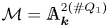 $ {\mathcal {M}} = {\mathbb {A}}_{{\boldsymbol {k}}}^{2(\#Q_1)}$.
The number of times the contraction operator is used to get to the base case is  $\#Q_0-1$. Therefore the number of times deletion is used to get to the base case is
 $\#Q_1-(\#Q_0-1) - \operatorname {ext}(\Gamma ,\,T)$. This may be written as
 $b_1(Q)-\operatorname {ext}(\Gamma ,\, T)$. We then have that
 \[ {\mathcal{M}}_T \simeq {\mathbb{A}}_{{\boldsymbol{k}}}^{2 \operatorname{ext}(\Gamma,T)} \times {\mathbb{A}}_{{\boldsymbol{k}}}^{b_1(Q)- \operatorname{ext}(\Gamma, T)} \simeq {\mathbb{A}}_{{\boldsymbol{k}}}^{b_1(Q)+\operatorname{ext}(\Gamma,T)}. \]
Hence we have the following expression for the Poincaré polynomial of  $ {\mathcal {M}}$:
 \[ P_{\mathcal{M}}(q) = q^{b_1(Q)} \cdot {\mathbf{T}}_Q(1,q). \]
This is restated in corollary 4.20.
The contents of this article are organized as follows. We start by setting up the notation and relevant background in § 2. We then go on to framing the classical results relating the Tutte polynomial and Kac polynomial in our context in § 3. In § 4, we address the main content of this work; we define a cell decomposition of  $ {\mathcal {M}}$ indexed by trees and use it to relate the Poincaré polynomial of
 $ {\mathcal {M}}$ to the Tutte polynomial. We finish off with a worked example in § 5.
2. Background and notation
2.1 Quivers
A quiver  $Q$ is specified by two finite sets
 $Q_0$ and
 $Q_1$ together with two maps
 $h,\, t \colon Q_1 \rightarrow Q_0$. We call the elements of these sets vertices and edges, respectively. The maps
 $h$ and
 $t$ indicate the vertices at the head and tail of each edge. A non-trivial path in
 $Q$ is a sequence of edges
 $p = e_1 \dotsb e_m$ with
 $h(e_{k}) = t(e_{k+1})$ for
 $1 \leq k < m$. We set
 $t(p) = t(e_{1})$ and
 $h(p)= h(e_m)$. For each
 $i \in Q_0$ we have a trivial path
 $ {\mathbf {e}}_i$ where
 $t( {\mathbf {e}}_i) = h( {\mathbf {e}}_i) = i$. The path algebra
 ${{\boldsymbol {k}}}Q$ is the
 ${{\boldsymbol {k}}}$-algebra whose underlying
 ${{\boldsymbol {k}}}$-vector space has a basis consisting of paths in
 $Q$; the product of two basis elements equals the basis element defined by concatenation of the paths if possible or zero otherwise. A cycle is a path
 $p$ in which
 $t(p) = h(p)$. From now on and for simplicity, we will assume that
 $Q$ is connected. A spanning tree
 $T$ is a connected subquiver that contains all the vertices with the minimal number of edges
 $\#Q_0-1$. The first Betti number of a quiver is given by
 \begin{equation} b_1(Q):= \#Q_1 - \#Q_0 + 1. \end{equation}
For a commutative ring  $R$, the
 $R$-module of functions
 $Q_0 \rightarrow R$ will be denoted
 $R^{Q_0}$. The double quiver
 ${{\overline {Q}}}$ associated to
 $Q$ is the quiver given by adjoining an extra edge of the opposite orientation for each edge
 $e \in Q_1$, that is
 ${{\overline {Q}}}_0 = Q$ and
 ${{\overline {Q}}}_1= Q_1 \cup (Q^{\text{op}})_1$. The edge of
 ${{\overline {Q}}}$ corresponding to the opposite of
 $e \in Q_1$ will be called
 $e^{*}$.
Given a non-loop edge  $e \in Q_1$ we define the contracted quiver
 $Q/e$ as follows. The vertices are given by
 $(Q/e)_0 = (Q_0 \setminus \{t(e),\,h(e)\}) \cup \{\iota \}$ and the edges by
 $(Q/e)_1 = Q_1 \setminus \{e\}$. Let
 $\alpha$ be the inclusion
 $(Q/e)_1$ in
 $Q_1$ and
 $\beta$ be the natural map
 $\beta \colon Q_0 \rightarrow (Q/e)_0$ taking both
 $t(e),\,h(e)$ to
 $\iota$. The head and tail maps
 $h',\,t' \colon (Q/e)_1 \rightarrow (Q/e)_0$ are given by pre-composing
 $h,\,t$ on
 $Q$ with
 $\alpha$ and post-composing with
 $\beta$. A spanning tree
 $T \subset Q$ naturally defines a spanning tree
 $T/e$ of
 $Q/e$ for any given edge
 $e\in T$. Furthermore, given an element
 $\lambda \in {{\boldsymbol {k}}}^{Q_0}$, we define
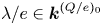 $\lambda /e \in {{\boldsymbol {k}}}^{(Q/e)_0}$ to take the value
 $\lambda (i)$ at
 $i \in (Q/e)_0 \setminus \{\iota \}$ and
 $(\lambda /e)(\iota ):=\lambda (h(e))+\lambda (t(e))$. Given
 $\theta \in {\mathbb {R}}^{Q_0}$ we define
 $\theta /e \in {\mathbb {R}}^{{Q/e}_0}$ in a similar fashion. We will drop the contraction notation ‘
 $/e$’ from subquivers, subtrees,
 ${{\boldsymbol {k}}}^{Q_0}$,
 $ {\mathbb {R}}^{Q_0}$ and their corresponding elements when the contraction is clear from the context. For
 $e \in Q_1$, we will use the notation
 $Q \backslash e$ to denote the quiver
 $Q$ with the edge
 $e$ deleted.
A representation  $ {\mathbf {x}} = (V_i,\, x_e)$ of
 $Q$ consists of a vector space
 $V_i$ for each
 $i \in Q_0$ and a linear map
 $x_e \colon V_{t(e)} \rightarrow V_{h(e)}$ for each
 $e \in Q_1$. A map between representations
 $ {\mathbf {x}} = (V_i,\, x_e)$ and
 $ {\mathbf {x}}' = (V_i',\, x_e')$ is a family
 $\xi _{i} \colon V_i^{\,} \rightarrow V_i'$ for
 $i \in Q_0$ of linear maps that are compatible with the structure maps, that is
 $x_e' \circ \xi _{t(e)} = \xi _{h(e)} \circ x_e$ for all
 $e \in Q_1$. With composition defined componentwise, we obtain the abelian category of representations of
 $Q$ denoted Rep
 $_{{\boldsymbol {k}}}(Q)$. This category is equivalent to the category
 ${{\boldsymbol {k}}}Q$-Mod of left modules over the path algebra. We are interested in finite dimensional representations of
 $Q$, i.e.
 $ {\mathbf {x}} = (V_i,\, x_e)$ for which
 $\dim V_i$ is finite. The dimension vector of
 $ {\mathbf {x}}$ is the integer vector
 $(\dim V_i)_{i \in Q_0}$.
Given a dimension vector  $ {\mathbf {v}}$, a
 $\theta \in {\mathbb {Z}}^{Q_0}$ for which
 $ {\mathbf {v}} \cdot \theta =0$ defines a stability notion for representations of
 $Q$ with dimension vector
 $ {\mathbf {v}}$. A representation
 $ {\mathbf {x}}$ is
 $\theta$-semistable if, for every proper, non-zero subrepresentation
 $ {\mathbf {x}}' \subset {\mathbf {x}}$, we have
 $\sum _{i \in Q_0} \theta _i \cdot \dim (V_i') \geq 0$. The notion of
 $\theta$-stability is obtained by replacing
 $\geq$ with >. For a given dimension vector
 $ {\mathbf {v}} = (v_i)_{i \in Q_0} \in {\mathbb {Z}}^{Q_0}$, a family of
 $\theta$-semistable quiver representations over a connected scheme
 $S$ is a collection of rank
 $v_i$ locally free sheaves
 $ {\mathcal {V}}_i$ on
 $S$ together with morphisms
 $ {\mathcal {V}}_{t(e)} \rightarrow {\mathcal {V}}_{h(e)}$ for every
 $e\in Q_1$. When every
 $\theta$-semistable representation is
 $\theta$-stable and the dimension vector is primitive (not a positive scalar multiple of another dimension vector) this moduli problem is representable by a scheme
 $ {\mathcal {M}}_\theta (Q,\, {\mathbf {v}})$, see proposition 5.3 in [Reference King8]. The reader may also consult § 4 of [Reference Craw2] for a more comprehensive introduction to quiver representations as viewed here.
2.2 Nakajima quiver varieties
A more detailed introduction to the ideas below may be found in Ginzburg [Reference Ginzburg4] and Kuznetsov [Reference Kuznetsov9].
Suppose we are given a quiver  $Q$ and a dimension vector
 $\mathbf {v}\in {\mathbb {Z}}^{Q_0}$. Pick two further vectors
 $\lambda \in {{\boldsymbol {k}}}^{Q_0}$,
 $\theta \in {\mathbb {R}}^{Q_0}$ called the hyperkähler parameters. The hyperkähler parameters are required to satisfy
 $ {\mathbf {v}}\cdot \theta =0$,
 $ {\mathbf {v}}\cdot \lambda =0$. Take
 $V_i$ to be a vector space of dimension
 $ {\mathbf {v}}_i$ for each
 $i\in Q_0$. We will use
 $ {\mathcal {R}}(Q)$ to denote the space
 \[ {\mathcal{R}}(Q)=\bigoplus_{e \in Q_1}\big(\text{Hom}(V_{t(e)}, V_{h(e)}) \oplus \text{Hom}(V_{h(e)}, V_{t(e)})\big). \]
A point in  $ {\mathcal {R}}(Q)$ defines a representation of
 ${{\overline {Q}}}$ with dimension vector
 $ {\mathbf {v}}$. The vector space
 $ {\mathcal {R}}(Q)$ has a natural symplectic structure: it is the cotangent space of
 \[ \bigoplus_{e \in Q_1}\text{Hom}(V_{t(e)}, V_{h(e)}). \]
Change of basis gives a Hamiltonian group action of  $G_\mathbf {v}:= \oplus _{i \in Q_0} \operatorname {GL}(V_i)$ on
 $ {\mathcal {R}}(Q)$. This induces a moment map
 $\mu \colon {\mathcal {R}}(Q) \rightarrow {\mathfrak {g}}_ {\mathbf {v}}^{*}$ given by
 \[ ({\mathbf{x}},{\mathbf{x}}^{*})({\mathbf{z}}) \mapsto \text{Tr}\,([{\mathbf{x}},{\mathbf{x}}^{*}]\,{\mathbf{z}}). \]
An element  $\lambda \in {{\boldsymbol {k}}}^{Q_0}$ gives an element of
 $ {\mathfrak {g}}_ {\mathbf {v}}^{*}$ taking
 $(x_i)_{i\in Q_0}$ to
 $\sum _{i\in Q_0} \lambda _i \cdot \text {Tr}\, x_i$. The set of such elements defines a subset
 ${{\boldsymbol {k}}}^{Q_0} \subset {\mathfrak {g}}_ {\mathbf {v}}^{*}$ which coincides with the fixed point set of the coadjoint action of
 $G_ {\mathbf {v}}$ on
 $ {\mathfrak {g}}_ {\mathbf {v}}^{*}$. For
 $\lambda \in {{\boldsymbol {k}}}^{Q_0} \subset {\mathfrak {g}}_ {\mathbf {v}}^{*}$ the closed subset
 $\mu ^{-1}(\lambda )$ is given by
 $( {\mathbf {x}},\, {\mathbf {x}}^{*}) \in {\mathcal {R}}(Q)$ that satisfy the following equations
 \begin{equation} \sum_{\{e \in Q_1\colon h(e)=i\}} x_e x_e^{*} - \sum_{\{e \in Q_1\colon t(e)=i\}} x_e^{*} x_e = \lambda_i\ \text{Id}_{V_i} \quad i\in Q_0. \end{equation}
Applying trace to both sides of (2.2) and summing over all  $i$, we see that for these equations to have a solution it is necessary that
 $ {\mathbf {v}}\cdot \lambda =0$.
Let  $ {\mathbb {G}}_m$ be the multiplicative group diagonally embedded in
 $G_ {\mathbf {v}}$. Since
 $ {\mathbb {G}}_m$ acts trivially on
 $ {\mathcal {R}}(Q)$, we have an action of
 $G_ {\mathbf {v}}/ {\mathbb {G}}_m$ on
 $ {\mathcal {R}}(Q)$. The stability parameter
 $\theta \in {\mathbb {R}}^{Q_0}$, because of the condition
 $ {\mathbf {v}}\cdot \lambda =0$, defines a GIT stability condition for this action. GIT stability is equivalent to a more intrinsic King-like stability condition. A point
 $( {\mathbf {x}},\, {\mathbf {x}}^{*}) \in {\mathcal {R}}(Q)$ is
 $\theta$-semistable with respect to the
 $G_ {\mathbf {v}}/ {\mathbb {G}}_m$-action on
 $ {\mathcal {R}}(Q)$ if and only if the quiver representation of
 ${{\overline {Q}}}$ given by
 $(V_i,\, {\mathbf {x}},\, {\mathbf {x}}^{*})$ is
 $\theta$-semistable. We will use
 $ {\mathcal {R}}(Q)^{\theta }$ to denote the
 $\theta$-semistable points in
 $ {\mathcal {R}}(Q)$. The Nakajima quiver variety corresponding to the above data is then
 \[ {\mathcal{M}}_{\lambda, \theta}({\mathbf{v}}) := \mu^{{-}1}(\lambda){/\!\!/}_\theta G_{\mathbf{v}}. \]
Under the genericity conditions on  $\theta$ discussed in remark 2.3, this is the geometric quotient parametrizing
 $G_ {\mathbf {v}}$-orbits of
 $\mu ^{-1}(\lambda )\, \cap \, {\mathcal {R}}(Q)^{\theta }$. The closed subset
 $\mu ^{-1}(\lambda ) \subset {\mathcal {R}}(Q)$ will be denoted by
 $Z_\lambda$ to lighten the notation.
We assume that the pair  $(\lambda ,\,\theta )$ is generic in the following sense:
Definition 2.1 The parameter  $\lambda \in {{\boldsymbol {k}}}^{Q_0}$ is generic if for all
 $ {\mathbf {v}}'\in {\mathbb {Z}}^{Q_0}$ satisfying
 $0\leq {\mathbf {v}}'_i \leq {\mathbf {v}}_i$ for all
 $i\in Q_0$ we have that
 $ {\mathbf {v}}'\cdot \lambda =0$ implies
 $ {\mathbf {v}}'= {\mathbf {v}}$ or
 $ {\mathbf {v}}'=0$. Similarly, the parameter
 $\theta \in {\mathbb {R}}^{Q_0}$ is generic if for all
 $ {\mathbf {v}}'\in {\mathbb {Z}}^{Q_0}$ satisfying
 $0\leq {\mathbf {v}}'_i \leq {\mathbf {v}}_i$ for all
 $i\in Q_0$ we have that
 $ {\mathbf {v}}'\cdot \theta =0$ implies
 $ {\mathbf {v}}'= {\mathbf {v}}$ or
 $ {\mathbf {v}}'=0$. We say the pair
 $(\lambda ,\, \theta )$ is generic if either
 $\lambda$ is generic or
 $\theta$ is generic.
We will assume throughout that  $ {\mathbf {v}}=(1,\,\ldots ,\,1)$ and drop
 $ {\mathbf {v}}$ from the notation.
Remark 2.2 There is a version of Nakajima quiver varieties which involves framing and that further depends on a second dimension vector  $ {\mathbf {w}}\in {\mathbb {Z}}^{Q_0}$. However, by Crawley-Boevey's trick explained on p. 11 in [Reference Ginzburg4], these varieties are isomorphic to the varieties without framing for the quiver obtained from
 $Q$ by adding a single new vertex
 $\infty$ with dimension
 $1$ and
 $ {\mathbf {w}}_i$ edges from
 $\infty$ to
 $i$ for each
 $i\in Q_0$. Hence our results apply to the case of framed Nakajima varieties for
 $ {\mathbf {v}}=(1,\,\ldots ,\,1)$ and
 $ {\mathbf {w}}$ arbitrary.
Remark 2.3 If the pair  $(\lambda ,\,\theta )$ is generic, but
 $\theta$ alone happens to be non-generic, one can perturb
 $\theta$ without changing the set of semistable points to make
 $\theta$ generic. So we will assume throughout that
 $\theta$ is generic. This guarantees that any semistable point of
 $ {\mathcal {M}}_{\lambda , \theta }( {\mathbf {v}})$ is stable, so the GIT quotient above is a nice quotient and the Nakajima variety is smooth.
3. Counting indecomposable representations
The content of this section is classical, see § 7 of [Reference Hausel, Letellier and Rodriguez-Villegas5] for example. We restate the results using our notation for context.
Fix a quiver  $Q$. We will often abuse notation using
 $Q$ to denote the underlying graph of the quiver when the need for a graph is clear from the context. The aim in this section is to count indecomposable representations of
 $Q$ over
 $ {\mathbb {F}}_q$ with dimension vector
 $ {\mathbf {v}}:= (1,\,\ldots ,\,1)$.
Definition 3.1 Given a representation  $ {\mathbf {x}} = (V_i,\, x_e)$ of
 $Q$, let
 \[ D:=\{e\in Q_1 | x_e \text{ is not an isomorphism}\}. \]
The inversion graph  $K_ {\mathbf {x}}$ of
 $ {\mathbf {x}}$ is the subgraph
 $Q \backslash D$.
Lemma 3.2 A representation  $ {\mathbf {x}}$ is indecomposable if and only if its inversion graph
 $K_ {\mathbf {x}}$ is connected.
Given lemma 3.2, we can assume our quiver  $Q$ is connected. We define the external activity of a given spanning tree
 $T \subset Q$ in a recursive fashion and denote it
 $\operatorname {ext}(Q,\,T)$. To do so we require an ordering on the non-loop edges in
 $Q_1$. Fix one once and for all. Let
 $e \in Q_1$ be the biggest non-loop edge in our ordering. Then
 \[ \operatorname{ext}(Q,T) = \begin{cases} \operatorname{ext}({Q\backslash e, T}) & \text{if } e \notin T \\ \operatorname{ext}({Q/e, T/e}) & \text{if } e \in T.\end{cases} \]
When  $\# Q_0 =1$ we set
 $\operatorname {ext}(Q,\,T)= \# Q_1.$ Note that
 $Q\backslash e$ and
 $Q/e$ in the above statement naturally inherit an ordering on their non-loop edges. We will drop the
 $Q$ from the notation
 $\operatorname {ext}(Q,\,T)$ when the quiver is clear from the context.
One may similarly define internal activity in a recursive fashion: we apply the recursion to non-bridge edges with the base case being a quiver  $Q$ for which every edge is a bridge and
 $\operatorname {int}(T)=\#Q_1$. We will not spell this out here since we will not need it.
Proposition 3.3 Given a quiver  $Q$ and a spanning tree
 $T \subset Q$ we have that
 $\operatorname {ext}(Q,\,T) \leq b_1(Q)$.
Proof. The number of times the contraction operator is used to get to the base case is  $\#Q_0-1$. Therefore the number of times deletion is used to get to the base case is
 $\#Q_1-(\#Q_0-1) - \operatorname {ext}(T)= b_1(Q)-\operatorname {ext}(T)$. This is therefore non-negative.
To count representations, we associate a tree to each representation  $ {\mathbf {x}}$ as follows. Let
 $e\in Q_1$ again be the biggest non-loop edge. If
 $e\in K_ {\mathbf {x}}$, we can use the linear map attached to
 $e$ to identify
 $V_{h(e)}$ with
 $V_{t(e)}$. So
 $ {\mathbf {x}}$ corresponds to an indecomposable representation
 $ {\mathbf {x}}/e$ of
 $Q/e$. The correspondence
 $ {\mathbf {x}} \leftrightarrow {\mathbf {x}}/e$ is one-to-one. If on the other hand
 $e\notin K_ {\mathbf {x}}$, we can think of
 $ {\mathbf {x}}$ as an indecomposable representation of
 $Q\backslash e$. Proceeding in this way some edges of
 $Q$ will be contracted, some edges will be deleted and some edges will become loops. Let
 $T$ be the tree formed by the contracted edges. Then the number of loops left at the end of the recursion is
 $\operatorname {ext}(T)$. Representations associated to a given tree
 $T$ are in bijection with representations of a quiver with one vertex and
 $\operatorname {ext}({T})$ loops, so their number is
 $q^{\operatorname {ext}({T})}$. We have proved:
Theorem 3.4 The number of indecomposable representations of  $Q$ over
 $\mathbb {F}_q$ is given by the sum over spanning trees
 $T \subset Q$ below:
 \[ A_{\mathbf{v}}(q)=\sum_{T\subset Q}\, q^{\operatorname{ext}({T})}. \]
Remark 3.5 The external activity of a given tree depends on the ordering we chose above. However, the statement of theorem 3.4 implies that the number of indecomposables does not.
The formula (1.2) now relates the Kac polynomial to the Tutte polynomial.
Corollary 3.6 The polynomial  $A_ {\mathbf {v}}(q)$ is equal to the specialization
 $ {\mathbf {T}}_Q(1,\,q)$ of the Tutte polynomial.
4. Cell decomposition of the quiver variety
Let  $ {\mathcal {M}}$ be
 $\mathcal {M}_{\lambda , \theta }( {\mathbf {v}})$ as defined in subsection 2.2. We will denote a general point in
 $ {\mathcal {M}}$ by
 $ {\mathbf {p}} = ( {\mathbf {x}},\, {\mathbf {x}}^{*})$. The aim here is to give a cell decomposition of
 $ {\mathcal {M}}$, expressing its class in the Grothendieck ring of varieties in terms of the class of the affine line. This will be done in a similar recursive fashion to the indecomposable representations count in § 3. In particular, the count will be over spanning trees and will use contraction and deletion operators.
4.1 Contraction/deletion
We start by setting up the contraction language for elements of  $ {\mathcal {R}}(Q)$.
Definition 4.1 For  $ {\mathbf {p}} \in {\mathcal {R}}(Q)$, let
 \[ D:=\{e\in Q_1 | x_e \text{ and } x_e^{*} \text{ are not isomorphisms}\}. \]
The inversion graph  $K_ {\mathbf {p}} \subset Q$ of
 $ {\mathbf {p}}$ is then
 $Q \backslash D$.
Take  $ {\mathbf {p}} \in {\mathcal {R}}(Q)$ and assume
 $e\in K_ {\mathbf {p}}$ is not a loop. Without loss of generality we take
 $x_e$ to be the isomorphism. We define a point
 $ {\mathbf {p}}/e$ in
 $ {\mathcal {R}}(Q/e)$ using the following recipe. Set the vector space at the new vertex
 $\iota$ to be the graph of
 $x_e$, i.e.
 $V_\iota := \{(v,\, x_e(v)) \in V_{t(e)} \oplus V_{h(e)} | v \in V_{t(e)}\}$. Vector spaces at other vertices remain unchanged. The vector space
 $V_\iota$ is naturally isomorphic to both
 $V_{t(e)}$ and
 $V_{h(e)}$. We use these isomorphisms to associate linear maps
 $x_{e'}$ and
 $x_{e'}^{*}$ for every
 $e' \in (Q/e)_1$ whose corresponding edge in
 $Q$ is incident to either
 $t(e)$ or
 $h(e)$. Linear maps for the other edges are clear.
The following lemmas confirm that the contraction of  $ {\mathbf {p}}$ behaves well with respect to the hyperkähler parameters
 $(\lambda ,\, \theta )$.
Lemma 4.2 Take  $e \in K_ {\mathbf {p}}$ not a loop. If
 $ {\mathbf {p}} \in Z_\lambda$ then
 $ {\mathbf {p}}/e \in (Z/e)_{(\lambda /e)}.$
Proof. We should check equations (2.2) for  $Q/e$. The only non-trivial check is at the vertex
 $\iota$. Without loss of generality, assume
 $x_e$ is the isomorphism. First conjugate the equation corresponding to
 $t(e)$ with the isomorphism
 $V_{t(e)} \rightarrow V_\iota$ and that corresponding to
 $h(e)$ with the isomorphism
 $V_\iota \rightarrow V_{h(e)}$. Taking the sum of the conjugates kills off the term corresponding to
 $e$ and the result follows.
Lemma 4.3 Take  $e\in K_ {\mathbf {p}}$ not a loop. If
 $ {\mathbf {p}} \in {\mathcal {R}}(Q)$ is
 $\theta$-stable then
 $ {\mathbf {p}}/e \in {\mathcal {R}}(Q/e)$ is
 $(\theta /e)$-stable.
Proof. It is easier to see the contrapositive. Assume  $ {\mathbf {p}}/e$ is
 $(\theta /e)$-unstable. Let
 $ {\mathbf {q}}/e \subset {\mathbf {p}}/e$ be a destabilizing submodule. To lift
 $ {\mathbf {q}}/e$ to
 $ {\mathcal {R}}(Q)$ it suffices to specify the vector spaces at
 $t(e)$ and
 $h(e)$. We take them to be
 $V_{t(e)}$ and
 $V_{h(e)}$ respectively, if the vector space defined by
 $ {\mathbf {q}}/e$ at
 $\iota$ is full dimensional. If the vector space defined by
 $ {\mathbf {q}}/e$ at
 $\iota$ is
 $0$ we take both of them to be
 $0$. This lift then destabilizes
 $ {\mathbf {p}}$.
Remark 4.4 There is an ambiguity in the above construction if both  $x_e$,
 $x_e^{*}$ are isomorphisms. However, in that case, both choices give equivalent representations and they will descend to the same point in
 $ {\mathcal {M}}$.
The deletion operation is easier to define. Take a point  $ {\mathbf {p}} \in {\mathcal {R}}(Q)$ and any edge
 $e \in Q$. Ignoring the linear maps
 $x_e$ and
 $x_e^{*}$ gives a representation
 $ {\mathbf {p}} \backslash e \in {\mathcal {R}}(Q\backslash e)$. If either
 $x_e=0$ or
 $x_e^{*}=0$ then
 $ {\mathbf {p}} \in Z_\lambda$ implies
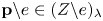 $ {\mathbf {p}} \backslash e \in (Z\backslash e)_\lambda$. Observe that
 $\theta$-stability is not always preserved under this operation. To summarize, for
 $\theta$-stable
 $ {\mathbf {p}} \in Z_\lambda$ and edge
 $e\in Q$ we have the following cases:
(1) Both
 $x_e$ and $x_e^{*}$ are non-zero. We can contract $e$ using $x_e$ or $x_e^{*}$ and obtain a $\theta /e$-stable representation.
(2) Exactly one out of
$x_e$, $x_e^{*}$ is non-zero. Suppose $x_e \neq 0$. We can contract $e$ using $x_e$ or delete $e$. Contraction will always produce a $\theta /e$-stable representation, but deletion sometimes destroys stability.(3) Both
$x_e$ and $x_e^{*}$ are zero. Deleting $e$ produces a $\theta \backslash e$-stable representation.


These observations are the ideas behind notation 4.14 below. Before we get there, we address spanning trees in the Nakajima quiver varieties setting.
Lemma 4.5 Take  $\theta \in {\mathbb {R}}^{Q_0}$: if
 $ {\mathbf {p}} \in {\mathcal {R}}(Q)$ is
 $\theta$-stable then
 $K_ {\mathbf {p}}$ is connected.
Proof. Assume  $K_ {\mathbf {p}}$ is not connected. Choose a connected component and let
 $J \subset Q_0$ be the vertices of this component. Let
 $\delta$ be the indicator function for
 $J \subset Q_0$, then elements
 $(t^{\delta (i)}\cdot 1_i)_{i \in Q_0} \in G_ {\mathbf {v}}$ stabilize
 $ {\mathbf {x}}$ for any
 $t \in {\mathbb {G}}_m$. This gives a positive dimensional stabilizer subgroup and contradicts
 $\theta$-stability. One may also see the lemma by decomposing the corresponding quiver representation into two direct summands and using King stability.
4.2 Stability and trees
In a spanning tree  $T \subset Q$, every edge
 $e \in T$ splits
 $T$ into two connected components; call them
 $T_{t(e)}$ and
 $T_{h(e)}$. If
 $\sum _{i \in T_{t(e)}} \theta _i < \sum _{j \in T_{h(e)}}\theta _j$ we take
 $e$ to be oriented as in
 $Q$. If
 $\sum _{j \in T_{h(e)}} \theta _i < \sum _{i \in T_{t(e)}}\theta _j$ we take
 $e$ to be reverse oriented. We may then view
 $T$ as a subquiver of the double quiver
 ${{\overline {Q}}}$.
This orientation may be equivalently defined in slightly different language. Let  $ {\mathbb {R}}^{Q_1}$ be the vector space of functions
 $Q_1 \rightarrow {\mathbb {R}}$ and, for
 $e \in Q_1$,
 $\chi _e$ be the indicator function of
 $e$. Similarly define
 $\chi _v \in {\mathbb {R}}^{Q_0}$ for
 $v\in Q_0$. The incidence homomorphism
 $\text {inc} \colon {\mathbb {R}}^{Q_1} \rightarrow {\mathbb {R}}^{Q_0}$ is defined by
 $\chi _e \mapsto \chi _{h(e)}-\chi _{t(e)}$. The image of
 $\text {inc}$ is the hyperplane
 $\Theta := \{\theta \in {\mathbb {R}}^{Q_0}:\theta \cdot {\mathbf {v}}=0\} \subset {\mathbb {R}}^{Q_0}$. The inc-images of the edges of a spanning tree of
 $T \subset Q$ define a basis of
 $\Theta$. That is, a spanning tree decomposes the stability space
 $\Theta$ into
 $2^{|Q_0|-1}$ simplicial cones. A generic stability parameter
 $\theta$ lies in precisely one of these cones. The cone to which
 $\theta$ belongs then defines an orientation on our spanning tree
 $T$. The discussion above inspires the following definitions.
Notation 4.6 Fix  $\theta \in {\mathbb {R}}^{Q_0}$ a generic stability parameter and let
 $T$ be a spanning tree of
 $Q$. We will write
 $T^{\theta }$ for the oriented spanning tree of
 ${{\overline {Q}}}$ defined by the
 $\theta$-induced orientation.
Define the weight of  $e\in T^{\theta }$ by
 \[ \theta_{e,T} = \sum_{j\in T_{h(e)}} \theta_j>0. \]
It is not hard to check the identity
 \[ \text{inc}\left(\sum_{e\in T^{\theta}} \theta_{e,T}\; \chi_e\right) = \theta. \]
Lemma 4.7 (Orientation is preserved under contraction) Fix  $\theta \in {\mathbb {R}}^{Q_0}$ a generic stability parameter and let
 $T$ be a spanning tree of
 $Q$. For
 $e \in T^{\theta }$, we have that
 $(T^{\theta })/e \subset \overline {(Q/e)}$ is the
 $\theta /e$-oriented spanning tree of the spanning tree
 $T/e \subset Q/e$. Here we abuse notation and refer to the edge in
 $Q$ and a corresponding edge in
 ${{\overline {Q}}}$ by the same symbol
 $e$. Moreover, we have
 $\theta _{e',T}=(\theta /e)_{e',T/e}$ for each edge
 $e'\in T$ different from
 $e$.
Proof. Straightforward.
Definition 4.8 Take  $ {\mathbf {p}} \in {\mathcal {R}}(Q)$. Let
 ${{\overline {K}}}_ {\mathbf {p}}$ be the double quiver associated to the inversion graph
 $K_ {\mathbf {p}}$ and
 \[ {{\overline{D}}} :=\{e\in {{\overline{Q}}}_1 | x_e \text{ is not an isomorphism}\}. \]
The oriented inversion graph 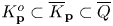 $K_{ {\mathbf {p}}}^{o} \subset {{\overline {K}}}_ {\mathbf {p}} \subset {{\overline {Q}}}$ of
 $ {\mathbf {p}}$ is then
 ${{\overline {Q}}} \backslash {{\overline {D}}}$.
Lemma 4.9 Let  $\theta \in {\mathbb {R}}^{Q_0}$ be a generic stability parameter and take
 $ {\mathbf {p}} \in {\mathcal {R}}(Q)$. The point
 $ {\mathbf {p}}$ is
 $\theta$-stable if and only if there exists a subtree
 $T\subset Q$ such that
 $T^{\theta } \subset K_ {\mathbf {p}}^{o}$.
Proof. Assume  $ {\mathbf {p}}$ is
 $\theta$-stable and that a spanning tree
 $T \subset Q$ for which
 $T^{\theta } \subset K_ {\mathbf {p}}^{o}$ does not exist. Take a tree
 $T \subset K_ {\mathbf {p}}$. We say an edge
 $e \in T^{\theta }$ is faulty if
 $e\notin K_ {\mathbf {p}}^{o}$. Pick a faulty edge
 $e$. Let
 $Q_{t(e)}$ and
 $Q_{h(e)}$ be the subsets of
 $Q_0$ formed by the vertices of
 $T_{t(e)}$ and
 $T_{h(e)}$ respectively. We may assume that there are no arrows
 $a \in {{\overline {Q}}}_1$ from
 $Q_{t(e)}$ to
 $Q_{h(e)}$ whose corresponding linear map
 $x_{a}$ is an isomorphism, otherwise we replace
 $e$ with
 $a$ and get a tree with one less faulty arrow. Setting
 $U_{i} := V_{i}$ for
 $i \in (Q_{t(e)})_0$ and
 $U_{i}:=0$ for
 $i \in (Q_{h(e)})_0$ defines a destabilizing subrepresentation
 $(U_i,\, y_e)$ of
 $ {\mathbf {p}}$.
Now assume  $ {\mathbf {p}}$ is unstable and
 $T$ as above exists. Without loss of generality we can assume that all the arrows outside of
 $T^{\theta }$ are zero. Let
 $ {\mathbf {q}}$ be a destabilizing subrepresentation. If
 $ {\mathbf {q}}$ is decomposable then one of its direct summands is also destabilizing. So we can assume that
 $ {\mathbf {q}}$ is indecomposable, which means that the subgraph
 $K$ of
 $T^{\theta }$ formed by the vertices where
 $ {\mathbf {q}}$ is not zero is connected. The complement
 $T^{\theta }\setminus K$ does not have to be connected, denote its connected components by
 $K_1,\,\ldots ,\,K_m$. We have that there is precisely one edge in
 $T^{\theta }$ from
 $K_i$ to
 $K$ for each
 $i$ and no edges between
 $K_i$ and
 $K_j$ for
 $i\neq j$. The decomposition of
 $T^{\theta }\setminus K$ into connected components corresponds to a decomposition of the quotient
 $ {\mathbf {p}}/ {\mathbf {q}}$ into a direct sum of
 $m$ representations. One of these direct summands is a destabilizing quotient representation, call it
 $ {\mathbf {r}}$. Suppose it is supported on subgraph
 $K_i$. Set
 $ {\mathbf {q}}'=\ker ( {\mathbf {p}}\to {\mathbf {r}})$. We have that
 $ {\mathbf {q}}'$ is supported on
 $K'$, which is formed by the vertices of
 $K$ and
 $K_j$ for
 $j\neq i$. Now
 $K_i$ and
 $K'$ decompose the tree
 $T^{\theta }$ into two parts with a single edge connecting them which goes from
 $K_i$ to
 $K'$. On the other hand, since
 $K_i$ is a destabilizing quotient, we have
 $\sum _{v\in K_i} \theta _v>0>\sum _{v\in K'} \theta _v$, which by the construction of
 $T^{\theta }$ implies that the edge connecting
 $K_i$ and
 $K'$ must be oriented from
 $K'$ to
 $K_i$, a contradiction.
We now want to associate a spanning tree to each  $\theta$-stable point
 $ {\mathbf {p}} \in {\mathcal {R}}(Q)$. The idea here is to pick the ‘biggest’ spanning tree
 $T$ for which
 $T^{\theta } \subset K_ {\mathbf {p}}^{o}$. Such
 $T$ exists by lemma 4.9 since
 $ {\mathbf {p}}$ is
 $\theta$-stable. However, this partial ordering in which this tree is ‘biggest’ is harder to pin down. It is easier to describe it through the smallest edge. We will need the following notation and lemma.
Notation 4.10 Take  $ {\mathbf {p}} \in {\mathcal {R}}(Q)^{\theta }$,
 $e\in Q_1$ and assume
 $ {\mathbf {p}} \backslash e$ is
 $\theta$-unstable; here
 $e$ should be thought of as the smallest edge in some ordering. Every destabilizing subrepresentation of
 $ {\mathbf {p}} \backslash e$ must contain either the head or tail of
 $e$ but not both, otherwise it would destabilize
 $ {\mathbf {p}}$. Furthermore, if one destabilizing representation of
 $ {\mathbf {p}} \backslash e$ contains
 $t(e)$ then they all must: if two destabilizing subrepresentations were to contain both
 $t(e)$ and
 $h(e)$ respectively, then their sum or their intersection must be destabilizing too, which leads to a contradiction. Without loss of generality, we may assume that all destabilizing subrepresentations of
 $ {\mathbf {p}} \backslash e$ contain
 $t(e)$ and do not contain
 $h(e)$. The set of all destabilizing representations, call it
 $ {\mathcal {D}}$, is finite and non-empty. Note that this implies that
 $x_e$ is an isomorphism, otherwise any destabilizing subrepresentation would remain a subrepresentation of
 ${{\overline {Q}}}$. We take
 \[ \beta_e := \text{min}\{\,\theta({\mathbf{q}}) | {\mathbf{q}} \in {\mathcal{D}}\}. \]
We also fix  $\theta ':= \theta - \beta _e \,\text {inc}(\chi _e)$.
Lemma 4.11 Take  $ {\mathbf {p}} \in {\mathcal {R}}(Q)^{\theta }$,
 $e\in Q_1$ and assume
 $ {\mathbf {p}} \backslash e$ is
 $\theta$-unstable. Fix
 $\theta '$ as in notation 4.10. The representation
 $ {\mathbf {p}} \backslash e$ is
 $\theta '$-semistable but not
 $\theta '$-stable. Furthermore,
 $ {\mathbf {p}} \backslash e$ is an extension of two
 $\theta '$-stable representations
 $ {\mathbf {p}}_1$ and
 $ {\mathbf {p}}_2$.
Proof. Take  $\beta _e$ and
 $ {\mathcal {D}}$ as in notation 4.10. Minimality of
 $\beta _e$ gives that elements of
 $ {\mathcal {D}}$ are positive when paired with
 $\theta '$ and so no longer destabilizing. It remains to eliminate the risk of a
 $\theta$-positive subrepresentation of
 $ {\mathbf {p}} \backslash e$ becoming
 $\theta '$-non-positive: if such a subrepresentation was to exist, it would have to contain
 $t(e)$, and its intersection or sum with a
 $\theta$-minimizing element of
 $ {\mathcal {D}}$ would form a
 $\theta$-non-positive subrepresentation of
 $ {\mathbf {p}}$. Strictness of semistability follows since
 $\theta '( {\mathbf {q}})=0$ for a
 $\theta$-minimizing
 $ {\mathbf {q}} \in {\mathcal {D}}$.
For the second statement observe that there is a unique  $\theta$-minimizing subreprestation in
 $ {\mathcal {D}}$: if say
 $\theta ( {\mathbf {q}}_1) =\theta ( {\mathbf {q}}_2)=\beta _e$ for some
 $ {\mathbf {q}}_1,\, {\mathbf {q}}_2 \in {\mathcal {D}}$ then
 $\theta ( {\mathbf {q}}_1\cap {\mathbf {q}}_2) + \theta ( {\mathbf {q}}_1+ {\mathbf {q}}_2)=\theta ( {\mathbf {q}}_1)+\theta ( {\mathbf {q}}_2)$ and minimiality of
 $\beta _e$ implies
 \[ \theta({\mathbf{q}}_1\cap {\mathbf{q}}_2)=\theta({\mathbf{q}}_1+ {\mathbf{q}}_2)=\beta_e, \]
which contradicts genericity of  $\theta$. Here the intersection and sum of
 $ {\mathbf {q}}_1$ and
 $ {\mathbf {q}}_2$ is taken in the ambient representation
 $ {\mathbf {p}}\backslash e$. We take
 $ {\mathbf {p}}_1$ to be this unique
 $\theta$-minimizing element of
 $ {\mathcal {D}}$ and
 $ {\mathbf {p}}_2$ to be the quotient representation
 $( {\mathbf {p}} \backslash e)/ {\mathbf {p}}_1$.
The minimizing property of  $ {\mathbf {p}}_1$ implies it is
 $\theta '$-stable. For stability of
 $ {\mathbf {p}}_2$ observe that any submodule of it corresponds to a submodule of
 $ {\mathbf {p}}$ in such a way that any destabilizing module of
 $ {\mathbf {p}}_2$ gives a
 $\theta$-minimizing module of
 $ {\mathbf {p}}$.
Remark 4.12 For those well versed in GIT language, lemma 4.11 may be alternatively stated as:  $ {\mathbf {p}}$ is
 $S$-equivalent to a
 $\theta '$-polystable representation with two components
 $ {\mathbf {p}}_1$ and
 $ {\mathbf {p}}_2$. One may consult the excellent notes on GIT [Reference Hoskins7] for definitions of
 $S$-equivalence and polystability.
Remark 4.13 It might seem natural to consider the Harder–Narasimhan filtration of  $ {\mathbf {p}} \backslash e$ to get a decomposition into smaller representations. This however does not seem to give the desired results.
As in § 3, we fix an ordering on the edges of  $Q$.
Notation 4.14 Take  $ {\mathbf {p}} \in {\mathcal {R}}(Q)^{\theta }$ and let
 $e$ be the smallest non-loop edge. We define a tree
 $T$ associated to
 $ {\mathbf {p}}$ recursively as follows:
(1) If
$ {\mathbf {p}} \backslash e$ is $\theta$-stable, take $e\notin T$. We then consider $ {\mathbf {p}}\backslash e \in {\mathcal {R}}(Q \backslash e)$.(2) Otherwise take
$e \in T$. We use lemma 4.11 to give us $\theta '$-stable subrepresentations $ {\mathbf {p}}_1$ and $ {\mathbf {p}}_2$; we then consider them on their corresponding subquivers. Applying the algorithm for $ {\mathbf {p}}_1$ and $ {\mathbf {p}}_2$ produces spanning trees in the subquivers, which are then glued together using the edge $e$ to a spanning tree of $Q$.





We stop the algorithm when  $Q$ has one vertex. We will denote the set of all points
 $ {\mathbf {p}} \in {\mathcal {R}}(Q)$ associated to a given spanning tree
 $T \subset Q$ by
 $ {\mathcal {R}}(Q)_T$. Furthermore,
 $Z_{\lambda ,T}^{\theta }$ will be
 $Z_{\lambda } \cap {\mathcal {R}}(Q)_T^{\theta }$.
Lemma 4.15 The algorithm defined in notation 4.14 associates a unique tree  $T$ to every
 $\theta$-stable point
 $ {\mathbf {p}} \in {\mathcal {R}}(Q)$. Furthermore, for
 $ {\mathbf {p}} \in {\mathcal {R}}(Q)_T$ we have that
 $T^{\theta } \subset K_ {\mathbf {p}}^{o}$.
Proof. Existence of  $T$ follows from lemma 4.9 and uniqueness follows from the algorithm in notation 4.14. The last statement follows because in notations used in lemma 4.11
 $x_e$ is an isomorphism and
 $\theta ( {\mathbf {p}}_1)=\beta _e$ is negative, so
 $e$ is oriented the same way as in
 $T^{\theta }$.
The subsets  $ {\mathcal {R}}(Q)_T^{\theta }$ and
 $Z_{\lambda ,T}^{\theta }$ are
 $G_ {\mathbf {v}}$-invariant since
 $\theta$-stability is a
 $G_ {\mathbf {v}}$-invariant property. We will use
 $ {\mathcal {M}}_T \subset {\mathcal {M}}$ to denote the quotient of
 $Z_{\lambda ,T}^{\theta }$ by the
 $G_ {\mathbf {v}}$-action.
For  $e\in K_ {\mathbf {p}}$ a non-loop edge we introduce the notation
 $ {\mathcal {M}}/e$ for the Nakajima quiver variety on the contracted quiver
 $Q/e$ with dimension vector
 $ {\mathbf {v}}= (1,\,\ldots ,\,1)$ and hyperkähler parameters
 $\lambda /e$ and
 $\theta /e$. We use
 $ {\mathcal {M}} \backslash e$ in an analogous fashion.
Theorem 4.16 Let  $T$ be a spanning tree of
 $Q$ and let
 $e$ be the biggest non-loop edge in
 $Q$. If
 $e \in T$ then
 \[ \mathcal{M}_T \simeq (\mathcal{M}/e)_{T/e}. \]
Proof. Without loss of generality we may assume  $T^{\theta }=T$. This in particular implies that
 $x_e$ is an isomorphism. We have a morphism
 $ {\mathcal {M}}_T \rightarrow {\mathcal {M}}/e$ given by
 $ {\mathbf {p}} \mapsto {\mathbf {p}}/e$. In fact the image of this morphism lies in
 $( {\mathcal {M}}/e)_{T/e}$. If we are in case (1) of notation 4.14 on
 $Q$, i.e. the smallest edge
 $e'$ is such that
 $ {\mathbf {p}}\backslash e'$ is stable, lemma 4.3 implies that
 $( {\mathbf {p}}/e)\backslash e'$ is also stable. Therefore, when applying the algorithm to
 $ {\mathbf {p}}\backslash e$ we are in case (1) as well. If we are applying (2),
 $e\in T$ and
 $e$ being the biggest imply that both endpoints of
 $e$ belong to
 $ {\mathbf {p}}_1$ or
 $ {\mathbf {p}}_2$. Hence
 $ {\mathbf {p}}_1/e$ is a destabilizing subrepresentation for
 $( {\mathbf {p}}/e)\backslash e'$, and so the corresponding step of the algorithm for
 $ {\mathbf {p}}/e$ produces the same decomposition of
 $Q_0$, and we can continue by recursion.
On the other hand, a point of  $( {\mathcal {M}}/e)_{T/e}$ lifts to a unique point of
 $ {\mathcal {M}}$ by the following construction. Take
 $ {\mathbf {q}} \in (Z/e)_{\lambda ,T}^{\theta }$; the aim is to provide a lift
 $ {\mathbf {p}} \in Z_{\lambda ,T}^{\theta }$. We start by defining linear maps for every edge in
 ${{\overline {Q}}}$. The linear maps associated to edges not incident to
 $t(e)$ or
 $h(e)$ are clear. For all non-
 $e$ edges incident to
 $t(e)$ and
 $h(e)$, we choose isomorphisms
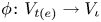 $\phi \colon V_{t(e)} \rightarrow V_\iota$ and
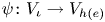 $\psi \colon V_\iota \rightarrow V_{h(e)}$ to unwind their corresponding linear maps and define
 $x_e$ to be
 $\psi \circ \phi$. This choice of
 $\phi$ and
 $\psi$ will come out in the wash when we quotient by the action of
 $G_ {\mathbf {v}}$. The only ambiguity left is the linear map associated to
 $x_e^{*}$. We use the equation corresponding to
 $t(e)$ from (2.2) to read off
 $x_e^{*}$: post-multiplying the equation by
 $x_e^{-1}$ reduces the
 $e$-term to
 $x_e^{*}$. Up to the choice of isomorphisms
 $\phi$ and
 $\psi$, we have a point
 $ {\mathbf {p}} \in Z_\lambda$ and since
 $x_e$ is an isomorphism by construction we have
 $T\subset K_ {\mathbf {p}}^{o}$ which implies
 $ {\mathbf {p}} \in Z_{\lambda }^{\theta }$ by lemma 4.9.
It remains to show that the tree associated to  $ {\mathbf {p}}$ is precisely
 $T$. Suppose this is not the case and denote the corresponding tree by
 $T'\neq T$. Running the algorithm for
 $ {\mathbf {p}}$ produces
 $T'$ and running the algorithm for
 $ {\mathbf {q}}$ produces
 $T/e$. Let us consider the first step where the algorithm for
 $ {\mathbf {p}}$ deviates from the algorithm for
 $ {\mathbf {q}}$ and let
 $e'$ be the smallest edge. We consider the following three possibilities.
Suppose  $e'\notin T'$,
 $e'\in T$. This means that
 $ {\mathbf {p}}\backslash e'$ is stable. By lemma 4.3,
 $( {\mathbf {p}}\backslash e')/e$ is also stable, contradicting
 $e'\in T$. Now suppose
 $e'\in T'$,
 $e'\notin T$. Since
 $e'\notin T$, we have
 $T \subset K^{o}_{ {\mathbf {p}}\backslash e'}$ which implies that
 $ {\mathbf {p}}\backslash e'$ is stable by lemma 4.9. This contradicts the fact that
 $e'\in T'$.
The remaining case is:  $e'\in T$,
 $e'\in T'$ while the decomposition of
 $ {\mathbf {p}}$ into
 $ {\mathbf {p}}_1$ and
 $ {\mathbf {p}}_2$ in (2) of notation 4.14 is different from the corresponding decomposition of
 $ {\mathbf {q}}$ into
 $ {\mathbf {q}}_1$ and
 $ {\mathbf {q}}_2$. This can only happen if
 $e$ connects
 $ {\mathbf {p}}_1$ to
 $ {\mathbf {p}}_2$ so that after contraction of
 $e$,
 $ {\mathbf {p}}_1$ fails to be a subrepresentation of
 $ {\mathbf {q}}$. In this case, we are forced to choose a subrepresentation of
 $ {\mathbf {q}}$ with higher value of
 $\theta$, i.e.
 $\theta ( {\mathbf {p}}_1)<\theta ( {\mathbf {q}}_1)$. We apply the same trick as used in the proof of lemma 4.9: set all maps of
 $ {\mathbf {p}}$ which are not in
 $T$ to zero. Denote the resulting representation by
 $ {\mathbf {p}}'$ and the subrepresentation corresponding to
 $ {\mathbf {p}}_1$ by
 $ {\mathbf {p}}_1'$. Applying our algorithm to
 $ {\mathbf {p}}'$ produces a tree contained in
 $T$, so it must be
 $T$. In particular, the first step of the algorithm produces a subrepresentation which goes to
 $ {\mathbf {q}}_1$ after contraction of
 $e$, so we have
 $\theta ( {\mathbf {q}}_1)\leq \theta ( {\mathbf {p}}_1')=\theta ( {\mathbf {p}}_1)$, a contradiction.
It remains to act by  $G_ {\mathbf {v}}$ to remove the ambiguity of the choice of
 $\phi$ and
 $\psi$ and descend to a morphism
 $( {\mathcal {M}}/e)_{T/e} \rightarrow {\mathcal {M}}_T$. Checking the constructed morphisms are mutual inverses is left to the reader.
Let  $T$ be a spanning tree of
 $Q$ and
 $\theta \in {\mathbb {R}}^{Q_0}$ a generic stability parameter. For every edge
 $e \notin T$, we let
 $C(T,\,e)$ be the unique cycle of the graph obtained by adding
 $e$ to
 $T$. Assume
 $e \notin T$ and let
 $e \neq a \in C(T,\,e)$, the orientation of
 $a \in T^{\theta }$ then defines a direction around
 $C(T,\,e)$ and so an orientation on the edge
 $e$. We call this the
 $a$-induced orientation on e.
Lemma 4.17 Let  $\theta \in {\mathbb {R}}^{Q_0}$ be generic,
 $T$ be a spanning tree of
 $Q,$
 $e$ be the biggest non-loop edge in
 $Q$ and
 $ {\mathbf {p}}=( {\mathbf {x}},\, {\mathbf {x}}^{*}) \in {\mathcal {M}}_T$. Take
 $e \notin T$ and let
 $a$ be the smallest edge in
 $C(T,\,e)$. Assume the
 $a$-induced orientation on
 $e$ is opposite to its orientation as an edge of
 $Q$ then
 $x_e=0,$ otherwise
 $x_e^{*}=0$.
Proof. We may assume  $a$ is the smallest edge of
 $Q$, so
 $a \in T$ implies
 $ {\mathbf {p}} \backslash a$ is
 $\theta$-unstable. We may further assume that
 $t(e)$ is in
 $T_{t(a)}$ while
 $h(e)$ is in
 $T_{h(a)}$. The algorithm in notation 4.14 gives that the representation supported on the vertices of
 $T_{t(a)}$ is a destabilizing subrepresentation of
 $ {\mathbf {p}} \backslash a$, therefore
 $x_e = 0$.
Theorem 4.18 Let  $T$ be a spanning tree of
 $Q$ and
 $e$ be the biggest non-loop edge in
 $Q$. If
 $e \notin T$ then
 \[ \mathcal{M}_T \simeq (\mathcal{M}\backslash e)_T \times {\mathbb{A}}_{{\boldsymbol{k}}}^{1}. \]
Proof. We may now adopt a similar strategy to the proof of theorem 4.16. Take  $ {\mathbf {q}} \in (Z \backslash e)_{\lambda ,T}^{\theta }$; the aim is to provide a lift
 $ {\mathbf {p}} \in Z_{\lambda ,T}^{\theta }$. The linear maps associated to all edges that are not
 $e$ may be read off from
 $ {\mathbf {q}}$. To finish defining the lift, it remains to fix the linear maps
 $x_e$ and
 $x_e^{*}$. Lemma 4.17 allows us to assume that
 $x_e=0$. For the other yet undefined linear map we pick an arbitrary
 $q \in \operatorname {Hom}(V_{h(e)},\, V_{t(e)})$ and set
 $x_e^{*}:=q$. The equations (2.2) in
 $Z_{\lambda ,T}^{\theta }$ then follow directly from those in
 $(Z\backslash e)_{\lambda ,T}^{\theta }$;
 $\theta$-stability follows from lemma 4.9; analysing cases (1) and (2) we deduce that our lift lives in
 $Z_{\lambda ,T}^{\theta }$. This gives a morphism
 \[ (Z \backslash e)_{\lambda,T}^{\theta} \times \operatorname{Hom}(V_{h(e)}, V_{t(e)}) \longrightarrow Z_{\lambda,T}^{\theta}. \]
After acting by  $G_ {\mathbf {v}}$ this descends to a morphism
 $(\mathcal {M} \backslash e)_T \times {\mathbb {A}}_{{\boldsymbol {k}}}^{1} \longrightarrow \mathcal {M}_T.$
Consider  $ {\mathbf {p}}\in {\mathcal {M}}_T$. By lemma 4.17, we can delete
 $e$ and obtain a representation
 $ {\mathbf {q}}$ of
 $Q\backslash e$; this is
 $\theta$-stable by lemma 4.9. The point
 $ {\mathbf {p}}$ is obtained from
 $ {\mathbf {q}}$ by the above lifting construction for a unique value of
 $q \in {\mathbb {A}}^{1}_{{\boldsymbol {k}}}$. If
 $T'$ is the tree associated to
 $ {\mathbf {q}}$, then
 $T=T'$ follows from the first part of the proof.
Corollary 4.19 For  $T\subset Q$ a spanning tree, we have
 $ {\mathcal {M}}_T \simeq {\mathbb {A}}_{{\boldsymbol {k}}}^{b_1(Q)+ \operatorname {ext}(T)}$.
Proof. First we study  $ {\mathcal {M}}_{\lambda ,\theta }(Q,\, {\mathbf {v}})$ when
 $\# Q_0=1$. We have
 $\lambda =0$, so there is an arbitrary choice of linear maps in
 $\operatorname {End}(V_0)$ for every edge of the double quiver
 ${{\overline {Q}}}$, therefore
 $ {\mathcal {M}}= {\mathbb {A}}_{{\boldsymbol {k}}}^{2 (\#Q_1)}$.
We now let  $Q$ be a general quiver. Proposition 3.3 gives that
 $\operatorname {ext}(T) \leq b_1(Q)$ for a spanning tree
 $T \subset Q$. The difference
 $b_1(Q)-\operatorname {ext}(T)$ is precisely the number of times one uses the deletion operator when reducing
 $Q$ to a quiver of one vertex in the recursion computing
 $\operatorname {ext}(T)$.
Theorems 4.16 and 4.18 along with these two observations give that
 \[ {\mathcal{M}}_T \simeq {\mathbb{A}}_{{\boldsymbol{k}}}^{2\operatorname{ext}(T)} \times {\mathbb{A}}_{{\boldsymbol{k}}}^{b_1(Q)- \operatorname{ext}(T)} \simeq {\mathbb{A}}_{{\boldsymbol{k}}}^{b_1(Q)+\operatorname{ext}(T)}. \]
This completes the proof.
Corollary 4.20 The Poincaré polynomial of  $ {\mathcal {M}}$ is given by
 \[ P_{\mathcal{M}}(q) = q^{b_1(Q)} \cdot {\mathbf{T}}_Q(1,q). \]
5. An example: $\widetilde {A}_2$

We go through the calculations in § 4 in an example. The example is relatively simple yet it exhibits most of the phenomena of interest.
Our starting quiver  $Q$ will be that of the affine Dynkin diagram of type
 $\widetilde {A}_2$. We label the vertices and edges of
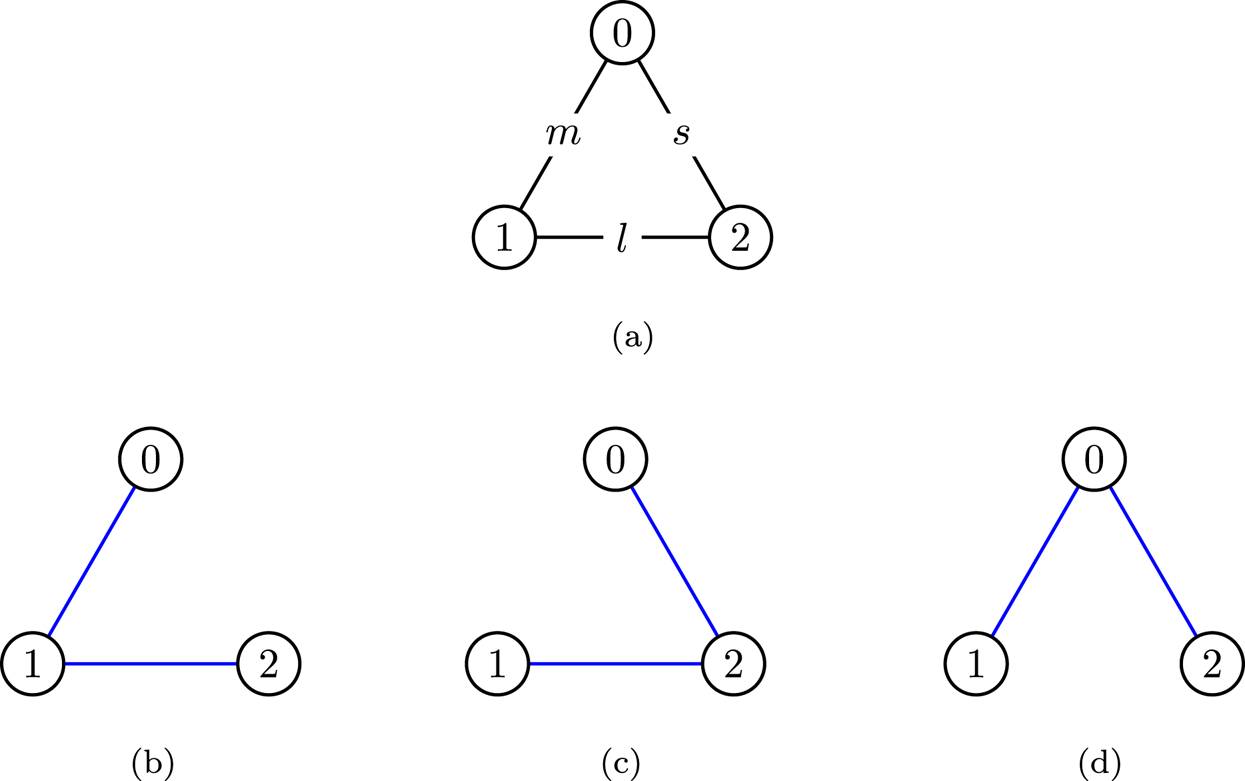
 $Q$ as in figure 1. The figure also contains the three spanning trees of
 $Q$ which are given by forgetting one of the three edges. We pick hyperkähler parameters
 $\lambda =0$ and
 $\theta = (-2,\,1,\,1)$, and we order the edges
 $l>m>s$.
The quiver  $Q$ and its spanning trees. (a) The quiver
 $Q$, (b) Tree
 $T_s$, (c) Tree
 $T_m$, (d) Tree
 $T_l$.

Since our dimension vector  $\mathbf {v}$ is
 $(1,\,\dots ,\,1)$, every representation in
 $ {\mathcal {M}}$ is isomorphic to one where the non-zero vector spaces at the vertices are the vector space
 ${{\boldsymbol {k}}}$. The linear maps at the arrows are then naturally elements of
 $ {\mathbb {A}}^{1}_{{\boldsymbol {k}}}$.
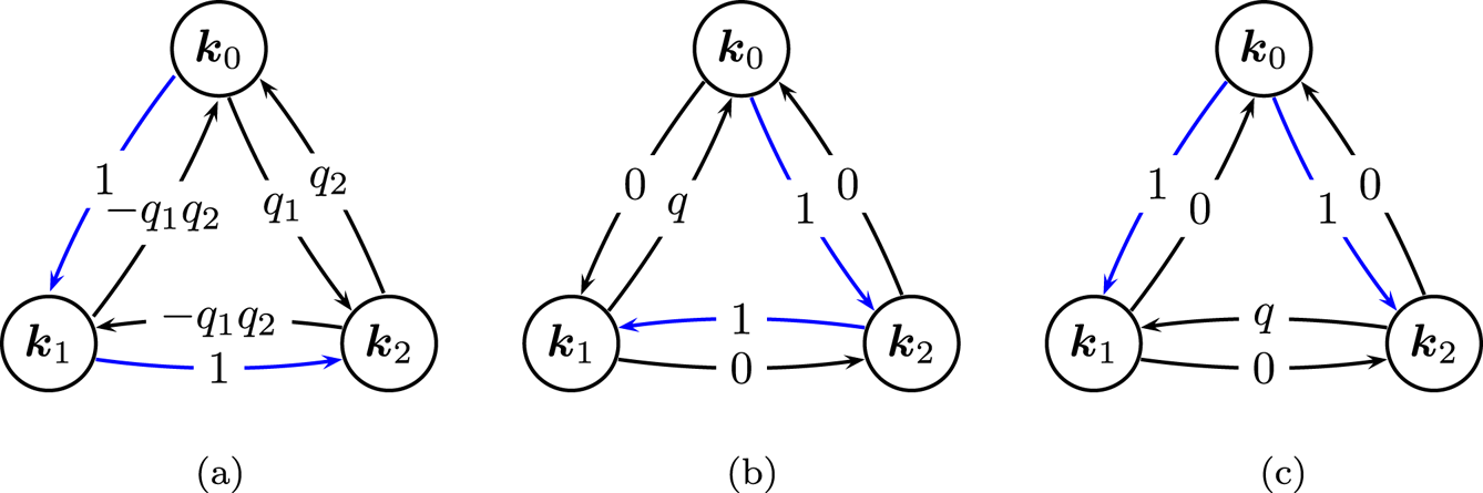
Every point in  $ {\mathcal {M}}$ is equivalent to one of the representations displayed in figure 2. The division into subfigures also indicates the cell
 $ {\mathcal {M}}_{T_i}$ to which the points belong. Arrows in blue indicate the corresponding oriented tree
 ${T_i}^{\theta } \subset {{\overline {Q}}}$. Note that the orientation of the biggest edge
 $l$ (or any edge for that matter) may be different for different spanning trees. The result displayed in figure 2 gives that
 $\# {\mathcal {M}}( {\mathbb {F}}_q)=q^{2}+q+q=q^{2}+2q$.
Cell decomposition of  $ {\mathcal {M}}$, (a)
 $ {\mathcal {M}}_{T_s}$: here
 $(q_1,\,q_2) \in \mathbb {A}_{{\boldsymbol {k}}}^{2}$, (b)
 $ {\mathcal {M}}_{T_m}$: here
 $q \in \mathbb {A}_{{\boldsymbol {k}}}^{1}$, (c)
 $ {\mathcal {M}}_{T_l}$: here
 $q \in \mathbb {A}_{{\boldsymbol {k}}}^{1}$.

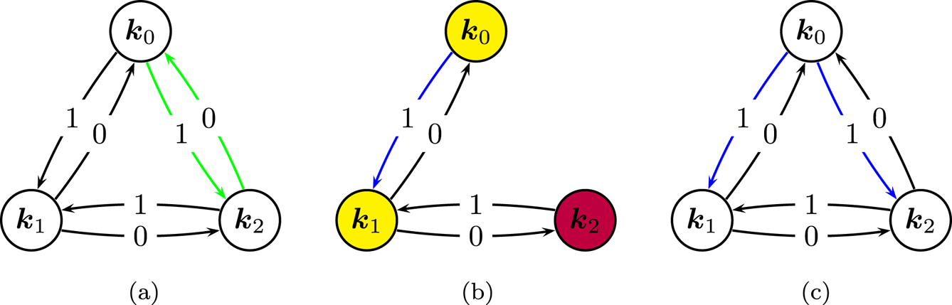
In figure 3 we go through the algorithm in Notation 4.14 for a given point  $ {\mathbf {p}}\in {\mathcal {M}}$. We will indicate the smallest edge using the colour green. The steps in figure 3 give that the tree
 $T_l$ labels the point
 $ {\mathbf {p}}$ given there. Note that
 $T_m^{\theta } \subset K_ {\mathbf {p}}^{o}$. We remark that the algorithm chose
 $T_l$ even though it is lexicographically smaller than
 $T_m$.
Notation 4.14 algorithm. (a) Our point  $ {\mathbf {p}}$. (b) Decomp.
 $\theta '=(-1,\,1,\,0)$. (c) The result.

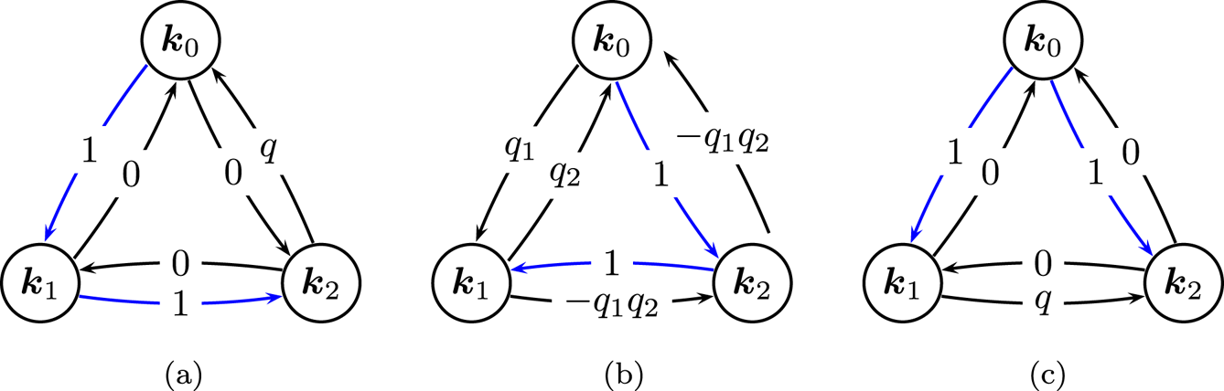
We now change the ordering so that  $s>l>m$ and examine the decomposition of
 $ {\mathcal {M}}$ into cells indexed by spanning trees under this ordering. This cell decomposition is displayed in figure 4.
Cell decomposition of  $ {\mathcal {M}}$: different ordering. (a)
 $ {\mathcal {M}}_{T_s}$: here
 $q \in \mathbb {A}_{{\boldsymbol {k}}}^{1}$, (b)
 $ {\mathcal {M}}_{T_m}$: here
 $(q_1,\,q_2) \in \mathbb {A}_{{\boldsymbol {k}}}^{2}$, (c)
 $ {\mathcal {M}}_{T_l}$: here
 $q \in \mathbb {A}_{{\boldsymbol {k}}}^{1}$.

The decompositions displayed in figures 2 and 4 show that a fixed representation may be labelled by different trees for different orderings. However, they both give decompositions  $ {\mathcal {M}} = {\mathbb {A}}_{{\boldsymbol {k}}}^{2} \sqcup {\mathbb {A}}_{{\boldsymbol {k}}}^{1} \sqcup {\mathbb {A}}_{{\boldsymbol {k}}}^{1}$.
Acknowledgments
The authors are grateful to Layla Sorkatti for helpful discussions. The authors would also like to thank the anonymous referee for their constructive comments. The first author is thankful to the ICTP for supporting them during this project. The second author's work is supported by the projects Y963-N35 and P31705 of the Austrian Science Fund.