





1. Introduction
The specific surface area (SSA) of snow is a critical structural quantity that notably controls the albedo of the snow cover (Grenfell and Warren, Reference Grenfell and Warren1999; Montpetit and others, Reference Montpetit2012) and, therefore, significantly impacts the Earth’s energy budget (Flanner and Zender, Reference Flanner and Zender2006; Zelinka and Hartmann, Reference Zelinka and Hartmann2012). The SSA of snow corresponds to the interfacial area between the ice and air phases per total volume or snow mass. Alongside snow density, the SSA of snow (or direct equivalents such as the optical diameter, for instance) is used in snowpack models to describe the microstructure of the snow layers forming the snowpack (Bartelt and Lehning, Reference Bartelt and Lehning2002; Vionnet and others, Reference Vionnet2012). Such models simulate the physical processes at play in the snowpack and predict its state and physical properties. They are used then in support of avalanche forecasting services (Morin and others, Reference Morin2020), in operational snow-hydrology (Mott and others, Reference Mott, Winstral, Cluzet, Helbig, Magnusson, Mazzotti, Quéno, Schirmer, Webster and Jonas2023) or climate studies (Eckert and others, Reference Eckert, Corona, Giacona, Gaume, Mayer, van Herwijnen, Hagenmuller and Stoffel2024). In a natural snowpack, the SSA of snow is constantly evolving as the snow microstructure continuously changes its spatial arrangement of the ice and air phases, in a process known as snow metamorphism. Besides snow, the properties of metal alloys, polymers and semiconductors similarly depend on the interfacial area between phases. For instance, the tensile strength of Al–Si alloy decreases as the secondary dendritic arm spacing increases (Osório and others, Reference Osório, Goulart, Santos, Neto and Garcia2006; Goulart and others, Reference Goulart, Osório, Spinelli and Garcia2007), which is directly related to the interfacial surface area (Guo and others, Reference Guo, Phillion, Cai, Shuai, Kazantsev, Jing and Lee2017). An accurate understanding and representation of the evolution of the SSA over time is thus of primary importance for studies on snow and of general interest for material sciences. Yet, the SSA evolution in present snowpack models remains poorly estimated (Tuzet and others, Reference Tuzet2017; Calonne and others, Reference Calonne2020), with direct consequences on the ability to accurately model the physical properties of the snow cover.
Under isothermal conditions, mostly occurring in deep snowpacks, the SSA decreases over time in response to curvature variations and the Gibbs–Thomson effect (i.e. the change of the saturated vapor pressure due to surface curvature). This coarsening corresponds to a reduction of excess free energy at the interface between the two phases. The process of coarsening under curvature effects has been extensively studied under the assumption that the microstructure consists of spherical particles with different radii. This corresponds to the seminal coarsening theory first developed by Lifshitz and Slyozov Reference Lifshitz and Slyozov(1961) and Wagner Reference Wagner(1961) (LSW). Overall, the LSW theory predicts that large particles, with lower
interfacial curvature, grow at the expense of smaller particles, with high interfacial curvature. Qualitatively, the theory applies to snow (Löwe and others, Reference Löwe, Spiegel and Schneebeli2011), but specific features stemming from the bi-continuous nature of the material might not be captured. Moreover, truly isothermal conditions only represent a small fraction of the ambient conditions under which snow evolves. Notably, seasonal snowpacks are mostly found under temperature gradient (TG) conditions, due to the temperature difference between the (warm) ground and the (cold) snowpack surface. The work of Snyder and others Reference Snyder, Alkemper, Voorhees and Akaiwa(1999) highlighted that the presence of a small TG affects the coarsening of an idealized microstructure composed of spheres. Consistently, Taillandier and others Reference Taillandier, Domine, Simpson, Sturm and Douglas(2007) experimentally observed that snow coarsening was faster in TG conditions. Moreover, while the SSA of snow usually decreases over time (Taillandier and others, Reference Taillandier, Domine, Simpson, Sturm and Douglas2007; Wang and Baker, Reference Wang and Baker2014; Wiese and Schneebeli, Reference Wiese and Schneebeli2017), a specificity of the snow evolution under TG conditions is the possibility of an SSA increase (Domine and others, Reference Domine, Taillandier, Cabanes, Douglas and Sturm2009; Pinzer and others, Reference Pinzer, Schneebeli and Kaempfer2012; Wang and Baker, Reference Wang and Baker2014). Therefore, theories of SSA evolution in snow must account for the potential presence of a TG as it can significantly impact the coarsening process. In this idea, Flanner and Zender Reference Flanner and Zender(2006) proposed a model of snow coarsening meant for both isothermal and TG conditions. It is, however, based on idealized microstructures composed of non-overlapping spheres rather than actual bi-continuous microstructures. Similarly, Taillandier and others Reference Taillandier, Domine, Simpson, Sturm and Douglas(2007), building on Legagneux and others Reference Legagneux, Taillandier and Domine(2004), proposed a law for coarsening with parameterizations for both isothermal and TG conditions. It assumes a logarithmic decay of the SSA that can be justified in the case of an isothermal system of isolated spheres (Legagneux and others, Reference Legagneux, Taillandier and Domine2004). However, the law underestimates the TG case, and the incorporation of the law into the snowpack model could be a reason for the underestimation of the SSA evolution. Understanding and modeling snow metamorphism under TG, in general, and SSA evolution under TG, in particular, still need to be explored.
The last decades have seen the development of X-ray micro-computed tomography (µCT) in snow sciences, which can measure the microstructure and its evolution over time. This enabled studies simulating the physical processes at play at the pore scale in snow microstructures. Several works proposed to model the dynamical evolution of the microstructure itself (e.g. Flin and Brzoska, Reference Flin and Brzoska2008; Kaempfer and Plapp, Reference Kaempfer and Plapp2009; Krol and Löwe, Reference Krol and Löwe2016; Braun and others, Reference Braun, Fourteau and Löwe2024b). Notably, based on the approach of Drew (Reference Drew1990), Krol and Löwe (Reference Krol and Löwe2018) derived geometrical evolution equations that can be applied to statistically homogeneous microstructures. This rigorous upscaling approach showed that the evolution of the SSA of a microstructure is directly controlled by the average product of the interface velocity and the interfacial mean curvature. In this picture, the accurate determination of the interface velocity plays a key role. This is consistent with, for instance, the study of Park and others Reference Park, Voorhees and Thornton(2015), which pointed out the importance of the interface velocity for the understanding of the complex dynamics of coarsening in bi-continuous structures under curvature effects. In a snow sample, the interface velocity is controlled by the physics responsible for the pore-scale redistribution of water vapor. These mechanisms are currently globally understood and agreed upon and include the diffusive transport of water vapor in the pores of snow (Pinzer and others, Reference Pinzer, Schneebeli and Kaempfer2012; Calonne and others, Reference Calonne, Geindreau and Flin2014) and the deposition/sublimation of the water vapor at the ice–air interface (Libbrecht, Reference Libbrecht2005; Fourteau and others, Reference Fourteau, Domine and Hagenmuller2021b). These can be modeled with the use of numerical simulations (Kaempfer and Plapp, Reference Kaempfer and Plapp2009; Fourteau and others, Reference Fourteau, Domine and Hagenmuller2021a, Yan and others, Reference Yan, Wang and Glicksman2022) and the interface velocity derived in the process.
The use of such numerical simulations, combined with the rigorous SSA equation of Krol and Löwe Reference Krol and Löwe(2018), allowed Braun and others Reference Braun, Fourteau and Löwe(2024b) to simulate the coarsening rate of two samples under TG conditions. The results showed good agreement with experimental data, showcasing the capability of the method to estimate the evolution of the SSA of snow. The simulation work also highlighted the critical role played in the SSA evolution by the condensation coefficient of water vapor onto ice, reflecting how water vapor molecules incorporate into the ice crystal lattice at the ice–air interface (Saito, Reference Saito1996; Libbrecht, Reference Libbrecht2005; Reference Libbrecht2021; Fourteau and others, Reference Fourteau, Domine and Hagenmuller2021b; Bouvet and others, Reference Bouvet, Calonne, Flin and Geindreau2022). However, the dependence of the condensation coefficient on numerous effects such as temperature, supersaturation or crystallographic orientation (Saito, Reference Saito1996; Libbrecht, Reference Libbrecht2005) and fundamental measurement difficulties (Libbrecht, Reference Libbrecht2005) hinder the characterization of the condensation coefficient. Translating these uncertainties of the condensation coefficient on the evolution of snow remains an open question.
In this work, we propose to study the coarsening of artificial microstructure using pore-scale simulations and the SSA evolution equation (Krol and Löwe, Reference Krol and Löwe2018) in order to quantify the drivers of the SSA evolution in snow. The use of artificially generated microstructures enables fine control of the morphology and thus the systematic investigation of a broad range of microstructures. Section 2 recalls the theoretical background used in this article, i.e. the SSA evolution equation and the physics governing the deposition/sublimation of vapor within microstructures. Section 3 then presents the methods employed in our work, specifically the generation of artificial microstructures and the numerical simulations. Finally, Section 4 analyses the physical drivers of the SSA evolution (temperature, TG, condensation coefficient, etc.), proposes a general law to capture the rate of change of SSA in various microstructures under ambient conditions and evaluates the law based on a series of snow µCT images obtained under controlled TG conditions.
2. Theoretical background
As our main motivation comes from understanding snow metamorphism, we adopt the usual framework of snow sciences. We characterize the microstructures in terms of so-called microstructural descriptors (also sometimes referred to as microstructural properties). These microstructural descriptors are a set of scalars meant to characterize the microstructure. They are well-defined at the macroscopic scale (i.e. the scale of a snow layer) and can thus be used in snowpack models to characterize the snow material. They include the ice volume fraction  $\phi_{\mathrm{i}}$ and the SSA (and potentially others). In this article, we use two definitions of the SSA. For a given microstructure, we define the s as the surface of the ice–air interface per total volume (including the ice and air phases), namely
 \begin{equation}s = \frac{S}{V}\end{equation}
with S the surface of the ice–air interface and V the total volume of the microstructure. This definition enables us the direct link to the geometrical evolution of the microstructure via the SSA evolution equation (Krol and Löwe, Reference Krol and Löwe2018).
Historically, snow sciences have rather defined the SSA as the surface of the ice–air interface per total mass of the snow sample (e.g.
Calonne and others, Reference Calonne2020; Martin and Schneebeli, Reference Martin and Schneebeli2023). To enable a direct comparison with previous snow studies, we further define  $\mathrm{SSA_M}$ as the surface of the ice–air interface per snow mass.
 $\mathrm{SSA_M}$ is directly related to s through the product of the ice volume fraction
 $\phi_{\mathrm{i}}$ and the density of ice
 $\rho_\mathrm{i}$:
 \begin{equation}\mathrm{SSA_M} = \frac{s}{\phi_{\mathrm{i}} \, \rho_{\mathrm{i}}}.\end{equation}
The aim of the article is to investigate the evolution of s over time. For this purpose, we rely on the upscaled SSA evolution equation derived by Krol and Löwe Reference Krol and Löwe(2018). It relates the rate of change of s to the velocity field at the ice–air interface within a microstructure. Neglecting the mechanical deformation of the ice matrix, this equation reads as
 \begin{equation}\dot{s} = 2 \,s \, \overline{v_{\textbf{n}}H}\end{equation}
where  $\dot{s}$ is the time derivative of the s,
 $v_\mathrm{\textbf{n}}$ is the normal velocity of the ice–air interface (due to the deposition and sublimation of water vapor), H is the mean curvature of the ice–air interface, and the operator
 $\overline{\bullet}$ stands for the average over the ice–air interface. As classically done with homogenization methods, this equation links the microscopic fields
 $v_\mathrm{\textbf{n}}$ and H (defined at each point of the ice–air interface in the microstructure) and the macroscopic quantity s through the use of surface averaging. We note that Eqn (3) is not limited to snow and applies to any bi-phasic material. The quantity
 $\overline{v_{\textbf{n}}H}$, referred to as the growth rate for the rest of the article, plays a central role. It results from the complex interplay between the movement of water vapor in the microstructure and the local curvature of the microstructure. It corresponds to the relative rate of increase of s, modulo a constant factor 2. A simple geometrical interpretation of the sign of
 $\overline{v_{\textbf{n}}H}$ is displayed in Fig. 1. A negative sign of
 $\overline{v_{\textbf{n}}H}$ indicates that vapor sublimates in convex zones and deposes in concave zones. As illustrated in panel a of Fig. 1, such a sublimation/deposition pattern erodes crests and fills troughs in the microstructure, leading to a flattening of the surface and a decrease of the SSA. Conversely, as seen in panel b of Fig. 1, a positive sign of
 $\overline{v_{\textbf{n}}H}$ indicates that crests and troughs are reinforced, leading to an increase of the SSA.
Geometrical interpretation of the sign of  $\overline{v_{\textbf{n}}H}$ and of the evolution of the SSA, inspired by Drew Reference Drew(1990). (a) Case of a negative sign, where vapor sublimates in convex zones and deposes in concave zones, leading to a decrease of the SSA. (b) Case of a positive sign, where vapor sublimates in concave zones and deposes in convex zones, leading to an increase of the SSA.

While the curvature field H is fully characterized by the microstructure itself, the interface velocity  $v_\mathrm{\textbf{n}}$ depends on the external conditions and physical processes at play. It notably varies with the temperature and the TG to which the sample is subjected. This dependence occurs through the physics governing the movement and deposition/sublimation of water vapor in the microstructure. To model this physics, we follow the typical assumption of a small Péclet number at the pore-scale (Libbrecht, Reference Libbrecht2005) and thus employ the stationary heat and vapor diffusion equations. The water vapor concentration
 $\rho_{\mathrm{v}}$ (expressed in kg m−3) and temperature T (K) fields within a microstructure are thus governed by the following system of equations:
 \begin{equation}\begin{cases}
\nabla^2 T_\mathrm{a} = 0 & \text{in } \Omega_\mathrm{a}\\
\nabla^2 T_\mathrm{i} = 0 & \text{in } \Omega_\mathrm{i}\\
\nabla^2 \rho_{\mathrm{v}} = 0 & \text{in } \Omega_\mathrm{a}\\
T_\mathrm{i} = T_\mathrm{a} & \text{on } \Gamma \\
\kappa_\mathrm{i} \textbf{n} \cdot \nabla T_\mathrm{i} = \kappa_\mathrm{a} \textbf{n} \cdot \nabla T_\mathrm{a} & \text{on } \Gamma \\
\; \nabla \rho_{\mathrm{v}} \cdot \textbf{n} = \frac{\alpha \, v_{\mathrm{kin}}}{D_\mathrm{{v}}}[\rho_{\mathrm{v}} - \rho_{\mathrm{v,s}}(1+d_0 \,H)] & \text{on } \Gamma \\
\end{cases}\end{equation}
where  $\Omega_\mathrm{a}$,
 $\Omega_\mathrm{i}$, Γ and n correspond to the pore space, the ice space, the ice–air interface and the unit normal vector oriented into the pores.
 $T_\mathrm{a}$ and
 $T_\mathrm{i}$ correspond to the temperatures in the air and the ice, respectively.
 $D_\mathrm{v}$ denotes the diffusion coefficient of water vapor in air, κa and κi the thermal conductivities in the air and the ice, respectively, α the condensation coefficient of water vapor onto ice,
 $v_{\mathrm{kin}}$ the so-called kinetic velocity (Saito, Reference Saito1996; Libbrecht, Reference Libbrecht2005; Fourteau and others, Reference Fourteau, Domine and Hagenmuller2021b),
 $\rho_{\mathrm{v,s}}$ the saturated water vapor concentration over a flat surface, d 0 the capillary length and H the local mean curvature. The system of Eqn (4) needs to be complemented with appropriate boundary conditions on the side of the simulated domain, characterizing the temperature and TG to which the snow sample is subjected to.
The capillary length d 0 controls the magnitude of the Gibbs–Thomson effect, i.e. the increase (respectively decrease) of the saturated vapor concentration above convex (respectively concave) ice surfaces. It, therefore, plays a crucial role in isothermal metamorphism, where the redistribution of water vapor at the pore scale is controlled by the curvature effects. It is related to the interfacial energy of ice through  $d_0 = {\gamma \, a_{\mathrm{is}}^3}/(k_{\mathrm{B}} \, T)$, where γ is the interfacial free energy,
 $a_{\mathrm{is}}$ is the mean intermolecular spacing of water molecules in ice and
 $k_{\mathrm{B}}$ is the Boltzmann constant. The product
 $\alpha v_{\mathrm{kin}}$ governs the dynamics at which oversaturated (respectively undersaturated) water vapor is deposited on (respectively sublimated from) an ice surface. The condensation coefficient α corresponds to the probability that a water molecule colliding on the ice crystal surface stays incorporated and the kinetic velocity is given by
 $v_{\mathrm{kin}} = \sqrt{{k_{\mathrm{B}} \, T}/(2\, \pi \,m)}$ with the mass of water molecule m (Saito, Reference Saito1996; Libbrecht, Reference Libbrecht2005; Fourteau and others, Reference Fourteau, Domine and Hagenmuller2021b). Finally, note that for simplicity, the system of Eqn (4) neglects the impact of the water vapor latent heat on the temperature. This assumption results in an overestimation of the vapor fluxes within the microstructure, as the effect of latent heat is to decrease the TG within the air phase. Yet, this overestimation of the vapor fluxes likely remains small (Flanner and Zender, Reference Flanner and Zender2006, Fourteau and others, Reference Fourteau, Domine and Hagenmuller2021a). This is supported by Braun and others Reference Braun, Fourteau and Löwe(2024b), which reports a good agreement between experimental data and simulations neglecting the impact of water latent heat. Under this assumption, the system of equations is thus one way-coupled, the temperature influencing the vapor field, but not the other way around.
The system of Eqn (4) governs the field of water vapor deposition and sublimation, from which the interface velocity  $v_{\textbf{n}}$ can be derived as
 \begin{equation}v_{\textbf{n}} = \frac{D_\mathrm{v} \; \nabla \rho_{\mathrm{v}} \cdot \textbf{n} }{\rho_{\mathrm{i}}} = \frac{\alpha \, v_{\mathrm{kin}}[\rho_{\mathrm{v}} - \rho_{\mathrm{v,s}}(1+d_0 \,H)] }{\rho_{\mathrm{i}}}.\end{equation}
As the interface velocity reflects the movement of the ice–air interface within the microstructure, it has a central meaning for the coarsening process (Park and others, Reference Park, Voorhees and Thornton2015). Again, while Eqns (4)–(5) are given here for snow, they could be used to model other bi-phasic materials. Finally, we note that the obtained interface velocity field, and hence obtained growth rate, corresponds to a ‘snapshot’ value on a given microstructure and that microstructural changes are not simulated in this finite element method (FEM) framework. This work assumption is supported by the separation of time-scale between the rapid heat and vapor processes in the microstructure and the slow evolution of the microstructure.
3. Methods
As the temporal evolution of the SSA is controlled by the growth rate  $\overline{v_{\textbf{n}}H}$, we set up a workflow to derive it from numerical simulations directly performed at the microstructure-scale. This section aims to present the microstructures used in the article and the specificities of the numerical simulations.
3.1. GRF microstructures
3.1.1. Generation of the microstructures
For this study, we explore a range of microstructures, in order to quantify the evolution of the coarsening process for various values of density and SSA. To obtain microstructures spanning a broad range of microstructural characteristics, we rely on artificially generated microstructures using a Gaussian random field (GRF) technique. Microstructures generated from GRFs are, for instance, regularly employed in material sciences to study the electromagnetic and elastic properties of porous structures (Roberts and Garboczi, Reference Roberts and Garboczi2002; Ding and others, Reference Ding, Xu and Tsang2010; Tan and others, Reference Tan, Xiong, Xu and Tsang2016, Soyarslan and others, Reference Soyarslan, Bargmann, Pradas and Weissmüller2018; Blatny and others, Reference Blatny, Löwe, Wang and Gaume2021; Reference Blatny, Löwe and Gaume2023). The generation of GRFs follows the description of Roberts and Teubner Reference Roberts and Teubner(1995), based on a Gaussian spatial correlation function  $G(\boldsymbol{r})$, r being the vector of position. For this study, we use an extended version, which includes a potential spatial anisotropy along the vertical z-axis. Specifically, we construct the correlation function G as a T-periodic Fourier series
 \begin{equation}G(\boldsymbol{r}) = \sum_{l,m,n = -N}^{N}c_{lmn} \; \exp(i {{\boldsymbol{k}_{lmn}}{\boldsymbol{r}}})\end{equation}
where N is the size of the generated sample and  $\boldsymbol{k}_{lmn}= 2\pi/N \, ( l \boldsymbol{\hat{k}}_x + m \boldsymbol{\hat{k}}_y + n \boldsymbol{\hat{k}}_z)$. The real and imaginary parts of complex coefficients
 $c_{lmn} = a_{lmn} + i b_{lmn}$ are taken as Gaussian distributed independent random variables with expected values
 $ \lt a_{lmn} \gt = \lt b_{lmn} \gt = 0$. Their variance is derived from the spectral density
 $\rho(\boldsymbol{k})$ of the correlation function
 \begin{equation} \lt a_{lmn}^2 \gt = \lt b_{lmn}^2 \gt = \frac{1}{2} \rho(\boldsymbol{k}_{lmn}) \left( \frac{2\pi}{3} \right)^3.\end{equation}
Specifically, we assume the correlation function to be Gaussian, i.e.
 \begin{equation}G(\boldsymbol{r}) = \exp(-\frac{r_x^2+r_y^2}{\sigma^2} - \frac{r_z^2}{a^2 \sigma^2})\end{equation}
with σ controlling the standard deviation of the Gaussian correlation function and a an anisotropy ratio along the z-axis. A value of a > 1 corresponds to a vertically elongated microstructure, while a < 1 corresponds to a microstructure with a preferentially horizontal orientation. Note that the inclusion of anisotropy slightly differs from that by Tan and others Reference Tan, Xiong, Xu and Tsang(2016), as an isotropic function with a prefactor based on inclination angle is used there instead. The associated spectral density is
 \begin{equation}\rho(\boldsymbol{k}) = \left( \frac{\sigma}{\sqrt{4 \pi}} \right)^3 \exp(\frac{-\sigma^2}{4}(k_x^2+k_y^2+a^2 k_z^2)).\end{equation}
Once, the coefficients 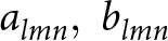 ${a_{lmn},\;b_{lmn}}$ have been randomly generated, the bi-continuous two-phase microstructure
 $\mu(\boldsymbol{r})$ is generated by a level-cut:
 \begin{equation}\mu (\boldsymbol{r}) =
\begin{cases}
\mathrm{ice}, & \text{if } \; G(\boldsymbol{r}) \, \gt \,l\\
\mathrm{pore}, & \text{otherwise}
\end{cases}\end{equation}
where l is a parameter that is to be adjusted to yield the desired ice volume fraction. Following the study by Roberts and Knackstedt Reference Roberts and Knackstedt(1996), the ice volume fraction  $\phi_{\mathrm{i}}$ of the microstructure can be directly related to l as
 \begin{equation}\phi_{\mathrm{i}} = \frac{1}{\sqrt{2 \pi}} \int_{u=l}^\infty \exp \left( -\frac{u^2}{2}\right) \mathrm{d}u.\end{equation}
Therefore, by varying the input parameters l, σ and a, we can produce microstructures with various microstructural properties. The obtained microstructure is defined on a voxel basis, similar to µCT images. We assume a voxel size of 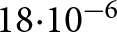 $18{\cdot}10^{-6}$ m for the GRF microstructures, the same voxel size as for the snow sample presented below and visualized in Fig. 3. For the present study, we generated 25 isotropic (a = 1) and 6 anisotropic (a = 0.5 or 2) GRF microstructures with ice volume fraction
 $\phi_{\mathrm{i}}$ ranging from 0.21 to 0.83 (density ranging from 190 to 760 kg m−3) and
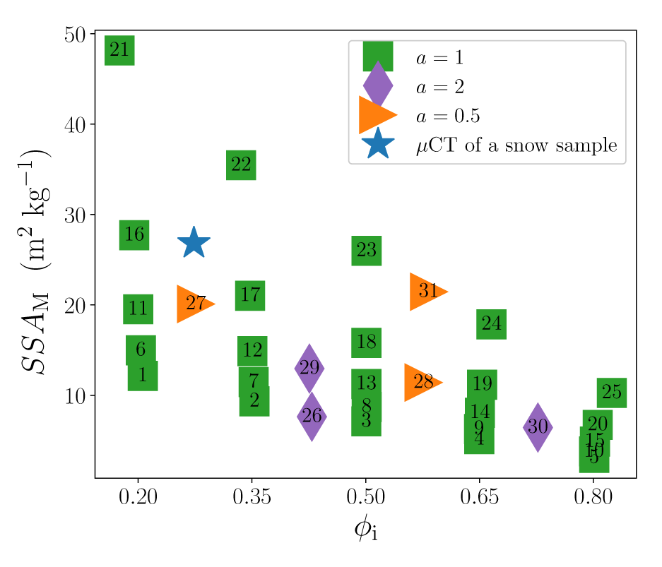
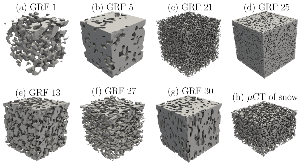
 $\mathrm{SSA_M}$ ranging from 3 to 48 m2 kg−1. The ensemble of 31 generated microstructures is presented in Fig. 2 by their ice volume fraction and SSA, in which each number identifies a GRF microstructure. In the following, we refer to these numbers to specify the GRF microstructures (also called GRFs) and to the ensemble of generated microstructures as the GRF ensemble. The structural variety of the GRF ensemble is illustrated in Fig. 3 by some GRF microstructures.
The ice volume fraction  $\phi_{\mathrm{i}}$ and the SSA
 $\mathrm{SSA_M}$ of the GRF ensemble. Each number corresponds to a GRF microstructure. For a comparison,
 $\phi_{\mathrm{i}}$ and
 $\mathrm{SSA_M}$ of a µCT image of a real snow sample that is presented in Fig. 3 are shown.
Visualization of some GRF microstructures from the GRF ensemble (a-g) and a µCT of a real snow microstructure (h).
3.1.2. Qualitative comparison to real microstructures
While artificial in nature, the generated GRFs are meant to emulate the microstructures of natural material. In particular, the GRFs with low ice volume fraction (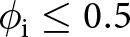 $\phi_{\mathrm{i}}\leq0.5$) will be used to study the SSA evolution of snow and are thus meant to share similarities with it. Due to the nature of GRFs, the generated microstructures present relatively rounded shapes, akin to those found in rounded grains (RG) or melt forms in snow (following the classification of
Fierz and others, Reference Fierz2009). For comparison, an actual fine RG snow microstructure acquired by µCT (from
Pinzer and others, Reference Pinzer, Schneebeli and Kaempfer2012) is displayed in Fig. 3h. This snow microstructure has a ice volume fraction of
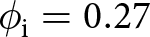 $\phi_{\mathrm{i}} = 0.27$ and
 $\mathrm{SSA_M}$ = 27 m2 kg−1. Typically for snow,
 $\mathrm{SSA_M}$ ranges from around 8–50 m2 kg−1 (Meloche and others, Reference Meloche, Langlois, Rutter, Royer, King, Walker, Marsh and Wilcox2022; Martin and Schneebeli, Reference Martin and Schneebeli2023), a similar range as the one of the GRF generated for this study. Moreover, as seen visually, the morphology of the actual snow microstructure resembles that of the artificial microstructures. Similarly, the GRFs generated with high ice volume fraction (
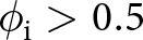 $\phi_{\mathrm{i}} \gt 0.5$) resemble the type of microstructures found in polar firn, with rounded bubbles and pores enclosed in a dense ice matrix (e.g.
Freitag and others, Reference Freitag, Wilhelms and Kipfstuhl2004; Burr and others, Reference Burr, Ballot, Lhuissier, Martinerie, Martin and Philip2018).
3.2. Numerical simulations
The first step of our simulation workflow is designed to provide reliable solutions of heat and mass transport within a microstructure and to derive the deposition/sublimation of water vapor at the ice–air interface (Krol and Löwe, Reference Krol and Löwe2016; Braun and others, Reference Braun, Fourteau and Löwe2024b). For this, the system of Eqn (4) needs to be solved on an accurate representation of the microstructure. We employ the FEM, following the numerical scheme presented in Braun and others Reference Braun, Fourteau and Löwe(2024b). A tetrahedral finite element mesh of the microstructure is generated with the Computational Geometry Algorithms Library (CGAL). In order to properly model the ice–air interface, we first represent the interface as a smooth polyhedral surface and then use the class Polyhedral_mesh_domain_with_features_3 of CGAL, which preserves the surface during tetrahedral meshing. Preserving the ice–air interface is particularly relevant for the computation of the growth rate extracted from that surface. The size of finite elements (tetrahedra and triangles) is controlled by various meshing criteria. The impact of the meshing criteria on the growth rate is assessed below.
The open-source software for multiphysics Elmer FEM (Malinen and Raback, Reference Malinen and Raback2013) is used to solve the stationary heat and vapor diffusion equations on the finite element mesh. The average temperature  $T_{\mathrm{mid}}$ and the macroscopic TG across the microstructure
 $\nabla T$ are specified by imposing the top and bottom temperature of the sample as in Braun and others Reference Braun, Fourteau and Löwe(2024b). In the simulations, the values for
 $v_\mathrm{kin}$ and
 $D_\mathrm{v}$ are taken as constant, while the values for α and d 0 are taken in the ranges
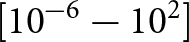 $\left[10^{-6} - 10^2\right]$ and
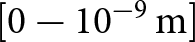 $\left[0 - 10^{-9}\,\mathrm{m}\right]$, respectively. Specifically, the value for the kinetic velocity is set to
 $v_{\mathrm{kin}} =$140 m s−1 (corresponding to
 $T\approx -5^{\circ}\mathrm{C}$) and that of the diffusion coefficient of vapor to
 $D_v = 2\cdot 10^{-5}$ m2 s−1. Note that since
 $v_\mathrm{kin}$ and
 $D_\mathrm{v}$ only appear in the product
 $\frac{\alpha v_\mathrm{kin}}{D_\mathrm{v}}$ in the boundary condition at the ice–air interface (cf. Eqn (4)), the variations of
 $v_\mathrm{kin}$ or
 $D_\mathrm{v}$ are equivalent to variations of α. The assumption that
 $v_\mathrm{kin}$ and
 $D_\mathrm{v}$ are constant therefore does not lead to a loss of generality for the solution of the vapor field. We further assume that the saturated vapor concentration over a flat interface follows the Clausius–Clapeyron condition:
 \begin{equation}\rho_{\mathrm{v,s}}(T) = \frac{m}{k_{\mathrm{B}} \, T} P_0 \exp(\frac{L_\mathrm{fus}}{k_{\mathrm{B}}}(\frac{1}{T_0}-\frac{1}{T}))\end{equation}
with  $T_0=273.15$ K a reference temperature,
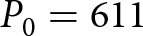 $P_0=611$ Pa the saturated water vapor pressure over ice at T 0 and
 $L_\mathrm{fus}=8.37\cdot10^{-20}$ J the latent heat of sublimation per molecule of water.
The solution of the heat and vapor diffusion simulation yields the field of water vapor deposition and sublimation, from which the interface velocity  $v_{\mathbf{n}}$ can be derived using Eqn (5). The growth rate is then finally obtained, as the product of the
 $v_\mathrm{n}$ and H fields averaged over the ice–air interface in the FEM mesh. For these computations, we employed the Visualization Toolkit (VTK) (Schroeder and others, Reference Schroeder, Martin and Lorensen2006).
3.3. Validation of the numerical workflow
The use of FEM simulations to derive the interface velocity and the growth rate has recently been used in Braun and others Reference Braun, Fourteau and Löwe(2024b). This previous work validated the use of this method to reproduce the growth rate of an idealized spherical microstructure. Furthermore, the method was capable of simulating the SSA evolution of two snow samples under TG conditions. However, to achieve such results it was important that (i) the simulated domain was large enough to be representative of the snow metamorphism process and (ii) that the mesh was refined enough to yield accurate water vapor fields. These two points are discussed below for the current study.
3.3.1. Representative elementary volume
The determination of a representative elementary volume (REV) is essential to derive meaningful results in the study of complex, heterogeneous materials. The REV is defined as the minimum volume of a sample from which a given property becomes independent of the size of the sample (Bear and Bachmat, Reference Bear and Bachmat2012). We define the REV in terms of the growth rate  $\overline{v_{\textbf{n}}H}$. The REV is determined by performing simulations on varying sub-volumes of some GRF structures, with a maximal size-length of 512 voxels (corresponding to 9.2 mm). The dependence of the growth rate on the sample sizes is shown in Fig. 4. It suggests that the REV of the GRF microstructures concerning the growth rate is around 2253 voxels. Thus, for all later presented results, the simulations were carried out on volumes of 2603 voxels, above the REV limit. It’s consistent with the REV sizes determined by Braun and others Reference Braun, Fourteau and Löwe(2024b) for the growth rate of snow.
Dependence of the simulated growth rate on the size of the evaluated microstructure. These computations were performed to determine the REV size by around 2253 voxels.

3.3.2. Spatial discretization error
Besides determining the sensitivity of the growth rate to the microstructure size, the control of the spatial discretization error is evaluated. The use of a very refined mesh is expected to yield the most accurate results but at the expense of a high numerical cost. To ensure the use of a sufficiently refined mesh while keeping a reasonable number of elements, we performed simulations with different degrees of mesh refinement. Specifically, we used the meshing criteria to resize the tetrahedra and surface triangles. As shown in Fig. 5, doubling the number of elements in the finite element mesh impacted the growth rate  $\overline{v_{\textbf{n}}H}$ by about 10
 $\%$. This indicates a rather small dependence on the mesh considering the impact of numerical parameters on the growth rate examined in the next section. The sensitivity analysis emphasizes that the outlined workflow is suitable for investigating the drivers of the SSA evolution.
Impact of the mesh refinement on the simulated growth rate for some extreme cases of GRF microstructures ensemble. Circles indicate the number of elements used in the rest of the article.

3.4. Performed simulations
Obtaining the growth rate  $\overline{v_{\textbf{n}}H}$ is the end goal of our numerical workflow, which starts from a GRF microstructure, performs numerical simulations of heat and water vapor diffusion in the microstructure and finally extracts the growth rate. Using the GRF ensemble allows us to evaluate the impact of the microstructure morphology on the growth rate. Similarly, varying the boundary conditions of the simulations reveals the role of the temperature and TG on the SSA evolution. The workflow also offers the possibility to investigate the role of the pore-scale physics (i.e. the condensation coefficient α or the capillary length d 0) on the growth rate.
We performed simulations with average temperatures  $T_{\mathrm{mid}}$ ranging from 233 to 273 K and with TGs
 $\nabla T$ from 0 to 100 K m−1. To investigate the sensitivity to the pore-scale physics, which remains poorly constrained, we varied the condensation coefficient α between 10−6 and 102 and the capillary length d 0 between 0 and 10−9 m. The upper range of α above unity is taken in order to investigate conditions with highly reactive interfaces. As mentioned above, the values of
 $v_\mathrm{kin}$ and
 $D_\mathrm{v}$ are assumed to be constant. The broad range of numerical simulations resolves various conditions and enables the assessment of dependencies of the growth rate.
4. Results and discussion
4.1. What drives the coarsening of a microstructure?
The goal of this section is to analyze the drivers of the coarsening of microstructures under both isothermal and TG conditions and to analyze the differences of coarsening between microstructures.
Based on the system of Eqn (4) and its boundary conditions, there are four main controls on the growth rate of a microstructure: the average temperature, the TG, the condensation coefficient α (and more generally, the reactivity of the ice–air interface described by the product  $\alpha \, v_\mathrm{kin}$) and the capillary length d 0. Here, we thus investigate the role of these four parameters on the growth rate.
4.1.1. Macroscopic TG
We start with the role of the TG across the microstructure. The magnitude of the TG is expected to control the transition between isothermal metamorphism ( $\nabla T$ close to 0 K m−1) and TG metamorphism (large
 $\nabla T$). For that, we used simulations with TG
 $\nabla T$ varying from 0 to 100 K m−1 and with the other parameters being fixed (
 $T_\mathrm{mid}=265.55$ K,
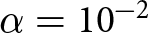 $\alpha=10^{-2}$ and
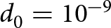 $d_0=10^{-9}$ m as in Braun and others Reference Braun, Fourteau and Löwe(2024b)). Figure 6 displays the impact of the
 $\nabla T$ on the growth rate
 $\overline{v_{\textbf{n}}H}$. For better readability, we do not show the results for all microstructures in the figure, but only for a selection of microstructures, which are representative of the overall GRF ensemble. The graph shows a linear dependence between the growth rate and the TG. Yet, the different microstructures reveal a broad range of behaviors, with some microstructures showing coarsening (i.e.
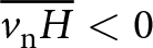 $\overline{v_\mathrm{n} H} \lt 0$) or increase in SSA (
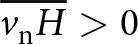 $\overline{v_\mathrm{n} H} \gt 0$). Notably, there is a distinction between microstructures with
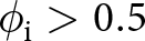 $\phi_{\mathrm{i}} \gt 0.5$ and
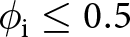 $\phi_{\mathrm{i}}\leq0.5$, the latter being typical for snow. For the microstructures with low ice volume, an increase of
 $\nabla T$ leads to a more pronounced coarsening, while in denser microstructures an increase of
 $\nabla T$ leads to hindered coarsening (or even an increase of the SSA). Finally, a high SSA appears to be linked with a lower influence of the TG, with some high SSA microstructures even showing almost no dependence of the growth rate on
 $\nabla T$.
Dependence of the growth rate  $\overline{v_{\textbf{n}}H}$ on
 $\nabla T$ for low-solid-fraction GRF microstructures in panel (a) and high-solid-fraction microstructures in panel (b). Values obtained from FEM simulation are shown by markers and a linear fit by solid lines. Dotted lines indicate the nonlinear (and almost constant) behavior on a few microstructures. The colors correspond to the SSA of the samples.

The linear dependence of the growth rate on the TG is to be expected, at least with strong TGs when the TG regime is well established. Indeed, in this case, the local influence of temperature on the fluctuation of the saturated water vapor concentration at the ice–air interface overrides the influence due to the local curvature. For the system of Eqn (4), the dominance of local temperature implies that the last equation can be replaced by  $ \textbf{n} \cdot \nabla \rho_{\mathrm{v}} = \frac{\alpha \, v_{\mathrm{kin}}}{D_\mathrm{{v}}}[\rho_{\mathrm{v}} - \rho_{\mathrm{v,s}}(T)]$. Moreover, under the assumption of separation between the microscopic (pore size) and macroscopic (microstructure size) scales, the saturated vapor can be linearized, i.e.
 $\rho_{\mathrm{v,s}}(T) = \rho_{\mathrm{v,s}}(T_{\mathrm{mid}}) + \beta(T_{\mathrm{mid}}) \left( T - T_{\mathrm{mid}} \right)$, with
 $\beta(T)$ the derivative of the saturated vapor with respect to the temperature. Under this condition, the fluctuations of the field
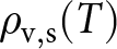 $\rho_{\mathrm{v,s}}(T)$ becomes directly proportional to
 $\nabla T$, since the fluctuations of T are proportional to
 $\nabla T$ (e.g.
Moyne and others, Reference Moyne, Batsale and Degiovanni1988; Calonne and others, Reference Calonne, Geindreau and Flin2014). The field
 $\rho_\mathrm{v,s}$ is then composed of an average value
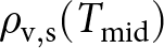 $\rho_\mathrm{v,s}(T_{\mathrm{mid}})$ and a spatially fixed pattern proportional to
 $\nabla T$. In these circumstances, the water vapor deposition/sublimation, and hence the interface velocity
 $v_\mathbf{n}$, becomes directly proportional to the macroscopic TG. Yet, for three microstructures with high SSA, the dependence on
 $\nabla T$ is very small (notably visible as horizontal curves in Fig. 6) and shows a quadratic form (rather than a straight line). This peculiar behavior (in disagreement with linear behavior expected when the TG regime is well established) could be due to interactions between the TG and the curvature influence of the vapor field inside the microstructures. The TG regime on these microstructures could be better established at very high
 $\nabla T$. Apart from these exceptions for the microstructures with high SSA and minor changes in the growth rate, the dependence of the growth rate on the TG seems to be well represented by the linear function. The linear relation could, therefore, be used as the first approximation to estimate the contribution of TG to the growth rate.
4.1.2. Average temperature
A second important control on SSA evolution is the average temperature of the sample. In the system of Eqn (4), the average temperature mainly contributes to the growth rate via the saturated vapor  $\rho_\mathrm{v,s}$ in the Robin boundary condition at the ice–air interface. The specific impact of the average temperature is different depending on whether isothermal or TG metamorphism is at play.
In the isothermal case, the boundary condition at the ice–air interface simply is  $\textbf{n} \cdot \nabla \rho_{\mathrm{v}} = \frac{\alpha \, v_{\mathrm{kin}}}{D_\mathrm{{v}}}[\rho_{\mathrm{v}} - \rho_{\mathrm{v,s}}(T_{\mathrm{mid}})(1+d_0 H)]$. Linearizing
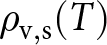 $\rho_{\mathrm{v,s}}(T)$ as in the above discussion on
 $\nabla T$, the field
 $\rho_{\mathrm{v,s}}(T)(1+d_0 H)$ is formed by an average value
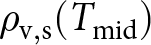 $\rho_{\mathrm{v,s}}(T_{\mathrm{mid}})$ and the spatial pattern
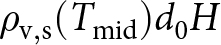 $\rho_{\mathrm{v,s}}(T_{\mathrm{mid}}) d_0 H$. The interface velocity is proportional to these spatial fluctuations. Thus, in the isothermal case, the growth rate inherits the dependence of
 $\rho_\mathrm{v,s}$ on the average temperature
 $T_{\mathrm{mid}}$. Thus, in the isothermal case,
 $v_\mathbf{n}$ and the growth rate
 $\overline{v_{\textbf{n}}H}$ inherit the dependence of
 $\rho_\mathrm{v,s}$ on the average temperature
 $T_{\mathrm{mid}}$. The linear dependence of the growth rate on
 $\rho_\mathrm{v,s}$ is confirmed by isothermal simulations, performed at various average temperatures and everything else left the same. The simulation results are shown for two microstructures in Fig. 7a. In general, the derived linear relation is valid regardless of microstructure.
A similar analysis can be performed for the TG case. Here, the vapor fluxes are driven by fluctuations in the temperature field. As seen in the analysis on  $\nabla T$, the interface velocity
 $v_{\mathbf{n}}$ is proportional to β. Therefore,
 $v_\mathbf{n}$ and the growth rate
 $\overline{v_{\textbf{n}}H}$ depend on the average temperature through β. This is confirmed by TG simulations (
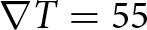 $\nabla T=55$ K m−1) with varied β and everything else left the same. Figure 7b shows that
 $\overline{v_\mathrm{n} H}$ is proportional to β in these TG simulations.
(a) Growth rate  $\overline{v_{\textbf{n}}H}$ against the saturated vapor concentration
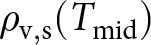 $\rho_{\mathrm{v,s}}(T_{\mathrm{mid}})$ in the isothermal case, for
 $T_\mathrm{mid}$ ranging between 230 and 273 K. (b) Growth rate
 $\overline{v_{\textbf{n}}H}$ against the derivative of saturated vapor concentration β in the TG case.

4.1.3. Surface kinetics and diffusion effects
Other important controls on the water vapor movement in snow, and thus on the SSA evolution, are the surface reactivity, which we describe as  $\alpha \, v_\mathrm{vkin}$ and the diffusivity of water vapor
 $D_\mathrm{v}$. Together, they control the transition between kinetics-limited (KL) and diffusion-limited (DL) growth. Yet, despite its importance for snow physics, the condensation coefficient α remains poorly characterized due to its measurement difficulty. It may well be that our description of surface kinetics is too simplified and that future work needs to investigate the dependence of attachment and detachment kinetics for different crystal surfaces. In our simulations, we chose to investigate a wide range of bulk (spatially constant) condensation coefficients, ranging from 10−6 (typically in the KL regime) to 102 (DL regime). To probe the role of α and the KL to DL transition, we set
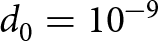 $d_0=10^{-9}$ m,
 $T_{\mathrm{mid}}=265.55$ K and
 $\nabla T = 55\,\mathrm{K\, m^{-1}}$. Simulated
 $\overline{v_\mathrm{n}} H$ is displayed in Fig. 8a as a function of α. For all GRFs, the growth rate
 $\overline{v_\mathrm{n}} H$ appears to vanish for vanishing α. The vanishing α physically corresponds to an inert snow surface, onto which no deposition nor sublimation occurs. In this extreme case, no snow metamorphism happens, and the growth rate is null. In another extreme case, for high α, the growth rate reaches a plateau. Attaining a specific level is consistent with DL growth, under which the diffusion of vapor (i.e.
 $D_\mathrm{v}$) in the pores is the limiting factor, and the reactivity of the interface does not further control the deposition/sublimation of water vapor (Lifshitz and Slyozov, Reference Lifshitz and Slyozov1961). We note that in Fig. 8 this plateau is not visible for some microstructures, either because the curve lies outside the graph (e.g. GRFs 15, 17, 21) or because the plateau appears not be fully reached for a value of α=102 (e.g. GRFs 06 or 12). There is a smooth transition between these cases with clear microstructure differences. Some microstructures (e.g. GRF 12, 17 and 21 in Fig. 8) demonstrate a monotonous transition between the KL and DL regimes. Others (e.g. GRF 05, 15 and 19 in Fig. 8) disclose a non-monotonous transition, with an intermediate regime of SSA-increase between the KL and DL regimes. This non-monotonous behavior appears to be only present in sufficiently dense microstructures. This SSA growth behavior might be related to Mullins–Sekerka instabilities (Mullins and Sekerka, Reference Mullins and Sekerka1964), i.e. tips growing faster than dips in a surrounding vapor field. However, as this phenomenon mainly appears for dense microstructures (
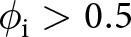 $\phi_{\mathrm{i}} \gt 0.5$), it is likely irrelevant for natural snow.
Impact of the condensation coefficient α on the growth rate  $\overline{v_{\textbf{n}}H}$ for low-solid-fraction GRF microstructures in panel (a) and high-solid-fraction GRF microstructures in panel (b) . Markers correspond to the results from the FEM simulations and dashed lines correspond to fits based on Eqn (13). Note that for some GRF, the DL plateau is out of the y-axis range.

Braun and others Reference Braun, Fourteau and Löwe(2024b) analyzed the idealized case of a sphere growing in a surrounding vapor field and proposed an analytical formula that includes the dependence to α,  $v_\mathrm{kin}$ and
 $D_\mathrm{v}$. It has the same overall shape as the lighter samples of Fig. 8a, i.e. a monotonous decrease of
 $\overline{v_\mathrm{n} H}$ with increasing alpha, with a vanishing growth rate for α = 0 and a plateau for large α. Following the analytical sphere formula of Braun and others Reference Braun, Fourteau and Löwe(2024b), we propose to model the transition from the KL to the DL regimes as
 \begin{equation}\frac{a_0 D_\mathrm{v}}{1+\frac{D_\mathrm{v}}{\alpha \, v_{\mathrm{kin}} \, a_1}}\end{equation}
where a 0 and a 1 are two free parameters (microstructure-dependent). The formula fits the notions of the KL and DL case: it is proportional to α for small α and to the diffusion coefficient  $D_{\mathrm{v}}$ for large α. Moreover, the nondimensional second Damköhler number
 $Da = \alpha \, v_{\mathrm{kin}} a_1 \, /D_{\mathrm{v}}$ arises as the control between the KL (
 $Da \lt \lt 1$) and DL (
 $Da \gt \gt 1$) regimes. The essential role of the second Damköhler number is emphasized in studies that characterize the relative dynamics of the diffusion and surface kinetics processes (e.g.
Bourbatache and others, Reference Bourbatache, Millet and Moyne2020). We note that by design, this formula can only predict a monotonous transition between the KL and DL regimes.
Figure 8a shows the fit of Eqn (13) on a few microstructures and reveals a good agreement between Eqn (13) and the simulations. It is remarkable that the proposed formula (which is monotonous and SSA-increasing by construction) can also be roughly applied to the GRF microstructures with a non-monotonous transition between the KL and DL regimes, if the SSA-increase part is discarded.
4.1.4. Curvature effects
Finally, we focus on the influence of the capillary length d 0, which encodes the sensitivity to curvature fluctuations. The capillary length parameter plays a crucial role in the case of isothermal metamorphism, in which the vapor movements are driven by curvature differences (Krol and Löwe, Reference Krol and Löwe2016). Following the argument advanced for the study of the influence of  $T_{\mathrm{mid}}$ in the isothermal case, the fluctuations of the saturated vapor concentration (driving the interface velocity) are proportional to
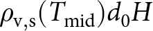 $\rho_\mathrm{v,s}(T_{\mathrm{mid}})d_0 H$, i.e. proportional to the capillary length d 0. Numerical simulations performed under isothermal conditions confirm the proportionality between the growth rate and d 0 in the isothermal case. The isothermal case is well-studied, and we concentrate only on TG simulations for brevity.
The TG metamorphism case is more problematic, as the simple analysis carried out so far is no longer possible. The spatial pattern of saturated vapor is no longer proportional to d 0, as it modifies its shape due to the interaction between the curvature and temperature fluctuations. Hence, to study the influence of d 0 in the TG case, we rely on the numerical simulations (performed with  $T_{\mathrm{mid}}=265.55$ K,
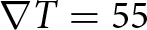 $\nabla T = 55$ K m−1 and
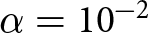 $\alpha = 10^{-2}$). The results of the numerical simulations, displayed in Fig. 9, indicate that the linear dependence to d 0 holds in the TG case. Moreover, all GRFs indicate a trend toward coarsening with increasing d 0. The coarsening trend is in accordance with the capillary length control over the curvature effect’s magnitude. The curvature effect redistributes mass from the areas of high curvature toward low curvatures, which favors the coarsening of the microstructure. Microstructures with high SSA (especially GRFs 21–25) are more sensitive to the influence of curvature effects since they have more curvature fluctuations.
Impact of the capillary length d 0 on the growth rate  $\overline{v_{\textbf{n}}H}$ for low-solid-fraction GRF microstructures in panel (a) and high-solid-fraction GRF microstructures in panel (b).

4.2. An equation for snow coarsening applicable in snowpack models
4.2.1. The general form of growth rate equation
The previous section revealed some specific features of the coarsening process under both isothermal and TG metamorphism, namely, the role of temperature  $T_{\mathrm{mid}}$ on
 $\rho_\mathrm{v,s}$ and β during isothermal and TG conditions, the linear dependence on
 $\nabla T$ and d 0 and the overall shape of the KL to DL transition. Based on those results, we search for a macroscopic formula to model the coarsening process, considering the influence above of
 $T_{\mathrm{mid}}$,
 $\nabla T$, α, etc. This formula is meant to apply directly at the macroscopic level, i.e. it only involves quantities well-defined at the scale of a snow layer. This last point is necessary for use in (macroscopic) snowpack models.
As the equation governing the growth rate, we propose:
 \begin{equation}\overline{v_\mathrm{n} H} = - \frac{\frac{D_\mathrm{v}}{\rho_\mathrm{i}} \, \left( A(\mu) \, \beta \, \nabla T + B(\mu) \, \rho_{\mathrm{v,s}} \, d_0 \right) }{1+\frac{D_\mathrm{v}}{\alpha \, v_{\mathrm{kin}} \, L(\mu)}}\end{equation}
i.e. in terms of SSA
 \begin{equation}\dot{s} = 2 s \overline{v_\mathrm{n} H} = - 2 s \frac{\frac{D_\mathrm{v}}{\rho_\mathrm{i}} \, \left( A(\mu) \, \beta \, \nabla T + B(\mu) \, \rho_{\mathrm{v,s}} \, d_0 \right) }{1+\frac{D_\mathrm{v}}{\alpha \, v_{\mathrm{kin}} \, L(\mu)}}\end{equation}
where A, B and L are free parameters that depend on the microstructure µ. The form of Eqn (14) supposes that the growth rate is the sum of a TG contribution (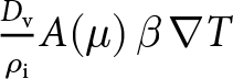 $\frac{D_\mathrm{v}}{\rho_\mathrm{i}} A(\mu) \, \beta \, \nabla T$) and an isothermal contribution (
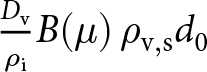 $\frac{D_\mathrm{v}}{\rho_\mathrm{i}} B(\mu) \, \rho_{\mathrm{v,s}} d_0$), and that both are controlled by a similar KL to DL transition (
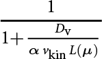 $\frac{1}{1+\frac{D_\mathrm{v}}{\alpha \, v_{\mathrm{kin}} \, L(\mu)}}$).
The equation offers a direct interpretation of the three parameters A, B and L. A (expressed in m−1) encodes the sensitivity of the microstructure toward TG coarsening, B (expressed in m−3) encodes the sensitivity of the microstructure toward isothermal coarsening and L (expressed in m) is a length, controlling the transition from KL to DL coarsening. Based on the interpretation of the Damköhler number  $Da = \alpha \, v_{\mathrm{kin}} \, L/D_\mathrm{v}$ (Bourbatache and others, Reference Bouvet, Calonne, Flin and Geindreau2020), L should scale with the characteristic length at which the water vapor diffusion process occurs. In that sense, A, B and L can be viewed as the material properties that govern the coarsening process, just as thermal conductivity is the material property that governs the heat conduction process. By construction, the proposed governing equation for the growth rate can only predict coarsening (with A, B and L positive) and, therefore, does not capture the increase in SSA observed in dense microstructures at the transition between the KL and DL regimes. Moreover, Eqn (14) directly sums the contribution of the curvature and TG growth rates, neglecting a potential interaction between the two. Under TG conditions, we thus expect our formula to best work in situations where the curvature effects are overridden by the TG, which could be facilitated with microstructures having a low sensitivity to isothermal metamorphism (typically low SSA microstructures) and/or a high sensitivity to TG metamorphism.
We evaluated the ability of Eqn (14) to reproduce the coarsening of low-ice-volume microstructures by comparing them with FEM results. For that, we computed random simulations (varying α, d 0,  $\nabla T$ and T) and adjusted the parameters A, B and L for each microstructure with
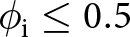 $\phi_{\mathrm{i}} \leq 0.5$. Regarding A, B and L as material properties, we have imposed them to be positive. For each microstructure, we validated the adjustment using a cross-validation technique. The dataset was randomly split into a training set (used to adjust the parameters A, B and L) and a test set containing 50 % of the original dataset. The splitting was repeated 500 times. The performance of the parameterization was assessed by the median of the adjusted coefficient of determination
 $\bar{R}^2$. A unique set of A, B and L computed as the median over splits of found optimal parameters characterizes each microstructure. Figure 10 shows the results of statistical validation for each single microstructure with
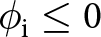 $\phi_{\mathrm{i}} \leq 0$. For each evaluated microstructure, the parameterization performs very well: optimal sets of
 $A(\mu)$,
 $B(\mu)$ and
 $L(\mu)$ were found with
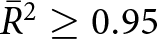 $\bar{R}^2 \geq 0.95$ for all GRF microstructures except for GRF 17 and 18 with
 $\bar{R}^2 =$ 0.83 and 0.86, respectively. The poorer performance of Eqn (14) on GRFs 17 and 18 indicates that its simple form is not able to fully capture the diversity of growth rates predicted by the FEM simulations. As we have a deeper understanding of the dependency of the growth rate on β,
 $\rho_\mathrm{v,s}$, d 0 and
 $\nabla T$, our intuition is that the shortcoming of Eqn (14) likely stems from the assumed α dependency, which might be inadequate. For the evaluated microstructures, ϕi, the structural properties, the range of simulated growth rate and the found values of A, B and L are given in Table 1. Finally, we recall that the growth rate
 $\overline{v_\mathrm{n} H}$ in Fig. 10 can directly be translated as the rate of change of s, using
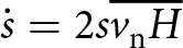 $\dot{s} = 2 s \overline{v_\mathrm{n} H}$.
Agreement between the normalized growth rate  $\overline{v_\textbf{n}\,H}$ obtained from FEM simulations and computed according to the parameter form (Eqn (14)) on single microstructures.

Overview of structural properties ( ${\phi}_{\mathrm{i}}$,
 $\mathrm{SSA_M}$), the number of random simulations (# of sim.), the maximum absolute value of the simulated growth rate
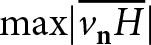 $\max \lvert \overline{v_{\mathbf{n}}H} \rvert$ and the statistical validation results of the derived governing law (median of adjusted coefficient of determination
 $\bar{R}^2$ and the three introduced material properties
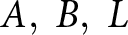 $A, \; B, \; L$) for single GRF microstructures with
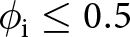 ${\phi}_{\mathrm{i}}\leq 0.5$.

4.2.2. Parameterization of A, B and L for GRF microstructures
The proposed equation (14), which governs the coarsening of snow, introduces three new material properties, namely A, B and L. As stated above, these material properties are direct functions of the microstructure and can be estimated for each microstructure using numerical simulations performed at the pore scale. However, for Eqn (14) to be applicable in snowpack models, the material properties require to be parameterized in terms of microstructural descriptors accessible in models (just like for instance, the snow thermal conductivity is usually parameterized in terms of density for its use in snowpack models). In this section, we thus explore how A, B and L could be parameterized.
We start with L, as it is easily interpretable. As explained above, L is akin to the length over which the diffusion process takes place. It should thus scale roughly with the pore size. Therefore, we propose to express L as a function of  $1/s$. Figure 11 displays a scatter plot of the previously found L values as a function of
 $1/s$. Despite some scatter, it appears that L is linearly related to
 $1/s$ and can be parameterized as
 $a_\mathrm{L} / s$ (
 $a_\mathrm{L}$ being a free parameter to be fitted).
Prediction of A, B and L as functions of the microstructural descriptors. (a) A as a function of  $s/\phi_{\mathrm{i}}$ with a constant fit. (b) B as a function of
 $\sigma_H^{1.5}$ with a linear fit. (c) L as a function of
 $ 1/s$ with a linear fit.

For the parameter B, we exploit that it governs the sensitivity to curvature effects and isothermal metamorphism. It is thus expected to be high in microstructures characterized by sharp variations of the local curvature. Following Krol and Löwe Reference Krol and Löwe2016, we thus search B as a function of the standard deviation of the curvature 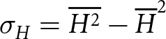 $\sigma_H = \overline{H^2}-\overline{H}^2$. As displayed in Fig. 11, B relates linearly to
 $\sigma_{H}^{1.5}$ quite well. The exponent 1.5 ensures the dimensional consistency between B and σH. Thus, we search B as
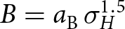 $B = a_\mathrm{B} \, \sigma_H^{1.5}$ with
 $a_\mathrm{B}$ to be fitted. Finally, the parameterization of A revealed itself to be more problematic. In their analysis of snow coarsening under TG, Flanner and Zender Reference Flanner and Zender(2006) proposed that the sensitivity toward TG is related to the fluctuations in inter-granular spacing in snow. While the analysis considers snow as an ensemble of disconnected ice spheres rather than a bi-continuous microstructure, it makes intuitive sense that coarsening under TG conditions is related to the ability of some portions of the microstructure to preferentially attract vapor due to their favored position compared to other portions. Furthermore, Flanner and Zender Reference Flanner and Zender(2006) proposed that the fluctuations in inter-granular spacing scale with the inter-granular spacing itself. In a regular array of spheres, this inter-granular spacing
 $\mathrm{GS}$ is defined as
 \begin{equation}\mathrm{GS} = \left( \frac{4 \pi \phi_{\mathrm{i}}}{s^3 \, \phi_{\mathrm{i}}} \right)^{1/3}-\frac{2 \phi_{\mathrm{i}} }{s}.\end{equation}
However, in the case of the GRF microstructures, we found that using  $\mathrm{GS}$ alone is a poor predictor of A, leading to a large scatter. Motivated by the dimension of A (m−1), we found instead a weak correlation between A and
 $s/\phi_{\mathrm{i}}$, as seen in Fig. 11. No significantly better correlation was found with other simple microstructural descriptors. Thus, in the lack of a better parameterization, we take A as a constant
 $a_\mathrm{A}$ to be adjusted.
Despite the correlations found for the predictions of B and L, some scatter remains, as visible in the three panels of Fig. 11. Hence, the parameterizations proposed in this section are only a preliminary attempt and should be refined to capture better the impact of the microstructure on the coarsening process. Notably, the use of other microstructural descriptors in the parameterization should be considered. As discussed below, it also remains to evaluate how these parameterizations translate for actual snow microstructures.
4.2.3. A parameterized equation for microstructure coarsening
Based on the parameterizations discussed above, we thus propose the following equation to model the growth rate of a microstructure:
 \begin{equation}\overline{v_{\textbf{n}}H} = - \frac{\frac{D_\mathrm{v}}{\rho_\mathrm{i}} \left( a_\mathrm{A} \beta \nabla T + a_\mathrm{B} \sigma_H^{1.5} \rho_{\mathrm{v,s}} d_0 \right) }{1+\frac{D_\mathrm{v}}{\alpha v_{\mathrm{kin}} a_\mathrm{L}/ s}}\end{equation}
i.e. in terms of SSA
 \begin{equation}\dot{s} = 2 \, s \, \overline{v_{\textbf{n}}H} = - 2 \, s \, \frac{\frac{D_\mathrm{v}}{\rho_\mathrm{i}} \left( a_\mathrm{A} \, \beta \, \nabla T + a_\mathrm{B} \, \sigma_H^{1.5} \, \rho_{\mathrm{v,s}} \, d_0 \right) }{1+\frac{D_\mathrm{v}}{\alpha \, v_{\mathrm{kin}} \, a_\mathrm{L}/ s}}\end{equation}
where  $a_\mathrm{A}$,
 $a_\mathrm{B}$ and
 $a_\mathrm{L}$ are three free parameters to be adjusted. We stress that these three parameters are meant to apply for all the GRF microstructures with
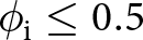 $\phi_{\mathrm{i}}\leq 0.5$. To adjust these parameters and assess the ability of Eqn (17) to predict the growth rate of a range of microstructures, we employ the same cross-validation technique as used above. The resulting values are
 $a_A=134.8$ m−1,
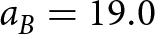 $a_B=19.0$ and
 $a_L=1.13\times10^{-2}$ with a median
 $\bar{R}^2$ of 0.95 and
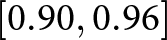 $[0.90, 0.96]$ as the 95 % confidence interval. The results are visualized for the median of free parameters in Fig. 12. As seen in the figure, the scatter is more marked than in Fig. 10. The reason for this is that the reduction of the total number of free parameters (from three per microstructure to only three in total), which results in a degradation of the prediction of the material properties A, B and L. This problem is especially marked for A that varies substantially for different microstructures and that encodes the critical dependence to TG metamorphism. Nonetheless, we have obtained a governing law for the growth rate with only three free parameters that reasonably reproduces the simulated growth rate for various conditions (
 $T_{\mathrm{mid}}$,
 $\nabla T$, α, etc.) and microstructures.
Evaluation of the growth rate  $\overline{v_{\textbf{n}} \, H}$ obtained from Eqn (17) against the FEM simulations on multiple microstructures.

4.3. A first application to snow
Here, we briefly evaluate the ability of the proposed law and parameterization to model the coarsening of actual snow samples. For this, we rely on the experimental data obtained by Pinzer and others Reference Pinzer, Schneebeli and Kaempfer(2012) under controlled TG conditions. The experimental data consist of a time series of µCT images, regularly performed during a  $\sim400$ h long experiment under a TG of 47 K m−1 and an average temperature of
 $-8.1^\circ$C. The experimental growth rate
 $\overline{v_{\textbf{n}}H}$ at the
 $i\mathrm{th}$ time step can be derived as:
 \begin{equation}\overline{v_{\textbf{n}}H} = \frac{\dot{s}}{2 \,s} \simeq \frac{s^{i+1}-s^{i}}{2\, s^{i}\, \Delta t}\end{equation}
where  $\Delta t$ is the time step between two consecutive images.
Moreover, the µCT images provide the necessary microstructural descriptors to apply our proposed growth rate equation with the GRF-based parameterization of A, B and L. For the value of α in the growth rate equation, we follow the work of Braun and others Reference Braun, Fourteau and Löwe(2024b) that found a shift from 10−1 to 10−1.5 around the middle of the experiment. This decrease of the α under TG conditions has been interpreted as a result of the development of facets. The capillary length is taken as 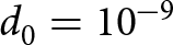 $d_0=10^{-9}$ m (Kaempfer and Plapp, Reference Kaempfer and Plapp2009).
A comparison between the experimental and modeled growth rates is displayed in panel a of Fig. 13. The translation of the growth rates in terms of an SSA time series is displayed alongside in panel b. We note that in the case of the SSA time series, errors on growth rate accumulate over time, potentially leading to a large error at the end of the time series. The transition in α is visible as a sharp drop of the growth rate around the 160 h, both in the modeled and experimental values. The direct application of the growth rate equation with the GRF-based parameterization yields a very good agreement with the experiment in the second part of the time series but clearly underestimates the coarsening in the first part. Our interpretation is that this likely comes from an underestimation of A, the TG sensitivity, from the GRF-based parameterization in the first portion of the experiment that might not be suitable for actual snow. Thus, we assess whether another parameterization of A, B and L could yield a better agreement with the experimental data. For this, we kept the assumed dependence of A, B and L on the microstructural descriptors but re-adjusted the coefficients aA, aB and aL of Eqn (17) on the experimental data. After adjustment, we obtained the optimal values 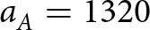 $a_A=1320$ m−1,
 $a_B=1.52\times10^{-2}$ and
 $a_L=1.09\times10^{-2}$. This second parameterization notably yields higher TG sensitivities (A) and smaller length scales governing the KL to DL transition (L). As displayed in panel a of Fig. 13, this results in a better agreement of the growth rates over the whole experimental time series, with notably a faster coarsening in the first part (due to higher A values) and a sharper effect of the α transition (due to smaller L values). In this case, growth rate errors do not accumulate over time, leading to a good prediction of the SSA over the whole time series, as seen in panel b of Fig. 13. These results suggest that when properly parameterized, the growth rate equations proposed in this article can be accurately applied to snow.
Evaluation of the proposed parameterization against experimental observations of snow metamorphism. (a) Comparison between observed growth rates (black) and predicted growth rates using Eqn (17) (blue and orange). (b) Comparison between observed SSA values (black) and the predicted SSA time series integrating Eqn (18) over time (blue and orange).

4.4. Relations to the LSW theory and previous works
Based on the theory of Lifshitz, Slyozov and Wagner (Lifshitz and Slyozov, Reference Lifshitz and Slyozov1961; Wagner, Reference Wagner1961), Legagneux and others Reference Legagneux, Taillandier and Domine(2004) showed that the isothermal SSA evolution of an ensemble of dispersed spheres could be modeled as
 \begin{equation}s(t) = s_0 \left( \frac{\tau}{t+\tau} \right)^{1/n}\end{equation}
with s 0 the initial SSA, τ a characteristic time which is a function of the initial SSA and the physics at play and n an exponent equal to 3 in the DL case and 2 in the KL case. While the formula was derived assuming an ensemble sphere, it has been successfully applied to snow. One can thus wonder how the framework proposed in this article relates to that of Lifshitz and Slyozov (Reference Lifshitz and Slyozov1961), Wagner (Reference Wagner1961) and Legagneux and others Reference Legagneux, Taillandier and Domine(2004), and if they can be reconciled.
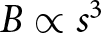
First, we recall that we have assumed above that B could be assumed as proportional to  $\sigma_H^{1.5}$. We have chosen σH as the predictor, as isothermal metamorphism is driven by curvature fluctuations. However, curvature fluctuations are also closely related to the SSA. Indeed, dimensional analysis suggests that σH scales with s 2. This is confirmed by our GRF ensemble, which reveals a linear relation between σH and
 $s^2/\phi_{\mathrm{i}}^2$ (not shown). Therefore, a potential parameterization could also be of the form
 $B \propto s^{3}$.
We now analyze the DL case (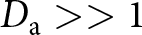 $D_\mathrm{a} \gt \gt 1$). Here, Eqn (15) simplifies to
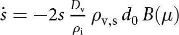 $\dot{s} = - 2 s\, \frac{D_\mathrm{v}}{\rho_\mathrm{i}}\, \rho_\mathrm{v,s}\, d_0\, B(\mu)$. Taking
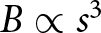 $B \propto s^{3}$, we obtain that
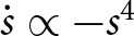 $\dot{s} \propto - s^{4}$. The solution of such differential equation has the form
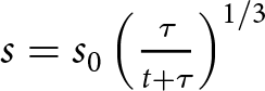 $s = s_0 \left( \frac{\tau}{t+\tau} \right)^{1/3}$. This directly corresponds to the form proposed by Legagneux and others Reference Legagneux, Taillandier and Domine(2004). Similarly, in the KL case (
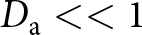 $D_\mathrm{a} \lt \lt 1$), Eqn (15) simplifies to
 $\dot{s} = - 2 s\, \frac{\rho_\mathrm{v,s}}{\rho_\mathrm{i}}\, d_0\, \alpha\, v_\mathrm{kin}\, L(\mu) B(\mu)$. With
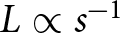 $L \propto s^{-1}$, we have that
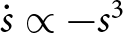 $\dot{s} \propto -s ^{3}$. The solution of this differential equation is
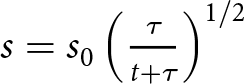 $s = s_0 \left( \frac{\tau}{t+\tau} \right)^{1/2}$. Again, this matches the result of Legagneux and others Reference Legagneux, Taillandier and Domine(2004) for the DL case.
4.5. Current limitations and future work
We expect Eqn (14) to apply for a large range of microstructures (under the restriction that 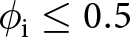 $\phi_{\mathrm{i}}\leq0.5$), as it is informed by the general physics governing deposition and sublimation at the pore-scale. Yet, the parameterization of the material properties A, B and L revealed itself to be more problematic. The difficulty of finding an accurate parameterization for many microstructures results in the spread of Fig. 12.
This is especially due to the difficult parameterization of A, which cannot easily be related to descriptors of the microstructure. Further work should, therefore, be dedicated to investigating its microstructural drivers, i.e. why different microstructures coarsen differently under TG conditions, in an effort to derive a more accurate parameterization. The simplified description of surface kinetics via a spatially and temporally constant factor α can play a role here.
Moreover, the parameterization proposed here for B involves the quantity  $\overline{H^2}$. While this is a well-defined macroscopic quantity, it is usually not included in snowpack modeling. Indeed, models are usually restricted to the ice volume fraction (given by density) and the surface specific area (grain size or optical diameter) in terms of objective descriptors of the microstructure. The use of quantities such as
 $\overline{H^2}$ would thus require to introduce its governing equation, in order to properly close the system of equations. Fortunately, an upscaled equation for
 $\overline{H^2}$ is provided in Krol and Löwe Reference Krol and Löwe(2018). As with the upscaled SSA equation, it involves the interface velocity and the local curvatures, averaged over the ice–air interface of the sample. Translating this equation in terms of macroscopic quantities (density, SSA, etc.) would require a similar treatment as done in this article for the upscaled SSA equation.
In order to avoid the use of  $\overline{H^2}$, we note that it could be possible to rather use a parameterization in terms of s and
 $\phi_{\mathrm{i}}$. While we obtain reasonable results using
 $s/\phi_{\mathrm{i}}$ as a predictor for B, we think that this was helped by the fact that the GRF microstructures share a similar morphology (i.e. the ‘grains’ all resemble RG in the snow classification). The different microstructures can thus be seen as spatially scaled versions of one another: a fine microstructure with a large SSA corresponds to a larger microstructure that would have been spatially shrunk. In this condition, a direct relation between
 $s^2/\phi_{\mathrm{i}}^2$ and
 $\overline{H^2}$ can be expected. However, we do not know if such a relation would hold in the case of microstructures with different morphologies (i.e. different snow types).
Following this last point, a limitation of the work presented here is that, while the use of GRF allows us to precisely control the porosity and SSA of the microstructures, it does not have the variability of natural snow in terms of morphologies. Further work should be dedicated to extend this study to actual snow samples, measured under µCT and to investigate the quantitative differences between morphologies (i.e. facetted crystals, depth hoar, precipitation particles, etc., Fierz and others, Reference Fierz2009) during coarsening under both isothermal and TG conditions.
Finally, we recall that our study did not consider the role of mechanical deformation on the SSA evolution. One reason for this is that the mechanism(s) driving the plastic deformation of snow at the pore-scale remains unknown (Fourteau and others, Reference Fourteau, Freitag, Malinen and Löwe2024) and therefore cannot be implemented in our FEM simulations. Yet, we expect that neglecting the ice matrix deformation is not a strongly limiting assumption of this work. Indeed, while the theoretical equation (15) of Krol and Löwe Reference Krol and Löwe(2018) indicates that the deformation of the ice matrix can have an influence on the SSA, the experimental study of Schleef and Loewe Reference Schleef and Loewe2013 did not observe any impact of the densification on the SSA of light snow samples. The use of pore-scale simulations could be a tool to investigate the relative contribution and interactions of metamorphism and deformation on the SSA evolution, but this will first require an understanding of the mechanism(s) driving the deformation of the ice matrix.
5. Conclusions
In this work, we combined the pore-scale physics governing the deposition and sublimation of water vapor and the upscaled geometrical equation of Krol and Löwe Reference Krol and Löwe(2018) to quantify the rate of change of SSA in various microstructures. For that, we set up the FEM simulations of the water vapor in snow and its deposition/sublimation at the ice–air interface, from which the rate of change of SSA can be assessed. The simulations were performed on artificially generated microstructures, which allows us to precisely control the ice volume fraction and SSA of the microstructures. Despite being artificially generated, these microstructures resemble typical RG of snow at low density and polar firn at higher densities. By working directly with bi-continuous matrices of ice and air, this study does not need to consider snow as an ensemble of spheres, offering a more realistic view of the material.
The simulation revealed a contrasted behavior between low density (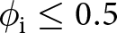 $\phi_{\mathrm{i}}\leq0.5$) and high density (
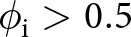 $\phi_{\mathrm{i}} \gt 0.5$) microstructures that we interpret as a difference between convex and concave microstructures. In some conditions, the simulations revealed the possibility of SSA increase, likely related to Mullins–Sekerka interface instabilities.
Based on simple physical arguments, we derive a law governing the coarsening of the microstructures with 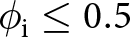 $\phi_{\mathrm{i}}\leq0.5$. This law is meant to be applied under various ambient conditions, isothermal or under a TG. The law explicitly takes into account the influence of the physical parameters controlling the pore-scale processes, namely the diffusion coefficient of vapor in air, the kinetics of surface deposition/sublimation (i.e. the condensation coefficient of water vapor onto ice and the so-called kinetics velocity) and the capillary length. This formula introduces three material properties that fully characterize the coarsening of the microstructures. These material properties directly and solely depend on the microstructure. These coefficients correspond to the sensitivity of the microstructures to coarsening under TG conditions, the sensitivity of the microstructure to coarsening under isothermal conditions and the length scale controlling the transition from KL to DL regimes.
The ability of the proposed formula to capture the coarsening of various microstructures has been verified using the pore-scale FEM simulations (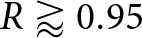 $R \gt rapprox0.95$). Using these simulations, we then investigate the relation between the three new material properties and the microstructure, with the goal of deriving a parameterization applicable in snowpack models. We were able to derive parameterizations for the sensitivity of the microstructure to coarsening under isothermal conditions and the KL to DL length scale, based on the SSA and the second moment of the curvature distribution. However, the parameterization of the sensitivity of the microstructure to coarsening under TG conditions remains evasive, as no clear link with a simple descriptor of the microstructure was observed. Nonetheless, once parameterized in terms of microstructural descriptors, we were able to reasonably predict the coarsening rate of various snow-like microstructures (R ≈ 0.95). Finally, we evaluated the ability of the proposed law to predict experimental snow coarsening data. Direct application of the GRF-based parameterization resulted in an underestimation of the growth rate, but results could be significantly improved by adjusting the TG sensitivity and length scale parameterization.
We believe the approach in this article benefits our comprehension of snow coarsening and its representation in models. Setting a physically based governing law reduces the complexity of the coarsening process to only three material properties that can be estimated from numerical simulations and/or controlled experiments and are directly interpretable. A similar approach could also be used to derive the equation governing the evolution of the curvature and its moment, should it be necessary to close the system of equations describing the evolution of the snow material over time.
Data availability
We published simulation parameters and outputs for this study on the data portal EnviDat, https://doi.org/10.16904/envidat.569 (Braun and others, Reference Braun, Fourteau, Frei, Lehning and Löwe2024a).
Acknowledgements
We thank Marie Dumont for the helpful discussions on the state of the art of SSA modeling and for her valuable inputs on the parameterization proposed in this work.
Author contributions
The research was designed by HL. The program used for GRF generation was developed by SF with supervision of HL. The numerical simulations were performed by AB. The interpretation of the results was performed by AB and KF with the help of ML. The manuscript was written by AB with feedbacks from all co-authors.
Financial support
This research was supported by the Swiss National Science Foundation (SNSF; grant no. 200020_178831). Kévin Fourteau’s position is funded by the European Research Council (ERC) under the European Union’s Horizon 2020 research and innovation program (IVORI; grant no. 949516).
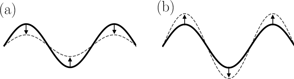

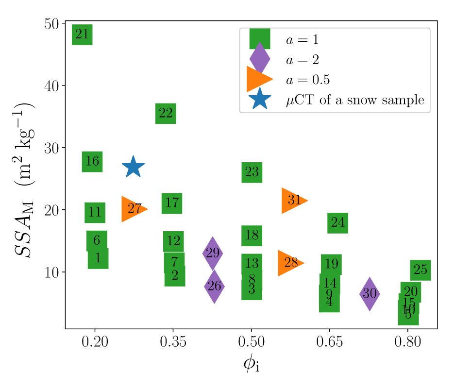


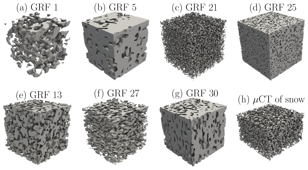
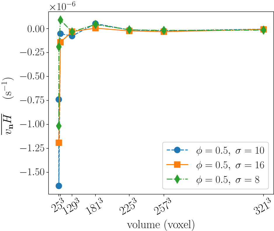
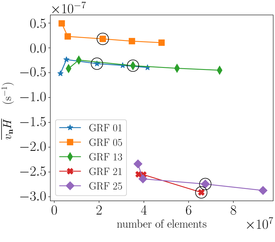
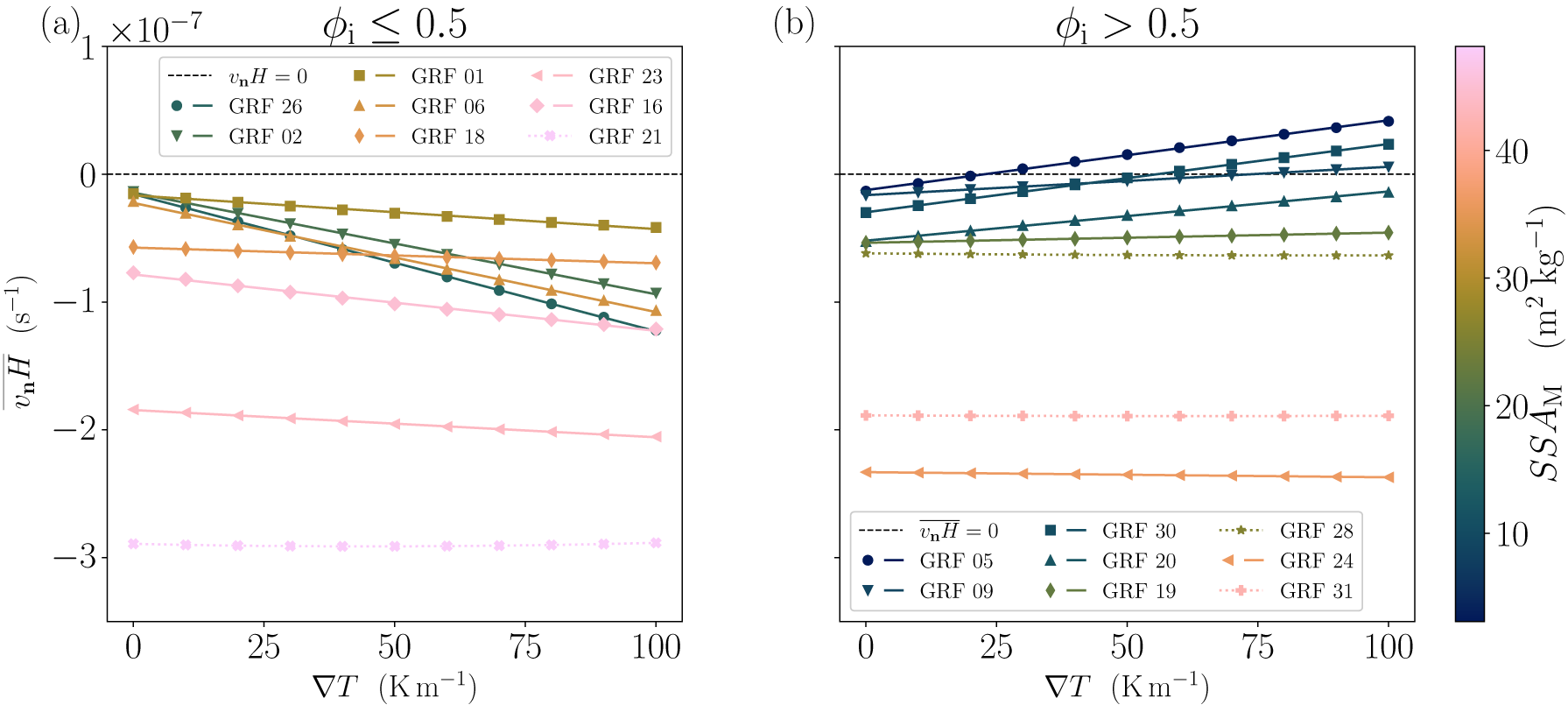


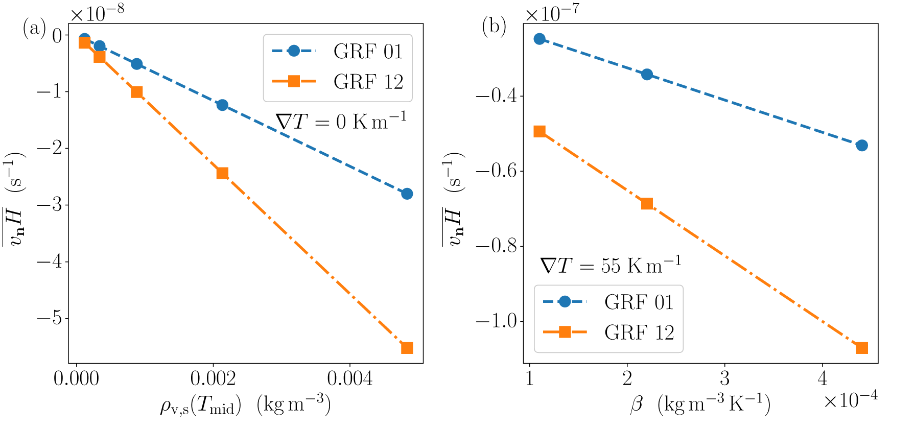


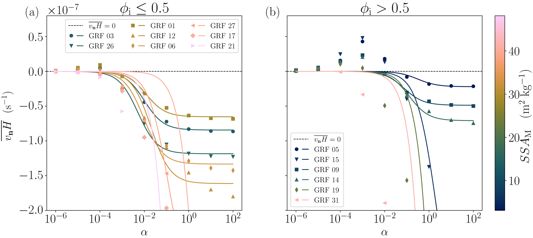

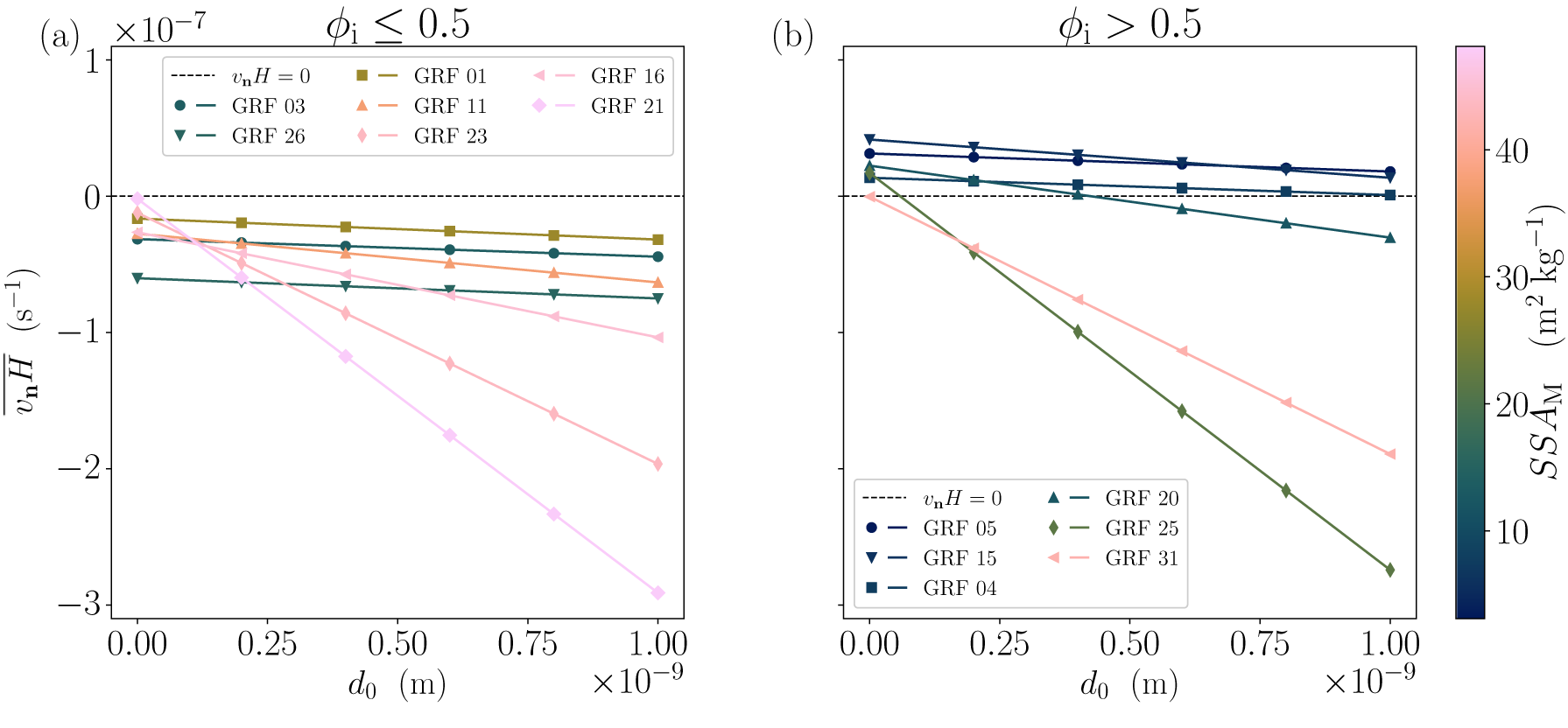

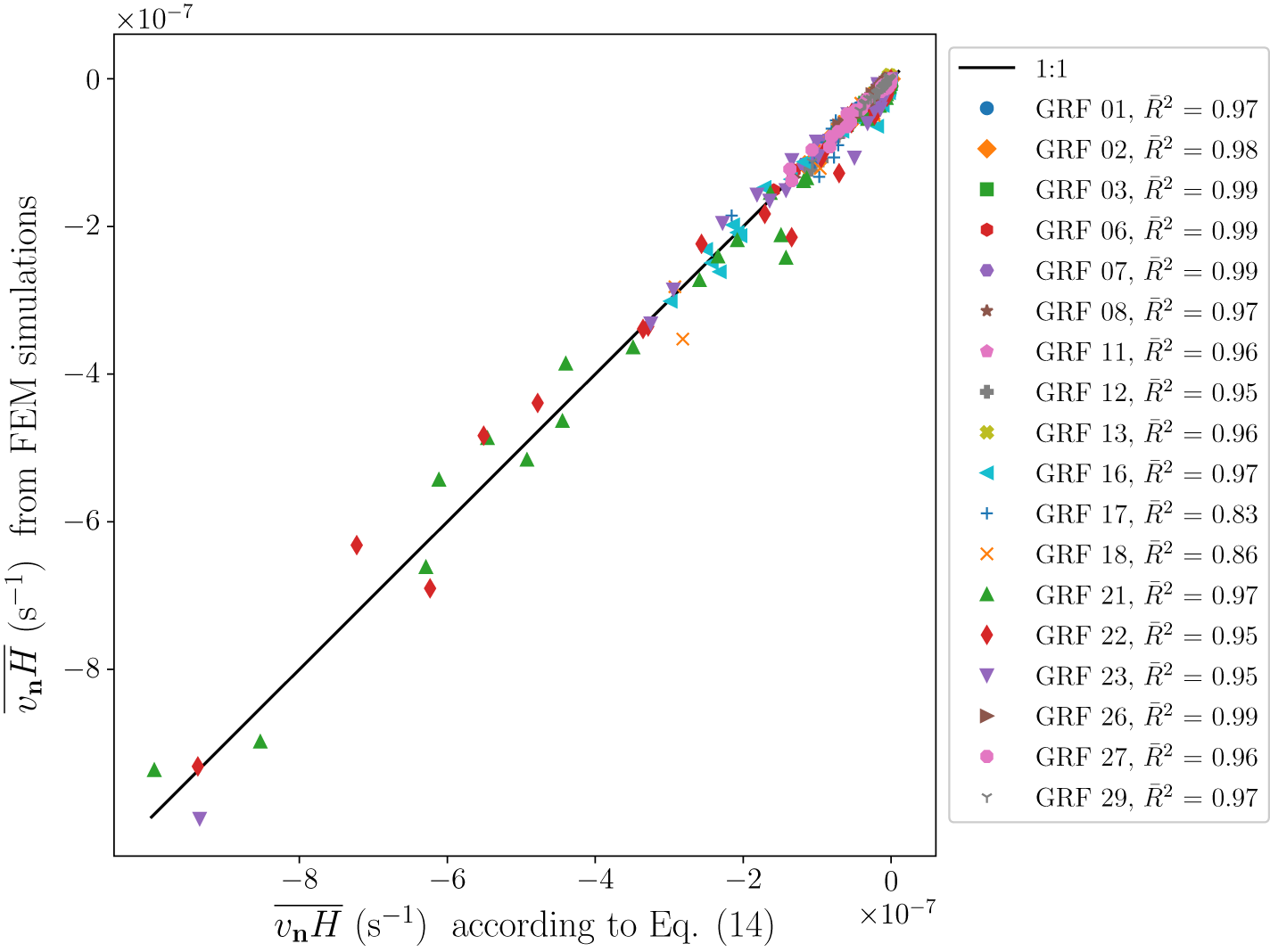

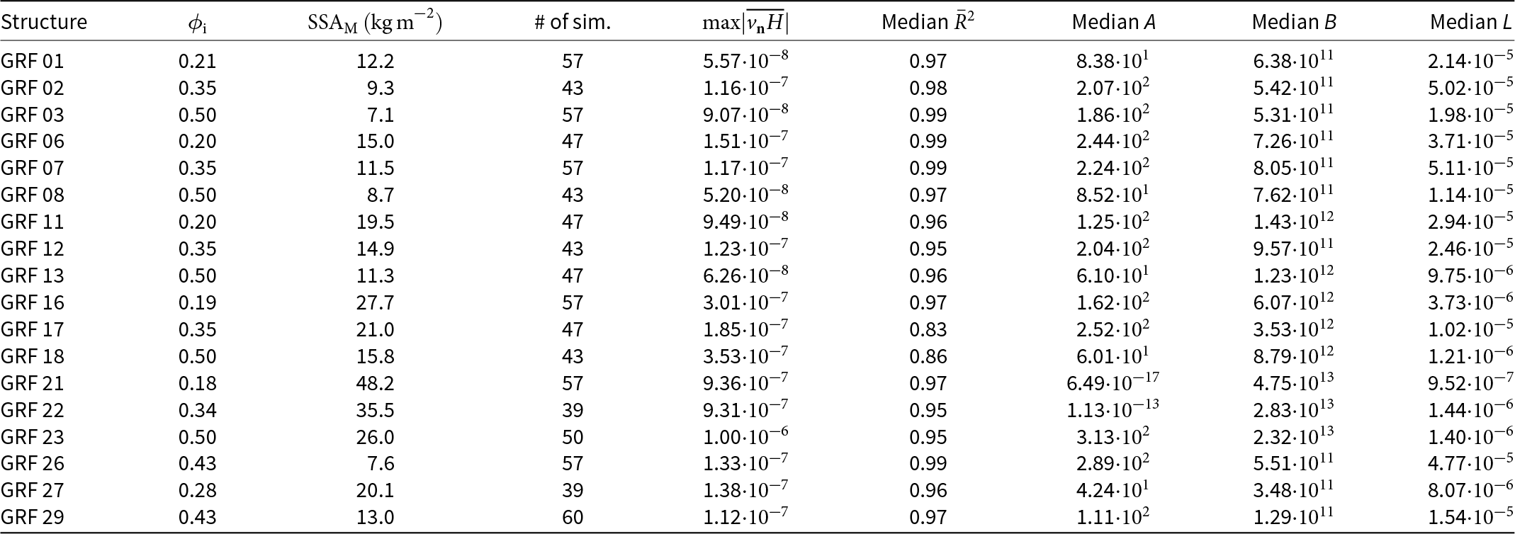


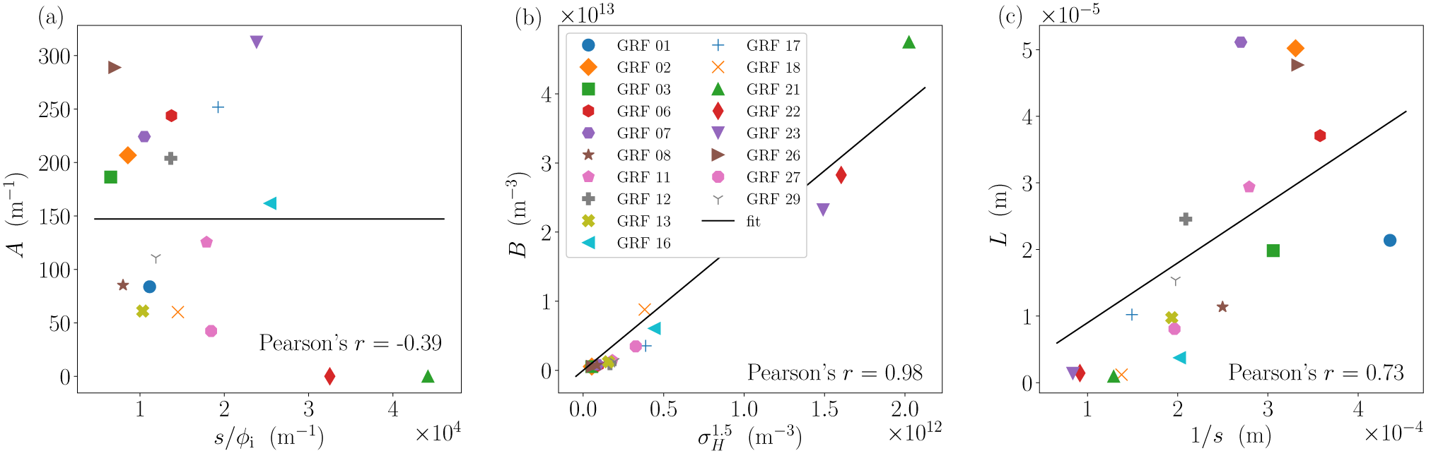


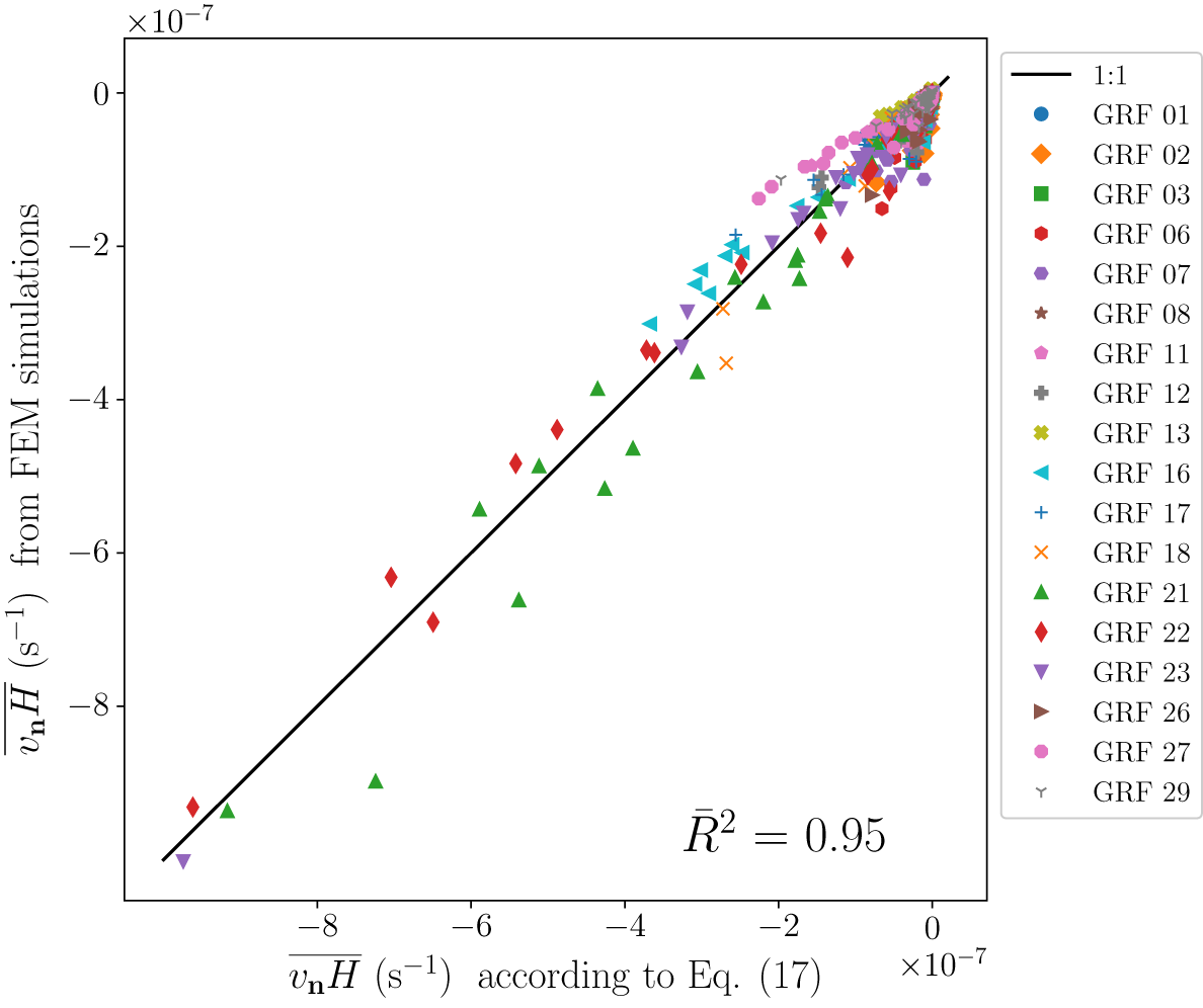

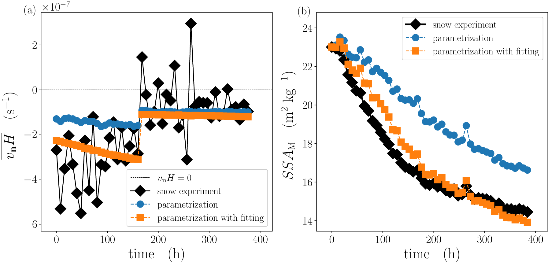

 Open access

