1. The Problem

The flow in the region close to the bottom end of a glacier is not adequately described by present theory. The theoretical treatments of glacier flow are all based on the approximation, which is valid far from the end, that the top and bottom surfaces of the glacier are almost parallel. If a model based on this approximation is extended towards the end, the top surface becomes more and more steeply inclined to the bed, and the approximation becomes useless before the end is reached.

To pose the problem more precisely, let us consider a glacier flowing down a uniform inclined plane in a state of plane strain, so that there is no component of velocity transverse to the main flow. Let some suitable boundary condition be imposed at the up-stream end and let us assume a definite distribution of rate of ablation (wastage by melting and evaporation) on the top surface; this could be specified as a function either of altitude or of the horizontal coordinate. We may presume that a steady state will eventually be reached, and we may ask what is the form of the steady-state profile and what is the distribution of stress and velocity. The problem is not completely posed until the properties of the material and the boundary condition on the bed have been specified. To choose these sufficiently realistically and at the same time have a tractable problem is a major difficulty. In these circumstances it seems useful to try to solve the problem for a plastic–rigid material with a constant flow stress (Reference HillHill, 1950, p. 128) and for a perfectly rough bed. This has the advantage of promising an exact (numerical) solution to a definite problem. A refinement would be to assume a more general flow law for the material (say a power law) and some more realistic boundary condition at the bed (perhaps based on Weertman’s theory of sliding), but the present paper does not go beyond plasticity with constant flow stress, although it does at the end consider some relaxation of the rough bed condition. We assume a horizontal bed, for the sake of definiteness; there is possibly no difficulty in introducing a sloping bed, but this has not yet been investigated in detail. An earlier but unsuccessful attempt to solve the same problem was made by Reference LliboutryLliboutry (1956).

2. Method

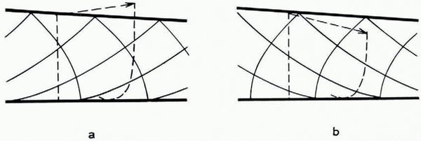
We do not know, a priori, whether a solution exists in which the material is plastic right up to the end, as in Figure 1a. For example, Figure lb shows another possibility where the material is deforming plastically up to a limiting slip-line and behaves rigidly beyond. Possibilities of this sort will be looked at later (p. 710–12); meanwhile we tentatively assume the existence of a solution that is everywhere plastic.

Fig. 1.

Hypothelical states at the end of the glacier

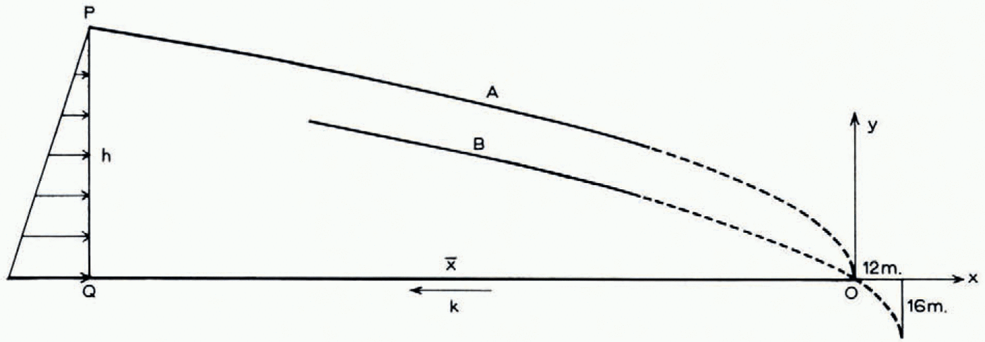
Take the origin at the end (Fig. 2) with Ox horizontal and Oy vertical. Reference OrowanOrowan (1949) has shown that at points far from the end an approximate profile may be found from elementary equilibrium considerations, as follows. Far enough to the center the surface slope is small and the hydrostatic pressure is large compared with k, the maximum shear stress. So the normal pressure acting across pq increases linearly from approximately zero at p to approximately ρgh at q, where ρ is the density, assumed uniform, and where pq = h. For unit thickness perpendicular to the diagram the force is then

.This must be balanced, since the motion is quasi-static, by the shear force kx acting across oq, where . Hence

or

where h ₀ = k/ρg. The constant h ₀, which is a characteristic length, has the order of magnitude 10 m. The condition for the surface slope to be small and for k to be small compared with pgh is the same, namely h ≫ _h0 The parabolic profile (1) is thus a valid approximation far from the origin.

Fig. 2.

Curve a: Orowan’s parabolic profile. Curve b: improved parabolic profile

When the stress and velocity distribution corresponding to this approximate parabolic profile is considered in more detail (Reference NyeNye, 1951), it is found that there are two possible approximate stress solutions in the plastic state, one corresponding to a compressive stress and strain-rate in the top surface (compressing flow) and the other to a tensile stress and strain-rate (extending flow). Both approximate solutions give a slip-line field consisting of parts of cycloids (Fig. 3a, b). The corresponding approximate velocity solutions are such that a vertical line becomes distorted after a small interval into a quadrant of an ellipse. In compressing flow (Fig. 3a) the flow lines diverge, and so there is an outward normal component of velocity at the top surface. For a steady profile there must therefore be ablation at the top surface. In extending flow (Fig. 3b) the flow lines converge. If the convergence is large enough there will be an inward normal component at the top surface, which, for a steady profile, must be compensated by accumulation (snowfall). If, on the other hand, the convergence were so small that the top flow line dipped less than the surface, extending flow could be associated with ablation. At the end of a glacier there is ablation—and, choosing between the two fields, it seems reasonable to start with that of Figure 3a (compressing flow) and to try to extend it to the right. However, as a numerical procedure this is not quite satisfactory, because the field of Figure 3a is not known exactly, but only to a first approximation in which the higher-order terms in h ₀/h are neglected. The field is only known exactly in the limit h → ∞.

Fig. 3.

Approximate cycloidal slip-line fields and velocity distributions for (a) compressing flow and (b) extending flow

To meet this difficulty we first take note of the close analogy (Reference NyeNye, 1951) between the present problem and a classical problem in plasticity theory, namely the weightless plastic material deformed between rough parallel plates. The slip-line field for this problem is shown in Figure 4 (Reference HillHill and others, 1951; Reference HillHill, 1950, p. 228). The two plates are forced together and the material squeezes out sideways to center and right. Two rigid wedges are center at the centre. Now it is easy to show that the same slip-line field is valid for the reverse problem where, in addition to the pressure on the plates, an excess pressure is applied to the ends of the block so as to force the plates apart. The material then flows inwards towards the centre, and all the velocities, shear stresses and pressure gradients are reversed in sign. Now allow the material to have weight. Any solution in the theory of plasticity for a weightless material may be transformed into a solution for a material with weight by leaving the velocities unchanged and by adding to the stresses at each point a hydrostatic tension ρgy, where ρ is the density, g is the gravitational acceleration, and y is the height of the point above a fixed horizontal plane (see e.g. Reference NyeNye, 1951, p. 556). The analogy we are trying to set up is between the slip-line field of Figure 3a and the region of the field in Figure 4 that is outlined by a broken line, with the material in this region moving from center to right. For the weightless material of Figure 4 there is an approximately linear decrease in pressure along ab. If ab is suitably inclined to the horizontal, when the transformation is made to the material with weight, the added hydrostatic tension, which also varies linearly along ab, just cancels the pressure; so ab, which is already free from shear stress, by symmetry, also becomes free from normal stress. It thus becomes the free top surface of Figure 3a. The two slip-line fields are not exactly the same, because while ab is exactly straight and parallel to the other boundary the top surface of the glacier is not. Nevertheless, the correspondence is close enough to suggest how the field of Figure 3a may be extended.

Fig. 4.

Slip-line field for a plastic material deformed between rough, parallel plates. Only one half of the block is shown. g is the centre. Shaded areas are undeforming

In computing the field of Figure 4 Hill and others deduced, by consideration of velocities, that the slip-line cd was straight and that the slip-lines in cde were radii and arcs of circles. They then extended the field to the right by a small-arc numerical process. They found that the field rapidly approached an asymptotic configuration in which successive slip-lines have the same shape; this is the well-known cycloidal slip-line field of Reference FrontardFrontard (1922) and Reference PrandtlPrandtl (1923). The approach is accompanied by discontinuities of diminishing strength; discontinuities propagating along the slip-lines are allowed by the hyperbolic natureof the equations, but they are very severely damped at each reflexion at the plates. Hill and others likened the behaviour to the operation of Saint-Venant’s principle in elasticity (although in elasticity there are no propagating discontinuities because the equations are elliptic). To solve the glacier problem we copy this procedure. We start with a field of radii and arcs of circles and extend it to the right. The expectation is that, so long as the field is started in a way consistent with the plasticity equations, the details of how it is started will not matter—it will quickly settle down to the approximately cycloidal field of Figure 3a. We can then continue the numerical computation to find the field in the tip region of the glacier, where the cycloidal field is no longer even approximately valid.

Accordingly, the problem is set up as in Figure 5. The material obeys the equations of plasticity with constant flow stress k, and is weightless. On the horizontal plane y = 0 we assume τ _xy = k. On the upper surface, whose shape is to be calculated, there is no shear traction but there is a normal pressure proportional to altitude ρgy (ρ being the density when we later transform to a material havingweight). The center-hand boundary ca is taken as straight with the angle

, where α ₀ is a constant to be fixed later. On ca a shear traction k is applied in the sense shown; ca is then a slip-line. Since the top surface must meet ca at an angle of , its downward slope at a must be α ₀. The normal pressure on ca is chosen to be uniform to satisfy the plasticity equations, and we give it the value ρgH+k to keep the stress continuous at a, where H is the y coordinate of a (the principal stresses at a are −ρgH and −ρgH−2k). On transforming to a material of density ρ we add a hydrostatic tension ρgy everywhere. This frees the top surface of stress, as required, and gives a pressure on ac of ρg(H−y)+k.

Fig. 5.

The slip-line field is started as radii and circular arcs in cas and extended by a small-arc process to the end of the glacier. Only selected slip-lines are shown. The profile and slip-lines are to scale (drawn by the computer) for a starling height ak of 10h ₀ ( ≃ 100m.), this rather small starting height being chosen for clarity in the figure; larger starting heights and therefore longer glaciers were used for the computations reported in the paper. The boundaries shown between fields I, II and III are not of course sharp

The normal velocity on the lower surface is taken to be zero. On the upper surface the outward normal velocity is prescribed to be positive and is given as a function of x or y. In the actual computation reported here it was taken as uniform with the value U/√2, where U is a constant. If the rate of ablation were also uniform and equal to U/√2, there would be a steady state. The normal velocity across ca will be determined later.

The center-hand boundary and the conditions on it have been chosen to satisfy the plasticity equations. Since the shear stress on the bed and on ca is k, c is a stress singularity. The slip-line field is begun as radii and circular arcs in cab. The sense of the shear tractions on ca and cb shows that the radii are α-lines and the arcs are β-lines (Reference HillHill, 1950, p. 134). In continuing the field we expect, by analogy with the parallel-plate problem, to find three regions. a field (I), analogous to the edge field in the parallel-plate problem, will be followed by an approximately cycloidal field (II), described by the approximate analytical solution valid for small surface slopes. As the solution is further extended the surface slope will become large and we enter the tip region (III). Field I is of no particular interest; it depends on the center-hand boundary conditions which were chosen arbitrarily in order to start the solution in a simple way. Field II should agree with calculation and so checks the method. Field III is the objective of the computation.

The value of α ₀ and the length of ca, which we denote by r, are thus far arbitrary r must be chosen fairly large, say >10 _h0, for otherwise field II will not be attained before field III sets in; and in this case field III would depend on the starting conditions, which we do not want to happen. Apart from this, the length of ca ought not to matter so far as field III is concerned. The choice of α ₀ is more difficult. If α ₀, is chosen very far from the values that the surface slope will take in field II we can expect severe oscillations in field I. We want to choose α ₀ so as to make the transition from I to II reasonably smooth. If ca is large enough, field III should not depend on the precise value of α ₀. However, it turns out, as we now show, that there are other restrictions on α ₀ that may be found by considering the small-arc process for calculating the slip-lines.

Referring to Figure 5, ef is a typical -line; suppose the field to the center of this slip-line is known (ef could be, in particular, the circular arc ab). If eh is a small arc we can find the position of g (Appendix A) by using the plasticity equations and the top boundary condition. By the usual small-arc process the slip-line gm may then be found, where m is on the α-line through f. Obviously m must lie on or above the lower boundary or the process will fail. So fm, which is tangential to the bed at f, must not curve downwards. The necessary and sufficient condition for this is that hg should not be concave downwards, by Hencky’s first theorem (Reference HillHill, 1950, p. 136). (The theorem shows that the change in the angle of the slip-lines between h and g is the same as the change between f and m.) In the critical case fm, and therefore hg, are straight. Let us see what this implies.

On the top boundary the principal stresses for the weightless problem are −ρgy, −ρgy−2k. So on the boundary the mean compressive stress p equals ρgy+k. By the plasticity relations along the slip-lines (Reference HillHill, 1950, p. 135)

where ϕ is the angle of the α-line to Ox measured anticlockwise. Applying these relations to the arcs, hg and he (Fig. 5 inset) and eliminating p _h we find

where δ _α ϕ and δ _β ϕ are the increments in ϕ along hg and he. Using the boundary values of p and putting y _e−y _g = Δ and h ₀ = k/ρg, this becomes

In the limit of small arcs he = hg = δ, say. Divide equation (4) by δ to give

or, in the limit,

where α is the surface slope and R, S are the radii of curvature of the slip-lines, defined in the usual senses by

The condition for the small-arc process to work may now be written as 1/R ≧ 0, or, by (5), as

We shall make two applications of this condition, one now and one later. At a in Figure 5, S = −r where ca = r. So (6) gives

Thus, if α ₀ is chosen too small, zero for instance, the initial α-element pq will curve downwards and the process will fail. If, on the other hand, α ₀ is chosen much too large, pq will curve upwards rather sharply. It seems likely that, in this case, the next or a later element of the α-lines will curve downwards, thus transferring the breakdown to a later step—but this has not been studied. To avoid such oscillation and consequent breakdown α ₀ was chosen so as to satisfy the equality sign in (7). It is readily shown that, in terms of H(= y _a) rather than r, condition (7) may be written

The length of the glacier is known a priori if we assume that the shear traction k is maintained on the horizontal bed right up to the end. (We shall find later that this assumption may not be true, but it still provides a convenient practical way of fixing an origin of x in advance.) A balance of horizontal forces (Appendix B) then gives

where L = ko (Fig. 5), which is essentially the same as equation (1) except for the last term. It is of interest that (9) is independent of how α ₀ is chosen. A formula for co rather than ko would not have this property.

Small-arc process. Having chosen r and α ₀ the numerical process is started at a in Figure 5, and is designed to find the next β-line to ab. It is then repeated to find successive β-lines. The details are given in Appendix A. The computations were programmed in ALGOL for an Elliot 503 computer (Computer Unit, Bristol University). H was taken as 20h ₀ (L = 220h0) and the arc ab was divided into at first 20 intervals and later into 40 intervals. Further computations were made for H = 20√2h ₀ (L ≃ 428h ₀) to check that field III was independent of H. α ₀ was fixed by the equality sign in (8). The first α-element pq is then straight in the limit of small arcs. With the finite arcs used it did in fact curve upwards slightly (for 20 intervals and H = 20h ₀, ϕ _a = 0.7378, ϕ _p = 0.7194, ϕ _q = 0.7225). This difference between ϕ _p and ϕ _q is preserved exactly down to the bottom element BS, so S is slightly above the bottom, as required.

The procedure computed the slip-lines in fields I and II satisfactorily. For 20 intervals the computation time was between 0.2 and 1 sec. for each β-line (depending on how much information was placed in the backing-store for later use).

Break-down near the terminus. Near the terminus the computation of the slip-line field breaks down because the typical arc hg (Fig. 5) begins to curve downwards. fm therefore curves downwards too and the computation must stop. We can see that this is inevitable, as follows.

First we show that the curvature of the β-line at f (Fig. 5) is infinite (Reference HillHill and others, 1951, p. 52). With origin at f the α-line through f is, say,

The curvature of the β-line at f is then

which is infinite whatever the value of n.

Now, by Hencky’s second theorem (Reference HillHill, 1950, p. 138), as one passes along an aline the radius of curvature of the successive intersecting β-lines changes by the distance traversed. Since the radius of curvature of the β-line at f is zero, the radius of curvature of the β-line at j is fj, where fj is the arc length. So criterion (6) for the α-line through j to curve upwards may be written

(S being negative). As we approach the origin

, because assuming the material is plastic up to the end this is the only value that is compatible with a free top surface and a bed which is a surface of maximum shear stress. So the criterion becomes

But from Figure 5 it is clear that fj must continually decrease; so when fj becomes less than 2h ₀, if not before, we must expect the computation to fail on the β-line through j. It does so in fact when x at j is −0.3h ₀, that is about 3 m. from the end. The break-down thus occurs extremely close to the end, in a region where the result of the computation may not be of physical interest—for in real glaciers factors outside those in the present model may dominate the scene within a few metres of the ice edge (irregularities in the rock bed and in ablation rate, and melting on the bottom surface). Nevertheless, the failure cannot be dismissed, because while the slip-line field remains open-ended we cannot be sure that it is part of a valid solution to any physical problem.

The difficulty may be met by modifying the lower boundary. One way is arbitrarily to make the lower boundary follow the last valid α-line, or any preceding α-line. But we can solve a problem closer to the one originally posed if we continue the slip-line field further to the right in the following way. When the point is reached in the computation at which the element fm (Fig. 5) curves downwards, instead of declaring the method to have broken down, we redefine the lower boundary to follow this slip-line. Thus, in Figure 6, ab curves upwards and a new point c is taken as the beginning of a new α-line. But cd is found to curve downwards, so the bed, which is horizontal up to c, is made to follow the slip-line. Clearly, there is one less arc element in fd than in ec; so as successive β-lines are computed elements are lost, one for each step, and the field finally terminates at g. This procedure results in a full solution to a problem that is very close to, but not identical with, the original one. The y-coordinate of g is −0.00336h ₀ (see Table I); thus the bed curves down by 3 cm. over the final 3 m. of its length. For all practical purposes, but not in theory, the problem has been solved for a horizontal bed.

Fig. 6.

Computed slip-line field (to scale) very near the end of the glacier. Only selected slip-lines are shown. c is the critical point at which the bed ceases to be horizontal. Inset: final triangular element, not to scale

Table I

Values at Extremity of Glacier

The lower boundary of the plastic region is an envelope of slip-lines up to c (Fig. 6), but is a slip-line from c to the end; the field in the parallel-plate problem (Fig. 4) behaves in just the same way, ef being an envelope and fg a slip-line.

Velocities. The velocity field is computed from right to center as in the corresponding parallel-plate problem. The boundary condition on the top surface is that the outward normal component of velocity is U/√2, a constant; or, in terms of the velocity components u, υ parallel to the slip-lines,

On the lower boundary υ = 0. The fundamental equations governing the variation of u and υ along the slip-lines are (Reference HillHill, 1950, p. 136):

At g in Figure 6 the boundary conditions give u = U, v = 0. Since v = 0 on the α-line cg, it follows from (II) that du = 0, and thereforeu = U on cg. In particular u _H = U, υ _H = 0. At 1 we have, from (12) applied to hi,

and, from the boundary condition,

The ϕ values being known, these two simultaneous equations may be solved for u ₁ and υ ₁. In a similar way the velocities are computed at j, k and l, and so on for successive β-lines, up to the line cb … e. The next point a is computed by using (11) along ab together with υ _a = 0. And so the computation continues up to the circular arc ab in Figure 5. Within cab (Fig. 5) the α-lines are straight. So, from (11),uis constant along the α-lines. Therefore u = u(ϕ). Introducing this relation in (12) with υ = 0 on cb, shows that, within cab, υ = υ(ϕ). Therefore υ is constant on ca. The functions u(ϕ) and υ(ϕ) are known from the values of u and υ on ab. In particular, the constant value a υ on ca is found from the computed value of υ at a. Thus, to maintain the outward flow across the top surface of the glacier, material has to be fed in across ca at a uniform rate whose component normal to ca is −υ _a. The direction of motion of material just after crossing ca (on a radial line through c) is uniform and not, in general, parallel to the bed. c is a velocity singularity.

In the parallel-plate problem of Figure 4 the normal velocity across cd has to be compatible with a rigid-body motion of the material to the center of cd. That is why cd is straight—because then the normal velocity across it comes out to be uniform and therefore compatible with rigid-body motion. In the glacier problem (Fig. 5) ca was chosen straight and the normal velocity across it likewise comes out to be uniform, as we have just seen. We could then, if we wanted to, have rigid material to the center of ca. But whereas in the parallel-plate problem this feature is essential, in the glacier problem the conditions to the center of ca are center unspecified. The center-hand boundary condition in the model is not supposed to represent reality; it is merely a mathematical device for starting the slip-line field, and therefore further discussion of how it might be realized physically would be academic.

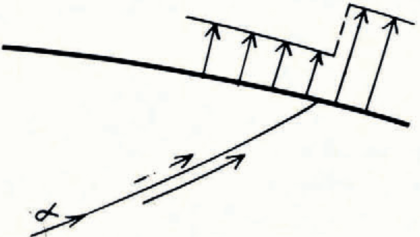
The computation described was made for a uniform normal velocity on the top surface, corresponding to a uniform ablation rate in the steady state. But the same slip-line field should be valid even when this velocity is allowed to be non-uniform. The velocity field could be computed by an identical method, except that U in equation (10) would be a function of position. There is, however, a further condition to be satisfied: that the sign of the plastic work should be everywhere positive. For U uniform there is no reason to suspect that the computed solution does not meet this condition; but if U is non-uniform it could be violated—as may be seen as follows. A discontinuity in U in the sense shown in Figure 7 would lead to a discontinuity in u across an α-line as indicated. The sense of the discontinuity in u is opposite to the sense of the shear stress, and so negative work is done. The slip-line field is therefore invalid for such a distribution of U. (A discontinuity of the opposite sense is compatible with the slip-line field.) If attention is confined to continuous variations there is presumably a critical gradient of ablation rate beyond which the slip-line field is invalid. The critical case evidently occurs when ablation decreases with altitude—which is, of course, unfortunately, the variation normally found. Very rough calculation shows that the solution is likely to fail when the ablation gradient exceeds about 10 per cent in 0.1 km., measured along the glacier surface—so the solution appears to have a useful range of validity.

Fig. 7.

A discontinuiy in ablation rate is associated with a discontinuity in velocity across an α-line

3. Results

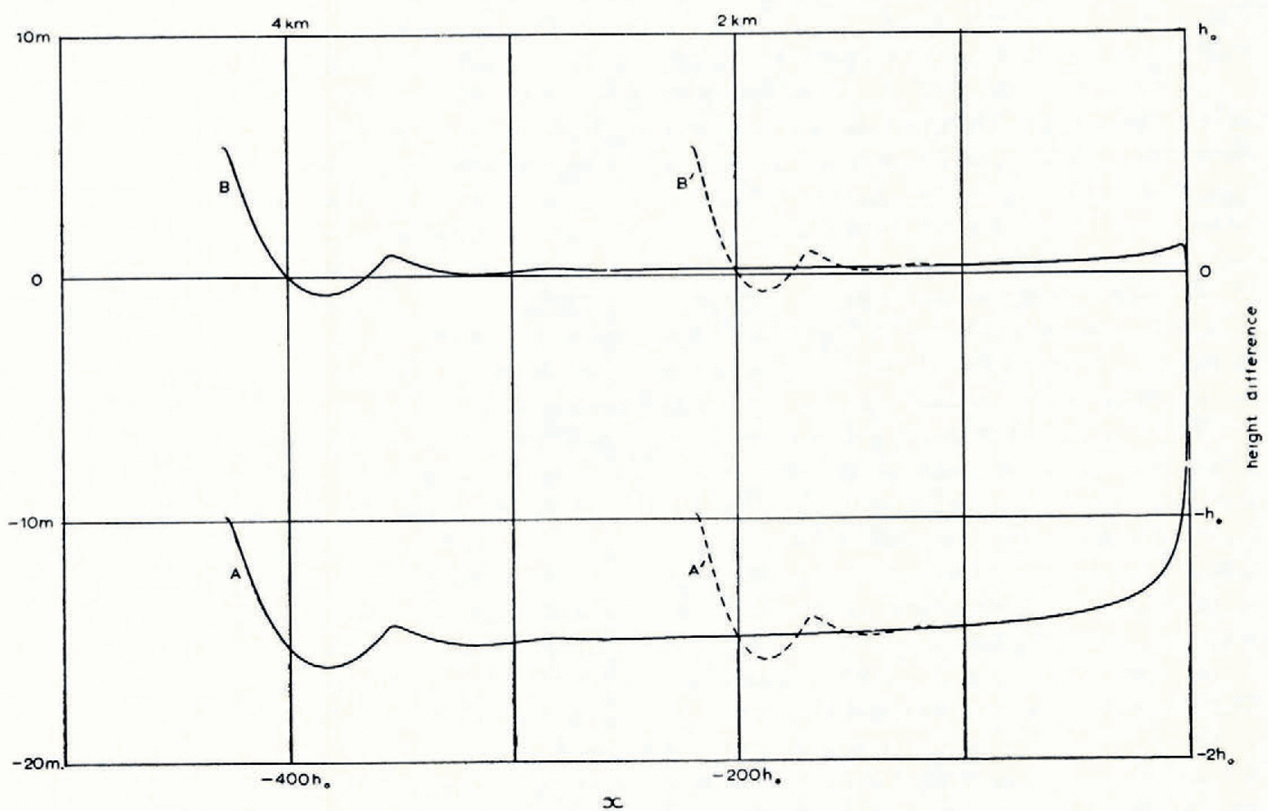
(i) Profiles. Let us look first at the computed profile and compare it with the Orowan parabola of equation (1). The lower curves in Figure 8a show h (computed) —h (Orowan) plotted against x for two different starting heights. The computed profiles oscillate at first in field I but, as expected, they rapidly settle down in field II to a single steady curve that lies about 1.5h ₀ below the parabola.

We can improve on the Orowan parabola as an analytical approximation by replacing the linear distribution of normal pressure on pq (Fig. 2) by the more accurate distribution given by the cycloidal slip-line field (Reference NyeNye, 1951). The latter gives an average pressure on pq, of

, in contrast to the value of assumed before. Balancing horizontal forces then gives

which, by making the substitutions

may be written

Thus the improved profile (13) is exactly the same parabola as that of equation (1), but with its apex shifted downwards by

. and to the right by . (Fig. 2). It passes through the origin O with a slope of 2/π ≃ 0.64.

By using this modified parabola the agreement with the steady computed profile in field II is much improved (Fig. 8a, upper curves), the difference being typically 0.04h ₀ ≃ 0.4 m.

Fig. 8a.

Curves a, a’: h (computed)—h (Orowan) plotted against x for two different lengths of glacier. Curves b, b’: h (computed)—h (improved parabola) plotted against x,for two different lengths of glacier

The same argument provides an improvement on the well-known approximate formula obtained by considering the shear stress on the bed, namely

where α is the angle of the top surface. For, by considering the equilibrium of the material between x and x+dx, we have

where

, neglecting terms of order ρgh(k/ρgh)². The upper sign refers to the case in hand (compressing flow), and the lower sign to extending flow. Putting dh/dx = −tan α and solving for k gives

neglecting terms of order ρghα ³.

The first approximation (14) leads on integration to the Orowan parabola (1), while the second approximation (15) with the upper sign leads to (13). It will be seen that the formulae for the two types of flow differ in the second approximation but not in the first. When applied to the computed profile, the right-hand side of (14) gives values about 10 per cent too low in field II. This is the order of error expected (for the proportional error is of order α and at x = −100h ₀, for example, α ≃ 0.08). On the other hand, formula (15) with the upper sign brings the error down to about 1 per cent in field II (Fig. 8b). (Figure 8b shows once again how the two different starting heights produce curves that oscillate in field I, but then settle down to a common steady curve.)

Fig. 8b.

Test of theoretical relation between h and α. The right-hand side of formula (15) is plotted against x, for two different lengths of glacier (full curve: starting height 20√2h ₀; broken curve: starting height 20h ₀)

It should be emphasized that formulae such as (14) and (15) cannot hold in all circumstances. For example, (15) is in error by 90 per cent in field I, even though a is less than 0.07. This is because there does not exist, in general, any unique relation between h and α. On the contrary, both are determined at each x by the boundary conditions. The fact that formulae (14) and (15) give definite relations between h and α that are independent of x, and therefore independent of the proximity of the center- and right-hand boundaries (provided they are distant), is an unobvious result that is to be regarded rather in the same way as Saint-Venant’s principle in elasticity. The formulae hold when the steady field II conditions have become established.

The same principle no doubt applies outside the realm of constant flow-stress plasticity. The generalization of field II to a more general flow law is carried out in (Reference NyeNye, 1957). The σ _x distribution is no longer elliptical and the correction term in equation (15) will then need modification. Thus, the correction term in (15) is only applicable in constant flow-stress plasticity. The leading term, on the other hand, has a wider relevance if k is interpreted as the shear stress on the bed.

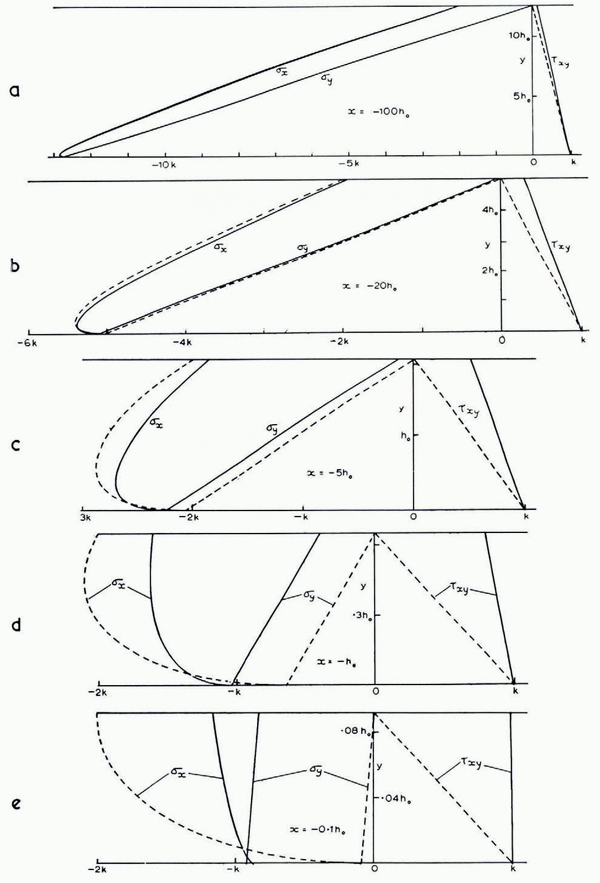
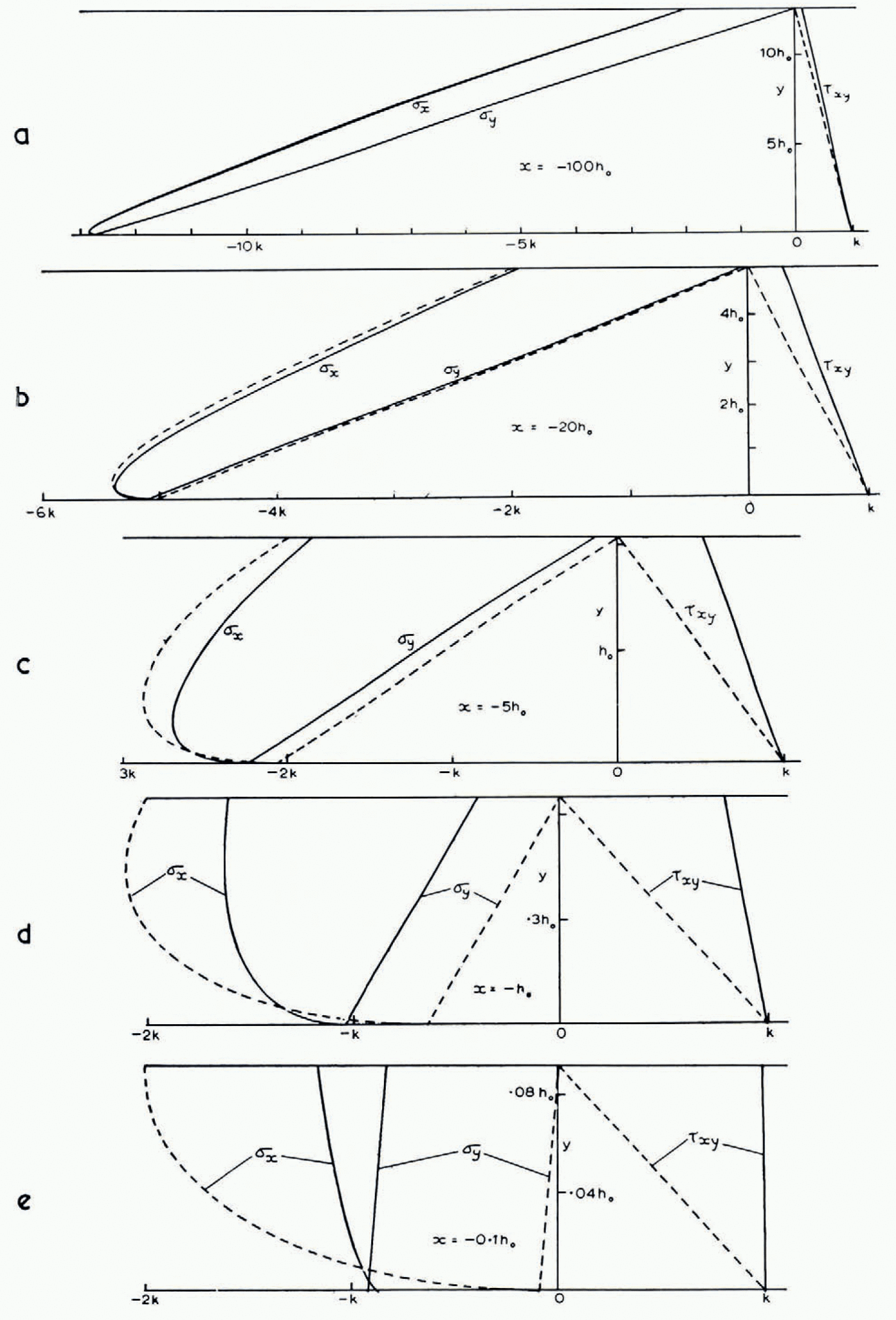
(ii) Stresses. The computer was programmed to evaluate p, ϕ, u, υ at all the grid points of the slip-line field. It also evaluated the distribution of the Cartesian stress components σ _x , σ _y , τ _xy and velocity components u _x , υ _y for certain fixed values of x, by interpolation between grid points, and compared them with the values given by the approximate analytical solution. For example, Figure 9a shows the three stress components at x = −100h ₀. (The difference between results for the two starting values H = 20h ₀ and 20√2h ₀ is nowhere more than 0.007k.) The approximate analytical solution (Reference NyeNye, 1951, p. 558) is

and neglects terms of order h ₀/h. The stresses predicted by (16) should therefore agree with the computed stresses to order (h ₀/h)k = 0.08k. This expectation is confirmed; the two curves for σ _x and the two for σ _y are indistinguishable on the scale of the figure. τ _xy at the surface shows the greatest departure, being 0.140k compared with zero.

Figure 9a to e show how the departure of the approximate solution (broken lines) from the computed solution (full lines) grows towards the terminus, until at x = −0.1h ₀ there is no longer any resemblance. It is striking that σ _y and τ _xy which are linear in y in the approximate solution, remain linear in y to high precision in the computed solution, even as close to the terminus as x = −h ₀ and x = −0.1h ₀. σ _y is in fact very closely approximated by

Fig. 9a to e.

Cartesian stress components at 5 selected values of x. Full curves: computed; broken curves: approximate analytical solution (16)

throughout the entire range. In the equilibrium equation

the first term is zero on y = 0 by the boundary condition τ _xy = k (we exclude the end region x > −0.3h ₀ where the bed ceases to be horizontal). So, near enough to y = 0, σ _y will necessarily be exactly represented by equation (17). But for the other y (17) cannot be exact because it would imply ∂τ _xy /∂x = 0 for all y, which is by no means true. In other words, the non-linearity of σ _y with y, which is barely perceptible in the graphs, is essential for satisfying the equations.

(iii) Velocities. Figure 10a to e show the Cartesian velocity components u_x , υ _y as computed (full lines), and as calculated (broken lines) from the approximate formulae (Reference NyeNye, 1951, p. 562)

Fig. 10a to e.

Cartesian velocity components at 5 selected values of x. Fill curves: computed; broken curves: approximate analytical solution (18)

(q = discharge, α = surface slope, u_n = velocity normal to the surface,

mean u_x , s = distance along the surface from the end). The difference from the approximate analytical solution is quite small at x = −100h ₀ and grows towards the end, as expected. Nevertheless υ _y remains approximately linear in y, so that the vertical strain-rate remains approximately uniform with y even down to x = −h ₀. (At x = −0.1h ₀, υ _y becomes very small and negative to follow the downward sloping bed.) The variation of u_x with y, which is initially elliptical, becomes more nearly linear towards the end, but even at x = −0.1h ₀ it is still appreciably non-linear, so that homogeneous simple shear would not be a very good representation.

(iv) Strain-rates. It is of interest to compute the rate of compression (i) along the bottom and (ii) along the top surface. Both distributions (Fig. 11a, b) show a discontinuity in field I that emanates from A in Figure 5 and propagates with diminishing intensity along the slip-lines ab, br, etc. In the approximate solution (18) the strain-rate component ∂u _x /∂x at given x is independent of y, and in agreement with this the two curves in Figure 11a run close together in field II. In field III the strain-rate on the bottom reaches a maximum compression of 0.11 U/h ₀ at about x = −2.7h ₀. (For example, if h₀ = 10 m. and U = 10 m./yr., which corresponds to an ablation rate of 7.1 m./yr., this is a compression of 11 per cent per year at 27 m. from the end.) In the extreme tip region −0.3h ₀ ≦ x ≦ 0, where the bed has been made to follow a slip-line, the strain-rate on the bed is necessarily zero.

Fig. 11a.

Compressive strain-rate along the bottom (broken line) and along the top surface (full line) planed against x. Starting height 20h₀. Numerical scales inserted for U = 10 m./yr. (ablation rate 7.1 m./yr.) and h ₀ = 10 m.

Fig. 11b.

As Figure 11a but scale of x magnified to show detail near the end

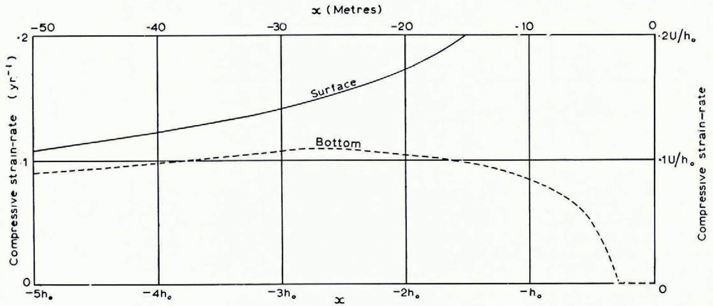
The compressive strain-rate in the surface rises steadily (Fig. 11a, b) in fields II and III and goes up very steeply near the end. Computed values of the surface compression-rate

at the extreme end are shown in Table I (p. 702). A value of about 3.2U/h ₀ is indicated in the limit as H → ∞ and n → ∞.

Theoretically, it may be shown (Appendix C) that

, where S₀ is the radius of curvature of the final β-line (of infinitesimal length) at the end. But in Figure 6 the radius of curvature of the β-line at c is zero, by the argument given previously, and hence, by Hencky’s second theorem, S ₀ is the arc-length cg. Thus . The computed value of is consistent with this result.

We shall refer to observational evidence on the surface strain-rate at the end of a glacier in Section 5 (p. 712).

4. Possible End Configurations

Having discussed a particular solution in which the glacier deforms right up to the end, we may now consider some other possible terminations. Provided the upper and lower boundary conditions continue to hold, and provided the material remains plastic, the slip-line field must continue in the way we have described. One way of terminating it, as mentioned earlier, is arbitrarily to make the bed follow first the envelope of the α-lines and then a particular α-line of the solution. All boundary conditions are then automatically satisfied. The solution described is an example of this where the particular α-line is the one passing through the critical point c in Figure 6. But any other preceding α-line, such as pq in Figure 1b, could just as well have been chosen as the bed.Footnote *

A possible objection to solutions of this type is that they assume that the shear traction on the lower boundary remains equal to the critical value k right up to the end. It is commonly observed that at the end of a glacier the ice does not make contact with the rock bed over its whole area, presumably because the normal pressure is insufficient. But further up the glacier, as the normal pressure increases, the proportion of contact supposedly approaches 100 per cent. Within a metre or so of the ice edge the ice is often, but not always, completely out of contact with the bed; but we distinguish between this cantilevered region, which is considered further in Section 5, and the more extensive region where contact is less than 100 per cent. As a rough representation of the friction law that results in this latter region we may take

where τ is the shear traction and p is the normal pressure. μ is a coefficient of friction, but would not necessarily be equal to such a coefficient measured on a laboratory scale.

Thus, if p falls below the critical value k/μ as the end of the glacier is approached, we cannot expect the full plastic friction to develop, and the boundary condition τ = k on the bed must change. A detailed examination shows that it is not possible to extend the slip-line field beyond this critical point by going over to the boundary condition τ = μp. Therefore, beyond this point the material on the bed cannot deform plastically. According to a general theorem in plasticity theory, the deforming plastic region must be bounded by a slip-line (Reference HillHill, 1950, p. 151), across which the tangential component of velocity may be discontinuous. We shall find that there must be such a discontinuity, and therefore the bounding slip-line cannot be a β-line, because the condition υ = 0 on the bed precludes a discontinuity there. It must be an α-line, such as pq in Figure 1b, and p will be the point where p falls below the critical value k/μ Now in the computed, fully plastic, solution with the almost horizontal bed, p falls as the end of the glacier is approached, reaches a minimum value at c in Figure 6 of 0.875k(x = −0.3h ₀), and then rises gradually to k. So if μ > 1/0.875, that is μ > 1.14, the normal pressure is always enough to produce τ = k. We must then expect 100 per cent contact right up to the end (but see Section 5). The conclusion is that the solution described is valid under the friction law (19) provided μ > 1.14. Along other α-lines, p never falls below 0.875k, and so for μ > 1.14 the bed can equally well be placed along any one of them. (Incidentally, p is slightly less than k in a region that starts on the bed at x = −0.8629h ₀ and extends to the end of the glacier; this means that the principal stress component approximately normal to the glacier surface is slightly tensile in this region.)

If μ < 1.14, on the other hand, a point p is reached on the horizontal bed where the normal pressure becomes insufficient to maintain τ = k and the deforming plastic region must be terminated on the α-line pq. It is natural to suppose that the remainder of the glacier to the right of pq moves rigidly, but this does not, in fact, provide a consistent solution, as can be seen as follows. Suppose the bed is exactly horizontal up to the end (as pr in Fig. 1b) and that the upper surface qr is subject to the same ablation rate as everywhere else. The velocity in pqr is then supposedly uniform and parallel to the bed, and, in order to maintain a steady profile, qr must be straight—but there may, in general, be a discontinuity in the slope of the profile at q. It turns out on detailed examination that a balance of forces on the section pqr, both horizontal and vertical, now allows the angle prq to be determined (the tractions on pq are known, and the average tangential traction on pr is μ times the average normal pressure). The discontinuity in surface slope at q is then calculable. Now υ, the velocity along the β-lines, must be continuous at q. The velocity normal to the surface is also continuous by the boundary condition. Therefore u, the velocity parallel to pq is discontinuous across pq. Such a discontinuity across a bounding slip-line is usual in plasticity solutions, but it is, of course, necessary that its sense should be the same as that of the shear traction across the slip-line, for otherwise negative work is done. The fact is that in the present problem the surface turns out to be re-entrant at q, and the resulting discontinuity of u is then of the wrong sign. Therefore the postulate that pqr behaves entirely rigidly must be false. The correct solution for μ < 1.14 is unknown. Presumably there is at least one plastically deforming region within pqr.

In brief, for μ > 1.14 we have a self-consistent solution for a bed which is for all practical purposes, but not exactly, horizontal.Footnote * For μ < 1.14 the complete solution is not known, but only up to the limiting slip-line pq, which acts as a thrust plane.

5. Validity of the Model near the End

On the bed within a few metres of the end of a glacier there will be melting because radiation can penetrate the ice and be absorbed at the ice–rock interface. This, and further melting by conduction of heat through the rock, cause the ice to lose contact with the bed, quite apart from the effect considered in the last section. Since our model ignores this effect (as well as the natural irregularities in the rock bed and the effects of moraine carried by the ice) it cannot be realistic within a few metres of the ice edge.

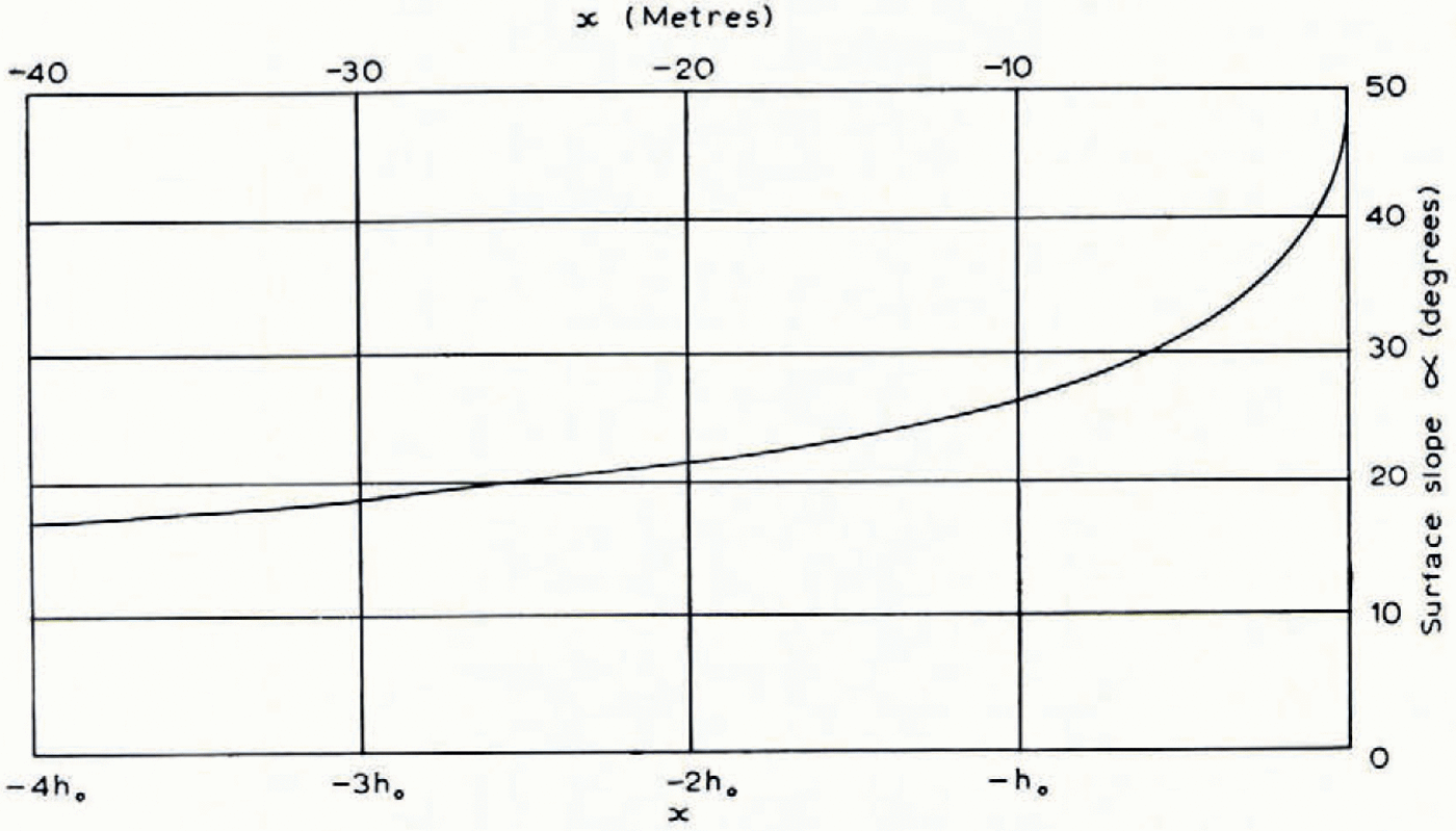
At distances of more than a few tens of metres from the ice edge, however, it appears to be a useful representation. It might at first be thought that this cannot be so because the model gives a terminus angle of 45°, whereas the terminus angles of most temperate glaciers are considerably smaller, say 10° to 20°. But in Figure 12 the angle of the surface, α, is plotted against distance from the end, taking h ₀ = 10 m., and it will be seen that the angle diminishes rather quickly away from the end. If one excludes the last 10–20 m., on the grounds that contact with the rock bed is not complete, the angle of the surface takes values consistent with observation. One may also remark that most glaciers at present are retreating; the terminus angles would probably be greater if they were stationary, as assumed in the model.

Fig. 12.

Angle of the surface α plotted against distance from the end.

The surface strain-rates shown in Figure 11 a and b may now be compared with Reference GlenGlen’s observations (1961) on Austerdalsbreen. He found a fluctuating compressive strain-rate averaging 0.1 yr.⁻¹ over the last 220 m., and noted that it was remarkable that the compression was maintained down to his last measured stake interval: over the interval 3 to 19 m. from the end of the glacier there was still a compressive strain-rate of 0.06 yr.⁻¹. He concluded that strain occurred down to the point where the ice lost contact with the bed.Footnote * Figure 11a and b shows that in the plastic model compressive strain-rates of 0.05 to 0.2 yr.⁻¹ occur in the surface in the range of x from −200 m. to −15 m. The Austerdalsbre results are therefore quite consistent in order of magnitude with the conclusions of plasticity theory. The very high compression rates in the theoretical model, up to ~3yr.⁻¹, only occur within the last few metres of the ice edge, and are not attained in practice if bottom melting frees the ice from the bed. It might be worth while looking for them at places where good contact is maintained.