2.1. The model and its averaging

Notations and general assumptions. As usual, ${\mathbb{R}}$ is the set of real numbers, with ${\mathbb{R}}^\ast_+$ the set of positive real numbers. The space ${\mathbb{R}}^d$ , where $d\geq2$ is an integer, is endowed with the Euclidean distance d with corresponding norm $\|\cdot\|$ and associated scalar product between points x and $\tilde x$ in ${\mathbb{R}}^d$ denoted by $x\cdot\tilde x$ . ${\mathbb{N}}$ is the set of positive integers. We let $\lambda_d$ denote the Lebesgue measure on ${\mathbb{R}}^d$ . In the following, ${\textbf{Y}}=\{y_1,\ldots,y_{|{\textbf{Y}}|}\}$ is a finite set of cardinal $|{\textbf{Y}}|$ . The real $T>0$ denotes a finite time horizon.

Description of the model. Let $({\Omega},\mathcal{F},(\mathcal{F}_t)_{t\in[0,T]},{\textbf{P}})$ denotes a filtered probability space. We define a PDMP in the Euclidean-mode setting as a càdlàg stochastic process $(X(t),Y(t))_{t\in[0,T]}$ on the state space ${\mathbb{R}}^d\times{\textbf{Y}}$ as follows. The continuous component, X, takes values in ${\mathbb{R}}^d$ and has continuous paths, while the discrete one, Y, takes values in ${\textbf{Y}}$ . The dynamic of the continuous component is defined by the family of d-dimensional vector fields $F_y$ indexed by $y\in{\textbf{Y}}$ . The behaviour of the discrete component is determined by the family of rate functions $q_{yz}$ for each $(y,z)\in{\textbf{Y}}^2$ , describing the jumping rate between states y and z. The sample paths of a PDMP $(X(t),Y(t))_{t\in[0,T]}$ are then constructed in the following way.

For any $(x,y)\in{\mathbb{R}}^d\times{\textbf{Y}}$ we define the survivor function

\begin{equation*}S_{(x,y)}(t)\;:\!=\; \mathrm{e}^{-\int_0^t q_y(\phi_y(x,s))\,\textrm{d} s},\quad t\geq0.\end{equation*}

This is the survivor function of a non-negative random variable. Let $\tau_0=\sigma_0=0$ and $(X(0),Y(0))=(X_0,Y_0)$ be a ${\mathbb{R}}^d\times{\textbf{Y}}$ -valued random variable. Assume that the process is built until time $\tau_{n-1}$ , for $n\in{\mathbb{N}}$ . Then we can define a random variable $\sigma_n$ , the inter-jump time, satisfying

\begin{align*} {\textbf{P}}(\sigma_n>t\mid (X_{n-1},Y_{n-1})=(x,y))=S_{(x,y)}(t),\quad t\geq0.\end{align*}

We define the nth jump time by

\begin{align*} \tau_n\;:\!=\; \tau_{n-1}+\sigma_n\end{align*}

and we set

\begin{align*} (X(t),Y(t))\;:\!=\; \begin{cases}(\phi_{Y_{n-1}}(X_{n-1},t-\tau_{n-1}),Y_{n-1})&\text{for } \tau_{n-1}\leq t<\tau_n,\\[5pt] (X_n,Y_n)&\text{for } t=\tau_n.\end{cases}\end{align*}

The nth post-jump location $(X_n,Y_n)$ is a ${\mathbb{R}}^d\times{\textbf{Y}}$ -valued random variable such that

\begin{align*} X_n=\phi_{Y_{n-1}}(X_{n-1},\tau_n-\tau_{n-1})\end{align*}

and

\begin{align*} {\textbf{P}}(Y(\tau_n)=z\mid Y(\tau_n^{-})=y)=\dfrac{q_{yz}(X(\tau_n))}{q_y(X(\tau_n))}.\end{align*}

We have thus constructed the trajectory up to the time horizon T.

The following theorem states that the described process is a strong Markov process and characterizes its extended generator.

Theorem 1. (Theorem 26.14 of [Reference Davis7].) Suppose that Assumption A holds. There exists a filtered probability space such that a standard PDMP $(X(t),Y(t))_{t\in[0,T]}$ as constructed above is a homogeneous strong Markov process. The extended generator $\mathcal{A}$ of the process is given by

\begin{equation*}\mathcal{A}\kern1pt f(x,y)\;:\!=\; F_y(x)\cdot\nabla_x \kern1pt f(x,y)+\sum_{z\in{\textbf{Y}}}q_{yz}(x)(\kern1pt f(x,z)-f(x,y))\end{equation*}

for functions partially differentiable with respect to the variable x and belonging to the domain $D(\mathcal{A})$ , which is the set of all measurable functions $f\;:\;{\mathbb{R}}^d\times {\textbf{Y}}\to{\mathbb{R}}$ , such that $t\mapsto f(\phi_y(x,t),y)$ is absolutely continuous on ${\mathbb{R}}_+$ for all (x, y).

Averaging. Let us accelerate the dynamic of the component Y of the process by considering a transition rate matrix $Q_{\varepsilon}$ proportional to $1/{\varepsilon}$ , with ${\varepsilon}>0$ . In an equivalent way, one can also consider that the Y-component evolves on a faster time-scale than the X-component by setting, for $t\in[0,T]$ ,

\begin{align*} Y_{\varepsilon}(t)\;:\!=\; Y\biggl(\dfrac{t}{{\varepsilon}}\biggr).\end{align*}

This accelerated process is denoted by $(X_{\varepsilon}(t),Y_{\varepsilon}(t))_{t\in[0,T]}$ . The PDMP $(X_{\varepsilon},Y_{\varepsilon})$ constructed as described above now has two distinct time-scales. The variable $Y_{\varepsilon}$ jumps on a fast time-scale of order ${\varepsilon}$ between the states of ${\textbf{Y}}$ according to the $X_{\varepsilon}$ -dependent transition matrix $Q_{\varepsilon}(X_{\varepsilon})$ , and between the jumps, the variable $X_{\varepsilon}$ evolves on a slow time-scale of order 1 according to the system of ordinary differential equations

\begin{equation*}\dfrac{\textrm{d}}{\textrm{d} t}X_{\varepsilon}(t)=F_{Y_{\varepsilon}(t)}(X_{\varepsilon}(t)),\quad t\in[0,T].\end{equation*}

The averaging problem consists in the study of the behaviour of the process when ${\varepsilon}$ goes to zero, that is, when the dynamic of the discrete component is infinitely accelerated. For this purpose, this discrete process needs to possess some kind of asymptotic stability as considered in the following assumption; see [Reference Faggionato, Gabrielli and Ribezzi Crivellari9].

Assumption B implies that with x held fixed, the time-homogeneous Markov chain with generator Q(x) admits a unique invariant measure $\pi(x)$ to which the Markov chain converges as time goes to infinity. Moreover, $\pi_y(x)>0$ for each $y\in{\textbf{Y}}$ . We call $\pi(x)$ the quasistationary measure associated to the component Y (when X is held fixed to x). As proved in [Reference Faggionato, Gabrielli and Ribezzi Crivellari9], the quasistationary measure inherits the analytical properties of the vector fields and intensity rate functions. For instance, here, the quasistationary measure $\pi(x)$ is continuously differentiable in x under Assumption A.

The acceleration of the dynamic of the Y-component will induce an averaging of the component of the process with respect to the quasistationary measure $\pi$ . We introduce the averaged vector field $\overline{F}\;:\;{\mathbb{R}}^d\to{\mathbb{R}}^d$ defined as

\begin{equation*} \overline{F}(x)\;:\!=\; \sum_{y\in{\textbf{Y}}}\pi_y(x)\kern1pt F_y(x).\end{equation*}

Note that this averaged vector field is also continuously differentiable and bounded, thanks to Assumption A.1. In this context, the following averaging result holds.

Theorem 2. (Theorem 2.2 of [Reference Faggionato, Gabrielli and Ribezzi Crivellari9].) Suppose that Assumptions A and B hold. Given $(x_0,y_0)\in{\mathbb{R}}^d\times{\textbf{Y}}$ , we let $\overline{X}$ denote the unique solution of the Cauchy problem

\begin{align*} \dfrac{\textrm{d}}{\textrm{d} t}\overline{X}(t)=\overline{F}(\overline{X}(t)), \quad t\in[0,T]\end{align*}

with initial condition $\overline{X}(0)=x_0$ . Then, for any $\delta>0$ , $y\in{\textbf{Y}}$ and for any continuous function $f\;:\;[0,T]\to{\mathbb{R}}$ , we have

\begin{align*} \lim_{{\varepsilon}\to0}{\textbf{P}}\biggl(\biggl|\int_0^T f(t)\textbf{1}_y(Y_{\varepsilon}(t))\,\textrm{d} t-\int_0^T f(t)\pi_y(\overline{X}(t))\,\textrm{d} t\biggr|\geq \delta\biggr)=0\end{align*}

and

\begin{align*} \lim_{{\varepsilon}\to0}{\textbf{P}}\biggl(\sup_{t\in[0,T]}\|X_{\varepsilon}(t)-\overline{X}(t)\|\geq \delta\biggr)=0.\end{align*}

This theorem states that the occupation measure associated to the fast component $Y_{\varepsilon}$ converges in probability towards a measure having for density the $\overline{X}$ -dependent quasistationary probability associated to $Y_{\varepsilon}$ . In the meantime, there is also uniform convergence within the considered time window of the slow component $X_{\varepsilon}$ , in probability, towards its averaged version $\overline{X}$ . Faggionato et al. [Reference Faggionato, Gabrielli and Ribezzi Crivellari9] also obtained a large deviation principle associated to the considered process. We will not need this refinement in the present article.

2.2. Densities and averaging

We begin with a fairly intuitive result about the existence of densities for the class of PDMPs considered. For this purpose we define a measure $\gamma$ on ${\mathbb{R}}^d\times{\textbf{Y}}$ by

\begin{align*} \gamma(\textrm{d} x,\textrm{d} y)\;:\!=\; \lambda_d(\textrm{d} x)\sum_{i=1}^{|{\textbf{Y}}|}\delta_{y_i}(\textrm{d} y).\end{align*}

We will require the initial value of the process to have a density with respect to $\gamma$ .

We will provide some details of this theorem. Before that, for convenience, we state the hypothesis about the existence of a density with respect to ${\varepsilon}$ .

In general, if they exist, the densities $(\kern1pt f_t)_{t\in[0,T]}$ of a PDMP satisfy a transport equation as stated in equations (2.26) and (2.27) in [Reference Gwizdz and Tyran-Kaminska14]. Indeed, according to Theorem 1, the Dynkin formula implies that for all bounded and measurable function g on ${\mathbb{R}}^d\times{\textbf{Y}}$ , let us say continuously differentiable in x, we have

\begin{align*}&\int_{{\mathbb{R}}^d\times{\textbf{Y}}}g(x,y)\kern1pt f_t(x,y)\gamma(\textrm{d} x,\textrm{d} y)-\int_{{\mathbb{R}}^d\times{\textbf{Y}}}g(x,y)\kern1pt f_0(x,y)\gamma(\textrm{d} x,\textrm{d} y)\\[5pt] &\quad =\int_0^t \int_{{\mathbb{R}}^d\times{\textbf{Y}}}\nabla_x g(x,y)\cdot F_y(x)\kern1pt f_s(x,y)\gamma(\textrm{d} x,\textrm{d} y)\,\textrm{d} s\\[5pt] &\quad \quad +\int_0^t \int_{{\mathbb{R}}^d\times{\textbf{Y}}}\sum_{z\in{\textbf{Y}}}q_{yz}(x)[g(x,z)-g(x,y)]f_s(x,y)\gamma(\textrm{d} x,\textrm{d} y)\,\textrm{d} s.\end{align*}

This is a weak formulation for the following transport equation in conservative form:

(1) \begin{equation}\partial_t f_t(x,y)+{\textrm{div}}(F_y(x)\kern1pt f_t(x,y))=\sum_{z\in{\textbf{Y}}\setminus\{y\}}q_{zy}(x)\kern1pt f_t(x,z),\quad t\in[0,T],\ (x,y)\in{\mathbb{R}}^d\times{\textbf{Y}}.\end{equation}

Assumption A as well as the continuity of the initial condition implies that the Cauchy problem associated to (1) has a unique solution continuous in space and time; see for example [Reference Engel and Nagel8, Chapter III] or [Reference Perthame25, Proposition 6.2]. From now on, we let $f_{t,{\varepsilon}}(x)$ denote this solution in the two time-scale setting, as soon as Assumptions A and C hold. Depending on the shape of the vector fields and intensity rate functions, the transport equation (1) is more or less difficult to solve explicitly. For our purpose, we do not need such an explicit formula but will instead use some properties of the solution. Let us give a simple example.

Example 1. Assume that $F_y(x)$ and $q_{yz}(x)$ do not depend on x. Then, if Y is independent of X(0),

\begin{align*} f_t(x,y)={\textbf{E}}\biggl(\kern1pt f_{0}\biggl(x-\int_0^tF_{Y(s)}\,\textrm{d} s\biggr)\textbf{1}_{y}(Y(t))\biggr),\end{align*}

where $f_{0}$ denotes the density of X(0) with respect to the Lebesgue measure on ${\mathbb{R}}^d$ . We see that if $f_{0}$ is continuous and bounded in x, then so is $f_t(\cdot,y)$ for any $(t,y)\in[0,T]\times{\textbf{Y}}$ .

This example emphasizes that $f_t$ transports the properties of $f_{0}$ with respect to x over time, as expected for the solution of a well-posed transport equation. In the context of averaging, the behaviour of this regularity with respect to the parameter ${\varepsilon}$ is of particular interest. To give the following result, we need to define the density associated to the average process $\overline{X}$ . This density at time t, denoted by $\overline{f}_t$ , satisfies the following transport equation in conservative form:

(2) \begin{equation}\begin{cases}\partial_t \overline{f}_t(x)+{\textrm{div}}(\overline{f}_t(x)\overline F(x))=0,& x\in{\mathbb{R}}^d,\ t\in[0,T],\\[5pt] \overline{f}_0(x) =u_0(x),& x\in{\mathbb{R}}^d,\end{cases}\end{equation}

where $u_0$ is the density of $\overline{X}(0)$ , assumed to be continuous. Then, since ${\textrm{div}}\overline{F}$ is continuously differentiable on ${\mathbb{R}}^d$ thanks to Assumption A.1, the Cauchy problem (2) has a unique solution which is continuous in time and space; see for example [Reference Perthame25, Theorem 6.3].

Proposition 1. (Proposition 2.1 of [Reference Pakdaman, Thieullen and Wainrib22].) Suppose that Assumptions A, B, and C hold, and moreover that for ${\varepsilon}\in(0,1]$ the density $f_{0,{\varepsilon}}$ does not depend on ${\varepsilon}$ , that is, $f_{0,{\varepsilon}}(x,y)\;:\!=\; f_0(x,y)$ . Then we have

\begin{align*} \lim_{{\varepsilon}\to0}\kern1pt f_{t,{\varepsilon}}(x,y)=\overline{f}_t(x)\pi_y(x),\end{align*}

for any $(x,y,t)\in{\mathbb{R}}^d\times{\textbf{Y}}\times[0,T]$ , uniformly for x in any compact of ${\mathbb{R}}^d$ , where $\overline{f}_t(x)$ is defined via the Cauchy problem (2) with $u_0=f_0$ .

Remark 1. The above result implies that for any $t\in[0,T]$ and any compact $\mathcal{K}$ of ${\mathbb{R}}^d$ , there exists ${\varepsilon}_0$ such that we have the following uniform bound:

\begin{align*} \sup_{{\varepsilon}\in(0,{\varepsilon}_0]}\sup_{x\in \mathcal{K}}|f_{t,{\varepsilon}}(x)|<\infty.\end{align*}

As emphasized in the following example, continuing Example 1, Proposition 1 is fairly intuitive when the processes $X_{\varepsilon}$ and $Y_{\varepsilon}$ are fully decoupled.

Example 2. Assume that $F_y(x)$ and $q_{yz}(x)$ do not depend on x as in Example 1. Then, if $Y_{\varepsilon}$ is independent of $X_{\varepsilon}(0)$ (whose density $f_0$ does not depend on ${\varepsilon}$ ),

\begin{align*} f_{t,{\varepsilon}}(x,y)={\textbf{E}}\biggl(\kern1pt f_0\biggl(x-\int_0^tF_{Y_{\varepsilon}(s)}\,\textrm{d} s\biggr)\textbf{1}_{y}(Y_{\varepsilon}(t))\biggr).\end{align*}

If $f_0$ is continuous, then the dominated convergence and ergodic theorems give

\begin{align*} \lim_{{\varepsilon}\to0}\kern1pt f_{t,{\varepsilon}}(x,y)=f_0\Biggl(x-t\sum_{y\in{\textbf{Y}}} \pi_yF_y\Biggr)\pi_y ,\end{align*}

as required.

3.1. A $\mathcal{C}^1$ -hypersurface and its crossings

We will consider the interplay of the process $(X_{\varepsilon},Y_{\varepsilon})$ with ${\textbf{B}}$ , a compact and connected $\mathcal{C}^1$ -hypersurface in ${\mathbb{R}}^d$ . As such, this hypersurface borders a connected and bounded domain which we denote by ${\textbf{D}}$ . The $\mathcal{C}^1$ -defining function associated to ${\textbf{D}}$ is denoted by $\rho$ ; see [Reference Krantz and Parks19, Section 1.2]. We write

\begin{align*} n_{{\textbf{B}}}(x)\;:\!=\; \dfrac{\nabla\rho(x)}{\|\nabla \rho(x)\|}\end{align*}

for the outward unit normal of ${\textbf{B}}$ at $x\in{\textbf{B}}$ . Moreover, for any $\delta>0$ , we define the $\delta$ -tube around ${\textbf{B}}$ by

\begin{align*} \mathcal{T}_\delta({\textbf{B}})\;:\!=\; \{x\in{\mathbb{R}}^d;\ {\textrm{d} }(x,{\textbf{B}})\leq \delta\}.\end{align*}

The Lebesgue surface measure associated to ${\textbf{B}}$ is denoted by $\sigma_{\textbf{B}}$ .

Remark 2. Since ${\textbf{B}}$ is compact and the vector fields and outward normals are continuous functions, Assumptions D.2 and D.3 imply that there exists $\delta>0$ such that

\begin{align*} \inf_{(x,y)\in\mathcal{T}_\delta({\textbf{B}})\times{\textbf{Y}}}\kern1pt F_y(x)\cdot n_{\textbf{B}}(x)>0\end{align*}

and

\begin{align*} \inf_{x\in\mathcal{T}_\delta({\textbf{B}})}\overline{F}(x)\cdot n_{\textbf{B}}(x)>0.\end{align*}

Of course, Assumption D.3 implies Assumption D.2 (which implies Assumption D.1).

We proceed with the definition of the number of crossings of a hypersurface by a continuous process.

The average number of crossings can be computed thanks to Rice’s formula as stated in the following proposition.

Proposition 2. (Rice’s formula and averaging) Suppose that Assumptions A, B, C, and D.1 hold. Then we have, for each $y\in{\textbf{Y}}$ ,

(3) \begin{equation}{\textbf{E}}(N_{{\textbf{B}},y}([0,t],(X_{\varepsilon},Y_{\varepsilon})))=\int_{\textbf{B}} |F_y(x)\cdot n_{\textbf{B}}(x)| \int_0^t f_{s,{\varepsilon}}(x,y)\,\textrm{d} s \sigma_{\textbf{B}}(\textrm{d} x).\end{equation}

Moreover,

(4) \begin{equation}\lim_{{\varepsilon}\to0}{\textbf{E}}(N_{{\textbf{B}},y}([0,t],(X_{\varepsilon},Y_{\varepsilon})))=\int_{\textbf{B}} |F_y(x)\cdot n_{\textbf{B}}(x)|\pi_y \int_0^t \overline{f}_s(x)\,\textrm{d} s \sigma_{\textbf{B}}(\textrm{d} x).\end{equation}

Remark 4. The above result does not imply that

\begin{align*} \lim_{{\varepsilon}\to0}{\textbf{E}}(N_{\textbf{B}}([0,t],X_{\varepsilon}))={\textbf{E}}(N_{\textbf{B}}([0,t],\overline{X})\end{align*}

even if the family $\{X_{\varepsilon}\}_{{\varepsilon}\in(0,1]}$ is a family of continuous processes. Indeed, consider for example the case when $d=1$ . In this case the hypersurface reduces to a level ${\textbf{B}}=\{b\}$ . The measure $\sigma_{\textbf{B}}$ is simply the counting measure and the normal to the surface can be taken to be 1. Continuing Example 1, we have in this case, for $t\in[0,T]$ and $y\in{\textbf{Y}}$ ,

\begin{align*} {\textbf{E}}(N_{{\textbf{B}},y}([0,t],(X_{\varepsilon},Y_{\varepsilon})))=|F_y| \int_0^t {\textbf{E}}\biggl(\kern1pt f_0\biggl(b-\int_0^sF_{Y_{\varepsilon}(u)}\textrm{d} u\biggr)\textbf{1}_{y}(Y_{\varepsilon}(t))\biggr)\,\textrm{d} s.\end{align*}

This converges to

\begin{align*} |F_y|\pi_y \int_0^t f_0\Biggl(b-s\sum_{y\in{\textbf{Y}}} \pi_yF_y\Biggr)\,\textrm{d} s,\end{align*}

meaning that the probability that the Euclidean process crosses the level b when the mode is equal to y is proportional to $\pi_y|F_y|$ . Consider now that ${\textbf{Y}}=\{-1,1\}$ , $\pi_{-1}=\pi_1=1/2$ , $F_y=y$ , and $b=0$ . Then

\begin{align*} {\textbf{E}}(N_{{\textbf{B}},1}([0,t],(X_{\varepsilon},Y_{\varepsilon})))= \int_0^t {\textbf{E}}\biggl(\kern1pt f_0\biggl(-\int_0^sY_{\varepsilon}(u)\,\textrm{d} u\biggr)\textbf{1}_{1}(Y_{\varepsilon}(t))\biggr)\,\textrm{d} s\end{align*}

and also

\begin{align*} {\textbf{E}}(N_{{\textbf{B}},-1}([0,t],(X_{\varepsilon},Y_{\varepsilon})))= \int_0^t {\textbf{E}}\biggl(\kern1pt f_0\biggl(-\int_0^sY_{\varepsilon}(u)\,\textrm{d} u\biggr)\textbf{1}_{-1}(Y_{\varepsilon}(t))\biggr)\,\textrm{d} s\end{align*}

such that

\begin{align*} {\textbf{E}}(N_{{\textbf{B}}}([0,t],X_{\varepsilon}))=\int_0^t {\textbf{E}}\biggl(\kern1pt f_0\biggl(-\int_0^sY_{\varepsilon}(u)\,\textrm{d} u\biggr)\biggr)\,\textrm{d} s.\end{align*}

This converges to $tf_0(0)$ , which is not equal to ${\textbf{E}}(N_{{\textbf{B}}}([0,t],\overline{X}))=0$ since $\overline{X}(t)=X_0$ for any $t\in[0,T]$ . The problem here is that the times between two crossings, one up and one down, cannot be uniformly minimized in epsilon. Assumptions D.2 and D.3 will prevent this phenomenon from happening.

Remark 5. The quantity

\begin{align*} \int_0^t f_{s,{\varepsilon}}(x,y)\,\textrm{d} s\end{align*}

that appears in Rice’s formula can be interpreted as the expectation of the local time spent by the process around $(x,y)\in{\textbf{B}}\times{\textbf{Y}}$ , within the time window [0, t]; see [Reference Azais and Génadot1].

Remark 6. Assume that the law of $X_{\varepsilon}(0)$ is supported in ${\textbf{D}}$ . Then, for ${\varepsilon}\in(0,1]$ , we can consider the number of up-crossings, denoted by $N^+_{{\textbf{B}},y}([0,t],(X_{\varepsilon},Y_{\varepsilon}))$ , and the number of down-crossings, denoted by $N^-_{{\textbf{B}},y}([0,t],(X_{\varepsilon},Y_{\varepsilon}))$ , of the set ${\textbf{B}}\times\{y\}$ by the process $(X_{\varepsilon},Y_{\varepsilon})$ . Suppose that Assumptions A, B, C, and D.1 hold. Then we have, for each $y\in{\textbf{Y}}$ ,

\begin{equation*}{\textbf{E}}\bigl(N^+_{{\textbf{B}},y}([0,t],(X_{\varepsilon},Y_{\varepsilon}))\bigr)=\int_{\textbf{B}} (F_y(x)\cdot n_{\textbf{B}}(x))^+ \int_0^t f_{s,{\varepsilon}}(x,y)\,\textrm{d} s \sigma_{\textbf{B}}(\textrm{d} x)\end{equation*}

and

\begin{equation*}{\textbf{E}}\bigl(N^-_{{\textbf{B}},y}([0,t],(X_{\varepsilon},Y_{\varepsilon}))\bigr)=\int_{\textbf{B}} (F_y(x)\cdot n_{\textbf{B}}(x))^- \int_0^t f_{s,{\varepsilon}}(x,y)\,\textrm{d} s \sigma_{\textbf{B}}(\textrm{d} x),\end{equation*}

where $x^+=\max(x,0)$ and $x^-=-\min(x,0)$ for any real x.

We will now explain what the results of Proposition 2 imply about the behaviour of the slow–fast process around the crossing hypersurface. Let $T^{\textbf{B}}_{\varepsilon}$ , for ${\varepsilon}\in(0,1]$ , denote the first time of crossing of ${\textbf{B}}$ by $X_{\varepsilon}$ :

\begin{align*} T^{\textbf{B}}_{\varepsilon}\;:\!=\; \inf\{t\geq 0;\ X_{\varepsilon}(t)\in{\textbf{B}}\}\end{align*}

with the usual convention that $\inf\emptyset=+\infty$ .

Proposition 3. Suppose that Assumptions A, B, C, and D.3 hold. Then, for each $y\in{\textbf{Y}}$ ,

(5) \begin{equation}\lim_{{\varepsilon}\to0}{\textbf{P}}\bigl(Y_{\varepsilon}\bigl(T^{\textbf{B}}_{\varepsilon}\bigr)=y;\ T^{\textbf{B}}_{\varepsilon}\in[0,T]\bigr)=\int_{\textbf{B}} F_y(x)\cdot n_{\textbf{B}}(x)\pi_y(x) \int_0^T \overline{f}_s(x)\,\textrm{d} s \sigma_{\textbf{B}}(\textrm{d} x).\end{equation}

More generally, for any measurable and bounded function h in ${\mathbb{R}}^d\times{\textbf{Y}}$ ,

(6) \begin{align}&\lim_{{\varepsilon}\to0}{\textbf{E}}\bigl(h\bigl(X_{\varepsilon}\bigl(T^{\textbf{B}}_{\varepsilon}\bigr),Y_{\varepsilon}\bigl(T^{\textbf{B}}_{\varepsilon}\bigr)\bigr)\textbf{1}_{[0,T]}\bigl(T^{\textbf{B}}_{\varepsilon}\bigr)\bigr)\nonumber\\[5pt] &\quad =\int_{\textbf{B}} \sum_{y\in{\textbf{Y}}}h(x,y)F_y(x)\cdot n_{\textbf{B}}(x)\pi_y(x) \int_0^T \overline{f}_s(x)\,\textrm{d} s \sigma_{\textbf{B}}(\textrm{d} x).\end{align}

When considering Assumption D.1 instead of D.3, only the up-crossings of the hypersurface will play a role.

Proposition 4. Suppose that Assumptions A, B, C, and D.2 hold. Assume that the law of $X_{\varepsilon}(0)$ is supported in ${\textbf{D}}$ . Then the results of Proposition 3 hold. More precisely, for each $y\in{\textbf{Y}}$ ,

\begin{align*} \lim_{{\varepsilon}\to0}{\textbf{P}}\bigl(Y_{\varepsilon}\bigl(T^{\textbf{B}}_{\varepsilon}\bigr)=y;\ T^{\textbf{B}}_{\varepsilon}\in[0,T]\bigr)=\int_{\textbf{B}} (F_y(x)\cdot n_{\textbf{B}}(x))^+\pi_y(x) \int_0^T \overline{f}_s(x)\,\textrm{d} s \sigma_{\textbf{B}}(\textrm{d} x).\end{align*}

More generally, for any measurable and bounded function h in ${\mathbb{R}}^d\times{\textbf{Y}}$ ,

\begin{align*}&\lim_{{\varepsilon}\to0}{\textbf{E}}\bigl(h\bigl(X_{\varepsilon}\bigl(T^{\textbf{B}}_{\varepsilon}\bigr),Y_{\varepsilon}\bigl(T^{\textbf{B}}_{\varepsilon}\bigr)\bigr)\textbf{1}_{[0,T]}\bigl(T^{\textbf{B}}_{\varepsilon}\bigr)\bigr)\\[5pt] &\quad =\int_{\textbf{B}} \sum_{y\in{\textbf{Y}}}h(x,y)(F_y(x)\cdot n_{\textbf{B}}(x))^+\pi_y(x) \int_0^T \overline{f}_s(x)\,\textrm{d} s \sigma_{\textbf{B}}(\textrm{d} x).\end{align*}

3.2. Averaging result for a class of piecewise deterministic process with boundary

The model. We are going to construct a PDMP $(X,Y)=(X(t),Y(t))_{t\in[0,T]}$ as in Section 2.1, but constraining the Euclidean component X to stay in the domain ${\textbf{D}}$ by making it jump when it reaches the boundary ${\textbf{B}}$ . The Euclidean component becomes a ${\textbf{D}}$ -valued piecewise continuous and deterministic process with only forced jumps when it hits the boundary ${\textbf{B}}$ . The Y-component is, as before, a ${\textbf{Y}}$ -valued piecewise constant process with purely stochastic jump times.

For $(x,y)\in{\textbf{D}}\times{\textbf{Y}}$ , we define the hitting time of the boundary by the flow $\phi_y(x,\cdot)$ as

\begin{equation*}t_{\textbf{B}}(x,y)\;:\!=\; \inf\{t>0;\ \phi_y(x,t)\in{\textbf{B}}\}.\end{equation*}

For any $(x,y)\in{\textbf{D}}\times{\textbf{Y}}$ we also define the survivor function

\begin{equation*}S_{(x,y)}(t)\;:\!=\; \textbf{1}_{[0,t^{\textbf{B}}(x,y))}(t)\,\mathrm{e}^{-\int_0^t q_y(\phi_y(x,s))\,\textrm{d} s},\quad t\geq0.\end{equation*}

This is the survivor function of a non-negative random variable. We proceed to the construction of the process by recursion, as in Section 2.1. The only difference is the formulation of the post-jump locations. Let $\tau_0=\sigma_0=0$ and $(X(0),Y(0))=(X_0,Y_0)$ be a ${\textbf{D}}\times{\textbf{Y}}$ -valued random variable. Assume that the process is built until time $\tau_{n-1}$ , for $n\in{\mathbb{N}}$ . Then we can define a random variable $\sigma_n$ , the inter-jump time, satisfying

\begin{align*} {\textbf{P}}(\sigma_n>t\mid (X_{n-1},Y_{n-1})=(x,y))=S_{(x,y)}(t),\quad t\geq0.\end{align*}

We define the nth jump time by

\begin{align*} \tau_n\;:\!=\; \tau_{n-1}+\sigma_n\end{align*}

and we set

\begin{align*} (X(t),Y(t))=\begin{cases}(\phi_{Y_{n-1}}(X_{n-1},t-\tau_{n-1}),Y_{n-1})&\text{for } \tau_{n-1}\leq t<\tau_n,\\[5pt] (X_n,Y_n)&\text{for } t=\tau_n.\end{cases}\end{align*}

The nth post-jump location $(X_n,Y_n)$ is a ${\textbf{D}}\times{\textbf{Y}}$ -valued random variable such that with $\tilde{X}_n=\phi_{Y_{n-1}}(X_{n-1},\sigma_n)$ , the distribution of $X_n$ on ${\textbf{D}}$ is given by

\begin{align*} \nu_y(\textrm{d} w\mid \tilde X_n)\textbf{1}_{{\textbf{B}}}(\tilde X_n)+ \delta_{\tilde X_n}(\textrm{d} w)\textbf{1}_{{\textbf{B}}^c}(\tilde X_n)\end{align*}

where, for $(x,y)\in{\textbf{B}}\times\in{\textbf{Y}}$ , $\nu_y(\cdot\mid x)$ is a probability measure on ${\textbf{D}}$ . The distribution of $Y_n$ on ${\textbf{Y}}$ is given by

\begin{align*} \delta_{Y_{n-1}}(\textrm{d} y)\textbf{1}_{{\textbf{B}}}(\tilde X_n)+ \sum_{z\in{\textbf{Y}}\setminus{Y_{n-1}}}\dfrac{q_{Y_{n-1},z}(\tilde X_n)}{q_{Y_{n-1}}(\tilde X_n)}\delta_z(\textrm{d} y)\textbf{1}_{{\textbf{B}}^c}(\tilde X_n).\end{align*}

That is to say, either X or Y jumps at the jump times, but not both. As in Section 2.1, the component Y is a jump process that may jump at X-dependent rates. The component X evolves according to a family of vector fields parametrized by Y and has only forced jumps when it reaches the boundary, if it does so. Indeed, let us define the times of these forced jumps. We set $T^{\textbf{B}}_0\;:\!=\; 0$ , and for $i\in{\mathbb{N}}$ ,

\begin{align*} T^{\textbf{B}}_i\;:\!=\; \inf\bigl\{t>T^{\textbf{B}}_{i-1};\ X(t^-)\in{\textbf{B}}\bigr\}\end{align*}

with $X(t^-)\;:\!=\; \lim_{s\nearrow t}X(s^-)$ . By construction of the process, $\textbf{P}$ -a.s., we have

\begin{align*} \dfrac{\textrm{d} X(t)}{\textrm{d} t}=F_{Y(t)}(X(t)),\quad t\in\bigl[T^{\textbf{B}}_{i-1},T^{\textbf{B}}_i\bigr),\ i\in{\mathbb{N}}.\end{align*}

The process X satisfies a switching ordinary differential equation with jumps at the boundary. A detailed example is provided in Section 4.

Definition 2. Let $t\in[0,T]$ . The number of jumps of X until time t is

\begin{align*} p_{\textbf{B}}(t)=\sum_{i=1}^\infty\textbf{1}_{[0,t]}\bigl(T^{\textbf{B}}_i\bigr).\end{align*}

The counting process $p_{\textbf{B}}$ counts the number of jumps from the boundary of the process X.

Proposition 5. Suppose that Assumption A holds and that

\begin{align*} {\textbf{E}}(p_{\textbf{B}}(T))<\infty.\end{align*}

Then the process (X, Y) is well-defined.

Remark 7. The assumption

\begin{align*} {\textbf{E}}(p_{\textbf{B}}(T))<\infty\end{align*}

is satisfied if, for instance, the jump measure has support in ${\textbf{D}}$ far enough from ${\textbf{B}}$ . Indeed, in such a case, the process X can only reach the boundary a finite number of times over a finite time horizon almost surely. More precisely, assume that there exists $\delta>0$ such that, for any $(x,y)\in {\textbf{B}}\times{\textbf{Y}}$ , the jump measure at the boundary $\nu_y(\cdot\mid x)$ has support outside the semi-tube $\mathcal{T}_\delta({\textbf{B}})\cap {\textbf{D}}$ . Then, in this case, the number of times the process can reach the boundary ${\textbf{B}}$ is at most $ \lfloor {{T}{\delta}^{-1}}\sup_{(x,y)\in{\textbf{D}}\times{\textbf{Y}}}\|F_y(x)\| \rfloor $ , where $\lfloor\cdot\rfloor$ stands for the floor function.

Acceleration. Replacing the intensity operator Q by $\frac{1}{{\varepsilon}}Q$ in the construction of the process, we obtain a two time-scale process $(X_{\varepsilon}(t),Y_{\varepsilon}(t))_{t\in[0,T]}$ as in Section 2.1. Its counting measure at the boundary will be denoted by $p_{{\textbf{B}},{\varepsilon}}$ . Our aim is still to study its behaviour when ${\varepsilon}$ goes to zero, that is, when the dynamic of the discrete component is infinitely accelerated.

Definition 3. (Averaged jump measure at the boundary and averaged field.) Suppose that Assumptions D and D.2 hold. Recall that the averaged field is defined, for $x\in\overline{{\textbf{D}}}$ , by

\begin{align*} \overline{F}(x)\;:\!=\; \sum_{y\in{\textbf{Y}}}\kern1pt F_y(x)\pi_y(x).\end{align*}

For $(x,y)\in{\textbf{B}}\times{\textbf{Y}}$ , we define

\begin{align*} \mu^{\textbf{B}}_y(x)\;:\!=\; \dfrac{\pi_y(x)(F_y(x)\cdot n_{{\textbf{B}}}(x))^+ }{\sum_{z\in{\textbf{Y}}}\pi_z(x)(F_z(x)\cdot n_{{\textbf{B}}}(x))^+},\end{align*}

where $\pi$ is defined in Assumption B. The averaged jump measure at the boundary is given by

\begin{align*} \bar{\nu}(\textrm{d}\tilde x\mid x)\;:\!=\; \sum_{y\in{\textbf{Y}}}\nu_y(\textrm{d}\tilde x\mid x)\mu^{\textbf{B}}_y(x).\end{align*}

The averaged jump measure at the boundary is thus a weighting of the boundary jump measures at the boundary, with the weights taking into account both the invariant measure associated with the process Y and the interactions between the flows and the boundary, as can be expected from the crossing formula given in Proposition 2.

According to Remark 7, Assumption E implies that the number of jumps of this PDMP is finite almost surely.

All the processes that we consider are càdlàg ${\mathbb{R}}^d$ -valued processes defined on [0, T], that is, they belong to the Skorokhod space $\textbf{D}([0,T],{\mathbb{R}}^d)$ . We consider this space endowed with the so-called $J_1$ topology; see [Reference Jakubowski16] and the references therein. With these notations and assumptions we obtain the following result.

4.1. A constrained centrifugal motion in dimension two

Consider the unit circle

\begin{align*} {\textbf{B}}\;:\!=\; \{x\in{\mathbb{R}}^2;\ \|x\|=1\}\end{align*}

with the unit open disc

\begin{align*} {\textbf{D}}\;:\!=\; \{x\in{\mathbb{R}}^2;\ \|x\|<1\}\end{align*}

as corresponding domain, and outward normal $n_{\textbf{B}}(x)=x$ . For a finite set of angles ${\textbf{Y}}$ in $(\!-\!\pi/2,\pi/2)$ , such as

\begin{align*} {\textbf{Y}}\;:\!=\; \biggl\{-\dfrac{\pi}2+\dfrac{k}{n}\pi;\ k\in\{1,\ldots,n-1\}\biggr\}\end{align*}

with $n\in{\mathbb{N}}$ , $n\geq 3$ , we define the rotation matrices

\begin{align*} R_y\;:\!=\; \begin{pmatrix}\cos(y)\;\;\;\;\; &-\sin(y)\\[5pt] \sin(y)\;\;\;\;\; &\cos(y)\end{pmatrix}\quad\text{{for all $y\in{\textbf{Y}}$}}.\end{align*}

For $y\in{\textbf{Y}}$ , the vector field is given by

\begin{align*} F_y(x)\;:\!=\; \lambda R_yx \quad \text{{for all $x\in\overline{{\textbf{D}}}$}}\end{align*}

with $\lambda>0$ . These vector fields satisfy Assumption A.1. Due to the fact that ${\textbf{Y}}\subset(\!-\!\pi/2,\pi/2)$ , the motion of the X-component will be centrifugal until it reaches the boundary. Indeed, for any $(x,y)\in\overline{{\textbf{D}}}\times{\textbf{Y}}$ , $x\neq0$ ,

\begin{align*} F_y(x)\cdot n_{\textbf{B}}(x)=\lambda\cos(y)\|x\|^2>0.\end{align*}

Assumption D.3 is thus satisfied.

The transition rate functions are defined, for $(y,z)\in{\textbf{Y}}^2$ , $y\neq z$ and $x\in\overline{{\textbf{D}}}$ , by

\begin{align*} Q_{yz}(x)\;:\!=\; \dfrac12(1+\|x\|^2)\textbf{1}_{|y-z|={{\pi}/{n}}}.\end{align*}

These transition rates functions satisfy Assumption A.2. When x is held fixed, the associated invariant probability $\pi(x)$ is the uniform probability on ${\textbf{Y}}$ : Assumption B is verified. For $x\in{\textbf{B}}$ and $y\in{\textbf{Y}}$ , the jump measure $\nu_y(\textrm{d} w\mid x)$ at the boundary, has the same law as

\begin{align*} Ux+(1-U)(x-2\cos(\Theta_y)R_{\Theta_y} x),\end{align*}

where

• • U is a Beta law supported by $[1/4,3/4]$ and with parameter (2, 2); its density is denoted by $f_U$ ;

• • $\Theta_y$ is a Beta law supported by $[\!\min\!(0,y),\max\!(0,y)]$ if y is not equal to zero and $[\!-\!\pi/(2n);\;\pi/(2n)]$ when $y=0$ , always with parameter (2, 2); its density is denoted by $f_{\Theta_y}$ .

The random variables U and $\Theta_y$ are assumed to be independent. This jump measure means that when it hits the boundary, the process is rejected further into the centre of the domain, in a random direction between the direction of the normal to the contact point and the direction of the velocity vector at the contact point (which therefore depends on y). By change of variables, we have

\begin{align*} \nu_y(\textrm{d} w\mid x)=f_U(\psi_1(w\mid x))\kern1pt f_{\Theta_y}(\psi_2(w \mid x))\mid \textrm{det}J_{\psi}(w \mid x)\mid \textrm{d} w\end{align*}

where, for w such that $x\cdot w\neq 1$ ,

\begin{align*}\psi(w \mid x)&\;:\!=\; (\psi_1(w \mid x),\psi_2(w \mid x))\\[5pt] &\;:\!=\; \biggl(1-\dfrac12\dfrac{\|x-w\|^2}{1-x\cdot w},\tan^{-1}\biggl(\dfrac{x\cdot w^\perp}{1-x\cdot w}\biggr)\biggr)\end{align*}

with

\begin{align*} w^\perp=\begin{pmatrix}-w_2\\[5pt] w_1\end{pmatrix}\!.\end{align*}

Note that if w satisfies $x\cdot w=1$ , then w is not in the support of $\nu_y(\cdot\mid x)$ . Indeed,

\begin{align*} x\cdot w=1\Leftrightarrow x\cdot(w-x)=0,\end{align*}

so that w is on the tangent line to ${\textbf{B}}$ at the point x. Assumption E is satisfied for this family of jump measures.

Therefore, if the initial value of the Euclidean process has a density with respect to the Lebesgue measure on ${\textbf{D}}$ and this is continuous, we can apply Theorem 4. For $x\in\overline{{\textbf{D}}}$ , the average vector field is given by

\begin{align*} \overline{F}(x)=\Biggl(\dfrac{\lambda}{n-1}\sum_{k=1}^{n-1}R_{-\frac{{\pi}}{{2}}+\frac{{k}}{{n}}\pi}\Biggr)x=\dfrac{\lambda}{(n-1)\tan(\pi/(2n))}x\end{align*}

and the averaged measure at the boundary by

\begin{align*} \overline{\nu}(\textrm{d} w \mid x)=\sum_{y\in{\textbf{Y}}}\kern1pt f_{\Theta_y}(\psi_2(w \mid x))\mu^{\textbf{B}}_y(x) f_{U}(\psi_1(w \mid x))\mid \textrm{det}J_{\psi}(w \mid x)\mid \textrm{d} w,\end{align*}

with

\begin{align*} \mu^{\textbf{B}}_y(x)=\tan\biggl(\dfrac{\pi}{2n}\biggr)\cos(y),\end{align*}

which is independent of x. Two trajectories of the process are displayed in Figure 2, for two different ${\varepsilon}$ , showing the effect of acceleration.

Figure 2.

(a) Trajectory of the process with $\lambda=0.1$ , $n=10$ and ${\varepsilon}=1$ up to the horizon time $T=300$ . The initial condition is distributed as a pair of two independent Beta distributions supported by $[-1/2,1/2]$ with parameters (2, 2) for the X-component and is equal to 5 for the Y-component. We coloured each piece of the trajectory between two forced jumps with a different colour. (b) The same but with ${\varepsilon}=0.001$ . For the simulation of piecewise deterministic Markov processes, we refer to [Reference Riedler26].

4.2. Two possible extensions

In this section we present two natural extensions of Theorem 4. To show them we require only minor modifications of the convergence proof presented in Section 5.3.

4.2.1. Change of domain after a forced jump.

In this variant, it is assumed that the X-component of the process can change domain after each forced jump. Let $({\textbf{D}}_i)_{i\geq0}$ be a sequence of domains in ${\mathbb{R}}^d$ with a corresponding sequence of smooth boundaries $({\textbf{B}}_i)_{i\geq0}$ . The random variable $X_0$ is valued in ${\textbf{D}}_0$ . Then, as before,

\begin{align*} T^{{\textbf{B}}_1}_1\;:\!=\; \inf\{t>0;\ X(t^-)\in{\textbf{B}}_0\} ,\end{align*}

but the measure

\begin{align*} \nu_{Y(T^{{\textbf{B}},-}_1)}\bigl(\cdot \mid X\bigl(T^{{\textbf{B}},-}_1\bigr)\bigr)\end{align*}

is now valued in the domain ${\textbf{D}}_1$ . This should be emphasized by writing

\begin{align*} \nu_{1,Y(T^{{\textbf{B}},-}_1)}\bigl(\cdot \mid X\bigl(T^{{\textbf{B}},-}_1\bigr)\bigr).\end{align*}

And so on and so forth. Our assumptions, in particular Assumptions D.3, B, C, and E, must be adapted accordingly. For example, Assumption D.2 becomes as follows, taking into account the successive and possibly different boundaries.

Assumption 1. (Attractive boundary) For any $i\geq1$ , we assume that

\begin{align*} \overline{F}(x)\cdot n_{{\textbf{B}}_i}(x)>0 \quad\text{{for all $x\in {\textbf{B}}_i$.}}\end{align*}

We could also change the form of the flow after each forced jump by indexing the vector fields via the successive domains. This change of domain framework is the one considered in [Reference Davis7] for the definition of a general PDMP.

4.2.2. Slow–fast discrete process.

Another natural framework is the one where the discrete component itself exhibits a slow–fast dynamic. In this case, the transition rate matrix is of the form

\begin{align*} Q^{(\textrm{S})}+\dfrac{1}{{\varepsilon}}Q^{(\textrm{F})},\end{align*}

where $\rm S$ and $\rm F$ stand for slow and fast. We assume that there exists a partition $({\textbf{Y}}_j)_{1\leq j\leq N}$ , with $N\geq2$ , of the discrete space ${\textbf{Y}}$ such that the transitions in between the classes are given by the transition rate matrix $Q_\textrm{S}$ and inside a specific class j by the bloc $Q^{(\textrm{F})}_{j}$ of the transition rate matrix $Q^{(\textrm{F})}$ ; see [Reference Yin and Zhang29, Section 3.6].

This multi-scale framework is a natural fit for some applications, such as conductance-based neuron models in neuroscience [Reference Pakdaman, Thieullen and Wainrib22]. This framework is fully developed in [Reference Yin and Zhang29] in the case of continuous-time Markov chains, where other kinds of applications are considered.

In contrast to the extension presented in the previous section, Assumption B requires further reformulation in order to deal with this multi-scale case. We follow [Reference Pakdaman, Thieullen and Wainrib22].

Assumption 2. We assume that for $x\in{\textbf{D}}$ and $i\in\{1,\ldots,N\}$ there exists a unique probability $\pi^{(i)}(x)$ on ${\textbf{Y}}_i$ which is the solution of $\pi^{(i)}(x)Q^{(\textrm{F})}_{i}(x)=0$ .

In this multi-scale setting, the averaged process is still a switching ordinary differential equation $(\overline{X},\overline{Y})$ with jumps at the boundary where the state belonging to fast transition clusters have been averaged. Namely, the process $\overline{Y}$ is valued in $\{1,\ldots,N\}$ and jumps at x-dependent rates $\overline{Q}_{ij}(x)$ such that for $i\neq j$ ,

\begin{align*} \overline{Q}_{ij}(x)=\sum_{(y,z)\in{\textbf{Y}}_i\times{\textbf{Y}}_j} Q^{(\textrm{S})}_{yz}(x)\pi^{(i)}_{y}(x).\end{align*}

The averaged Euclidean component $\overline{X}$ evolves according to a family of averaged vector fields given, for $x\in{\textbf{D}}$ and $i\in\{1,\ldots,N\}$ , by

\begin{align*} \overline{F}_i(x)=\sum_{y\in{\textbf{Y}}_i}\kern1pt F_y(x)\pi^{(i)}_y(x).\end{align*}

Assumption D.2 becomes, for $i\in\{1,\ldots,N\}$ ,

\begin{align*} \overline{F}_i(x)\cdot n_{\textbf{B}}(x)>0 \quad\text{{for all $x\in{\textbf{B}}$.}}\end{align*}

Then, when $\overline{X}$ hits the boundary, it jumps according to the averaged jump measure at the boundary given, for $x\in{\textbf{B}}$ and $i\in\{1,\ldots,N\}$ , by

\begin{align*} \overline{\nu}_i(\cdot\mid x)=\dfrac{\sum_{y\in{\textbf{Y}}_i}\nu_y(\cdot\mid x)\pi^{(i)}_y(x)(F_y(x)\cdot n_{\textbf{B}}(x))^+}{\sum_{y\in{\textbf{Y}}_i}\pi^{(i)}_y(x)(F_y(x)\cdot n_{\textbf{B}}(x))^+}.\end{align*}

4.2.3. Reduction of conductance-based neuron models: the case of the Morris–Lecar model.

The Morris–Lecar model is a conductance-based biological neuron model for the generation of an action potential that was proposed in 1981 [Reference Morris and Lecar21] and has continued to be used and studied to this day; see for example [Reference Bao, Yu, Xu, Wu and Bao2]. We consider a hybrid version of this model, where the membrane potential of the neuron, denoted by v, and the proportion of open potassium ion channels, denoted by w, follow a differential equation given by

\begin{equation*}\dfrac{\textrm{d}}{\textrm{d} s}x(s)=F_y(x(s)),\quad s\in[0,T] ,\end{equation*}

with

\begin{align*} x=\begin{pmatrix}v\\[5pt] w\\[5pt] t\end{pmatrix}\end{align*}

and

\begin{align*} F_y(x)=\begin{pmatrix}\frac{{1}}{{C}}(I- g_\textrm{Ca} y(v - v_\textrm{Ca} )- g_\textrm{K} w(v - v_\textrm{K} ) - g_\textrm{L} (v - v_\textrm{L} ))\\[5pt] (1-w)\alpha_\textrm{K}(v)-\beta_\textrm{K}(v)w\\[5pt] 1\end{pmatrix}\!.\end{align*}

The definitions of the various functions and constants that appear in the model are given in Appendix A. The reason for including time t explicitly as a variable should become clear later on. The variable y accounts for the proportion of open calcium channels throughout the neuronal membrane. We assume, in this hybrid version of the model, that

\begin{align*} y=\dfrac{1}{N}\sum_{i=1}^N y_i ,\end{align*}

where, for an integer $N\geq2$ and $i\in\{1,\ldots,N\}$ , $y_i\in\{0,1\}$ is the current state of a process $Y_i$ that jumps between 0 and 1 at v-dependent rates $\alpha_\textrm{Ca}(v)$ and $\beta_\textrm{Ca}(v)$ given in Appendix A. Thus the state space for the mode-component of the process is

\begin{align*} {\textbf{Y}}=\biggl\{\dfrac{k}{N};\ k\in\{0,\ldots,N\}\biggr\}.\end{align*}

It is very common (see [Reference Morris and Lecar21], [Reference Pakdaman, Thieullen and Wainrib22]) to take advantage of the different speeds of the dynamics of v and w on the one hand, and of y on the other hand, in order to simplify the Morris–Lecar model. Indeed, the ratio between the time-scales of w and y is of the order of a tenth. It is therefore natural to accelerate the dynamic of y to obtain a reduced model, perhaps easier to study. Another way of simplifying, also very common in theoretical neuroscience, is to simplify the dynamics of the action potential by considering that when v reaches a certain threshold $v_\textrm{th}$ , an action potential is triggered: the variables v and w are then instantly brought back to some resting levels $v_\textrm{rest}$ and $w_\textrm{rest}$ . Moreover, a refractory period is often added, preventing the neuron from spiking before some possibly random time $t_\textrm{r}$ in order to mimic the qualitative properties of real neurons. These mechanisms correspond to that of the integral and fire models, for which the reference [Reference Burkitt4] can be consulted.

In this setting and with appropriate initial conditions, the variable $x=(v\, w\, t)^T$ evolves in a physiological domain which is a rectangular box $[v_-,v_\textrm{th}]\times [0,1]\times[0,T]$ ; see [Reference Riedler27, Section 3.4.3]. Of course, this box does not have a $\mathcal{C}^1$ -boundary. In order to apply Theorem 4 and obtain an appropriate reduced model, we need to consider an auxiliary $\mathcal{C}^1$ -boundary ${\textbf{B}}$ whose projection on the $(v\, w)$ -phase space coincides with the rectangle $[v_-,v_\textrm{th}]\times [0,1]$ on $\{v_\textrm{th}\}\times[0,1]$ , such as the one represented in Figure 3. The jump measure at the boundary is given, for any $x=(v\, w\, t)^T\in{\textbf{B}}$ and $y\in{\textbf{Y}}$ , by

\begin{align*} \nu_y(\textrm{d} \tilde x \mid x)=f(\tilde x \mid x)\,\textrm{d}\tilde x ,\end{align*}

where the density f is given in Appendix A. We have depicted the projection of the support of this measure in the $(v\, w)$ -phase space in Figure 3. The interested reader can check that Assumptions A, B, C, D.2, and E are fulfilled for the described model. Applying Theorem 4, the reduced and constrained Morris–Lecar model follows the dynamic given by the averaged vector field

\begin{align*} \overline{F}(x)=\begin{pmatrix} \frac{{1}}{{C}}(I- g_\textrm{Ca} y_\infty(v)(v - v_\textrm{Ca} )- g_\textrm{K} w(v - v_\textrm{K} ) - g_\textrm{L} (v - v_\textrm{L} ))\\[5pt] (1-w)\alpha_\textrm{K}(v)-\beta_\textrm{K}(v)w\\[5pt] 1\end{pmatrix}\end{align*}

where

\begin{align*} y_\infty(v)=\dfrac{\alpha_\textrm{Ca}(v)}{\alpha_\textrm{Ca}(v)+\beta_\textrm{Ca}(v)}.\end{align*}

As for the averaged jump measure, it remains unchanged: $\overline{\nu}(\textrm{d} \tilde x \mid x)=f(\tilde x \mid x)\,\textrm{d}\tilde x$ . In Figure 4 we display the course of the action potential through the simulations of the Morris–Lecar model in its two time-scale and averaged versions. We also display this course for the deterministic Morris–Lecar model for comparison. The numerical constants used for the simulations are given in Appendix A. Of course, the hybrid and constrained models, for both the multiscale and averaged versions, differ qualitatively from the deterministic model. However, an important part of the information carried out by a neural cell lies in the distribution of the interspike intervals or in the distribution of the time to first spike; see [Reference Gollisch and Meister13]. In this context, the hybrid and constrained as well as the reduced models are certainly interesting to study.

Figure 3.

The projection of the physiological domain on the $(v\, w)$ -phase space is shown in light grey. The support of the corresponding jump measure is in dark grey. The projection of a possible auxiliary mathematical domain ${\textbf{B}}$ is indicated by bold black lines. An instance of the normal vector field n (v w) is also represented.

Figure 4.

Course of the action potential (in mV) against time (in ms) according to three different versions of the Morris–Lecar model. Thin black lines indicate the course of the action potential for the deterministic Morris–Lecar model; see [Reference Morris and Lecar21]. Red lines show this course for the hybrid and constrained model with two time-scales ( ${\varepsilon}=1$ ). Blue lines show the averaged version of the latter model. Two pulses, at time 0 and 100 (in ms), have been injected into the system in order to induce two action potentials by shifting the current up to $-17.2$ mV at these time points.

5.1. Proof of Proposition 3

For any ${\varepsilon}>0$ and each $y\in{\textbf{Y}}$ , we have

\begin{align*} {\textbf{P}}\bigl(Y_{\varepsilon}\bigl(T^{\textbf{B}}_{\varepsilon}\bigr)=y;\ T^{\textbf{B}}_{\varepsilon}\in[0,T]\bigr)={\textbf{P}}(N_{{\textbf{B}},y}([0,T],(X_{\varepsilon},Y_{\varepsilon}))=1),\end{align*}

since under Assumption D.3, the process $X_{\varepsilon}$ may cross the hypersurface at most once. We then remark that

\begin{align*} {\textbf{P}}(N_{{\textbf{B}},y}([0,T],(X_{\varepsilon},Y_{\varepsilon}))=1)={\textbf{E}}(N_{{\textbf{B}},y}([0,T],(X_{\varepsilon},Y_{\varepsilon}))),\end{align*}

and apply Proposition 2 to get equation (5). To get the formula (6) in the proposition, we need to show that for any measurable and bounded function h and for any ${\varepsilon}>0$ , we have

\begin{align*}&{\textbf{E}}\bigl(h\bigl(X_{\varepsilon}\bigl(T^{\textbf{B}}_{\varepsilon}\bigr),Y_{\varepsilon}\bigl(T^{\textbf{B}}_{\varepsilon}\bigr)\bigr)\textbf{1}_{[0,T]}\bigl(T^{\textbf{B}}_{\varepsilon}\bigr)\bigr) =\int_{\textbf{B}} \sum_{y\in{\textbf{Y}}}h(x,y)F_y(x)\cdot n_{\textbf{B}}(x) \int_0^T f_{{\varepsilon},s}(x,y)\,\textrm{d} s \sigma_{\textbf{B}}(\textrm{d} x).\end{align*}

For this purpose, note that under the stated assumptions (see [Reference Borovkov and Last3])

\begin{align*}&{\textbf{E}}\bigl(h\bigl(X_{\varepsilon}\bigl(T^{\textbf{B}}_{\varepsilon}\bigr),Y_{\varepsilon}\bigl(T^{\textbf{B}}_{\varepsilon}\bigr)\bigr)\textbf{1}_{[0,T]}\bigl(T^{\textbf{B}}_{\varepsilon}\bigr)\bigr)\\[5pt] &\quad ={\textbf{E}}\biggl(\lim_{\delta\to0}\dfrac{1}{2\delta}\int_0^T h(X_{\varepsilon}(s),Y_{\varepsilon}(s))F_{Y_{\varepsilon}(s)}(X_{\varepsilon}(s))\cdot n_B(X_{\varepsilon}(s))\|\nabla \rho(X_{\varepsilon}(s))\| \\[5pt] &\hspace{8cm} \textbf{1}_{[-\delta,\delta]}(\rho(X_{\varepsilon}(s)))\,\textrm{d} s\biggr).\end{align*}

Since we have the following uniform-in- $\delta$ bound (recall that we have at most one crossing),

\begin{align*}&\dfrac{1}{2\delta}\int_0^T h(X_{\varepsilon}(s),Y_{\varepsilon}(s))F_{Y_{\varepsilon}(s)}(X_{\varepsilon}(s))\cdot n_B(X_{\varepsilon}(s))\|\nabla \rho(X_{\varepsilon}(s))\|\textbf{1}_{[-\delta,\delta]}(\rho(X_{\varepsilon}(s)))\,\textrm{d} s\\[5pt] &\quad \leq \sup_{(x,y)\in{\mathbb{R}}^d\times {\textbf{Y}}}|h(x,y)|,\end{align*}

the dominated convergence theorem yields

\begin{align*}&{\textbf{E}}\bigl(h\bigl(X_{\varepsilon}\bigl(T^{\textbf{B}}_{\varepsilon}\bigr),Y_{\varepsilon}\bigl(T^{\textbf{B}}_{\varepsilon}\bigr)\bigr)\textbf{1}_{[0,T]}\bigl(T^{\textbf{B}}_{\varepsilon}\bigr)\bigr)\\[5pt] &\quad =\lim_{\delta\to0}{\textbf{E}}\biggl(\dfrac{1}{2\delta}\int_0^T h(X_{\varepsilon}(s),Y_{\varepsilon}(s))F_{Y_{\varepsilon}(s)}(X_{\varepsilon}(s))\cdot n_B(X_{\varepsilon}(s))\|\nabla\rho(X_{\varepsilon}(s))\|\\[5pt] &\hspace{8cm}\textbf{1}_{[-\delta,\delta]}(\rho(X_{\varepsilon}(s)))\,\textrm{d} s\biggr).\end{align*}

Using the densities to express the expectation we obtain, using Fubini’s theorem,

\begin{align*}&{\textbf{E}}\bigl(h\bigl(X_{\varepsilon}\bigl(T^{\textbf{B}}_{\varepsilon}\bigr),Y_{\varepsilon}\bigl(T^{\textbf{B}}_{\varepsilon}\bigr)\bigr)\textbf{1}_{[0,T]}\bigl(T^{\textbf{B}}_{\varepsilon}\bigr)\bigr)\\[5pt] &\quad =\lim_{\delta\to0}\dfrac{1}{2\delta}\int_{{\mathbb{R}}^d} \sum_{y\in{\textbf{Y}}}h(x,y)F_y(x)\cdot n_{\textbf{B}}(x) \int_0^T f_{s,{\varepsilon}}(x,y)\,\textrm{d} s\|\nabla \rho(x)\|\textbf{1}_{[-\delta,\delta]}(\rho(x))\,\textrm{d} x.\end{align*}

Then, since ${\textbf{B}}$ is a bounded $\mathcal{C}^1$ -hypersurface and $\rho$ its $\mathcal{C}^1$ -defining function,

\begin{align*}&\lim_{\delta\to0}\dfrac{1}{2\delta}\int_{{\mathbb{R}}^d} \sum_{y\in{\textbf{Y}}}h(x,y)F_y(x)\cdot n_{\textbf{B}}(x) \int_0^T f_{s,{\varepsilon}}(x,y)\,\textrm{d} s\|\nabla \rho(x)\|\textbf{1}_{[-\delta,\delta]}(\rho(x))\,\textrm{d} x\\[5pt] &\quad =\int_{\textbf{B}} \sum_{y\in{\textbf{Y}}}h(x,y)F_y(x)\cdot n_{\textbf{B}}(x) \int_0^T f_{s,{\varepsilon}}(x,y)\,\textrm{d} s \sigma_{\textbf{B}}(\textrm{d} x).\end{align*}

The result follows using the dominated convergence theorem and Proposition 1.

5.2. Proof of Proposition 4

For the proof of Proposition 3 to still be valid when Assumption D.3 is replaced by Assumption D.2, the number of crossings of the hypersurface by $X_{\varepsilon}$ must be uniformly bounded in ${\varepsilon}$ , at least for small ${\varepsilon}$ . This is the case thanks to Assumption D.2. To see this, we proceed by contradiction. Let us assume that there exists a sequence $({\varepsilon}_k)$ going to zero such that for any k large enough we have $N_{\textbf{B}}([0,T],X_{{\varepsilon}_k})\geq3$ . By Theorem 2 and Skorokhod’s representation theorem, one can assume that $(X_{{\varepsilon}_k})$ converges to $\overline{X}$ uniformly on [0, T] almost surely. The fact that, for any k large enough, $X_{{\varepsilon}_k}$ crosses ${\textbf{B}}$ at least three times implies that $\overline{X}$ crosses ${\textbf{B}}$ , and does it exactly once by Assumption D.2. Note that this also implies, for all sufficiently large k, that the number of up-crossings of ${\textbf{B}}$ by $X_{{\varepsilon}_k}$ is equal to the number of down-crossings of ${\textbf{B}}$ plus one. In between the first down-crossing $T_{\textrm{down},{\varepsilon}_k}$ of ${\textbf{B}}$ and the last up-crossing $T_{\textrm{last},{\varepsilon}_k}$ , the increasing and decreasing phases of $\rho(X_{{\varepsilon}_k}(\cdot))$ must compensate. That is to say, for k large enough,

\begin{align*}&{\textbf{E}}\Biggl(\sum_{y\in{\textbf{Y}}}\int_{\textbf{B}} (F_y(x)\cdot n_{\textbf{B}}(x))^+ \int_{T_{\textrm{down},{\varepsilon}_k}}^{T_{\textrm{last},{\varepsilon}_k}} f_{s,{\varepsilon}_k}(x,y)\,\textrm{d} s \sigma_{\textbf{B}}(\textrm{d} x)\Biggr)\\[5pt] &\quad ={\textbf{E}}\Biggl(\sum_{y\in{\textbf{Y}}}\int_{\textbf{B}} (F_y(x)\cdot n_{\textbf{B}}(x))^- \int_{T_{\textrm{down},{\varepsilon}_k}}^{T_{\textrm{last},{\varepsilon}_k}} f_{s,{\varepsilon}_k}(x,y)\,\textrm{d} s \sigma_{\textbf{B}}(\textrm{d} x)\Biggr).\end{align*}

We then have, for k large enough,

\begin{align*} {\textbf{E}}\Biggl(\sum_{y\in{\textbf{Y}}}\int_{\textbf{B}} F_y(x)\cdot n_{\textbf{B}}(x) \int_{T_{\textrm{down},{\varepsilon}_k}}^{T_{\textrm{last},{\varepsilon}_k}} f_{s,{\varepsilon}_k}(x,y)\,\textrm{d} s \sigma_{\textbf{B}}(\textrm{d} x)\Biggr)=0\end{align*}

and therefore, when k goes to infinity, by dominated convergence,

\begin{align*} {\textbf{E}}\Biggl(\sum_{y\in{\textbf{Y}}}\int_{\textbf{B}} F_y(x)\cdot n_{\textbf{B}}(x)\pi_y(x) \overline{f}_{\overline{T}^{{\textbf{B}}}}(x) \sigma_{\textbf{B}}(\textrm{d} x)\Biggr)=0,\end{align*}

where $\overline{T}^{{\textbf{B}}}$ is the crossing time of ${\textbf{B}}$ by $\overline{X}$ . The last equality is

(7) \begin{equation}{\textbf{E}}\biggl(\int_{\textbf{B}} \overline{F}(x)\cdot n_{\textbf{B}}(x) \overline{f}_{\overline{T}^{{\textbf{B}}}}(x) \sigma_{\textbf{B}}(\textrm{d} x)\biggr)=0.\end{equation}

Under Assumption D.2 we have

\begin{align*} \overline{F}(x)\cdot n_{\textbf{B}}(x)>0\quad\text{for all $x\in{\textbf{B}}$.}\end{align*}

Moreover, since $\overline{X}$ crosses ${\textbf{B}}$ , we also have $f_{\overline{T}^{{\textbf{B}}}}(x)>0$ in some neighbourhood of ${\textbf{B}}$ . These two facts are in contradiction to equation (7).

For small enough ${\varepsilon}$ , there is thus at most one crossing of ${\textbf{B}}$ by $X_{\varepsilon}$ , and we can apply the same reasoning as in the proof of Proposition 4.

5.3. Proof of Theorem 4

We follow the programme initiated by Prokhorov (see [Reference Jakubowski16]): in Section 5.3.1 we prove that the family $\{X_{\varepsilon},{\varepsilon}\in(0,1]\}$ is tight in $\textbf{D}([0,T],{\mathbb{R}}^d)$ , and in Section 5.3.2 we identify the limit.

5.3.1. Tightness.

The proofs of tightness for slow–fast processes with boundary under general conditions could be complicated because of the presence of fast stochastic jumps combined with the presence of instantaneous jumps at the boundary, that is, the presence of forced jumps. One standard technique used to overcome this difficulty is the penalization method as described in [Reference Génadot11] and [Reference Kurtz20]. Here Assumption C allows for the use of a more direct and simple approach: the existence of a density for the process at any time allows us to control the probability that this one is in any set by the size of this precise set.

We use the tightness criterion presented in [Reference Kallenberg18, Theorem 16.11]. For ${\varepsilon}>0$ , since the process $X_{\varepsilon}$ evolves in ${\textbf{D}}$ , which is bounded, there exists a constant C such that

\begin{align*} \sup_{{\varepsilon}\in(0,1]}\sup_{t\in[0,T]}\|X_{\varepsilon}(t)\|\leq C,\quad \textbf{P}\text{-a.s}.\end{align*}

Let $\delta$ and M be two positive reals. For any ${\varepsilon}>0$ , let $t\in[0,T]$ and $h>0$ be such that $t+h\leq T$ . Thanks to Assumptions A and E, there is at most one forced jump between times t and $t+h$ for h small enough. Indeed, Assumptions A and E imply that at any time, the time needed to reach the boundary is bounded from below by a strictly positive time, independently of $X_{\varepsilon}$ , $Y_{\varepsilon}$ , and ${\varepsilon}$ . This implies that we can take h small enough so that we can reach the boundary at most once in a time window of size h. Thus we write

\begin{align*} \|X_{\varepsilon}(t+h)-X_{\varepsilon}(t)\|\leq h \sup_{(x,y)\in{\textbf{D}}\times{\textbf{Y}}}\|F_y(x)\|+\textrm{diam}({\textbf{D}})\textbf{1}_{\exists s\in(t,t+h],\ X_{\varepsilon}(s^-)\in{\textbf{B}}}.\end{align*}

Under Assumptions C and E, [Reference Gwizdz and Tyran-Kaminska14, Theorem 2.5 and Section 5.1] implies that for all ${\varepsilon}>0$ , the random variable $X_{\varepsilon}(t)$ has a density with respect to the Lebesgue measure for any $t\in[0,T]$ that is uniformly bounded in ${\varepsilon}$ . Therefore

\begin{align*} {\textbf{P}}(\exists s\in(t,t+h],\ X_{\varepsilon}(s^-)\in{\textbf{B}})\leq {\textbf{P}}(X_{\varepsilon}(t)\in\mathcal{T}_{\small \sup_{(x,y)\in{\textbf{D}}\times{\textbf{Y}}}\|F_y(x)\|h}({\textbf{B}}))=\textrm{O}(h),\end{align*}

uniformly in ${\varepsilon}\in(0,1]$ , where the definition of the tube $\mathcal{T}_{\small \sup_{(x,y)\in{\textbf{D}}\times{\textbf{Y}}}\|F_y(x)\|h}({\textbf{B}})$ is given in Section 3.1. The family $\{X_{\varepsilon};\ {\varepsilon}\in(0,1]\}$ is thus tight in $\textbf{D}([0,T],{\mathbb{R}}^d)$ , endowed with the Skorokhod topology.

5.3.2. Identification of the limit.

Let $\overline{X}$ be an accumulation point of the tight family $\{X_{\varepsilon};\ {\varepsilon}\in(0,1]\}$ . We consider a real-valued and measurable function h on $\overline{{\textbf{D}}}$ such that the following hold.

• • The functions $t\mapsto h(\phi_y(x,t))$ are absolutely continuous on $[0,t^{\textbf{B}}(x,y)[$ for any $(x,y)\in\overline{{\textbf{D}}}\times{\textbf{Y}}$ .

• • For any ${\varepsilon}>0$ , there is some sequence of stopping time $(t_n)$ going to infinity such that

  \begin{align*} {\textbf{E}}\Biggl(\sum_{s\leq T} |h(X_{\varepsilon}(s \wedge t_n))-h(X_{\varepsilon}(s\wedge t_n^-))|\Biggr)<\infty,\end{align*}
  the same being true if we replace $X_{\varepsilon}$ with $\overline{X}$ .

Our aim is to show that we have

\begin{align*}{\textbf{E}}({h}(\overline{X}(t)))& = {\textbf{E}}({h}(\overline{X}(0)))+{\textbf{E}}\biggl(\int_0^t \overline{F}(\overline{X}(s))\cdot{\nabla h(\overline{X}(s))}\,\textrm{d} s\biggr)\\[5pt] &\quad +{\textbf{E}}\biggl(\int_0^t \int_{\textbf{D}} \bigl[{h}(w)-{h}(\overline{X}(s^-))\bigr] \overline{\nu}(\textrm{d} w\mid \overline{X}(s^-))\overline{p}^{\textbf{B}}(\textrm{d} s)\biggr),\end{align*}

for any $t\in[0,T]$ , as this will characterize the law of $\overline{X}$ , as stated in [Reference Davis7, Theorem 26.14]. We will still let $(X_{\varepsilon})_{\varepsilon}$ denote a sequence converging towards $\overline{X}$ in the Skorokhod topology. By convergence in the Skorokhod topology, we have, for any point of continuity $t\in[0,T]$ of $\overline{X}$ ,

\begin{align*} {{\textbf{E}}(h(\overline{X}(t)))=\lim_{{\varepsilon}\to0}{\textbf{E}}(h(X_{\varepsilon}(t))).}\end{align*}

Following [Reference Davis7, Theorem 26.14], we also know that for any ${\varepsilon}\in(0,1]$ and $t\in[0,T]$ ,

\begin{align*}{\textbf{E}}({h}(X_{\varepsilon}(t))& = {\textbf{E}}({h}(X_{\varepsilon}(0)))+{\textbf{E}}\biggl(\int_0^t F_{Y_{\varepsilon}(s)}(X_{\varepsilon}(s))\cdot {\nabla h(X_{\varepsilon}(s))}\,\textrm{d} s\biggr)\\[5pt] &\quad +{\textbf{E}}\biggl(\int_0^t \int_{\textbf{D}} [{h}(w)-{h}(X_{\varepsilon}(s^-))] \nu_{Y_{\varepsilon}(s^-)}(\textrm{d} w \mid x_{\varepsilon}(s^-))\overline{p}^{\textbf{B}}_{\varepsilon}(\textrm{d} s)\biggr).\end{align*}

We begin with the limit of the two first terms on the right-hand side of the above expression, as they do not present any difficulty.

Proposition 6. We have

\begin{align*} \lim_{{\varepsilon}\to0}{\textbf{E}}({h}(X_{\varepsilon}(0)))= {\textbf{E}}({h}(\overline{X}(0))),\end{align*}

and for any $t\in[0,T]$ ,

\begin{align*} \lim_{{\varepsilon}\to0}{\textbf{E}}\biggl(\int_0^t F_{Y_{\varepsilon}(s)}(X_{\varepsilon}(s))\cdot {\nabla h(X_{\varepsilon}(s))}\,\textrm{d} s\biggr)={\textbf{E}}\biggl(\int_0^t \overline{F}(\overline{X}(s))\cdot {\nabla h(\overline{X}(s))}\,\textrm{d} s\biggr).\end{align*}

Proof. The first equality holds by assumption: there is convergence in law at time zero. For the second one, since the counting measure of the forced jumps does not appear in the expression considered, this is a direct consequence of the convergence in the Skorokhod topology of $(X_{\varepsilon})$ towards $\overline{X}$ and of standard averaging techniques for piecewise deterministic Markov processes without forced jumps, as presented in [Reference Pakdaman, Thieullen and Wainrib22].

It remains to show that

\begin{align*}&\lim_{{\varepsilon}\to0}{\textbf{E}}\biggl(\int_0^t \int_{\textbf{D}} [{h}(w)-{h}(X_{\varepsilon}(s^-))] \nu_{Y_{\varepsilon}(s^-)}(\textrm{d} w \mid x_{\varepsilon}(s^-))\overline{p}^{\textbf{B}}_{\varepsilon}(\textrm{d} s)\biggr)\\[5pt] &\quad ={\textbf{E}}\biggl(\int_0^t \int_{\textbf{D}} [{h}(w)-{h}(\overline{X}(s^-))] \overline{\nu}(\textrm{d} w\mid \overline{X}(s^-))\overline{p}^{\textbf{B}}(\textrm{d} s)\biggr)\end{align*}

Since we cannot expect the convergence of the stopping times in the Skorokhod topology, we need to take a different route to show this convergence. To proceed, observe that we have, for ${\varepsilon}\in(0,1]$ and $t\in[0,T]$ ,

\begin{align*}&{\textbf{E}}\biggl(\int_0^t \int_{\textbf{D}} [{h}(w)-{h}(X_{\varepsilon}(s^-))] \nu_{Y_{\varepsilon}(s^-)}(\textrm{d} w\mid X_{\varepsilon}(s^-))\overline{p}^{\textbf{B}}_{\varepsilon}(\textrm{d} s)\biggr)\\[5pt] &\quad =\sum_{i=1}^\infty{\textbf{E}}\bigl(\Gamma\bigl(X_{\varepsilon}\bigl(T^{{\textbf{B}},-}_{i,{\varepsilon}}\bigr),Y_{\varepsilon}\bigl(T^{{\textbf{B}},-}_{i,{\varepsilon}}\bigr)\bigr)\textbf{1}_{T^{\textbf{B}}_{i,{\varepsilon}}\leq t}\bigr),\end{align*}

where, for $(x,y)\in{\textbf{B}}\times{\textbf{Y}}$ ,

\begin{align*} \Gamma(x,y)\;:\!=\; \int_{\textbf{D}} [{h}(w)-{h}(x)] \nu_y(\textrm{d} w \mid x).\end{align*}

Since Assumption E holds, note that the sum over i is finite, $\textbf{P}$ -a.s. We are going to show that for any $i\in{\mathbb{N}}$ ,

\begin{align*} \lim_{{\varepsilon}\to0}{\textbf{E}}\bigl(\Gamma\bigl(X_{\varepsilon}\bigl(T^{{\textbf{B}},-}_{i,{\varepsilon}}\bigr),Y_{\varepsilon}\bigl(T^{{\textbf{B}},-}_{i,{\varepsilon}}\bigr)\bigr)\textbf{1}_{T^{\textbf{B}}_{i,{\varepsilon}}\leq t}\bigr)={\textbf{E}}\bigl(\overline{\Gamma}\bigl(\overline{X}\bigl(\overline{T}^{{\textbf{B}},-}_{i}\bigr)\textbf{1}_{\overline{T}^{\textbf{B}}_{i}\leq t}\bigr),\end{align*}

with, for $x\in{\textbf{B}}$ ,

\begin{align*} \overline{\Gamma}(x)\;:\!=\; \sum_{y\in{\textbf{Y}}}\Gamma(x,y)\mu^{\textbf{B}}_y(x)\end{align*}

where $\mu^{\textbf{B}}$ is defined in Definition 3. The proof will rest on two main ingredients.

1. 1. The first one is the consideration of companion processes that follow the law of $(X_{\varepsilon},Y_{\varepsilon})$ but stop jumping after the ith collision of the boundary.

2. 2. These companion processes allow us to make the link with the second main ingredient: Rice’s formulas to count the average number of continuous crossings of a hypersurface for a piecewise smooth process, as presented in Proposition 3.

We move on to the definition of these companion processes.

Definition 4. (Companion processes.) For $i\in{\mathbb{N}}$ and ${\varepsilon}\in(0,1]$ , we let $({V}^{(i)}_{\varepsilon},{W}^{(i)}_{\varepsilon})$ denote the process constructed as $(X_{\varepsilon},Y_{\varepsilon})$ until the ith collision of the boundary by $V^{(i)}_{\varepsilon}$ at time $T^{(i),{\textbf{B}}}_{i,{\varepsilon}}$ . Then, if $T^{(i),{\textbf{B}}}_{i,{\varepsilon}}$ is finite, for $t\geq T^{(i),{\textbf{B}}}_{i,{\varepsilon}}$ ,

\begin{align*} \dfrac{\textrm{d}}{\textrm{d} t}{V}^{(i)}_{\varepsilon}(t)=F_{{W}^{(i)}_{\varepsilon}(s)}({V}^{(i)}_{\varepsilon}(s))\textbf{1}_{{\textbf{D}}\cup \mathcal{T}_\delta({\textbf{B}})}({V}^{(i)}_{\varepsilon}(s)),\end{align*}

with $\delta>0$ chosen as in Remark 2.

In particular, for $V^{(i)}_{\varepsilon}$ , there is no forced jump after the $(i-1)$ th forced jump, the process $V^{(i)}_{\varepsilon}$ remaining continuous after this time. Usual averaging results allow us to consider, for example, the limit of the first companion process.

Proposition 7. (Averaging principle when there are no forced jumps.) Under Assumptions A and B, the family of continuous processes $({V}^{(1)}_{\varepsilon})_{{\varepsilon}\in(0,1]}$ converges in law towards a process $\overline{{V}}^{(1)}$ on $\mathcal{C}([0,T],{\mathbb{R}}^d)$ endowed with the uniform topology. The process $\overline{{V}}^{(1)}$ is such that for $t\in[0,T]$ ,

\begin{align*} \overline{{V}}^{(1)}(t)=\overline{X}_0+\int_0^t\overline{F}(\overline{{V}}^{(1)}(s))\,\textrm{d} s ,\end{align*}

where $\overline{F}$ is given in Definition 3.

Proof. Under the assumptions made, the result is given by Theorem 2.

Remark 9. When $i\geq2$ , the same result holds true for the processes $({V}^{(i)}_{\varepsilon})_{{\varepsilon}\in(0,1]}$ when far from the boundary. Indeed, for $i\geq2$ , we can show that the family $({V}^{(i)}_{\varepsilon})_{{\varepsilon}\in(0,1]}$ is tight in ${\textbf{D}}([0,T],{\mathbb{R}}^d)$ exactly as for $(X_{\varepsilon})_{{\varepsilon}\in(0,1]}$ , and that for almost every $t\in[0,T]$ , in fact for all t except at the jump times,

\begin{align*} \dfrac{\textrm{d}}{\textrm{d} t}\overline{{V}}^{(i)}(t)=\overline{F}(\overline{{V}}^{(i)}(t)).\end{align*}

We are in a position to show that for any $i\in{\mathbb{N}}$ and $t\in[0,T]$ ,

\begin{align*} \lim_{{\varepsilon}\to0}{\textbf{E}}\bigl(\Gamma\bigl(X_{\varepsilon}\bigl(T^{{\textbf{B}},-}_{i,{\varepsilon}}\bigr),Y_{\varepsilon}\bigl(T^{{\textbf{B}},-}_{i,{\varepsilon}}\bigr)\bigr)\textbf{1}_{T^{\textbf{B}}_{i,{\varepsilon}}\leq t}\bigr)={\textbf{E}}\bigl(\overline{\Gamma}\bigl(\overline{X}\bigl(\overline{T}^{{\textbf{B}},-}_{i}\bigr)\bigr)\textbf{1}_{\overline{T}^{\textbf{B}}_{i}\leq t}\bigr),\end{align*}

We begin with the first term, where $i=1$ .

Proposition 8. We have

\begin{align*} \lim_{{\varepsilon}\to0}{\textbf{E}}\bigl(\Gamma\bigl(X_{\varepsilon}\bigl(T^{{\textbf{B}},-}_{1,{\varepsilon}}\bigr),Y_{\varepsilon}\bigl(T^{{\textbf{B}},-}_{1,{\varepsilon}}\bigr)\bigr)\textbf{1}_{T^{\textbf{B}}_{1,{\varepsilon}}\leq t}\bigr)={\textbf{E}}\bigl(\overline{\Gamma}\bigl(\overline{X}\bigl(\overline{T}^{{\textbf{B}},-}_{1}\bigr)\bigr)\textbf{1}_{\overline{T}^{\textbf{B}}_{1}\leq t}\bigr)\end{align*}

and for any $t\in[0,T]$ ,

\begin{align*} \lim_{{\varepsilon}\to0}{\textbf{P}}\bigl(T^{{\textbf{B}},-}_{1,{\varepsilon}}\leq t\bigr)={\textbf{P}}\bigl(\overline{T}^{{\textbf{B}},-}_{1}\leq t\bigr).\end{align*}

Proof. Let us remark that the probability that $X_{\varepsilon}$ has its first jump with $Y_{\varepsilon}$ equal to y is equal to the probability that the companion process ${V}^{(1)}_{\varepsilon}$ crosses ${\textbf{B}}$ for the first time with ${W}^{(1)}_{\varepsilon}$ equal to y. The result is then a direct consequence of Proposition 4.

Proposition 9. For $i=2$ ,

\begin{align*} \lim_{{\varepsilon}\to0}{\textbf{E}}\bigl(\Gamma\bigl(X_{\varepsilon}\bigl(T^{{\textbf{B}},-}_{2,{\varepsilon}}\bigr),Y_{\varepsilon}\bigl(T^{{\textbf{B}},-}_{2,{\varepsilon}}\bigr)\bigr)\textbf{1}_{T^{\textbf{B}}_{2,{\varepsilon}}\leq t}\bigr)={\textbf{E}}\bigl(\overline{\Gamma}\bigl(\overline{X}\bigl(\overline{T}^{{\textbf{B}},-}_{2}\bigr)\bigr)\textbf{1}_{\overline{T}^{\textbf{B}}_{2}\leq t}\bigr).\end{align*}

Proof. Following the same idea as in the proof of the Proposition 8, for ${\varepsilon}\in(0,1]$ and $t\in[0,T]$ , we have

\begin{align*} {\textbf{P}}\bigl(Y_{\varepsilon}\bigl(T^{{\textbf{B}},-}_{2,{\varepsilon}}\bigr)=y;\; T^{\textbf{B}}_{2,{\varepsilon}}\leq t\bigr)={\textbf{E}}\bigl(N_{{\textbf{B}},y}\bigl(\bigl[T^{{\textbf{B}},(2),-}_{1,{\varepsilon}},t\bigr],{V}^{(2)}_{\varepsilon}\bigr)\textbf{1}_{T^{{\textbf{B}},(2)}_{1,{\varepsilon}}\leq t}\bigr),\end{align*}

where $T^{{\textbf{B}},(2)}_{1,{\varepsilon}}$ is the time of the first forced jump for the second companion process. It has the same law as $T^{{\textbf{B}}}_{1,{\varepsilon}}$ or $T^{{\textbf{B}},(1)}_{1,{\varepsilon}}$ , the first crossing time of the boundary for the first companion process. Conditioning on the last forced jump time, we observe that

\begin{align*} {\textbf{E}}\bigl(N_{{\textbf{B}},y}\bigl(\bigl[T^{{\textbf{B}},-,(2)}_{1,{\varepsilon}},t\bigr],{V}^{(2)}_{\varepsilon}\bigr)\bigr)&={\textbf{E}}\bigl({\textbf{E}}\bigl(N_{{\textbf{B}},y}\bigl(\bigl[T^{{\textbf{B}},(2),-}_{1,{\varepsilon}},t\bigr],{V}^{(2)}_{\varepsilon}\bigr)\mid\mathcal{F}_{T^{{\textbf{B}},(2),-}_{1,{\varepsilon}}}\bigr)\textbf{1}_{T^{{\textbf{B}},(2)}_{1,{\varepsilon}}\leq t}\bigr)\\[5pt] &=\int_0^t{\textbf{E}}\bigl(N_{{\textbf{B}},y}\bigl([s,t],{V}^{(2)}_{\varepsilon}\bigr)\bigr)\dfrac{\textrm{d}}{\textrm{d} s}{\textbf{P}}\bigl(T^{{\textbf{B}},(2)}_{1,{\varepsilon}}\leq s\bigr)\,\textrm{d} s\\[5pt] &=\int_0^t{\textbf{E}}\bigl(N_{{\textbf{B}},y}\bigl([s,t],{V}^{(2)}_{\varepsilon}\bigr)\bigr)\dfrac{\textrm{d}}{\textrm{d} s}{\textbf{P}}\bigl(T^{{\textbf{B}},(1)}_{1,{\varepsilon}}\leq s\bigr)\,\textrm{d} s,\end{align*}

where we have used the fact that the two first companion processes have the same law until the first forced jump of the second companion process. In the above formula, we have

\begin{align*} \dfrac{\textrm{d}}{\textrm{d} s}{\textbf{P}}\bigl(T^{{\textbf{B}},(1)}_{1,{\varepsilon}}\leq s\bigr)=\sum_{y\in{\textbf{Y}}}\int_{\textbf{B}} (F_y(x)\cdot n_{\textbf{B}}(x))^+ f_{s,{\varepsilon}}(x,y)\sigma_{\textbf{B}}(\textrm{d} x).\end{align*}

At the limit when ${\varepsilon}$ goes to 0, we obtain, by dominated convergence,

\begin{align*}&\lim_{{\varepsilon}\to0}{\textbf{E}}\bigl(N_{{\textbf{B}},y}\bigl(\bigl[T^{{\textbf{B}},-}_{1,{\varepsilon}},t\bigr],{V}^{(2)}_{\varepsilon}\bigr)\bigr)\\[5pt] &\quad =\int_0^t\int_{\textbf{B}} (F_y(x)\cdot n_{\textbf{B}}(x))^+\pi_y(x)\int_s^tf_{\overline{X}(u)}(x)\,\textrm{d} u\sigma^{\textbf{B}}(\textrm{d} x)\dfrac{\textrm{d}}{\textrm{d} s}{\textbf{P}}\bigl(\overline{T}^{{\textbf{B}}}_{1}\leq s\bigr)\,\textrm{d} s.\end{align*}

We can then proceed as in the proof of Proposition 3 to generalize this formula to $\Gamma$ :

\begin{align*}&\lim_{{\varepsilon}\to0}{\textbf{E}}\bigl(\Gamma\bigl(X_{\varepsilon}\bigl(T^{{\textbf{B}},-}_{2,{\varepsilon}}\bigr),Y_{\varepsilon}\bigl(T^{{\textbf{B}},-}_{2,{\varepsilon}}\bigr)\bigr)\textbf{1}_{T^{\textbf{B}}_{2,{\varepsilon}}\leq t}\bigr)\\[5pt] &\quad =\int_0^t\int_{\textbf{B}} \sum_{y\in{\textbf{Y}}}\Gamma(x,y) (F_y(x)\cdot n_{\textbf{B}}(x))^+\pi_y(x)\int_s^tf_{\overline{X}(u)}(x)\,\textrm{d} u\sigma^{\textbf{B}}(\textrm{d} x)\dfrac{\textrm{d}}{\textrm{d} s}{\textbf{P}}\bigl(\overline{T}^{{\textbf{B}}}_{1}\leq s\bigr)\,\textrm{d} s.\end{align*}

This last expression is precisely 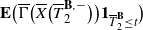${\textbf{E}}\bigl(\overline{\Gamma}\bigl(\overline{X}\bigl(\overline{T}^{{\textbf{B}},-}_{2}\bigr)\bigr)\textbf{1}_{\overline{T}^{\textbf{B}}_{2}\leq t}\bigr)$ , as required.

Reproducing the reasoning of the proof of Proposition 9, we obtain by recurrence that for any $i\in{\mathbb{N}}$ ,

\begin{align*} \lim_{{\varepsilon}\to0}{\textbf{E}}\bigl(\Gamma\bigl(X_{\varepsilon}\bigl(T^{{\textbf{B}},-}_{i,{\varepsilon}}\bigr),Y_{\varepsilon}\bigl(T^{{\textbf{B}},-}_{i,{\varepsilon}}\bigr)\bigr)\textbf{1}_{T^{\textbf{B}}_{i,{\varepsilon}}\leq t}\bigr)={\textbf{E}}\bigl(\overline{\Gamma}\bigl(\overline{X}\bigl(\overline{T}^{{\textbf{B}},-}_{i}\bigr)\bigr)\textbf{1}_{\overline{T}^{\textbf{B}}_{i}\leq t}\bigr).\end{align*}

The proof of Theorem 4 is thus complete.