2. Experimental set-up

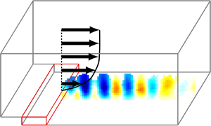
The experimental configuration is presented in figure 1. The incoming boundary layer at the separation edge (blue profile) is characterised by the free-stream velocity ($U_0$), displacement ($\delta _0$) and momentum ($\theta _0$) thickness. We denote the streamwise (direction of the free-stream), wall-normal (vertical) and spanwise (transverse) directions as $x, y, z$, respectively. The origin of the coordinate system is placed in the $x\unicode{x2013}y$ symmetry plane at the lower corner between the BFS and the floor–wall. An interchangeable insert with streamwise extent of $L_p \simeq 5$ cm marked as a red cuboid is located directly upstream of the separation edge ($-L_p \leq x \leq 0$) and extends below the level of the inlet floor channel ($0 \leq y \leq h$). To evaluate the effect of a porous material upstream of the separation edge, we consider four different insert configurations: solid impermeable insert as the reference case and three inserts made of rectified foams with $10$, $20$ and $45$ PPI (pores per inches) corresponding to $2.54$, $1.27$ and $0.56$ mm of average linear pore size, respectively.

Figure 1.

Schematic representation of an experimental set-up of BFS with $h$ as the step height. Blue profile indicates boundary layer at the separation edge characterised by the free-stream velocity $U_0$, as well as displacement ($\delta _0$) and momentum ($\theta _0$) thickness. The red volume indicates the location of the replaceable insert with length $L_{p}$. The black coordinate system defines the streamwise $(x)$, wall-normal $(y)$ and spanwise $(z)$ directions, respectively. Thin green lines mark the system that delivers dye into the recirculation zone for flow visualisations: solid and dashed lines correspond to the narrow slit and inner chamber inside the inlet floor for flow visualisations, respectively. Channel height above the porous insert upstream of the separation edge is marked as $W$.

Step height for each insert configuration was determined using a laser sheet and camera with a spatial resolution of $0.14$ mm per pixel. The laser sheet illuminated the level of the lower bounding wall upstream and downstream of the separation edge ($y=h$ at the inlet and $y=0$ at the outlet, respectively). The resulting value of $h=5.77 \pm 0.14$ mm is a compromise between ensuring the largest possible spanwise aspect ratio ($AR \approx 26$) and having a sufficient spatial resolution for the particle image velocimetry (PIV) method. The cross-section of the outlet test section downstream of the separation edge is equal to $L_y \times L_z = 10\,{\rm cm} \times 15\,{\rm cm}$. This results in an expansion ratio of $ER = L_y / W = 1.06$ (equivalent to a step-to-outlet ratio $\varGamma =h/L_y=0.058$). The small height of the step allows us to measure a large area up to $x\leq 50 h$ downstream of the separation edge. Here $W$ denotes the height of the inlet channel above the porous substrate upstream of the separation edge ($x<0$).

Permeability is the primary parameter associated with the hydrodynamics within a porous medium and describes a relationship between pressure drop across the medium and Darcy's drift velocity in the bulk of the porous medium. Typically, its value depends on the details of the geometry, such as porosity and pore diameter (Edouard et al. Reference Edouard, Lacroix, Huu and Luck2008). It also characterises the influence of the porous material on the shear flow above the porous substrate in the fluid–porous interface (Breugem et al. Reference Breugem, Boersma and Uittenbogaard2006; Suga et al. Reference Suga, Matsumura, Ashitaka, Tominaga and Kaneda2010), even at the limit of low permeability (Rosti et al. Reference Rosti, Cortelezzi and Quadrio2015). Specifically, among permeability, porosity and thickness of the porous material, the permeability was shown to be the main parameter describing the response of the shear flow to the permeable wall (Rosti et al. Reference Rosti, Cortelezzi and Quadrio2015). Finally, permeability also quantifies the effect of the porous substrate on the linear stability of the shear flow above at a given value of Reynolds number (Tilton & Cortelezzi Reference Tilton and Cortelezzi2015; Wedin et al. Reference Wedin, Cherubini and Bottaro2015). The measured permeabilities of porous inserts are $k_{1}=11.0\times 10^{-8}$ (m$^2$) for $10$ PPI, $k_1=8.9\times 10^{-8}$ (m$^2$) for $20$ PPI and $k_1=4.6\times 10^{-8}$ (m$^2$) for $45$ PPI, respectively (see Appendix A). The effective permeability pore diameter ($\sqrt {k_1}$) varies from $0.21$ mm ($45$ PPI) to $0.33$ mm ($10$ PPI) and defines the most relevant characteristic microscale within the bulk of the porous medium (Beavers & Joseph Reference Beavers and Joseph1967; James & Davis Reference James and Davis2001; Breugem, Boersma & Uittenbogaard Reference Breugem, Boersma and Uittenbogaard2005; Breugem et al. Reference Breugem, Boersma and Uittenbogaard2006), as well as in the fluid–porous interface (Ochoa-Tapia & Whitaker Reference Ochoa-Tapia and Whitaker1995; James & Davis Reference James and Davis2001).

Relative permeability normalised with channel height above the porous insert ($k_1/W^2$) is the most suitable macroscale hydrodynamical parameter of the porous medium in our geometrical configuration with low expansion ratio. Low relative permeability is equivalent to a large ratio between the hydraulic resistance of the porous insert and the hydraulic resistance of the shear flow above the porous substrate. Increasing channel height $W$ decreases relative permeability and results in a relative increase of the shear flow volume flux when compared with flux through the porous insert, in analogy to a parallel network of electrical resistors. In addition, when the effective permeability pore size ($\sqrt {k_1}$) is much lower than the height of the channel above the porous substrate ($W$), then the bulk of the porous insert becomes effectively impermeable and leads to a significant reduction of the slip velocity at the fluid–porous interface (Breugem et al. Reference Breugem, Boersma and Uittenbogaard2005).

An expansion ratio close to unity ($ER \simeq 1$) results in the low relative permeability of our inserts: $k_{1}/W^2=12.4\times 10^{-6}$ for $10$ PPI, $k_1/W^2=10.0\times 10^{-6}$ for $20$ PPI and $k_1/W^2=5.2\times 10^{-6}$ for $45$ PPI, respectively. The largest value for $10$ PPI is approximately one order of magnitude lower than the maximal relative permeability considered by Gupte & Advani (Reference Gupte and Advani1997, $k_{max}/W^2= 5.2 \times 10^{-4}$), Breugem et al. (Reference Breugem, Boersma and Uittenbogaard2006, $k_{max}/W^2= 1.9 \times 10^{-4}$), Suga & Nishio (Reference Suga and Nishio2009, $k_{max}/W^2= 8.9 \times 10^{-4}$), Suga et al. (Reference Suga, Matsumura, Ashitaka, Tominaga and Kaneda2010, $k_{max}/W^2= 9.7 \times 10^{-5}$) and Kuwata & Suga (Reference Kuwata and Suga2016, $k_{max}/W^2= 1.7 \times 10^{-4}$) to list a few. Therefore, we expect that the influence of the porous substrate will be manifested at the fluid–porous interface, rather than in the bulk of the porous inserts.

The flow visualisation system used to deliver fluorescein dye into the recirculation zone consists of an inner chamber (green dashed lines in figure 1) and narrow slit (green solid lines in figure 1) extending upstream of the replaceable insert ($x\leq -L_p$). The slit forms a narrow gap ($0 \leq y <0.5$ mm) above the level of the outlet floor that is connected with the inner chamber by spanwise-aligned row of small vertical holes ($\phi _{hole} < 0.4$ mm) shifted by $2.5$ mm along the $z$ direction. As a result, dye is gently injected from the inner chamber perpendicularly downwards towards the floor, and then distributed to the recirculation zone through the narrow slit.

The main campaign of measurements consists of two realisations for each of the four different insert configurations under consideration. These two different realisations will be distinguished by grey and black marker edges on the plots presented in the following. Each realisation consists of series of measurements, during which the free-stream velocity $U_0$ (and, thus, Reynolds number) is changed. Velocity fields were measured with a two-dimensional PIV system that consists of a Litron Nano L200-15 laser (double-headed, $532$ nm light, $1200$ mJ energy per pulse), Imager sCMOS camera ($16$-bit, $2560 \times 2160$ pix) and Davis $8.1$ Lavision software. We acquire single-frame image sequences and cross-correlate five consecutive images with temporal Gaussian weighting using $48 \times 16$ pixel interrogation windows with $4:1$ elliptical Gaussian weighting along the streamwise direction and with $50\,\%$ overlap. A rectangular interrogation window was achieved by stretching acquired images three times in the wall-normal direction using cubic interpolation. This provides us with spatial resolution of $0.59h$ and $0.19h$ along the streamwise and wall-normal direction, respectively. For each measurement we adjust acquisition frequency from $10$ to $30$ Hz (depending on $U_0$) to retain the time correlation between two consecutive snapshots. Resulting time shift between two snapshots equals approximately $0.7$ advective time units ($t_{adv} = h/U_0$). For comparison, a typical time scale of Kelvin–Helmholtz instability in our experiment was measured as $\approx 16$ advective time units. Unless otherwise stated, for all PIV measurements presented in this paper, the $1.5$-mm-thick laser sheet is aligned with the $z = 0$ plane.

Unless otherwise stated, all quantities are normalised using the step height ($h$) and free-stream velocity of the incoming boundary layer at the separation edge ($U_0$). We investigate the dynamics of BFS varying the Reynolds number, which is the main control parameter in our study defined as $Re_H=U_0 h / \nu$, with $\nu$ as the kinematic viscosity of water at room temperature.

Experiments were performed in a closed-loop water channel at Warsaw University of Technology, with the working fluid at room temperature. The experimental set-up has been already described elsewhere (Klotz, Gumowski & Wesfreid Reference Klotz, Gumowski and Wesfreid2019). The experiment described therein has been slightly modified by inserting a $5$-cm-thick block of rectified foam ($10$ PPI) upstream of the honeycombs screens. This allows us to keep background velocity fluctuations measured in the central part of free-stream below $1.7\,\%$ up to $U_0 \approx 15\,{\rm cm}\,{\rm s}^{-1}$. The bulk free-stream velocity is evaluated with calibrated PIV measurements and controlled by a large needle valve with an absolute setting precision of approximately $\Delta Re_H = \pm 5$.

The principal source of Reynolds number errors originates from the uncertainty of the determination of the free-stream velocity (${<}1.7\,\%$), which adds stochastic variation on the control parameter within each series of measurements. The second error source is related to the inaccuracy of the step height determination (${<}2.5\,\%$), which is independent of the Reynolds number and remains fixed for a given insert configuration. Therefore, it does not affect trend lines observed when the control parameter is changed other than the rescaling of abscissas of all data points in a series of measurements by a fixed constant. The third source of error originates from the limited control precision of the valve, which is less than the actual accuracy for the determination of the control parameter value. It reflects that it is substantially easier to measure the current Reynolds number than to set one specific value during the experiment. For this reason, for each series of experiments we systematically varied the Reynolds number to cover the full range of interest in our study (see e.g. Klotz et al. Reference Klotz, Goujon-Durand, Rokicki and Wesfreid2014, Reference Klotz, Gumowski and Wesfreid2019). In addition, we performed two independent series of measurements for each insert configuration. Finally, we verified that for a given flow regime, the BFS flow does not change substantially with a small variation of the control parameter.

3. Experimental results

We first present flow visualisations (streaklines) to illustrate qualitatively flow dynamics behind BFS in the early transitional regime. Fluorescein dye was excited by a point source of visible white light and released into the recirculation zone through a narrow slit at the bottom corner edge of the step geometry (see the green thin solid line for $x<-L_p$ and $y>0$ in figure 1). Instantaneous qualitative pictures of structures formed downstream of the separation edge are shown in figure 2 (top view) and figure 3 (side view). Flow visualisations are presented for a solid insert with impermeable walls (reference case, panels a,b) along with $10$ PPI porous insert configuration (panels c,d). To enhance the contrast, for each presented picture we subtract the light intensity of the background acquired for the BFS flow with no injection of the dye. The images are captured with a single Nikon D610 camera ($6016 \times 4016$ pix matrix) and a mirror inclined at $45^\circ$ to the horizontal plane. At low Reynolds number ($Re_H = 290$) both porous and solid configurations exhibit streamwise-elongated filaments of dye. This will be discussed further in § 5. Once Reynolds number is further increased to $Re_H = 510$, spanwise-coherent roller-like structures can be observed that dominate the temporal dynamics of the BFS flow. In the presence of a porous insert, these structures are shed more regularly and more frequently when compared with the reference case with solid impermeable walls. In the following part of § 3 and § 4, we characterise the unsteady dynamics of these spanwise-coherent structures formed downstream of the separation edge of BFS flow.

Figure 2.

Top view of flow visualisations for solid impermeable insert (a,b) and permeable $10$ PPI porous insert (c,d). Two Reynolds numbers are shown: $Re_H=290$ (a,c) and $Re_H=510$ (b,d).

Figure 3.

Same as figure 3 but for a side view: (a) solid, $Re_H = 290$; (b) solid, $Re_H = 510$; (c) 10 PPI, $Re_H = 290$; (d) 10 PPI, $Re_H = 510$. The recirculation bubble downstream of the separation line can be observed qualitatively on each panel.

Dovgal et al. (Reference Dovgal, Kozlov and Michalke1994) analysed the local linear stability of the local streamwise velocity profiles in streamwise-inhomogeneous BFS flow and referred to the observed structures as (local) instability waves. In the global mode framework, Marquet et al. (Reference Marquet, Sipp, Chomaz and Jacquin2008) characterised wave packet in the form of vortical structures with an alternating sign of spanwise vorticity in the vicinity of the locus of inflectional points, which are amplified and grow in space while travelling along the recirculation zone. Cantwell & Barkley (Reference Cantwell and Barkley2010) and Marais et al. (Reference Marais, Godoy-Diana, Barkley and Wesfreid2011) investigated the wake behind a cylinder, which is another example of streamwise-inhomogeneous flow configuration. They observed that the wave packet amplified within the recirculation zone in the subcritical regime consists of the street of vortices with a similar spatial structure to Bénard–von Kármán street in the supercritical regime, i.e. above the critical threshold of sustained oscillations. Finally, we also note that any measurable finite-amplitude instability wave with non-zero oscillation frequency must alter the underlying base flow inducing some surplus vorticity fluctuations $\omega _z^{\prime }$, which, in turn, manifest as vortical structures. For this reason, we refer to finite-amplitude instability waves and vortical structures interchangeably as BFS structures in the following.

Next, we evaluate quantitatively BFS flow dynamics for $Re_H\in (230,850)$ using a PIV method with measurement region covering $x/h \in (0,50h)$ and $y/h \in (0,3.0h)$. Each measurement series consists of a sequence of $2500$ snapshots covering approximately $1750$ advective time units. We investigate three porous inserts made of $10$ PPI, $20$ PPI and $45$ PPI rectified foams, along with a solid Plexiglas insert as the reference case. For each configuration, two independent realisations are taken to assess the robustness of the analysis and to evaluate possible sensitivity to external noise in the installation. Flow visualisations in figures 2 and 3 and PIV measurements presented in the following were acquired in different runs.

The instantaneous spatial distribution of streamwise ($u/U_0$) and wall-normal ($v/U_0$) velocity components measured with the PIV technique are presented in figures 4 and 5, respectively. The spatial distribution of instantaneous vorticity fluctuations (the difference between instantaneous and time-averaged vorticity fields denoted as $\omega _z^{\prime }$) is illustrated in figure 6. Each column corresponds to a single Reynolds number, $Re_H \in (290,410,510)$ from left to right. Each of the presented fields is extracted from a different series of measurements and variations between the actual Reynolds numbers resulting from an absolute setting precision of the controlling valve is approximately $\Delta Re_H = \pm 5$. Rows represent solid Plexiglas, $45$ PPI and $10$ PPI porous insert configurations, from top to bottom. In addition, on each panel we superpose time-averaged recirculation zones (dashed magenta curve) and the locus of inflectional points of time-averaged streamwise velocity profiles (dashed magenta curve). Specifically, the regions of reversed flow downstream and below the separation edge are observed for all insert configurations.

Figure 4.

Instantaneous streamwise velocity component ($u/U_0$) measured with a two-dimensional PIV technique for solid (a–c), $45$ PPI (d–f) and $10$ PPI (g–i) insert configurations, from top to bottom. The first (a,d,g), second (b,e,h) and third (c,f,i) columns correspond to $Re_H = 290$, $Re_H = 410$ and $Re_H = 510$, from left to right. In each panel, the locus of the inflectional point in the shear-layer profiles (magenta dashed line) and recirculation zone (magenta dotted line) are superposed.

Figure 5.

Same as in figure 4 but for instantaneous wall-normal velocity component ($v/U_0$): for solid (a–c), 45 PPI (d–f) and 10 PPI (g–i) insert configurations, from top to bottom. The first (a,d,g), second (b,e,h) and third (c,f,i) columns correspond to $Re_H = 290$, $Re_H = 410$ and $Re_H = 510$, from left to right.

Figure 6.

Same as in figure 4 but for instantaneous spanwise vorticity fluctuations ($\omega ^{\prime }_z h/U_0$) defined as the difference between instantaneous and time-averaged spanwise vorticity fields: for solid (a–c), 45 PPI (d–f) and 10 PPI (g–i) insert configurations, from top to bottom. The first (a,d,g), second (b,e,h) and third (c,f,i) columns correspond to $Re_H = 290$, $Re_H = 410$ and $Re_H = 510$, from left to right.

Laminar featureless flow at low Reynolds number is presented in the left columns of figures 4–6. The central columns illustrate the flow at sufficiently high $Re_H$, above which a spatially periodic pattern of BFS structures can be observed. The right columns represent the flow at a further increased Reynolds number, at which distinct spatially periodic patterns are preserved. These BFS structures manifest by waviness of the streamwise velocity component (figure 4), street of coherent regions of vertical velocity with alternating signs (figure 5) and street of alternating vorticity fluctuations along the streamwise direction (figure 6). A comparison between left and central columns indicates a bifurcation leading to the formation of the finite-amplitude structures downstream of the separation edge for sufficiently large Reynolds numbers. The quantitative analysis of this bifurcation, which includes the determination of the thresholds using the Landau model, are presented in § 4.

Our observation that spatial periodic structure is most pronounced on the vertical component $v/U_0$ agrees with former numerical results (see e.g. Blackburn et al. Reference Blackburn, Barkley and Sherwin2008; Marquet & Sipp Reference Marquet and Sipp2012; Boujo & Gallaire Reference Boujo and Gallaire2015). In addition, the structure of the perturbation consists of elliptical shapes with major axes aligned with the vertical and horizontal directions, in agreement with Blackburn et al. (Reference Blackburn, Barkley and Sherwin2008). Moreover, Cantwell & Barkley (Reference Cantwell and Barkley2010) and Marais et al. (Reference Marais, Godoy-Diana, Barkley and Wesfreid2011) demonstrated that cross-flow (wall-normal) velocity component is a good representation of vortical structures observed both below and above the critical threshold of the Bénard–von Kármán street in the wake behind a cylinder. For these reasons in the rest of the paper we concentrate our analysis on $v/U_0$, in analogy with the analysis of a cylinder wake (Marais et al. Reference Marais, Godoy-Diana, Barkley and Wesfreid2011) or jet in a cross-flow (Megerian et al. Reference Megerian, Davitian, Alves and Karagozian2007; Klotz et al. Reference Klotz, Gumowski and Wesfreid2019).

4. Spectral analysis

For each spatial location ($x,y$) we perform temporal fast Fourier transform (FFT) analysis of the $v(t)/ U_0$ signal. The long sequence of measurements is divided into nine subsequences without overlap and with duration of ${\approx }200$ advective time units each. This covers more than 12 full periods of Kelvin–Helmholtz instability. All subsequences are ensemble-averaged to obtain the final spatial distribution of amplitude $A_{FFT}/U_0$ for each frequency in the spectrum. First, we extract spatio-spectral diagrams at wall-normal locations, at which standard deviation in time of $v/U_0$ reaches the maximum. Dependence of the Strouhal number ($St_H= (f h)/(U_0)$) on streamwise location is shown in figure 7. Vertical lines can be distinguished on these diagrams, which demonstrates the existence of global coherent spectral modes with well-defined characteristic Strouhal number that prevails along the streamwise direction in the separated shear layer formed behind the BFS. Their spectral amplitudes reach the maximal value at some finite distance from the separation edge ($15h-25h$, depending on $Re_H$ and porous insert configuration) and subsequently decay. This is in analogy with the global mode evolution observed in the wake of a cylinder (Goujon-Durand, Jenffer & Wesfreid Reference Goujon-Durand, Jenffer and Wesfreid1994; Wesfreid, Goujon-Durand & Zielinska Reference Wesfreid, Goujon-Durand and Zielinska1996), three-dimensional bluff bodies (Ormières & Provansal Reference Ormières and Provansal1999; Klotz et al. Reference Klotz, Goujon-Durand, Rokicki and Wesfreid2014), jet in a cross-flow (Klotz et al. Reference Klotz, Gumowski and Wesfreid2019; Chauvat et al. Reference Chauvat, Peplinski, Henningson and Hanifi2020) or hot free jet (Coenen et al. Reference Coenen, Lesshafft, Garnaud and Sevilla2017). Our observations are also in agreement with Blackburn et al. (Reference Blackburn, Barkley and Sherwin2008) who reported that non-trivial dynamics of the separated shear flow extends further downstream of the step, and is not solely determined by the initial roll-up of the shear layer at the separation edge.

Figure 7.

Spatio-spectral diagrams with normalised frequency ($St_H$) on the horizontal and streamwise coordinate ($x/h$) on the vertical axis for different $Re_H$: (a–f) solid, (g–l) $45$ PPI and (m–r) $10$ PPI porous configurations, from top to bottom; (a) $Re_H = 295$; (b) $Re_H = 365$; (c) $Re_H = 405$; (d) $Re_H = 515$; (e) $Re_H = 575$; ( f) $Re_H = 675$; (g) $Re_H = 285$; (h) $Re_H = 365$; (i) $Re_H = 410$; ( j) $Re_H = 505$; (k) $Re_H = 580$; (l) $Re_H = 685$; (m) $Re_H = 290$; (n) $Re_H = 365$; (o) $Re_H = 405$; ( p) $Re_H = 510$; (q) $Re_H = 570$; (r) ${Re_H = 700}$.

Next, we average spatio-spectral diagrams over the streamwise direction $x$. Selected results for solid, $45$ PPI, $20$ PPI and $10$ PPI insert configurations are shown in figure 8(a–d), from left to right. For the solid configuration, two characteristic Strouhal numbers can be distinguished: at low Reynolds numbers ($Re_H=325$ and $Re_H=365$), no peak at $\approx 0.055$ can be distinguished and only a peak at $St_{H} \approx 0.035$ is present. For $Re_H=460$, a new weak peak emerges at $St_{H} \approx 0.055$ and eventually it becomes the main peak in the spectrum for sufficiently large Reynolds number ($Re_H=675$). For the $45$ PPI insert configuration, we observe analogical spectral shift but at lower Reynolds number when compared with solid insert configuration. For $20$ PPI, a weak signature of lower characteristic Strouhal number can be distinguished only at the lowest $Re_H$, and for the $10$ PPI configuration, a dominant peak occurs at $\approx 0.055$ for the entire range of Reynolds numbers under consideration.

Figure 8.

Selected spectra resulting from averaging spatio-spectral diagrams along the streamwise direction: (a) solid boundary configuration; (b) $45$ PPI rectified foam configuration; (c) $20$ PPI rectified foam configuration; (d) $10$ PPI rectified foam configuration. The $Re_H$ values are shown in corresponding legends on each panel.

4.1. Characteristic Strouhal numbers and frequency cross-over

For each insert configuration, Reynolds number and realisation, we determine a global dominant spectral peak (with positive frequency) and associated global peak of FFT amplitude ($A_{FFT}$) within the entire area of measurements. In contrast to results shown in figure 8, the data in figure 9 do not include averaging along the streamwise direction. In figure 9 we present the dependence of dominant $St_H$ on $Re_H$ for four insert configurations: solid insert (orange triangles), $45$ PPI insert (violet squares), $20$ PPI insert (green reversed triangles) and $10$ PPI insert (blue circles). For each insert configuration different edge colours of the markers are used to distinguish between two independent series of measurements.

Figure 9.

Dominant normalised frequencies $St_H=f h/U_0$ for each realisation and each configuration as a function of the control parameter $Re_H$. Light blue and dark red semi-transparent areas indicate two main spectral regions, in which data points are grouped. Orange triangles, violet squares, reversed green triangles and blue circles correspond to solid, $45$ PPI, $20$ PPI and $10$ PPI insert configurations, respectively. Black and grey edges of the markers indicate two different series of measurements for each porous insert configuration. Solid vertical lines in corresponding colours mark the frequency cross-over from lower to higher frequencies.

All measurement points can be grouped into two distinct spectral regions marked by dark-red ($0.048< St_{H2}<0.070$) and light-blue ($0.020< St_{H1} <0.042$) shaded areas. We ensemble-averaged all data points within each of these two spectral regions to obtain two characteristic central frequencies, which results in $St_{H1} = 0.033$ and $St_{H2} = 0.058$. In the following, we refer to these characteristic frequencies and corresponding spectral amplitudes as spectral mode 1 and 2, respectively. Once the Reynolds number is increased, a cross-over between dominant Strouhal numbers and corresponding spectral modes can be observed. Estimated Reynolds numbers, at which this cross-over occurs, are marked by thick solid vertical lines in the same colours as the corresponding markers. Increasing permeability of the insert promotes frequency cross-over to occur at lower values of $Re_H$. Apart from the switch of dominating frequency, the characteristic Strouhal numbers do not depend on Reynolds number: despite some intrinsic scatter of the measured frequencies, the results fall on one of two horizontal trend lines for each realisation. In fact, some scatter is expected due to large potential for perturbation amplification in BFS (e.g. Blackburn et al. Reference Blackburn, Barkley and Sherwin2008; Marquet et al. Reference Marquet, Sipp, Chomaz and Jacquin2008; Sipp et al. Reference Sipp, Marquet, Meliga and Barbagallo2010; Dergham et al. Reference Dergham, Sipp and Robinet2013; Boujo & Gallaire Reference Boujo and Gallaire2015).

4.2. Bifurcation diagram of spectral amplitudes

In figure 10 we show a bifurcation diagram illustrating a dependence of squared amplitude of dominant FFT mode ($E=A_{FFT}^2 / U_{0}^2$ for the mode with positive frequency) on Reynolds number $Re_H$. All markers, colours and solid vertical lines are the same as in figure 9. Each subsequent configuration is shifted upwards by $0.0012$ to increase readability of the plot and zero reference levels are marked by horizontal dotted lines in corresponding colours.

Figure 10.

Dependence of the dominant spectral mode amplitude on control parameter $Re_H$ for a solid insert (orange triangles), $45$ PPI (violet squares), $20$ PPI (reversed green triangles) and $10$ PPI (blue circles) porous inserts. Solid vertical lines indicate the frequency cross-over from spectral mode 1 to spectral mode 2. Linear increase of the squared amplitude of the dominant spectral mode is marked by a black dashed line for all three porous inserts. Horizontal dashed lines in corresponding colours indicate energy saturation of the dominant mode for higher Reynolds numbers. Series of measurements for each subsequent configuration is shifted upwards by $0.0012$ to increase readability of the plot and zero reference levels are marked by horizontal dotted lines in corresponding colours.

For all four insert configurations, the squared amplitude of the dominant mode reaches fully saturated value at sufficiently large Reynolds number. This is marked by horizontal dashed lines in corresponding colours. Similar saturation of the dominant frequency has been observed for wake behind a cylinder (Zielinska et al. Reference Zielinska, Goujon-Durand, Dušek and Wesfreid1997; Mantič-Lugo et al. Reference Mantič-Lugo, Arratia and Gallaire2014).

However, the dependence of $E(Re_H)$ prior to the fully saturated regime is different for a solid insert when compared with the three porous configurations. Specifically, for $10$ PPI, $20$ PPI and $45$ PPI inserts, $E$ is close to zero at low enough Reynolds numbers (blue circles, green triangles and violet squares in figure 10). Once the Reynolds number exceeds some critical value $Re_c$, the squared amplitude of dominant mode ($E$) starts to grow proportionally to the distance from the threshold, as indicated by black dashed lines. This behaviour of the order parameter agrees with the Landau model and indicates the occurrence of Hopf bifurcation at $Re_c$. We determined threshold values for each porous insert by interpolating linear growth of $E(Re_H)$ to zero. This results in $Re_{c}\approx 350$ for $10$ PPI, $Re_{c}\approx 420$ for $20$ PPI and $Re_{c} \approx 450$ for $45$ PPI. In contrast, for the solid insert (orange triangles in figure 10), the squared amplitude of the dominant mode grows gradually with no visible change of growth trend once the Reynolds number is increased.

Furthermore, for all porous insert configurations the frequency cross-over (blue, green and violet solid vertical lines in figure 10) occurs prior to the threshold $Re_{c}$ associated with Hopf bifurcation. This demonstrates that entire growth of $E$ presented on this bifurcation diagram can be attributed to the dominating spectral mode 2. In contrast, for a solid insert the frequency cross-over is observed only when $E$ reaches approximately half of its final saturated value showing that both spectral modes 1 and 2 contribute to the growth of $E$ presented in figure 10.

According to the Landau model, the amplitude of the oscillations is zero below the critical threshold and starts to grow when the control parameter exceeds the critical Reynolds number, with its squared value proportional to the distance from the critical threshold (i.e. $(A_{FFT})^2 \sim (Re-Re_C)$). This transition is due to Hopf bifurcation associated with a linear instability of the base flow with non-zero frequency at the critical threshold. The exponential growth of instability for finite values of $Re-Re_C$ is reduced to zero through a nonlinear cubic term in the Landau equation, which results in finite-amplitude oscillations (i.e. limit cycle). In our experiment, the amplitude $A_{FFT}$ of dominating spectral mode 2 follows the prediction of the Landau model for all porous inserts. In contrast, our experimental data do not clearly support the existence of a supercritical limit cycle for the solid insert configuration. Our observations thus support the suggestion of Marquet et al. (Reference Marquet, Lombardi, Chomaz, Sipp and Jacquin2009) who postulated that the recirculation zone behind the step can be an optimal location for a passive control device.

4.3. Spatial support for spectral modes: Hilbert transform

In figures 11 and 12, we illustrate the spatial distribution of envelope amplitudes associated with spectral modes 1 and 2, respectively. The envelopes are calculated using Hilbert transform for spectral ranges marked by light-blue and dark-red semi-transparent areas in figure 9. Difference between the spatial distribution of envelopes 2 and 1 is illustrated in figure 13: blue and red colours represent the regions dominated by spectral modes 1 and mode 2, respectively. Columns in figures 11–13 correspond to $Re_H \in (290, 410, 510)$ with $\Delta Re_H = \pm 5$, from left to right. Rows are associated with solid, $45$ PPI and $10$ PPI porous insert configurations, from top to bottom.

Figure 11.

Time-averaged spatial envelope reconstructed using Hilbert transform on the spectral range corresponding to mode 1. Solid insert, $45$ PPI and $10$ PPI porous insert configurations are presented in (a–c), (d–f) and (g–i), from top to bottom. Panels (a,d,g), (b,e,h) and (c,f,i) correspond to $Re_H \in (290,410,510)$, from left to right. On each field, magenta dotted and dashed curves are superposed to mark the time-averaged recirculation zone and locus of inflection points of time-averaged streamwise velocity profiles. Compare with figures 4–6.

Figure 12.

Same as figure 11 but for spectral range corresponding to mode 2: solid insert, 45 PPI and 10 PPI porous insert configurations are presented in rows (a–c), (d–f) and (g–i), from top to bottom. Columns (a,d,g), (b,e,h) and (c,f,i) correspond to $Re_H \in (290, 410, 510)$, from left to right.

Figure 13.

Difference between spatial support of spectral mode 2 and spectral mode 1 envelopes: solid insert, 45 PPI and 10 PPI porous insert configurations are presented in rows (a–c), (d–f) and (g–i), from top to bottom. Columns (a,d,g), (b,e,h) and (c, f,i) correspond to $Re_H \in (290, 410, 510)$, from left to right.

For the solid insert configuration, the average spatial intensity of envelope 1 is larger than envelope 2, in agreement with figures 9 and 10. The first row in figures 11 and 13 indicate that this dominance is mostly pronounced downstream the reattachment of the separated shear layer, with maximal value located slightly above the separation edge ($y>h$). However, envelope 2 can locally dominate in the vicinity of the recirculation zone marked as dotted magenta curves.

Spatial envelopes for $45$ PPI are shown in the second row of figures 11–13. Below the threshold of limit cycle oscillations ($Re_H < Re_c\approx 450$ for $45$ PPI), spatial distribution of the envelope difference is similar to the solid insert configuration with the dominance of envelope 1 downstream of the reattachment line, as illustrated in figure 13(d,e) (compare with figure 13(a–c) for the solid insert configuration). However, for $Re_H=510$, envelope 2 starts dominating downstream of the reattachment (figure 13f). Similar transition of the spatial envelope structure with increasing $Re_H$ is also observed for $10$ PPI in the third row of figure 13. Below the critical threshold ($Re_H < Re_c\approx 350$ for $10$ PPI), envelope 1 is dominating downstream (figure 13g), whereas above this threshold the intensity of envelope 2 overtakes in the entire region of measurements with a maximal value slightly above the locus of inflectional points marked by a dashed magenta curve (figure 13h,i).

To further characterise the streamwise dependence of both envelopes, we calculate their mean value along the wall-normal direction for each streamwise location $x/h$. The results are presented in figure 14: solid, $45$ PPI, $20$ PPI and $10$ PPI porous insert configurations are shown in the rows from top to bottom; left and right columns represent envelopes 1 and 2, respectively. On each panel, we present the streamwise envelope intensity for several selected values of $Re_H$, the values of which are listed in legends on the right.

Figure 14.

Streamwise dependence of amplitudes of envelope 1 (a,c,e,g) and envelope 2 (b,d,f,h). Panels (a,b), (c,d), (e,f) and (g,h) correspond to solid, $45$ PPI, $20$ PPI and $10$ PPI porous inserts, from top to bottom. The $Re_H$ values for each insert configuration are indicated in legends. Each point at a given $x/h$ results from averaging envelopes shown in figures 11 and 12 in time and along wall-normal direction. All presented curves are smoothed along the $x$ direction between three neighbouring points.

For solid insert configuration, both envelopes reach a global maximum at $x/h \approx 20$ and their dependence along the streamwise direction is similar (figure 14a,b). In addition, the spatial peak of envelope 1 is larger than that of envelope 2 up to $Re_H = 675$ (blue circles in figure 14a,b), in agreement with the frequency cross-over shown in figure 9. After initial streamwise growth, the amplitude of envelope 1 tends to reach a constant equilibrium value further downstream. In addition, the global peak of envelope 1 for porous inserts (figure 14c,e,g) does not change significantly when compared with the solid insert configuration (figure 14a).

In contrast, porous inserts heavily influence BFS structures characterised by the spectral range of mode 2. Envelope 2 for all porous inserts is characterised by non-monotonic streamwise evolution, reaching their maximal value at some finite distance from the step and subsequently decaying further downstream. In addition, the streamwise location of the global peak shifts upstream with increasing $Re_H$, in analogy with Mantič-Lugo & Gallaire (Reference Mantič-Lugo and Gallaire2016a). This streamwise evolution of envelope 2 for porous inserts is similar to the spectral mode evolution shown in figure 7.

The different streamwise evolutions of envelopes 1 and 2, combined with their different spatial support observed for porous inserts, indicate that the dynamics characterised by spectral range 2 is associated with the mixing-layer region in the vicinity of the recirculation zone. In contrast, envelope 1 corresponds to the dynamics of the boundary-layer region downstream of the reattachment of the separated shear layer.

4.4. Origin of dominant spectral modes

Characteristic frequencies of mode 1 and mode 2 are nearly commensurate. We note that for solid insert configuration at low $Re_H$ only mode 1 can be observed (see red curve for $Re_H=325$ in figure 8a). Significant peak corresponding to mode 2 can be detected in the spectrum only at larger values of $Re_H$ (e.g. green curve for $Re_H=460$ in figure 8a). This shows that mode 1 is not a subharmonic of mode 2. Therefore, BFS dynamics is different from subharmonic resonance in free mixing layers, for which first subharmonic was least-stable secondary instability to the equilibrated train of primary vortices related to fundamental frequency.

Similarly, for $10$ PPI insert configuration, mode 2 fully dominates the spectrum and very weak/no spectral signature of mode 1 can be distinguished (figure 8d). Moreover, mode 2 grows faster along the streamwise direction and reaches maximum closer to the separation edge when compared to mode 1 (figures 13 and 14), which indicates that mode 2 is not a higher harmonic of mode 1. This demonstrates that modes 1 and mode 2 are two separate spectral modes with two different characteristic frequencies. In this context, Boujo & Gallaire (Reference Boujo and Gallaire2015) observed a transition of linear harmonic BFS response from one to two dominant frequencies once the expansion ratio is decreased from $ER=2$ to $ER=1.4$. Our value of $ER=1.06$ is below the estimated transition range reported by Boujo & Gallaire (Reference Boujo and Gallaire2015) and thus a two-peak response can be expected.

To better assess characteristic frequencies for each mode, we acquired few additional series of measurements for solid and $10$ PPI porous inserts. We compute the spectra using a similar method as described in the first paragraph of § 4 but with 50 % longer time series for each sub-sequence. Then, we ensemble-averaged the results for all three long series of measurements. This allowed us to increase spectral resolution by 50 % when compared to the data presented in figure 8. Resulting spectra are presented in figure 15 with Reynolds numbers listed in the legends. This extended analysis confirms that at low $Re_H$ BFS dynamics with solid insert is dominated by low-frequency mode 1 (red stars in figure 15a). As $Re_H$ is increased the amplitude of mode 2 increases and eventually becomes dominant. Characteristic frequency of mode 1 remains constant as illustrated by red vertical solid line, with additional red dashed lines indicating the spectral resolution of FFT transform. Spectral range allowed for the first higher harmonic of mode 1 is marked in figure 15(a) as black vertical dashed line with black dotted vertical lines indicating the spectral accuracy for higher harmonic (twice the spectral resolution). Peaks of mode 2 (black crosses in figure 15a) lie outside the spectral range of the higher harmonic of mode 1 for all measured spectra, which confirms that mode 2 is not a higher harmonic of mode 1. Furthermore, on both panels in figure 15, the spectral range associated with near-zero frequency modes is relatively flat with no significant and robust peaks in the vicinity of zero frequency for investigated $Re_H$ range and for our spectral resolution.

Figure 15.

Spectra averaged along the streamwise direction for solid (a) and $10$ PPI porous inserts (b). Each spectrum is ensemble-averaged over three different long series of measurements. This results in 50 % better resolution in frequency when compared with figure 8 and with higher signal-to-noise ratio at lower frequencies. Red solid and black dashed vertical lines illustrate the characteristic frequency of spectral mode 1 and its higher harmonic, respectively.

One can distinguish at least two more characteristic length scales in BFS flow different from step height $h$, such as momentum thickness ($\theta _{0}$) of incoming boundary layer at the separation edge or displacement thickness ($\delta _{r}$) close to the streamwise location where separated shear layer re-attaches. Momentum thickness is conventionally used in the context of free mixing shear layers (e.g. Ho & Huerre Reference Ho and Huerre1984), whereas displacement thickness is more frequently applied in boundary layer flow (e.g. Obremski et al. Reference Obremski, Morkovin, Landahl, Wazzan and Okamura1969; Ehrenstein & Gallaire Reference Ehrenstein and Gallaire2005; Alizard, Cherubini & Robinet Reference Alizard, Cherubini and Robinet2009; Monokrousos et al. Reference Monokrousos, Åkervik, Brandt and Henningson2010; Wedin et al. Reference Wedin, Cherubini and Bottaro2015). In figure 16(a,b) we present characteristic frequencies of both spectral modes normalised with $\theta _{0}$ and $\langle \delta _{r}\rangle$, respectively. $\langle \delta _{r}\rangle$ is calculated from streamwise velocity profile averaged along the streamwise direction starting from re-attachment ($x_r$) and spanning $2h$ downstream ($x_r^{\prime }=x_r+2h$). Variation of both $St_{\theta }(Re_H)$ and $St_{\delta }(Re_H)$ illustrated in figure 16(a,b) is more pronounced than the variation of $St_{h}(Re_H)$ presented in figure 9. This shows that for a given value of $ER$, step height $h$ is the most appropriate length scale for BFS flow. However, independently of the selected characteristic length scale, all measured points group onto two distinct branches associated either with mode 1 (lower branch at the bottom of figures 9 and 16) or mode 2 (upper branch at the top of figures 9 and 16).

Figure 16.

Strouhal numbers computed using different characteristic length scales: (a) momentum thickness at the separation edge, $\theta _{0}$; (b) displacement thickness downstream of the reattachment, $\langle \delta _{r} \rangle$. Compared with figure 9 where step height $h$ is used as the length scale. Horizontal red lines in (a) correspond to the most amplified frequency calculated using spatial local linear theory for the mixing layer (solid, Michalke Reference Michalke1965; Freymuth Reference Freymuth1966; dashed, Ho & Huerre Reference Ho and Huerre1984). Horizontal non-red solid lines in (a) represent reported values for roll-up of the shear layer for BFS (Eaton & Johnston Reference Eaton and Johnston1982; Chun & Sung Reference Chun and Sung1996; Dovgal & Sorokin Reference Dovgal and Sorokin2004). Dashed curves in (b) correspond to the most amplified frequency of the Falkner–Skan family of boundary layers with Hartree parameter $\beta =-0.198$ (Obremski et al. Reference Obremski, Morkovin, Landahl, Wazzan and Okamura1969 in red; Wazzan, Taghavi & Pafford Reference Wazzan, Taghavi and Pafford1986 in cyan) and $\beta =-0.140$ (Obremski et al. Reference Obremski, Morkovin, Landahl, Wazzan and Okamura1969 in green). Correlation proposed by Xu et al. (Reference Xu, Bai, Qiao and Zhang2019) is also superposed as magenta curve.

Local spatial stability analysis (Michalke Reference Michalke1965) along with experimental measurements in free mixing layer (Freymuth Reference Freymuth1966) indicated that $St_{\theta }=0.017$ is the most unstable frequency amplified through inviscid Kelvin–Helmholtz instability due to inflectional point in the time-averaged streamwise velocity profile. Ho & Huerre (Reference Ho and Huerre1984) reported about similar value of $St_{\theta }=0.016$ (note that here we transform their results using free-stream velocity $U_0$ as the velocity scale). Both values are marked as red horizontal lines in figure 16(a). The largest $St_{\theta }$ were measured at the frequency cross-over from mode 1 to mode 2, with maximal values of approximately $0.016$, $0.015$, and $0.014$ for $10$ PPI, $20$ PPI, and $45$ PPI, respectively. These values are in good agreement with linear stability prediction for free mixing shear layer, demonstrating that the maximal allowed value of $St_{\theta }$ on the upper branch is bounded from above by the most unstable frequency of the shear layer at the separation edge. In addition, $St_{\theta }$ on the upper branch decreases once the Reynolds number $Re_H$ is increased, in analogy to the trend reported by Michalke & Hermann (Reference Michalke and Hermann1982) for free jet. Our results on $St_{\theta }$ for the largest Reynolds number under investigation ($Re_H\approx 900$) compare well with the values reported by Eaton & Johnston (Reference Eaton and Johnston1982), Chun & Sung (Reference Chun and Sung1996) and Dovgal & Sorokin (Reference Dovgal and Sorokin2004) marked as horizontal non-red solid lines on the right of figure 16(a). Overall agreement between measured frequencies on upper branch frequencies and results reported for free mixing shear layer and BFS demonstrates that the upper branch associated with mode 2 corresponds to Kelvin–Helmholtz instability.

This is further demonstrated in figure 17(a), on which we plot time-averaged velocity profiles measured for all Reynolds numbers and all considered inserts (approximately 300 independent series of measurements). As already mentioned in the introduction, the dynamics of the perturbation at the separation edge in BFS shares similarity with the free-mixing shear layer. Therefore, the wall-normal coordinate is normalised with the momentum thickness of the boundary layer at the separation edge $\theta _0$. In addition, for each measured velocity profile the wall-normal locations were shifted by $\Delta y$, such that $u(y_s) = 0.5U_0$ for $y_s =y-\Delta y=0$. We also superpose classical hyperbolic-tangent mixing layer velocity profile ($0.5(1+\tanh (y_s/2\theta _0)$) illustrated by a thick dashed magenta curve. All the measured streamwise velocity profiles collapse to a single curve that compares well with a hyperbolic tangent. This demonstrates that immediately downstream of the separation edge, BFS dynamics can be considered as analogical to the free-mixing shear layer and dominated by Kelvin–Helmholtz instability, as already mentioned in the introduction.

Figure 17.

Time-averaged streamwise velocity profiles measured: (a) immediately downstream of the separation edge; (b) at re-attachment of separated boundary layer, $x=x_r$; (c) $2h$ downstream of the re-attachment, at $x=x_r^{\prime }=x_r+2h$; (d) streamwise-averaged for $x \in (x_r, x_r^{\prime })$. Wall-normal coordinate $y$ is normalised with momentum (a) and displacement (b–d) thickness computed separately for each presented location. Magenta curve in (a) represents free mixing shear layer solution ($u(y)=0.5+0.5\tanh (y_s/2\theta _0)$). Dashed curves in (b–d) represent velocity profiles of Falkner–Skan boundary layer flow with Hartree parameter: $\beta =-0.198$ (at the re-attachment of boundary layer; in red), $\beta =-0.140$ ($2h$ downstream the re-attachment; in green). In (b–d) velocity profiles with $Re_H$ below the threshold of frequency cross-over are shown.

In figure 16(b) we present characteristic frequency normalised with displacement thickness in the vicinity of the re-attachment of separated shear layer as a function of $Re_H$. The lower branch associated with mode 1 covers the spectral range of $St_{\delta }\in (0.02-0.06)$. We compare lower branch frequencies to the results derived from local linear stability analysis of Falkner–Skan family of boundary layer profiles, with Hartree parameter $\beta$ that quantifies the intensity of the adverse pressure gradient. Specifically, we consider $\beta =-0.198$ and $\beta =-0.140$.

First, we demonstrate the universal character of the streamwise velocity profiles in the vicinity of the reattachment of the separated shear layer. In figure 17(b–d) we select velocity profiles with $Re_H$ below the threshold of frequency cross-over for which mode 1 is dominating. On each panel, we overlap all selected velocity profiles without distinguishing insert configuration, Reynolds number or realisation. Specifically, we consider streamwise location, at which separated shear layer reattaches ($x_r$ in figure 17b), streamwise location located two steps heights downstream of the reattachment ($x_r^{\prime }=x_r+2h$ in figure 17c) and velocity profile averaged along the streamwise direction for $x\in (x_r,x_r^{\prime })$ (figure 17d). For reference, we also superpose Falkner–Skan velocity profiles for $\beta =-0.198$ and $\beta =-0.140$ that represent local velocity profile at the reattachment (red dashed curve) and $2h$ downstream of the separation line (green dashed curve), respectively. The wall-normal coordinate $y$ is normalised by displacement thickness at the reattachment ($\delta _{r}$ in figure 17b), displacement thickness $2h$ downstream of the reattachment ($\delta _{r^{\prime }}$ in figure 17c), and displacement thickness of the velocity profile averaged along the streamwise direction $x\in (x_r,x_r^{\prime })$ ($\langle \delta _{r}\rangle$ in figure 17d). One can observe that the measured velocity profiles at $x_r$ and $x_r^{\prime }$ compare well with Falkner–Skan velocity profiles with $\beta =-0.198$ and $\beta =-0.140$, respectively.

The local intensity of the adverse streamwise pressure gradient associated with specific Hartree parameter $\beta$ is a value that is required at a given streamwise location to preserve self-similarity of the Falkner–Skan solution along the streamwise direction. If, at any location, this value is lower than required, then the local velocity profile will relax further downstream towards a solution that is closer to the zero-pressure equilibrated boundary layer (i.e. towards a solution with $\beta$ closer to zero). As already mentioned in the introduction, BFS flow is not self-similar along the streamwise direction and it represents spatial relaxation of free-mixing layer flow into an equilibrated boundary layer profile further downstream. This implies that the local intensity of the adverse pressure gradient is lower than required by the Falkner–Skan solution to preserve streamwise self-similarity. Furthermore, the agreement between one specific self-similar Falkner–Skan solution and measured velocity profiles occurs only locally at one specific streamwise location.

In figure 17(b–d) we established that velocity profiles in the vicinity of re-attachment can be locally spanned between Falkner–Skan solutions for $\beta =-0.198$ and $\beta =-0.140$. Now we compare the measured spectral range of the lower branch with the most amplified frequencies of these two Falkner–Skan boundary layers. Obremski et al. (Reference Obremski, Morkovin, Landahl, Wazzan and Okamura1969) studied local linear stability of the Falkner–Skan solution and presented in their figure 10(m,n) the dependency of the most amplified frequency of the Tollmien–Schlichting wave on the Reynolds number based on displacement thickness. However, they did not state $f_{TS}(Re_{\delta })$ dependency explicitly. The cups of iso-contours shown in figure 10(m,n) from Obremski et al. (Reference Obremski, Morkovin, Landahl, Wazzan and Okamura1969) fall on the straight line on a log–log scale. Therefore, we infer the coordinates of these cusps and fit a power-law dependence to estimate the missing $f_{TS}(Re_{\delta })$ dependency. Finally, we substitute the dependence of local values of $Re_{\delta }(Re_H)$ measured in our experiments and compare with our spectral results.

The resulting spectral range for the most amplified frequencies of Tollmien–Schlichting waves is marked in figure 16(b) and spans from $\beta =-0.198$ (red dotted curve) to $\beta =-0.140$ (green dotted curve). We also superposed results reported by Wazzan et al. (Reference Wazzan, Taghavi and Pafford1986, cyan curve) and Xu et al. (Reference Xu, Bai, Qiao and Zhang2019, magenta curve). Measured Strouhal numbers of the lower branch (mode 1) are contained within the spectral range bounded above by the curves associated with $\beta =-0.198$ (Obremski et al. Reference Obremski, Morkovin, Landahl, Wazzan and Okamura1969; Wazzan et al. Reference Wazzan, Taghavi and Pafford1986), and bounded below by the curve related to $\beta =-0.140$ (Obremski et al. Reference Obremski, Morkovin, Landahl, Wazzan and Okamura1969) and correlation reported by Xu et al. (Reference Xu, Bai, Qiao and Zhang2019). Moreover, the largest measured values of $St_{\delta }$ on a lower branch are in relatively good agreement with the most amplified frequency for $\beta =-0.198$. The streamwise velocity profile at this location is expected to be the least stable among all velocity profiles within the Falkner–Skan family of boundary layers (Obremski et al. Reference Obremski, Morkovin, Landahl, Wazzan and Okamura1969). This indicates that the mode 1 lower branch is related to the Tollmien–Schlichting instability.

We note that in contrast to the well-defined reattachment location $x_r$, the downstream limit $x_r^{\prime }$ for streamwise averaging has been selected arbitrarily. For any location selected further downstream than $x_r^{\prime }$, the intensity of adverse pressure gradient would decrease (i.e. $\beta$ closer to zero) and lower bound limit for $St_{\delta }$ (green dotted curve in figure 16b) would shift closer to abscissa.

Regarding the relation between local and global stability analysis, Boujo & Gallaire (Reference Boujo and Gallaire2015) investigated BFS flow with solid impermeable walls and $ER=2.0$. They reported that the most amplified frequency response of BFS structures calculated using global stability analysis (i.e. incorporate streamwise eigendirection directly into eigenfunctions) agrees well with the most amplified frequency derived by integration along the streamwise direction of local amplification rates calculated independently for each streamwise location using local stability analysis (i.e. under the additional assumption of streamwise homogeneity at each streamwise location). This indicates that local stability analysis can provide meaningful criteria for the prediction of the most amplified perturbation frequency.

5. Measurements in cross-stream planes

Flow visualisations presented in figure 2(a,c) reveal weak streamwise-elongated structures, with spanwise wavelength that differs from the value reported by Barkley et al. (Reference Barkley, Gomes and Henderson2002) and Lanzerstorfer & Kuhlmann (Reference Lanzerstorfer and Kuhlmann2012). To quantify their intensity, we performed additional PIV measurements with a laser sheet parallel to the $y\unicode{x2013}z$ plane at three different streamwise locations downstream of the separation edge. We used a $5$-mm-thick laser sheet and $50\,\%$ larger ratio between acquisition frequency and free-stream velocity when compared with the measurements described in § 2–§ 4. Each series of measurements consists of $1000$ images captured using a low-height and wide mirror inclined at $45^{\circ }$ to the lower bounding wall and located $55h$ downstream from the separation edge. Acquired images are cross-correlated using $64\times 64$ pix with $75\,\%$ overlap integration window, and with Gaussian time-averaging of $\pm 8$ images. Area of measurement covers $y/h \in (0.0, 2.0)$ and $z/h \in (-11.1,11.1)$ with spatial resolution of $0.22h$ in both wall-normal and spanwise directions.

In figures 18 and 19 we present time-averaged fields for $Re_H=280$ and $Re_H=380$. Each panel consists of two images showing the streamwise vorticity ($\omega _x h/U_0$, top) and wall-normal velocity fields ($v / U_0$, bottom). Solid and $10$ PPI configurations are presented in the left and right columns, respectively. Each row corresponds to one specific downstream location of the laser sheet: $x/h=10$, $x/h=20$ and $x/h = 30$ downstream of the separation edge, from top to bottom. For our aspect ratio of $AR\approx 26$ approximately one-third of the total spanwise extent of the test section in the centre remains free of the side-wall effects, which is marked by magenta dashed vertical lines. Time-averaged fields do not reveal any significant intensity of stationary streamwise vortices other than structures induced close to the side walls.

Figure 18.

Streamwise vorticity ($\omega _x h / U_0$, (part (i) in panels a–f) and time-averaged wall-normal velocity ($v / U_0$, (part (ii) in panels a–f) fields measured for $Re_H=280$ with laser plane perpendicular to the streamwise direction: (a,c,e) and (b,d,f) solid and $10$ PPI porous inserts, from left to right; (a,b), (c,d) and (e,f) different streamwise locations at which the laser plane is located, $x/h=10,20,30$ from top to bottom.

Figure 19.

Same as in figure 18 but for $Re_H=380$: (a,c,e) and (b,d,f) solid and 10 PPI porous inserts, from left to right; (a,b), (c,d) and (e,f) different streamwise locations at which the laser plane is located, $x/h = 10, 20, 30$ from top to bottom.

In the next step, we analyse instantaneous vortical structures in the centre of the test section, $z/h \in (-4.5,4.5)$. From series of instantaneous wall-normal velocity snapshots we subtract time-averaged fields, $(v(t,y,z) - \langle v(y,z)\rangle _T )/ U_0$. Then, for each $t$ and $y$ we calculate instantaneous spatial FFT transform along the spanwise direction $z$, and we average the results in time and along the wall-normal direction. In figure 20 we present the resulting spatial spectra for spanwise wavenumber $k_z$. Left and right columns correspond to $Re_H=280$ and $Re_H=380$, respectively. Stars and circles represent solid and $10$ PPI porous insert configurations. Colour of the markers indicates three different streamwise locations of the laser plane: $x/h=10$ (blue), $x/h=20$ (red) and $x/h=30$ (violet). Spanwise organisation of the BFS structure in the central part of the test section is dominated by zero mode with uniform distribution along the $z$ direction ($k_z=0$). In addition, some weak modes with non-zero spanwise wavelength ($k_z\neq 0$) are present in the spectrum, with slightly more enhanced amplitude for $10$ PPI porous insert configuration. This indicates that instantaneous vortical structures with spatial modulation along the spanwise ($z$) direction are present in the BFS flow. However, their amplitude is typically one order of magnitude lower than the zero mode ($k_z=0$), which illustrates that dynamics of the BFS flow is dominated by quasi-two-dimensional roller structures.

Figure 20.

Spatial FFT spectra along the spanwise direction averaged in time and along the wall-normal direction. Results for $Re_H=280$ (a) and $Re_H=380$ (b) are shown. Stars and circles represent solid and $10$ PPI porous inserts on both panels. Dark blue, red and violet colours indicate three different streamwise locations of cross-stream measurements: $x/h=10$, $x/h=20$ and $x/h=30$, respectively.

6. Offset-side-plane and top-plane measurements

To further characterise the BFS flow, we performed two auxiliary campaigns of PIV measurements. The first campaign consists of side-view measurements in $x\unicode{x2013}y$ plane at four different $z$ locations. The acquisition details of this auxiliary campaign are the same as that already described in § 2. We present the velocity fields measured for $Re_H=400$ in solid (figure 21) and $10$ PPI porous (figure 22) configurations. The first two rows illustrate streamwise and wall-normal velocity components, with each panel composed of two subpanels representing time-averaged and instantaneous velocity fields. The third row demonstrates the spatial envelope of mode 1 (subpanels on the left) and mode 2 (subpanels on the right), in analogy with already-presented results in figures 11–13. Each column corresponds to one $z$ location, with $z/h\in (-3.8,-1.2,1.4,4.0)$ from left to right. Similarly to figures 4–6, we also superposed time-averaged recirculation zones and locus of inflectional points by magenta dotted and magenta dashed curves, respectively. We can see that the structure of BFS flow does not change significantly with $z$, in agreement with the cross-stream measurements already discussed in § 5.

Figure 21.

PIV measurements in $x\unicode{x2013}y$ planes at different $z$ locations with solid impermeable configuration for $Re_H=400$; at four different spanwise locations: $z=-3.8\ {\rm h}$ (panels a,e,i); $z=-1.2\ {\rm h}$ (panels b,f,j); $z=1.4\ {\rm h}$ (panels c,g,k); $z=4.0\ {\rm h}$ (panels d,h,l). Panels (a–d) and (e–h) illustrate streamwise and wall-normal velocity components, respectively. Each panel in (a–d) and (e–h) consists of parts (i) and (ii) showing time-averaged and instantaneous velocity fields. Panels (i–l) correspond to spatial distribution of modes 1 and 2 presented in part (i) and (ii), respectively (compare also with figures 11–13). Time-averaged recirculation zones and locus of inflectional points are marked by magenta dotted and magenta dashed curves, respectively.

Figure 22.

Same as in figure 21 but for $10$ PPI porous insert configuration: at four different spanwise locations: $z=-3.8\ {\rm h}$ (panels a,e,i); $z=-1.2\ {\rm h}$ (panels b,f,j); $z=1.4\ {\rm h}$ (panels c,g,k); $z=4.0\ {\rm h}$ (panels d,h,l).

The second auxiliary campaign includes top view measurements in the $x\unicode{x2013}z$ plane at $y/h = 0.7$. This wall-normal location is close to the centre of the streamwise vortices reported by Barkley et al. (Reference Barkley, Gomes and Henderson2002) for BFS with $ER=2$ and near the location discussed in detail by Giannopoulos (Reference Giannopoulos2021). A total $2500$ images were acquired and cross-correlated using $64\times 64$ pix with $50\,\%$ overlap integration window, and with Gaussian time-averaging of $\pm 1$ images. Measuring area spans over $x/h \in (0.0, 30.0)$ and $z/h \in (-11.1,11.1)$ with spatial resolution of $0.29h$ in both streamwise and spanwise directions. In figure 23 we illustrate the spatial distribution of spanwise and streamwise velocity components measured for $Re_H=400$. The first and third columns correspond to instantaneous velocity fields, whereas the second and fourth columns show time-averaged data. The top and bottom rows represent solid and $10$ PPI porous insert configurations, respectively. In addition, dashed vertical lines indicate four spanwise locations corresponding to $x\unicode{x2013}y$ side planes presented in figures 21 and 22.

Figure 23.

Spanwise and streamwise velocity components measured on the $x\unicode{x2013}z$ plane at $y=0.7h$ for $Re_H=400$. Top and bottom rows represent solid and $10$ PPI configurations, respectively. Instantaneous and time-averaged velocity fields are presented in panels (a,c,e,g) and (b,d,f,h), respectively. Vertical magenta lines mark $z/h\in (-3.8,-1.2,1.4,4.0)$ locations.

The central part of the test section near the symmetry plane $z=0$ is free of side-wall effects for solid impermeable configuration (figure 23a,c). This agrees with cross-stream measurements already presented in § 5. Specifically, in the central region no spanwise modulation of streamwise velocity components has been detected, in agreement with Giannopoulos (Reference Giannopoulos2021) who proposed $Re_H=670$ as the lower bound of the threshold for streak instability.

For $10$ PPI configuration we observe a clear spanwise-periodic structuring of spanwise velocity component with $\lambda _z \approx 4h$ (central region of figure 23e). The spanwise modulation is absent in the vicinity of the separation edge and its amplitude starts growing from $x/h \gtrsim 15$. However, in figure 22(e–h) we distinguish the signature of a two-dimensional roller structure forming directly downstream of the separation edge. This picture of three-dimensionality that develops further downstream is similar to mode A instability developing on top of the Bénard–von Kármán street behind the cylinder wake (Henderson & Barkley Reference Henderson and Barkley1996; Williamson Reference Williamson1996) or to three-dimensional von Kármán instability observed in low-Reynolds-number flow around an airfoil (Nastro et al. Reference Nastro, Robinet, Loiseau, Passaggia and Mazellier2023). We note that we did not observe such a spanwise modulation in the central region of the test section for solid impermeable configuration.

Next, we averaged over the streamwise direction the time-averaged and fluctuating part of streamwise and spanwise velocity components measured in the top view. The resulting profiles and their dependence on $z$ are presented in figure 24, with $Re_H$ values specified in the legend. Solid and $10$ PPI porous configurations are presented in left and right columns, respectively. Time-averaged profiles of streamwise and spanwise velocity components are presented in figure 24(a–d). Corresponding profiles of temporal fluctuations are shown in figure 24(e–h).

Figure 24.

Time-averaged velocity components and velocity fluctuations as a function of spanwise location $z$. Presented profiles result from averaging the PIV measurements on the $x\unicode{x2013}z$ plane at $y/h=0.7$ over $x/h \in (0,30)$. Right and left columns correspond to solid and 10 PPI porous inserts, respectively. Streamwise and spanwise velocity components, as well as streamwise and spanwise velocity fluctuations, are presented from top to bottom.

For the lowest Reynolds numbers ($Re_H=205$ and $Re_H=295$) spanwise profiles for all four considered quantities reach comparable intensity levels for both solid and $10$ PPI porous configurations. Starting from $Re_H=365$ the intensity of velocity fluctuations is typically higher for $10$ PPI when compared with solid reference case. Furthermore, the periodic variability along the spanwise direction is more pronounced for $10$ PPI. Moreover, for solid configuration, the intensity levels of these quantities typically peak in the vicinity of the side walls and then gradually decrease in damped-oscillation fashion toward the minimum at the centre of the test section. In contrast, for a $10$ PPI insert, spanwise oscillation occurs around a constant value that does not change significantly along the central part of the test section ($-5< z/h<5$).

We note that no spanwise modulation of time-averaged streamwise velocity component has been measured for the solid reference case at $Re_H=295$. In contrast, for $10$ PPI porous insert at the same Reynolds number we did observe very weak spanwise modulation of time-averaged streamwise velocity component with the amplitude of oscillations below $0.7\,\%$ of $U_0$. This amplitude increases up to approximately $2.3\,\%$ of $U_0$ for $Re_H=400$ and $10$ PPI, as can be seen in figure 24(b).

7. Characterisation of the boundary layer upstream of the separation edge

In this section, we characterise the incoming boundary layer upstream of the separation edge. All PIV parameters are the same as in the main measuring campaign described in § 2–§ 4, with the only exception of using a smaller interrogation window ($32 \times 11$ pix with $75\,\%$ overlap) to enhance the spatial resolution into $x/h=0.20$ and $y/h=0.06$.

In figure 25 we show velocity fluctuations of both measured velocity components at the separation edge ($x=0$) averaged along the wall-normal direction to estimate environmental noise in the experimental facility. Velocity fluctuations are computed using standard deviation and resulting values are lower than $2\,\%$ for all realisations and for all insert configurations. Fluctuations remain approximately constant for the entire range of Reynolds numbers under consideration, with a single exception for the wall-normal velocity component for $10$ PPI configuration (blue circles in figure 25a). For this specific case, the intensity of the fluctuations is constant up to $Re_H \leq 400$ and starts to grow gradually with the Reynolds number for $Re_H > 400$. The noise level of the wall-normal velocity component, as well as its dependence on the Reynolds number, are the same for both solid and $45$ PPI inserts.

Figure 25.

Velocity fluctuations of wall-normal (a) and streamwise (b) velocity component at the separation edge ($x=0$) as a function of $Re_H$.

Next, displacement ($\delta _0$) and momentum ($\theta _0$) thickness at the separation edge ($x=0$) are calculated using trapezoidal integration of streamwise velocity profile $u(y)$, with their dependence on Reynolds number presented in figure 26. The green error bar is a sum of errors associated with the determination of the free-stream velocity, detection of the position of the lower bounding wall and half of the value of trapezoidal integration between the first valid measurement point closest to the wall and linearly interpolated location, at which streamwise velocity reaches zero. The difference between solid and $45$ PPI configurations in figure 26 is barely perceptible. For $10$ and $20$ PPI, both $\delta _0$ and $\theta _0$ are slightly smaller when compared with the solid reference case.

Figure 26.

Momentum (a) and displacement (b) thickness of inlet lower boundary layer profiles at the separation edge ($x=0$).

Time-averaged streamwise velocity profiles in the lower boundary layer upstream of the separation edge are characterised in figure 27 for $x/h=0.0,-2.5,-5.0$, from left to right. Plotted velocity profiles are selected such that $Re_H<600$ for $10$ PPI, $Re_H<700$ for $20$ PPI, $Re_H<790$ for $45$ PPI and $Re_H<900$ for a solid insert. They mutually overlap and compare well with zero-streamwise-pressure-gradient equilibrated Blasius boundary layer (cyan dashed curve) for all insert configurations. The shape factor of the presented velocity profiles equals $H=\delta (x) / \theta (x) = 2.5 \pm 0.2$.

Figure 27.

Time-averaged streamwise velocity profiles $u(y_u)$ of the lower boundary layer formed above the inserts measured upstream of the separation at $x/h=0.0$, $x/h=-2.5$ and $x/h=-5.0$, from left to right. The wall-normal coordinate $y_u=y-h$ is normalised by local displacement thickness $\delta (x)$. Velocity profiles for all insert configurations and all Reynolds numbers are presented in each panel. Independently of the insert configuration, all measured profiles compare well with laminar equilibrated Blasius boundary layer with zero pressure gradient (marked as a cyan dashed curve).

Finally, in figure 28 we present the downstream dependence of the velocity fluctuations within the incoming lower boundary layer for $Re_H \in (290,410,510)$ and for all insert configurations. Specifically, we show streamwise (top row) and wall-normal (bottom row) velocity fluctuations that are averaged along the wall-normal direction within the range $y_u\in (0.3-2.0)$, where $y_u=0$ corresponds to the level of the inlet floor upstream of the separation edge. The intensity of streamwise velocity fluctuations remains constant up to the separation edge at $x/h=0$. Higher intensity of wall-normal velocity fluctuations remains confined near the separation edge for $x/h \gtrsim -2.5$.

Figure 28.

Streamwise (${\rm std}(u)/U_0$) and wall-normal (${\rm std}(v)/U_0$) velocity fluctuations in the incoming boundary layer upstream of the separation ($x/h < 0$): (a,d) $Re_H = 290$, (b,e) $Re_H = 410$ and (c,f) $Re_H = 510$. Velocity fluctuations are spatially averaged along the wall-normal direction for $y_u/h \in (0.3-2.0)$, where $y_u/h = 0$ is the level of the inlet floor upstream of the separation edge ($x<0$).

As already specified in § 2, the maximal relative permeability $k_1/W^2\leq 12.4 \times 10^{-6}$ in our experiments is an order of magnitude lower than the typically considered values (Gupte & Advani Reference Gupte and Advani1997; Breugem et al. Reference Breugem, Boersma and Uittenbogaard2006; Suga & Nishio Reference Suga and Nishio2009; Suga et al. Reference Suga, Matsumura, Ashitaka, Tominaga and Kaneda2010; Kuwata & Suga Reference Kuwata and Suga2016) due to expansion ratio close to unity. As reported by Breugem et al. (Reference Breugem, Boersma and Uittenbogaard2005), low relative permeability reduces slip velocity at the fluid–porous interface. In our case, the slip velocity can be estimated as $U_s\approx 1.2\,\% U_0$, with a value of the order of $10^{-3}$ (m s$^{-1}$) (figure 27). The pore Reynolds number based on the slip velocity $U_s$ and permeability microscale $\sqrt {k_1}$ is an order of magnitude lower than unity ($Re_{pore}= U_s \sqrt {k_1}/ \nu = 0.2$ for $45$ PPI and $Re_{pore}=0.3$ for $10$ PPI). Furthermore, the permeability $k_1$ is more than two orders of magnitude lower than the squared step height $h^2$, which is a macroscale in our geometrical configuration. Low pore Reynolds number and scale separation between permeability and squared macroscale allows us to use the Brinkman model to approximate the flow within the fluid–porous interface upstream of the separation edge, in agreement with the analysis of Breugem et al. (Reference Breugem, Boersma and Uittenbogaard2005) for spatially evolving laminar boundary layer over a porous substrate.

This interface is defined as the region at the fluid–porous boundary, in which the time-averaged streamwise velocity profile relaxes from the slip velocity at the top of the interface to Darcy's drift velocity at the bottom. Using volume-averaged Navier–Stokes equations Breugem et al. (Reference Breugem, Boersma and Uittenbogaard2006) demonstrated that the time-averaged streamwise velocity penetrates within the fluid–porous interface and decays exponentially to zero with increasing penetration depth, in agreement with analytical predictions for the Brinkman boundary layer within a porous substrate (Breugem et al. Reference Breugem, Boersma and Uittenbogaard2005). This spatial exponential decay in a porous medium has a positive second derivative of the streamwise velocity profile (${\rm d}^2u/{{\rm d} y}^2>0$), whereas Blasius boundary layer shear flow above a porous insert is characterised by ${\rm d}^2u/{{\rm d} y}^2<0$. The continuity of the second derivative implies an inflectional point in a fluid–porous interface, the presence of which has been further verified using microscale-resolved direct simulations of the Navier–Stokes equation using the Lattice–Boltzmann method by Suga & Nishio (Reference Suga and Nishio2009) and Kuwata & Suga (Reference Kuwata and Suga2016). Jiménez et al. (Reference Jiménez, Uhlmann, Pinelli and Kawahara2001) observed that a porous wall induces large-scale spanwise rolls originating from Kelvin–Helmholtz-type instability. Breugem et al. (Reference Breugem, Boersma and Uittenbogaard2006) observed similar spanwise-coherent vortical structures that were manifested by enhanced amplitude of cross-stream velocity fluctuations. Suga et al. (Reference Suga, Matsumura, Ashitaka, Tominaga and Kaneda2010) experimentally confirmed a significant increase in wall-normal velocity fluctuations due to porous substrate permeability.

To summarise, figure 27 demonstrates that the incoming lower boundary layer is well approximated by an equilibrated Blasius boundary layer with no streamwise pressure gradient, independently of porous insert configurations. In addition, the low relative permeability of the porous inserts reduces the slip velocity at the fluid–porous interface. This allows us to approximate the flow within the interface by the Brinkman boundary layer (Breugem et al. Reference Breugem, Boersma and Uittenbogaard2005), which, in turn, justifies the presence of an inflectional point in time-averaged streamwise velocity profile within the fluid–porous interface (compare with, e.g. Breugem et al. Reference Breugem, Boersma and Uittenbogaard2006). In figure 28 we can observe that $10$ PPI and $20$ PPI porous inserts locally induce weak wall-normal velocity fluctuations in the vicinity of the separation edge ($x/h \gtrsim -2.5$) that does not exceed $2\,\%$ of $U_0$. This is in full agreement with numerical (Breugem et al. Reference Breugem, Boersma and Uittenbogaard2006) and experimental (Suga et al. Reference Suga, Matsumura, Ashitaka, Tominaga and Kaneda2010) results, according to which permeability of the porous substrate results in the enhancement of the wall-normal velocity fluctuations.

8. Influence of porous inserts on time-averaged velocity and pressure fields

As mentioned in the introduction, BFS dynamics can be estimated based on the linearisation around the time-averaged fields. In this section, we evaluate whether the porous inserts modify the time-averaged velocity and pressure gradient fields. We present the spatial distribution of time-averaged velocity fields in figure 29. Columns correspond to $Re_H = 290$, $Re_H = 410$ and $Re_H = 510$, from left to right. Each column is composed of two groups of panels illustrating the streamwise and wall-normal velocity components (figures 29a–i and 29j–r, respectively). Each panel group is composed of three rows representing solid, $45$ PPI and $10$ PPI porous inserts, from top to bottom. For all insert configurations, the incoming boundary layer separates from the top corner edge of the BFS inlet inducing a recirculation zone at the outlet, as marked by magenta dotted curves. In addition, dashed magenta curves mark the locus of inflectional points of time-averaged streamwise velocity profiles downstream of the separation edge. In figure 30 we present time-averaged streamwise velocity profiles $u(y)$ measured downstream of the separation edge and within the recirculation zone. Three different streamwise locations are grouped in columns, $x / h \in (1.7,6.4,11.1)$, from left to right. Rows from top to bottom correspond to $Re_H \in (290,410,510)$. On each panel, we superpose the measured velocity profiles for all realisations and all insert configurations. The time-averaged velocity profiles within the recirculation zone are not altered in any significant way by porous inserts. The lack of influence of porous inserts on time-averaged velocity fields is a result of an expansion ratio close to unity and low relative permeability.

Figure 29.

Spatial distribution of time-averaged streamwise (a–i) and wall-normal ( j–r) velocity components for $Re_H \in (290,410,510)$, in columns from left to right. Velocity fields for three different configurations are presented: solid (a,b,c,j,k,l), $45$ PPI (d,e,f,m,n,o) and $10$ PPI (g,h,i,p,q,r). Compare with figures 4 and 5.

Figure 30.

Time-averaged streamwise velocity profiles measured at different streamwise locations downstream of the separation edge ($x/h>0$). Wall-normal location is normalised with step height $h$. Eight different series (two series for each of four insert configurations) are shown on each panel: columns correspond to $x/h = 1.7, 6.4, 11.1$, from left to right; rows represent $Re_H=290, 410, 510$, from top to bottom.

In addition, Zielinska et al. (Reference Zielinska, Goujon-Durand, Dušek and Wesfreid1997) and Mantič-Lugo et al. (Reference Mantič-Lugo, Arratia and Gallaire2014) reported that the time-averaged flow can be considered as the base flow modified through nonlinear Reynolds stresses induced by the finite-size amplitude of the velocity fluctuations. The same spatial distribution of time-averaged velocity fields in the recirculation zone for all insert configurations demonstrates that the influence of the permeability is sufficiently weak to not alter the mean-flow modification of the solid insert reference case.

As shown in figures 16 and 17 the dominant frequency of mode 1 can be approximated by the most amplified frequencies of the Falkner–Skan family of boundary layer flows. These velocity profiles are parametrised using the Hartree parameter $\beta$ associated with the time-averaged streamwise pressure gradient. To compare these theoretical values with our experimental results shown in figure 29, we calculate the streamwise and wall-normal pressure gradients from PIV measurements assuming that BFS flow is two-dimensional. For this, we transform Navier–Stokes equation into

(8.1)\begin{gather} \langle \partial p / \partial x \rangle_T ={-}\rho\langle \partial u / \partial t + u\partial u / \partial x + v \partial u / \partial y \rangle_T - \langle \mu\Delta(u) \rangle_T, \end{gather}

(8.2)\begin{gather} \langle \partial p / \partial y \rangle_T ={-}\rho\langle \partial v / \partial t + u\partial v / \partial x + v \partial v / \partial y \rangle_T - \langle \mu\Delta(v) \rangle_T, \end{gather}

where $\rho$ and $\mu$ refer to the density and dynamic viscosity of water.

In figure 31 we present the spatial distribution of time-averaged pressure gradients along the streamwise ($\langle \partial p / \partial x \rangle _T$) and wall-normal ($\langle \partial p / \partial y \rangle _T$) directions. The global maximum intensity of the streamwise pressure gradient is more than twice as large when compared with the pressure gradient along the wall-normal direction. Local influence of the porous insert on the pressure gradients can be observed only downstream of the recirculation zone and only for the largest values of permeability ($10$ PPI) and Reynolds number ($Re_H = 510$).

Figure 31.

Same as in figure 29 but for time-averaged pressure gradient along streamwise (a–i) and wall-normal ( j–r) directions. Pressure gradients are normalised with double the free-stream dynamic pressure ($\rho U_{0}^2$) and step height ($h$). Pressure gradients for three different configurations are presented: solid (a,b,c, j,k,l), 45 PPI (d,e,f,m,n,o) and 10 PPI (g,h,i,p,q,r).

In figure 32 we present a dependence of global spatial maximum of $\langle \partial p / \partial x \rangle _T$ on Reynolds number. For sufficiently low $Re_H$ the global spatial maximum of $\langle \partial p / \partial x \rangle _T$ remains constant and does not depend either on $Re_H$ or the insert configuration. In addition, all critical thresholds of Hopf bifurcation marked in figure 10 fall within the Reynolds number range, for which streamwise pressure gradient is constant ($\langle \partial p / \partial x \rangle _T = 0.04 \pm 0.01$). This indicates that Hopf bifurcation induced by porous inserts is not influenced by the streamwise pressure gradient. We also observe that $\langle \partial p / \partial x \rangle _T$ starts to increase at Reynolds number close to the value, at which nonlinear saturation of dominant mode 2 occurs.

Figure 32.

Global spatial maximum of time-averaged streamwise pressure gradient $\langle \partial p / \partial x \rangle _T$ as a function of $Re_H$ for all insert configurations. For sufficiently low Reynolds numbers, the time-averaged streamwise pressure gradient $\langle \partial p / \partial x \rangle _T$ is independent of Reynolds number and porous configuration.

Constant value of $\langle \partial p / \partial x \rangle _T = 0.04 (\pm 0.01)$ is marked by a red dashed horizontal line and corresponds to Falkner–Skan solution for $\beta =-0.045 (\pm 0.007)$. This implies that the intensity of adverse pressure gradient in BFS geometry at the reattachment is lower than the prediction of the Falkner–Skan solution for $\beta =-0.198$. However, Tollmien–Schlichting instability is shear-driven with characteristics that depend on the shape of the velocity profile. Moreover, the Falkner–Skan flow family represents self-similar velocity profiles and $\beta$ defines the required intensity of local streamwise pressure gradient to maintain self-similarity along the downstream direction. If the local adverse streamwise pressure gradient is lower than the required value, then the streamwise velocity profile will relax further downstream to the solution closer to the Blasius boundary layer. Such equilibration has been indeed reported for BFS flow by Bradshaw & Wong (Reference Bradshaw and Wong1972) and Jovic & Driver (Reference Jovic and Driver1994).

Finally, we present profiles of streamwise ($\langle \partial p / \partial x \rangle _T$ in figure 33a–c) and wall-normal pressure gradients ($\langle \partial p / \partial y \rangle _T$ in figure 33d–f) in the very vicinity of the separation edge ($x/h=0.7$) and for all porous inserts under investigation. Columns correspond to $Re_H \in (290,410,510)$, from left to right. Similar spatial distribution of both pressure gradients for all insert configurations indicates that there is no significant communication between the back and top wall of the porous insert in the vicinity of the separation edge. Furthermore, the pressure gradient along the wall-normal direction is not reduced by the porous insert permeability due to the low expansion ratio and resulting low relative permeability of porous inserts in our study.

Figure 33.

Pressure gradient profiles along the wall-normal direction $y$ downstream of the separation edge at $x=0.7h$, with $Re_H=290,410,510$ in (a,d), (b,e) and (c,f), from left to right. Panels (a–c) and (d–f) represent streamwise and wall-normal pressure gradients, respectively. Both realisations for each of four insert configurations are shown.