


1. Introduction
Turbulent skin-friction drag in wall-bounded shear flows is a main concern for many engineering applications, and it is closely associated with the turbulence regeneration mechanism in the vicinity of the wall. This mechanism, known as the self-sustaining process (Hamilton, Kim & Waleffe Reference Hamilton, Kim and Waleffe1995; Waleffe Reference Waleffe1997), involves quasi-streamwise vortices and low- and high-speed streaks of streamwise velocity. The streaks are formed from the quasi-streamwise vortices via the lift-up mechanism (e.g. Ellingsen & Palm Reference Ellingsen and Palm1975; Landahl Reference Landahl1980; Gustavsson Reference Gustavsson1991; Butler & Farrell Reference Butler and Farrell1993; Chernyshenko & Baig Reference Chernyshenko and Baig2005; del Álamo & Jiménez Reference del Álamo and Jiménez2006; Pujals et al. Reference Pujals, García-Villalba, Cossu and Depardon2009; Hwang & Cossu Reference Hwang and Cossu2010; McKeon & Sharma Reference McKeon and Sharma2010; Brandt Reference Brandt2014) and experience successively an instability or a transient growth (Hamilton et al. Reference Hamilton, Kim and Waleffe1995; Schoppa & Hussain Reference Schoppa and Hussain2002; Cassinelli, de Giovanetti & Hwang Reference Cassinelli, de Giovanetti and Hwang2017), leading to their breakdown. Finally, the cycle starts with the generation of new quasi-streamwise vortices. During the self-sustaining process, the quasi-streamwise vortices bring high streamwise momentum to the wall as part of the lift-up mechanism, and generate the high-speed streaks, while they also pump near-wall fluids with low streamwise momentum away from the wall, generating the low-speed streaks. In the near-wall region of turbulent flow, the former effect is more important than the latter. As such, the downwash of the flow led by the quasi-streamwise vortices has been understood to be responsible for a large portion of skin-friction generation, at least at low Reynolds numbers (Kravchenko, Choi & Moin Reference Kravchenko, Choi and Moin1993).
Various approaches have been proposed for the reduction of the skin-friction drag generated by the near-wall turbulence (see also a review by Leschziner, Choi & Choi Reference Leschziner, Choi and Choi2011), such as the spanwise wall oscillation (Jung, Mangiavacchi & Akhavan Reference Jung, Mangiavacchi and Akhavan1992), riblets (Walsh Reference Walsh1983; Choi Reference Choi1989; Choi, Moin & Kim Reference Choi, Moin and Kim1993; García-Mayoral & Jiménez Reference García-Mayoral and Jiménez2011), blowing and suction (Choi, Moin & Kim Reference Choi, Moin and Kim1994), travelling waves (Karniadakis & Choi Reference Karniadakis and Choi2003), body forcing (Schoppa & Hussain Reference Schoppa and Hussain1998; Xu et al. Reference Xu, Dong, Maxey and Karniadakis2007; Willis, Hwang & Cossu Reference Willis, Hwang and Cossu2010; Yao, Chen & Hussain Reference Yao, Chen and Hussain2018), superhydrophobic surface (e.g. Lee, Jelly & Zaki Reference Lee, Jelly and Zaki2015), baffles (Hof et al. Reference Hof, de Lozar, Avila, Tu and Schneider2010; Kühnen et al. Reference Kühnen, Song, Scarselli, Budanur, Riedl, Willis, Avila and Hof2018; Marensi, Willis & Kerswell Reference Marensi, Willis and Kerswell2019; Marensi et al. Reference Marensi, Ding, Willis and Kerswell2020), and many others. Among them, the spanwise wall oscillation can attain a drag reduction as high as  $40\,\%$ at relatively low Reynolds numbers. The skin-friction drag decreases monotonically with the wall oscillation amplitude until a plateau above some critical value (Quadrio & Ricco Reference Quadrio and Ricco2004; Quadrio, Ricco & Viotti Reference Quadrio, Ricco and Viotti2009). For a given oscillation amplitude, the optimal drag reduction for fully developed turbulent flow is attained at the optimal time period of oscillation
 ${T^{+}}\approx 100$ (scaled in viscous inner units) (Jung et al. Reference Jung, Mangiavacchi and Akhavan1992). The drag reduction effect has been validated both numerically (Baron & Quadrio Reference Baron and Quadrio1995; Quadrio & Sibilla Reference Quadrio and Sibilla2000; Lardeau & Leschziner Reference Lardeau and Leschziner2013) and experimentally (Choi, Debisschop & Clayton Reference Choi, Debisschop and Clayton1998; Choi & Graham Reference Choi and Graham1998; Auteri et al. Reference Auteri, Baron, Belan, Campanardi and Quadrio2010; Choi, Jukes & Whalley Reference Choi, Jukes and Whalley2011; Gatti et al. Reference Gatti, Güttler, Frohnapfel and Tropea2015; Bird, Santer & Morrison Reference Bird, Santer and Morrison2018), and the emerging evidence suggests that there is an important Reynolds number effect (Touber & Leschziner Reference Touber and Leschziner2012; Chung, Hurst & Yang Reference Chung, Hurst and Yang2013; Gatti & Quadrio Reference Gatti and Quadrio2013; Agostini, Touber & Leschziner Reference Agostini, Touber and Leschziner2014; Hurst, Yang & Chung Reference Hurst, Yang and Chung2014; Agostini & Leschziner Reference Agostini and Leschziner2021; Marusic et al. Reference Marusic, Chandran, Rouhi, Fu, Wine, Holloway, Chung and Smits2021). The time-harmonic spanwise wall oscillation can also be extended to a spatial form, i.e. a streamwise stationary wave (Viotti, Quadrio & Luchini Reference Viotti, Quadrio and Luchini2009; Skote Reference Skote2013), and to a spatio-temporal form, i.e. a streamwise travelling wave (Quadrio et al. Reference Quadrio, Ricco and Viotti2009).
The spanwise wall motion generates a layer (i.e. the Stokes layer) in which the spanwise viscous effect due to the wall motion remains important. The Stokes layer can interact with the near-wall coherent structures, resulting in a significant amount of drag reduction (Touber & Leschziner Reference Touber and Leschziner2012; Chung et al. Reference Chung, Hurst and Yang2013; Yang Reference Yang2016). Choi, Xu & Sung (Reference Choi, Xu and Sung2002) proposed an empirical parameter that relates the effect of the oscillating Stokes layer to the amount of drag reduction. This parameter was later improved further by Quadrio & Ricco (Reference Quadrio and Ricco2004) and Ricco & Quadrio (Reference Ricco and Quadrio2008) based on a large direct numerical simulation (DNS) database for the spanwise wall oscillation. The turbulent kinetic energy and enstrophy balances have also been well studied in the presence of spanwise wall oscillation. The analysis of Xu & Huang (Reference Xu and Huang2005) for the Reynolds stress budget during the first two wall oscillation periods showed that there is a sustained attenuation of the pressure-strain term, which was proposed to be the mechanism of the global attenuation of turbulence. Ricco et al. (Reference Ricco, Ottonelli, Hasegawa and Quadrio2012) suggested that an initial enstrophy increase is an important process that results in the drag reduction. However, Agostini et al. (Reference Agostini, Touber and Leschziner2014) pointed out that the drag reduction process is more linked to the rate of change in the Stokes strain (the wall-normal gradient of the spanwise velocity), rather than the enstrophy itself. Several reviews on these issues are available along the historical development (Karniadakis & Choi Reference Karniadakis and Choi2003; Quadrio Reference Quadrio2011; Leschziner Reference Leschziner2020; Ricco, Skote & Leschziner Reference Ricco, Skote and Leschziner2021), and the reader may refer to them.
A common observation in the near-wall turbulence subject to the spanwise wall oscillation is that the development of streaks appears to be highly affected by the oscillation. In the context of the linear analysis of the Navier–Stokes equations, Duque-Daza et al. (Reference Duque-Daza, Baig, Lockerby, Chernyshenko and Davies2012) observed that there is a good correlation between the amount of drag reduction and the change of the streak amplification in the Stokes layer. The time-dependent streak angle relative to the downstream direction is another feature observed in the presence of the spanwise wall oscillation control (Jung et al. Reference Jung, Mangiavacchi and Akhavan1992; Sendstad Reference Sendstad1992; Choi et al. Reference Choi, Debisschop and Clayton1998; Quadrio & Sibilla Reference Quadrio and Sibilla2000; Ricco Reference Ricco2004; Touber & Leschziner Reference Touber and Leschziner2012; Chung et al. Reference Chung, Hurst and Yang2013; Yakeno, Hasegawa & Kasagi Reference Yakeno, Hasegawa and Kasagi2014; Yang Reference Yang2016). The streak angle was found to vary slowly with time for half an oscillation period, then jump suddenly to another value, changing both the sign and the magnitude. Such a behaviour has been related to the dynamic variation of the turbulent statistics, as was investigated thoroughly by Touber & Leschziner (Reference Touber and Leschziner2012) and Agostini et al. (Reference Agostini, Touber and Leschziner2014). Blesbois et al. (Reference Blesbois, Chernyshenko, Touber and Leschziner2013) refined the work of Duque-Daza et al. (Reference Duque-Daza, Baig, Lockerby, Chernyshenko and Davies2012) by applying the optimal perturbation framework of Chernyshenko & Baig (Reference Chernyshenko and Baig2005), and made more quantitative predictions for the streak pattern. In particular, their linear analysis revealed that there is a short time interval in the oscillation period during which the optimal perturbation resulting in the streaks with a certain angle grows strongly, and this angle remains dominant for almost half of the entire wall oscillation period, consistent with the observation from DNS. In a similar context, Hicks & Ricco (Reference Hicks and Ricco2015) examined the evolution of streaks driven by a free-stream noise in a laminar boundary layer. They found that the energy of laminar streaks can be reduced by  $90\,\%$ due to the spanwise wall oscillation. The modal and non-modal instability of a boundary layer subject to the spanwise wall oscillation was also investigated by Hack & Zaki (Reference Hack and Zaki2015), who found that the spanwise wall oscillation weakens the non-modal growth, while the modal instability is promoted at high wall oscillation amplitudes.
From the viewpoint of dynamical systems, turbulence is viewed as a time-dependent chaotic solution trajectory in a high-dimensional state space. Invariant solutions of the given dynamical system, such as equilibria, travelling waves and (relative) periodic orbits, are the crucial elements that characterise the chaotic trajectory of turbulence, and numerous solutions have been discovered in plane Couette flow (Nagata Reference Nagata1990; Waleffe Reference Waleffe1998, Reference Waleffe2003; Kawahara & Kida Reference Kawahara and Kida2001; Gibson, Halcrow & Cvitanovic Reference Gibson, Halcrow and Cvitanovic2008, Reference Gibson, Halcrow and Cvitanovic2009; Eckhardt & Zammert Reference Eckhardt and Zammert2018; Reetz, Kreilos & Schneider Reference Reetz, Kreilos and Schneider2019), plane Poiseuille flow (Waleffe Reference Waleffe2001; Viswanath Reference Viswanath2007; Nagata & Deguchi Reference Nagata and Deguchi2013; Park & Graham Reference Park and Graham2015; Hwang, Willis & Cossu Reference Hwang, Willis and Cossu2016; Yang, Willis & Hwang Reference Yang, Willis and Hwang2019), pipe flow (Faisst & Eckhardt Reference Faisst and Eckhardt2003; Wedin & Kerswell Reference Wedin and Kerswell2004; Duguet, Willis & Kerswell Reference Duguet, Willis and Kerswell2008; Willis, Cvitanović & Avila Reference Willis, Cvitanović and Avila2013; Budanur et al. Reference Budanur, Short, Farazmand, Willis and Cvitanovic2017), stress-driven shear flows (Doohan, Willis & Hwang Reference Doohan, Willis and Hwang2019; Doohan et al. Reference Doohan, Bengana, Yang, Willis and Hwang2021) and boundary layers (Khapko et al. Reference Khapko, Kreilos, Schlatter, Duguet, Eckhardt and Henningson2013; Kreilos, Gibson & Schneider Reference Kreilos, Gibson and Schneider2016a; Kreilos et al. Reference Kreilos, Khapko, Schlatter, Duguet, Henningson and Eckhardt2016b). Many of the invariant solutions found are composed of low- and high-speed streaks and quasi-streamwise vortices similar to the structures in near-wall turbulence. In this sense, they have often been referred to as exact coherent states (ECS) (Waleffe Reference Waleffe2001). Some reviews are available on the physical significance of the invariant solutions from the dynamical systems view of transition and turbulence (Kerswell Reference Kerswell2005; Eckhardt et al. Reference Eckhardt, Schneider, Hof and Westerweel2007; Kawahara, Uhlmann & van Veen Reference Kawahara, Uhlmann and van Veen2012; Graham & Floryan Reference Graham and Floryan2021).
An extensive body of work investigates transition to turbulence within the dynamical systems framework. Wall-bounded shear flows at typical transitional Reynolds numbers do not exhibit any linear instability: for example, laminar basic states of pipe flow (Lessen, Sadler & Liu Reference Lessen, Sadler and Liu1968) and plane Couette flow (Romanov Reference Romanov1973) are linearly stable for all Reynolds numbers. In such flows, a pair of invariant solutions typically first emerges as a precursor of turbulence, while breaking the global stability of the laminar basic state. The solution with high skin-friction drag is often referred to as the ‘upper-branch’ solution, and the other with low drag is the ‘lower-branch’ solution. As the Reynolds number is increased, the upper-branch solution experiences a bifurcation cascade towards turbulence (or chaos). On the contrary, the lower-branch solution often sits on a high-dimensional state space surface that separates the laminar and turbulent states. This surface is referred to as the ‘edge’, and the lower-branch solution often plays a key role in characterising the attractor on the edge, i.e. the ‘edge state’ (Skufca, Yorke & Eckhardt Reference Skufca, Yorke and Eckhardt2006). The turbulent state, evolved from the upper-branch solution, can collide with the edge if the Reynolds number is sufficiently high, allowing it to be relaminarised (Kreilos & Eckhardt Reference Kreilos and Eckhardt2012; Lustro et al. Reference Lustro, Kawahara, Van Veen, Shimizu and Kokubu2019). Subsequently, the turbulence becomes transient in time featured with a finite lifetime, although the lifetime increases quickly with the Reynolds number.
Understanding the state space dynamics can also be useful for flow control, as it offers a different perspective on the given problem of interest: for example, the state space feature discussed above was utilised for the purpose of flow control by Kawahara (Reference Kawahara2005), who demonstrated relaminarisation of turbulent Couette flow by applying a spanwise rotation when the solution trajectory reaches the edge of turbulence. In general, under a constant action of passive or active control, the state space dynamics is expected to be deformed in a systematic manner, and the understanding of this deformation may be useful for further development of the given control strategy. For this purpose, several previous studies have investigated how invariant solutions, which form the skeleton of the state space dynamics, are changed by the given control mechanism: for example, polymer solution (Stone, Waleffe & Graham Reference Stone, Waleffe and Graham2002; Stone et al. Reference Stone, Roy, Larson, Waleffe and Graham2004; Li, Xi & Graham Reference Li, Xi and Graham2006; Li & Graham Reference Li and Graham2007), blowing and suction (Ibrahim et al. Reference Ibrahim, Yang, Doohan and Hwang2019), slip boundary condition (Davis & Park Reference Davis and Park2020) and stratification (Langham, Eaves & Kerswell Reference Langham, Eaves and Kerswell2020). As for the spanwise wall oscillation, a preliminary investigation was performed by two of the authors of the present study (Yang & Hwang Reference Yang and Hwang2019) using a pair of the inner-scaled wall-attached travelling wave solutions identified by Yang et al. (Reference Yang, Willis and Hwang2019) in plane Poiseuille flow. Although this previous work showed that the spanwise wall oscillation leads these solutions to emerge at higher Reynolds numbers, the full state space dynamics has not been understood yet: for example, it was observed previously that the spanwise wall oscillation might drive turbulence to a lower-branch solution (Kushwaha Reference Kushwaha2017). Finally, from this perspective, it is worth mentioning the recent work by Rabin, Caulfield & Kerswell (Reference Rabin, Caulfield and Kerswell2014), who demonstrated that the oscillating wall leads to a more stable laminar state by increasing the critical energy of the ‘optimal seed’ for the onset of turbulence (i.e. nonlinear optimal perturbation) by  $41\,\%$. This observation suggests that the spanwise wall motion yields a non-trivial change not only around the laminar basic state but also in the entire state space.
The objective of the present study is to characterise the state space dynamics of near-wall turbulence under spanwise wall oscillation, thereby taking a step towards the nonlinear regime from the previous linear analyses. To this end, we consider several invariant solutions found previously in plane Couette flow (Nagata Reference Nagata1990; Gibson et al. Reference Gibson, Halcrow and Cvitanovic2009) and assess their behaviour in the presence of spanwise wall oscillation. Given the technical difficulty for the computation of periodic orbits with the unsteady wall motion, particular focus of the present study is given to equilibrium solutions. We will see that the spanwise wall oscillation stabilises most of the equilibrium solutions and sometimes even leads some of them to disappear through a saddle–node bifurcation. Furthermore, the equilibrium solutions organised around the turbulent state (i.e. upper-branch solutions) retrieve many features of the near-wall coherent structures observed in the previous DNS under the spanwise wall oscillation. Visualisation of some state portraits with key observables of interest suggests that the size of the state space supporting the turbulent state is reduced by the spanwise wall oscillation. Finally, the lifetime of turbulence is also found to be reduced significantly with the equilibrium solutions stabilised overall, suggesting that turbulence itself is stabilised due to the spanwise wall oscillation.
The paper is organised as follows. In § 2, we introduce the numerical methods for the spanwise wall oscillation control and the equilibrium solutions (the exact coherent states) search and continuation. The main results and discussion are presented in § 3, where we investigate the effect of the spanwise wall oscillation control on the exact coherent states from various aspects, including the bifurcation diagram, statistics, streak variation, state portrait, eigenspectra, turbulence lifetime and the self-sustaining process. Finally, the paper is concluded in § 4 with a summary of its key findings.
2. Problem formulation
We consider the three-dimensional incompressible plane Couette flow of Newtonian fluid with density  $\rho$ and kinematic viscosity
 $\nu$ (dynamic viscosity
 $\mu$). In the present study, two computational domains are chosen from the well-known previous studies (i.e. Nagata Reference Nagata1990; Hamilton et al. Reference Hamilton, Kim and Waleffe1995; Waleffe Reference Waleffe2003), and they are referred to conveniently as
 $\varOmega _{N}$ (Nagata Reference Nagata1990; Waleffe Reference Waleffe2003) and
 $\varOmega _{HKW}$ (Hamilton et al. Reference Hamilton, Kim and Waleffe1995), respectively. The domain size and the grid numbers used are listed in table 1. Flows in these domains were studied extensively by Hamilton et al. (Reference Hamilton, Kim and Waleffe1995), Gibson et al. (Reference Gibson, Halcrow and Cvitanovic2008, Reference Gibson, Halcrow and Cvitanovic2009) and many others. The streamwise, wall-normal and spanwise directions are denoted by
 $x$,
 $y$ and
 $z$, respectively, and the corresponding velocity components by
 $u$,
 $v$ and
 $w$. The flow is driven by moving the upper (
 $y=2h$) and lower (
 $y=0$) walls in opposite directions: i.e.
 $u|_{y=0}=-{U_w}$ and
 $u|_{y=2h}={U_w}$, where
 ${U_w}$ is the wall moving velocity in the streamwise direction. The Reynolds number is defined as
 $Re = {U_w}h/\nu$, where
 $h$ is the half channel width. No-slip boundary conditions are applied to both the upper and lower walls. The numerical simulations are carried out using the Navier–Stokes solver Diablo (Bewley Reference Bewley2014). The wall-parallel directions (
 $x$ and
 $z$) are discretised using Fourier series with the
 $2/3$ dealiasing rule (Goodman, Hou & Tadmor Reference Goodman, Hou and Tadmor1994). The wall-normal direction is discretised using the second-order central difference. The time integration is carried out by combining the Crank–Nicolson method with a low-storage third-order Runge–Kutta method. This code has been validated extensively in previous studies (e.g. Hwang Reference Hwang2013; Hwang & Bengana Reference Hwang and Bengana2016; Yang et al. Reference Yang, Willis and Hwang2019) as well as in Appendix A, where the mean velocity is compared with that in Kawahara & Kida (Reference Kawahara and Kida2001).
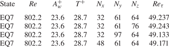
Domain sizes and grid numbers of the flow configuration used in the present study. Four pairs of equilibria are considered in total, i.e. one in  $\varOmega _{N}$ and four (including an edge state, PO) in
 $\varOmega _{HKW}$.

In the present study, the Reynolds number is chosen to be  $Re=400$, which gives
 ${Re_{\tau }}=33.3$ and
 $33.9$ for the two computational domains
 $\varOmega _N$ and
 $\varOmega _{HKW}$, respectively (see also table 2). This choice is made to study the dynamics of near-wall coherent structure primarily, such that the computational domain becomes the well-known minimal flow unit (Jiménez & Moin Reference Jiménez and Moin1991; Hamilton et al. Reference Hamilton, Kim and Waleffe1995): for example, the inner-scaled domain size of
 $\varOmega _{HKW}$ is
 $(L_x^{+},L_y^{+},L_z^{+})=(186,67.8,133)$, just large enough to study the dynamics of a single pair of low/high-speed streaks and the related quasi-streamwise vortices. With this choice, the dynamical systems approach involving the computation of equilibrium solutions and unstable periodic orbits becomes a useful tool to study the turbulence dynamics. In this respect, it should be mentioned that the understanding to be gained from this study would be limited precisely to the near-wall coherent structure dynamics, which has been understood to be largely independent of the outer flow (Jiménez & Pinelli Reference Jiménez and Pinelli1999; Hwang Reference Hwang2013).
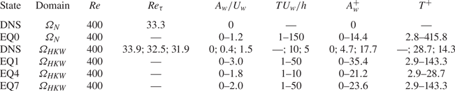
Control parameters for the studied cases. The superscript  $+$ indicates normalisation by viscous inner units of the corresponding uncontrolled DNS of each computational domain. Cases A and B studied in § 3 are EQ0 with
 $Re=400$,
 ${T^{+}}=166.4$,
 ${A_w^{+}}=2.6$ and
 $4.4$, respectively. The semicolons referring to the DNS in
 $\varOmega _{HKW}$ separate the uncontrolled and controlled cases.

2.1. Spanwise wall oscillation control
The spanwise wall oscillation applies the following control law to the walls:
 \begin{equation} W_w(t) = {A_w} \sin(2{\rm \pi} t/T), \end{equation}
where  $W_w(t)$ is the spanwise velocity at the walls,
 ${A_w}$ is the amplitude of the spanwise wall velocity,
 $T$ is the wall oscillation period, and
 $t$ is the time. In this study, the upper and lower walls are set to oscillate in phase in the spanwise direction, i.e.
 $W_w(t)|_{y=0} = W_w(t)|_{y=2h}$. The control is applied to a set of equilibrium solutions and DNS by varying
 ${A_w}$ and
 $T$, as summarised in table 2. The parameters are also scaled by viscous inner units of the uncontrolled DNS in the corresponding computational domain, so that
 $A^{+}_w={A_w}/{u_{\tau }}$ and
 ${T^{+}}=T{u_{\tau }}^{2}/\nu$, where
 ${u_{\tau }}=\sqrt {\tau _w/\rho }$ is the skin-friction velocity with
 $\tau _w= \mu \langle \overline {\partial u/ \partial y}|_{y=0,2h }\rangle _{x,z}$ being the streamwise wall shear stress of the uncontrolled DNS at
 $Re=400$ unless stated otherwise. Here,
 $\langle \cdot \rangle _{x,z}$ indicates the average in streamwise and spanwise directions, and
 $\overline {(\cdot )}$ indicates the time average. The skin-friction coefficient is defined as
 ${C_f}=2\tau _w/(\rho {U_w}^{2})=2({Re_{\tau }}/Re)^{2}$, where
 ${Re_{\tau }}={u_{\tau }}h/\nu$ is the friction Reynolds number. The spanwise wall oscillation control has been implemented and verified in our previous study for plane Poiseuille flow (Yang & Hwang Reference Yang and Hwang2019) by comparing with the DNS data of Hurst et al. (Reference Hurst, Yang and Chung2014). Following previous studies (e.g. Hurst et al. Reference Hurst, Yang and Chung2014), we define the drag reduction rate
 $\mathcal {DR}$ as the relative change in the
 ${C_f}$ values between the controlled and uncontrolled states, i.e.
 \begin{equation} \mathcal{DR}\,(\%) = \frac{C_{f,0} - {C_f}}{C_{f,0}}, \end{equation}
where  $C_{f,0}$ is the skin-friction coefficient of the uncontrolled state.
2.2. Computation of equilibrium solutions and edge states
In this study, we consider four pairs of equilibrium states (lower- and upper-branch solutions): EQ0 in  $\varOmega _{N}$ (Nagata Reference Nagata1990) and EQ1, EQ4, EQ7 in
 $\varOmega _{HKW}$ (Gibson et al. Reference Gibson, Halcrow and Cvitanovic2008), which are listed in table 1. As discussed in § 1, the lower branch of the solutions has low drag and has been associated with the dynamics of the ‘edge’, the laminar-turbulent state space separatrix, while the upper branch is characterised with high drag and exhibits many features of turbulent state – note that the term ‘branch’ implies each member of a solution pair. The equilibrium states are computed using the Newton–Krylov–Hookstep method (Viswanath Reference Viswanath2007; Willis et al. Reference Willis, Cvitanović and Avila2013). The algorithm finds the equilibrium states by zeroing numerically the relative error between the initial condition and the following final solution translated in time and space at
 $t=T_0$:
 \begin{equation} r= \frac{\| \sigma ({-}s_x,-s_z )\,\varPhi^{T_0} (\boldsymbol{u}) - \boldsymbol{u} \|}{\| \boldsymbol{u} \|}, \end{equation}
where  $\boldsymbol {u}$ is the initial state,
 $\varPhi ^{T_0} (\boldsymbol {u})$ is the state at
 $t=T_0$ with the state transition operator
 $\varPhi ^{t}(\cdot )$, and
 $r$ is the relative error. Here
 $\sigma (-s_x,-s_z)$ is the spatial shift operator representing a translation by distance
 $s_x$ in the streamwise direction and
 $s_z$ in the spanwise direction, i.e.
 $\sigma (-s_x,-s_z)\,\boldsymbol {u}(x,y,z)=\boldsymbol {u}(x-s_x,y,z-s_z)$. In the present study, the relative error
 $r<10^{-8}$ is chosen for all the solutions, which gives good numerical convergence. The equilibrium solutions from Gibson et al. (Reference Gibson, Halcrow and Cvitanovic2008) (http://channelflow.org/dokuwiki/doku.php?id=database) were taken as the starting point for our Newton iteration. The period
 $T_0$ can be fixed arbitrarily for uncontrolled cases as the equilibrium states in this study are time-independent, and
 $T_0=8h/{U_w}$ is chosen. However, under the spanwise wall oscillation, the flow shows a periodicity due to the presence of periodic wall motion, thus the time interval needs to satisfy
 $T_0=n T$, where
 $T$ is the spanwise wall oscillation period, and
 $n$ is a positive integer number. In general, there is no reason for
 $T_0$ and
 $T$ to be identical (i.e.
 $n=1$), as they are different quantities – we have also tested the solution procedure with different
 $n$ values (
 $n=2,3$, in particular) for a few solutions, and the converged solutions were found to not depend on
 $n$ at least in those cases (see also figure 6). However, if
 $n > 1$ is chosen, then it may be possible for the given solution procedure to capture incidentally unwanted exact solutions with nonlinearly saturated subharmonic/modulational instabilities. In such a case, the computed solutions would not be a homotopy of the original solution, as their primary time periodicity is no longer
 $T$. Furthermore, for a very large
 $n$, the Newton iteration does not converge quickly with a very small
 $r$ due to the unstable nature of the solutions, and the related computation also becomes very expensive due to many simulations required over a long time interval. For this reason,
 $n=1$ is chosen in the present study. In the absence of the spanwise wall oscillation, all the considered equilibria (EQ0, EQ1, EQ4 and EQ7) in this study satisfy the shift–reflect symmetry
 \begin{equation} [u,v,w,p](x,y,z)= [u,v,-w,p](x-{L_x}/2,y,-z), \end{equation}
where  $p$ is the pressure. However, under this symmetry, the streamwise uniform spanwise wall velocity vanishes, and the spanwise wall oscillation cannot be implemented. Therefore, the condition (2.4) is relaxed for the computation of ECS in the presence of spanwise wall oscillation. The solutions are then computed using a pseudo arc-length continuation algorithm in the parameter space,
 $(Re, {A_w}, T)$. The linear stability of each equilibrium solution is also performed by solving the corresponding eigenvalue problem via the Arnoldi iteration.
The edge state is also calculated using the standard bisection technique (Itano & Toh Reference Itano and Toh2001; Skufca et al. Reference Skufca, Yorke and Eckhardt2006). This approach builds an initial guess by weighting two states, one of which is towards a turbulent state and the other towards a laminar state. For this calculation, we introduce the turbulent fluctuation energy averaged over a given computational domain,
 \begin{equation} (E_{uu},E_{vv},E_{ww})=\frac{1}{2V} \int_\varOmega (u^{\prime 2}, v^{\prime 2}, w^{\prime 2}) / {U_w}^{2} \,{{\rm d}}V, \end{equation}
where  $u^{\prime }$,
 $v^{\prime }$ and
 $w^{\prime }$ are defined from the Reynolds decomposition
 $\boldsymbol {u}=\boldsymbol {U}+\boldsymbol {u}^{\prime }$, with
 $\boldsymbol {U}=(U,V,W)$ being the streamwise, wall-normal and spanwise velocities averaged over time and in the wall-parallel directions, and
 $\boldsymbol {u}'=(u',v',w')$ the remaining velocity fluctuations. The bisection method is carried out by monitoring the cross-streamwise velocity fluctuation energy (
 $E_{vv} + E_{ww}$). The edge state investigated in this study is a periodic orbit obtained in the domain
 $\varOmega _{HKW}$, which is identical to the gentle periodic solution found by Kawahara & Kida (Reference Kawahara and Kida2001) and is denoted as PO in table 1. This periodic orbit is used as the initial guess in the Newton–Krylov–Hookstep solver with its specific period to complete its bifurcation diagram.
2.3. Physical relevance to exact coherent states in fully developed turbulence
Before presenting the result of the present study, some physical relevance of the ECS is discussed here. ECS refer to equilibrium solutions and unstable periodic orbits of the Navier–Stokes equations that resemble coherent structures and their dynamics. Typically, these solutions are unstable, and the turbulence trajectory visits them only transiently, making them difficult to be observed directly for a long time in typical laboratory experiments and numerical simulations (e.g. Hof et al. Reference Hof, van Doorne, Westerweel, Nieuwstadt, Faisst, Eckhardt, Wedin, Kerswell and Waleffe2004; Kerswell & Tutty Reference Kerswell and Tutty2007). However, once many solutions are available, turbulence may be described as a random walk around these solutions. From this viewpoint, these solutions have been believed to form the state space skeleton of turbulence (Kerswell Reference Kerswell2005; Eckhardt et al. Reference Eckhardt, Schneider, Hof and Westerweel2007; Kawahara et al. Reference Kawahara, Uhlmann and van Veen2012; Graham & Floryan Reference Graham and Floryan2021), playing a role of guiding the solution trajectory in the state space, and indeed this has been confirmed, at least in the minimal flow units considered in the present study (e.g. Gibson et al. Reference Gibson, Halcrow and Cvitanovic2009; Willis et al. Reference Willis, Cvitanović and Avila2013). Exact coherent states have also been computed for external flows where aerodynamic applications would be relevant (Khapko et al. Reference Khapko, Kreilos, Schlatter, Duguet, Eckhardt and Henningson2013; Kreilos et al. Reference Kreilos, Gibson and Schneider2016a, ). Extending this approach to high Reynolds numbers is an important ongoing open research topic, although some previous efforts were made by modelling small scales using eddy viscosity (e.g. Hwang et al. Reference Hwang, Willis and Cossu2016; Yang & Hwang Reference Yang and Hwang2019).
3. Results and discussion
3.1. Bifurcation diagram of EQ states
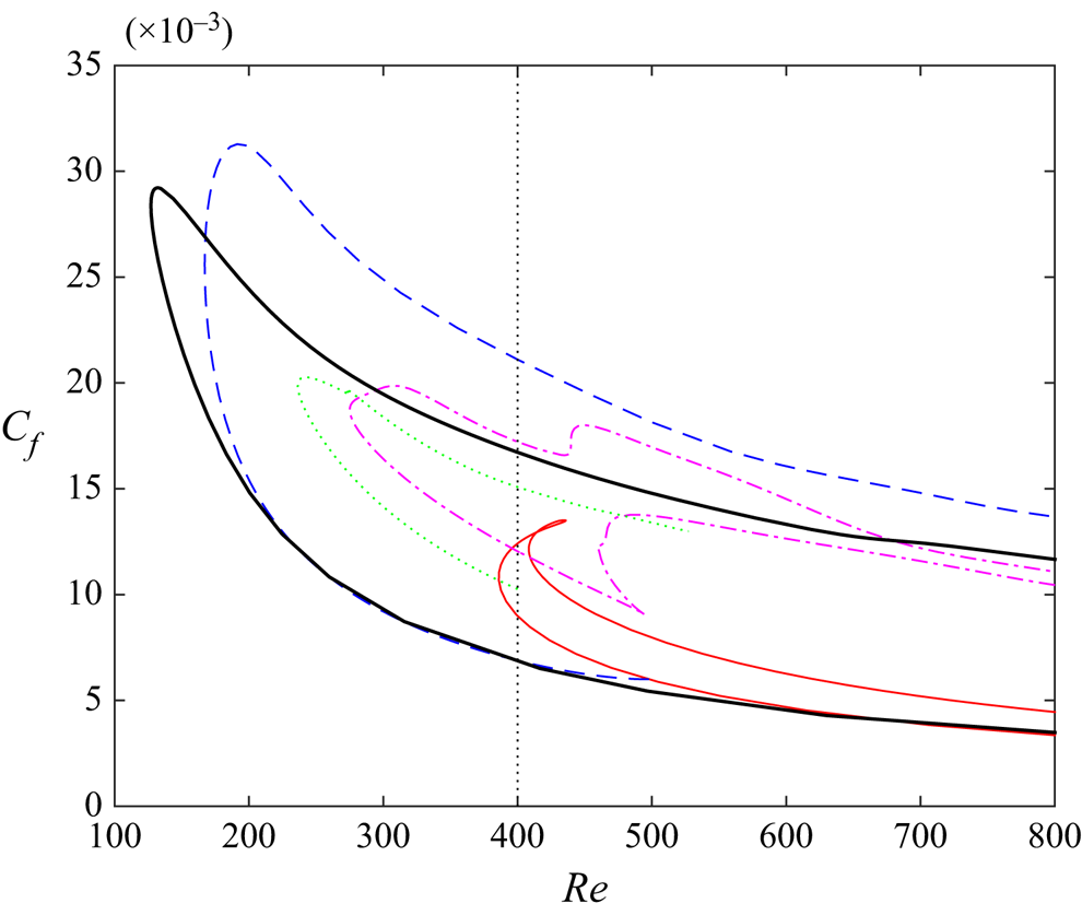
The bifurcation diagram of the various equilibrium solutions is shown in figure 1. Each of the solutions emerges through a saddle–node bifurcation. The solution that appears at the smallest Reynolds number is EQ0 from Nagata (Reference Nagata1990) at critical Reynolds number  ${Re_c} \approx 127$, followed by EQ7 at
 ${Re_c} \approx 167$ from Gibson et al. (Reference Gibson, Halcrow and Cvitanovic2009). The numerical continuation over the computational domain size indicates that EQ7 does not exist in the domain
 $\varOmega _N$, and EQ0 does not exist in the domain
 $\varOmega _{HKW}$. A large number of solutions, including EQ1, EQ4 and EQ7, were found previously in
 $\varOmega _{HKW}$. The bifurcation curves for EQ1 and EQ4 are more complicated. EQ1 appears through a saddle–node bifurcation at
 ${Re_c}=386$, then second and third bifurcations occur on the upper branch at
 ${Re_c}=408$ and
 $435$, respectively. EQ4 first arises from a saddle–node bifurcation at
 ${Re_c}=275$, then a second saddle–node bifurcation appears at
 ${Re_c}=494$ from the lower branch, and at
 ${Re_c}=438$ from the upper branch, respectively, giving rise to a new branch. For further details about the invariant solutions in
 $\varOmega _{HKW}$, the reader may refer to Gibson et al. (Reference Gibson, Halcrow and Cvitanovic2009). The bifurcation curve for a periodic orbit (PO) identified in
 $\varOmega _{HKW}$ is also presented in the figure by a green dotted line. The saddle–node bifurcation behaviour of PO is very similar to that of EQ0 and EQ7, with a critical Reynolds number located at
 ${Re_c}=236.5$.
Bifurcation diagram of the equilibrium solutions in the  ${C_f}$–
 $Re$ plane: EQ0, black thick solid line; EQ1, red thin solid line; EQ4, pink dash-dotted line; EQ7, blue dashed line; PO, green dotted line. The vertical dashed line indicates
 $Re=400$.

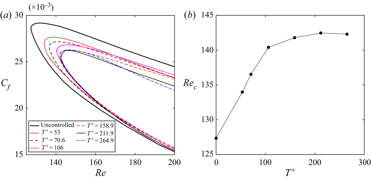
It is known that there is an optimal oscillation period at  ${T^{+}} \approx 100$ for spanwise wall oscillation control. Focusing on EQ0, we show that such an optimal oscillation period appears in the bifurcation diagram. Figure 2(a) presents the bifurcation curves for EQ0 with six different oscillation periods in the range
 $T {U_w}/h\in [1,150]$ for a given wall oscillation amplitude
 ${A_w}/{U_w}=0.1$. As the focus is on the saddle–node point, here the viscous wall units of the uncontrolled saddle–node point are used for the scaling of the oscillation period, which is more meaningful to identify the inner scaled optimal wall oscillation period. This gives
 ${T^{+}}=53$,
 $70.6$,
 $106$,
 $158.9$,
 $211.9$ and
 $264.9$ for the six studied cases. Here, the amplitude
 ${A_w}$ is selected deliberately to be small such that the solutions can exist at large oscillation periods, as will be discussed at the end of this section. As can be seen, the lower branch is much less affected by the control compared to the upper branch. The saddle–node point continues to move towards higher values as the oscillation period
 ${T^{+}}$ is increased, from
 ${Re_c}=127.3$ of the uncontrolled case to
 ${Re_c}=140.4$ at
 ${T^{+}}=106$ and
 ${Re_c}=142.5$ at
 ${T^{+}}=211.9$, then moves back to
 ${Re_c}=142.2$ at
 ${T^{+}}=264.9$. This indicates that the emergence of the unstable solutions is delayed to higher Reynolds numbers, implying the suppression of these solutions, a primitive form of turbulence. We note that the decreasing rate of
 ${Re_c}$ becomes slower eventually as
 ${T^{+}}$ becomes larger, and
 ${Re_c}$ increases only slightly for
 ${T^{+}}>106$. The skin friction of the upper branch does not decrease after
 ${T^{+}}>70.6$ at
 $Re\approx 170$. For larger oscillation periods, it was difficult to obtain converged solutions, and we were not able to continue numerically for
 ${T^{+}}>264.9$ with EQ0. The critical Reynolds number variation at the saddle–node point with the wall oscillation period is presented in figure 2(b). It is clear that the saddle–node Reynolds number saturates for
 ${T^{+}}>106$, consistent with the optimal oscillation period (i.e.
 ${T^{+}}\approx 100$) as observed in the DNS data as well as our previous bifurcation study of the wall-attached ECS under spanwise wall oscillation in Poiseuille flow (Yang & Hwang Reference Yang and Hwang2019), although the present solution shows a broader optimal
 ${T^{+}}$ regime for drag reduction compared to that of fully developed turbulence at much higher Reynolds numbers.
(a) Plots of  ${C_f}$–
 $Re$ bifurcation curves for EQ0 with different oscillation periods at
 ${A_w}/{U_w}=0.1$. (b) The saddle–node Reynolds number variation with the oscillation period. Here, the wall units of the uncontrolled case at the saddle–node point are used for the scaling of the wall oscillation periods.

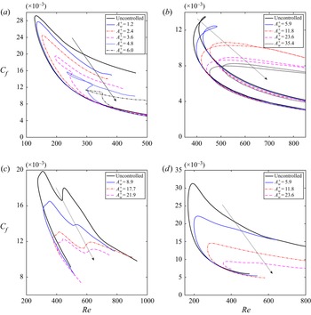
In figure 3, we show the bifurcation curves of the equilibrium solutions EQ0, EQ1, EQ4 and EQ7 in the  ${C_f}$–
 $Re$ plane for different spanwise wall oscillation amplitudes, each of which has a lower and an upper branch subject to the spanwise wall oscillation. The thick solid lines represent the uncontrolled reference cases of each equilibrium solution. For each solution, we fix the wall oscillation period
 ${T^{+}}$ and choose different values of amplitude
 ${A_w^{+}}$. As mentioned in table 2, here the viscous inner units of the corresponding uncontrolled DNS of each computational domain at
 $Re=400$ are used for the scaling. The upper branch of each equilibrium solution pair shows a significant skin-friction reduction as
 ${A_w^{+}}$ is increased. This strong effect on the upper branch of each solution leads to the emergence of sophisticated bifurcations along the upper branch on increasing
 ${A_w^{+}}$ (figures 3(a,b), in particular), although there is no common trend in those bifurcations. It is noted that the monotonic decrease of the
 ${C_f}$ value of the upper branch solution with the increase of
 ${A_w^{+}}$ is analogous to the effect of
 ${A_w^{+}}$ on turbulent drag reduction in fully developed turbulence at much higher Reynolds numbers (Quadrio & Ricco Reference Quadrio and Ricco2004; Quadrio et al. Reference Quadrio, Ricco and Viotti2009). On the contrary, the effect on the lower branch is nearly negligible over almost the entire range of Reynolds numbers. The effect of control on the lower branch is, however, not monotonic. We observe a slight decrease of
 ${C_f}$ for sufficiently high Reynolds numbers, while the skin-friction coefficient near the saddle–node point increases until the lower and upper branches collapse and disappear. As a consequence, the saddle–node bifurcation points move towards higher Reynolds numbers, indicating stabilisation of the equilibrium solutions.
Bifurcation curves at different values of wall oscillation amplitudes  ${A_w^{+}}$ in the
 ${C_f}$–
 $Re$ plane: (a) EQ0 with
 ${T^{+}}=79.8$; (b) EQ1 with
 ${T^{+}}=14.3$; (c) EQ4 with
 ${T^{+}}=14.3$; (d) EQ7 with
 ${T^{+}}=28.7$. Thick solid curves correspond to the uncontrolled reference cases. The arrows indicate increasing
 ${A_w^{+}}$.

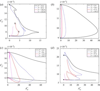
Figure 4 shows further the bifurcation curves of the skin-friction coefficient with respect to the wall oscillation amplitude  ${A_w^{+}}$ for various oscillation periods
 ${T^{+}}$ at
 $Re=400$. In general, commonly the upper branches of the solutions exhibit a significant reduction in
 $C_f$ on increasing
 ${A_w^{+}}$, consistent with figure 3. On the contrary,
 $C_f$ values of the lower branches depend on the individual solutions and the time period considered (see figure 4). However, the significant reduction of
 $C_f$ in the upper branch leads the two branches to meet at a certain value of
 ${A_w^{+}}$, forming a saddle–node bifurcation in terms of
 ${A_w^{+}}$. An increase of the wall oscillation period
 ${T^{+}}$ yields the solutions to form the saddle–node point at lower values of
 ${A_w^{+}}$. However, it should be mentioned that this behaviour may well be true only for the values of
 ${T^{+}}$ considered here, as the numerical continuation of the solutions (upper branches, in particular) is found to be difficult for very large
 ${T^{+}}$.
Bifurcation curves  ${C_f}$–
 ${A_w^{+}}$ for different oscillation periods
 ${T^{+}}$ at
 $Re=400$: (a) EQ0, (b) EQ1, (c) EQ4, (d) EQ7. The black filled circles and squares indicate the lower and upper branch solutions, respectively, at
 ${A_w^{+}}=0$. The open circle and triangle in (a) indicate, respectively, case A (
 $Re=400$,
 ${T^{+}}=166.4$,
 ${A_w^{+}}=2.6$) and case B (
 $Re=400$,
 ${T^{+}}=166.4$,
 ${A_w^{+}}=4.4$) presented in table 2.

3.2. Statistics
The spanwise wall oscillation generates an unsteady near-wall spanwise shear layer referred to as the Stokes layer (according to the Stokes’ second problem). For the laminar case, the flow introduced by the spanwise wall motion is decoupled from the streamwise flow, and the unsteady Stokes layer can be expressed analytically as (Schlichting Reference Schlichting1979)
 \begin{equation} W(y,t) = {A_w} \,{\rm e}^{-\eta}\sin(2{\rm \pi} t/T - \eta), \end{equation}
where  $\eta = -y\sqrt {{\rm \pi} \,Re/T}$ is related to the Stokes layer thickness. A larger spanwise wall oscillation period leads to a thicker Stokes layer, and for a given oscillation period, the wall oscillation amplitude only affects the spanwise displacement of the wall. Because of the presence of two walls, (3.1) is, however, not valid in this context, especially when the Stokes layer thickness is comparable to the half channel width. Therefore, we have considered further the analytical solution for the uniform spanwise wall oscillation problem in channel flow, derived by Jozsa (Reference Jozsa2019). This solution is given by
 \begin{equation} W(y,t) = {{\rm Re}}{\left({A_w} \exp({{\rm i}2{\rm \pi} t/T})\, \frac{\cos(y\sqrt{-{\rm i}2{\rm \pi}\,Re/T})} {\cos(\sqrt{-{\rm i}2{\rm \pi}\,Re/T})}\right)}, \end{equation}
where  ${{\rm Re}}(\cdot )$ indicates the real part.
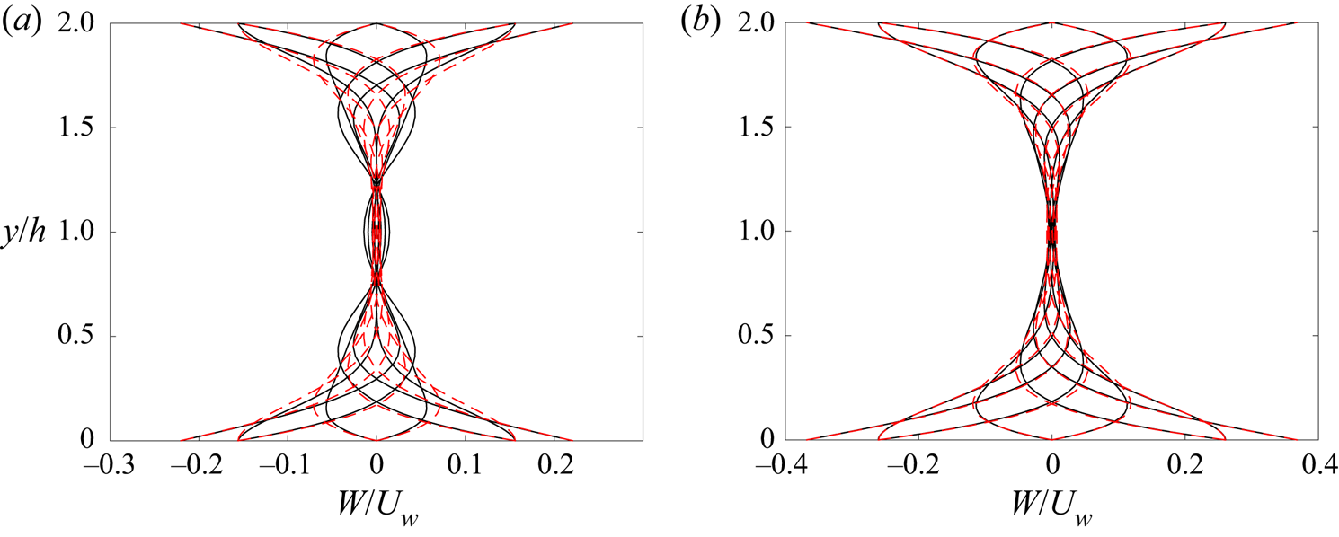
In figure 5, we present the Stokes layer at eight equally separated phases for cases A and B of the EQ0 state (see also figure 4a). With the given wall oscillation period  ${T^{+}}=166.4$, the analytical profiles of the Stokes layer decay to zero only near the channel centre. As the spanwise Stokes layer is affected by the equilibrium state, the Stokes layer profiles of EQ0 under control start to deviate from the analytical ones. We note that such a deviation is small in the region close to the wall, but becomes large away from the wall (see figure 5a). In general, it is found that at a small oscillation period, the Stokes layer is thin and the agreement with the analytical solution is improved (not shown here). This is because the Stokes layer of the equilibrium state is obtained from the spanwise mean momentum balance and is determined by the contribution from the wall-normal gradient of the spanwise Reynolds shear stress term
 $\partial \overline {v'w'} / \partial y$, which has been found to increase with the oscillation period and the Reynolds number (Ricco & Quadrio Reference Ricco and Quadrio2008; Yang Reference Yang2016). At a higher drag state, such as case A shown in figure 5(a), the Stokes layer of the equilibrium state differs largely from that of the analytical solution in (3.2), and some oscillating flow even appears in the channel centre. On the contrary, the agreement of the Stokes layer between the equilibrium state and the analytical solution is greatly improved for a lower drag state of case B (figure 5b). It is noted that under the control parameters for cases A and B, the difference between the analytical solutions from (3.1) and (3.2) is small.
Unsteady spanwise Stokes layer at  $8$ equally separated phases for: (a) case A (
 $Re=400$,
 ${T^{+}}=166.4$,
 ${A_w^{+}}=2.6$), and (b) case B (
 $Re=400$,
 ${T^{+}}=166.4$,
 ${A_w^{+}}=4.4$). The solid and dashed lines indicate, respectively, the equilibrium state of EQ0 and the analytical solution in (3.2).

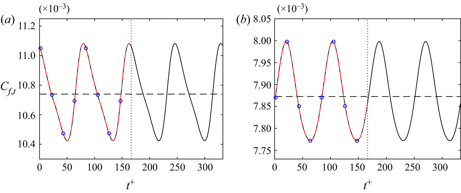
The time variations of the instantaneous skin-friction coefficient  $C_{f,t}$ for cases A and B are shown in figure 6. For the spanwise wall oscillation cases, the statistics is sampled and averaged over one single wall oscillation period for the converged solution, i.e.
 ${C_f}=({1}/{T})\int _0^{T} C_{f,t}\,\mathrm {d}t$. Each solution is computed and compared with two different values of
 $n$ (i.e.
 $n=1, 2$) used for the calculation (see § 2.2). As expected, the converged solution does not depend on
 $n$, except that the solution with
 $n=2$ simply repeats that of
 $n=1$ twice. As already mentioned for figure 4(a), case A is a higher drag state with
 ${C_f}=0.0107$, while case B is a lower drag state with
 ${C_f}=0.0079$. Based on the derivation of the wave pattern of
 $C_{f,t}$ in time compared to the sinusoidal wall oscillation wave, the equilibrium solution of case A is modulated more strongly by the spanwise wall oscillation compared to that of case B, and each solution has the
 $C_{f,t}$ variation of
 $3.2\,\%$ and
 $1.6\,\%$ during one wall oscillation period, respectively. It is noted that the skin-friction coefficient for the upper branch of the uncontrolled EQ0 state at
 $Re=400$ is
 ${C_f}=0.0167$, thus the two controlled cases have drag reduction
 $\mathcal {DR}=35.9\,\%$ and
 $52.7\,\%$, respectively.
Variation of instantaneous skin-friction coefficient  $C_{f,t}$ over time for (a) case A (
 $Re=400$,
 ${T^{+}}=166.4$,
 ${A_w^{+}}=2.6$), and (b) case B (
 $Re=400$,
 ${T^{+}}=166.4$,
 ${A_w^{+}}=4.4$). The red dashed (black solid) lines are for equilibrium solutions computed with
 $n=1$ (
 $n=2$) in the Newton solver. The horizontal lines indicate the mean value of the skin-friction coefficient, i.e.
 ${C_f}=0.0107$ and
 $0.0079$ for cases A and B, respectively. The vertical dotted lines mark one wall oscillation period,
 ${T^{+}}=166.4$. The blue circles mark the
 $8$ equally separated phases investigated for each case, i.e.
 $\phi =0$,
 ${\rm \pi} /4$,
 ${\rm \pi} /2$,
 $3{\rm \pi} /4$,
 ${\rm \pi}$,
 $5{\rm \pi} /4$,
 $3{\rm \pi} /2$,
 $7{\rm \pi} /4$.

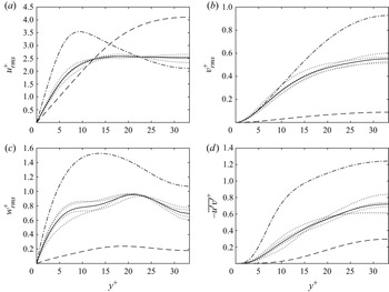
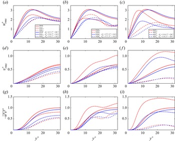
Figure 7 shows the root-mean-square (r.m.s.) velocity components, i.e.  ${u_{rms}^{+}}$,
 ${v_{rms}^{+}}$,
 ${w_{rms}^{+}}$, and the streamwise Reynolds shear stress
 $-\overline {u'v'}^{+}$ profiles for case A at
 $8$ equally separated phases (dotted lines) over one wall oscillation period (see symbols in figure 6a). The phase variation in the statistics becomes clear with a modest value, which corresponds to
 $3.2\,\%$ variation in the skin friction (figure 6a). It is interesting to note that the r.m.s. profiles of the controlled state A appear to sit between those of the upper- and lower-branch solutions. For example, the upper-branch solution shows a strong near-wall peak in
 ${u_{rms}^{+}}$, while such a peak is located in the channel centre for the lower-branch solution. The controlled state A exhibits the two features in a mixed manner – the strength of
 ${u_{rms}^{+}}$ in the channel centre is increased compared to the upper branch, while the
 ${u_{rms}^{+}}$ peak in the near-wall region is weakened (figure 7a). The rest of the profiles behave in a similar manner (figures 7b–d). Furthermore, the reduction of
 $-\overline {u'v'}^{+}$ over the entire wall-normal locations compared to the upper-branch solution indicates a drag reduction according to the FIK identity (Fukagata, Iwamoto & Kasagi Reference Fukagata, Iwamoto and Kasagi2002) – indeed,
 $35.9\,\%$ of
 $\mathcal {DR}$ from the upper-branch solution is observed. Similar statistics features are also observed from the other exact coherent states in the domain
 $\varOmega _{HKW}$, which are presented in Appendix B.
Root-mean-square (r.m.s.) velocity profiles scaled with viscous inner units of the uncontrolled DNS for case A ( $Re=400$,
 ${T^{+}}=166.4$,
 ${A_w^{+}}=2.6$): (a)
 $u_{rms}^{+}$, (b)
 $v_{rms}^{+}$, (c)
 $w_{rms}^{+}$, and (d)
 $-\overline {u^{\prime }v^{\prime }}^{+}$. Dash-dotted (dashed) lines represent the upper (lower) branch of the uncontrolled state, and dotted lines indicate the controlled state at
 $8$ equally separated phases, with the mean profile indicated by the solid line.

3.3. Streak variation
Now, the time and space variations of the streaks are studied using cases A and B of EQ0. We note that the choice of EQ0 is made because it appears to be more useful than the other solutions for the following reasons. First, currently EQ0 is known as the invariant solution emerging at the lowest Reynolds number in plane Couette flow. Importantly, turbulence emerges directly from the upper branch of EQ0 through a bifurcation cascade (Kreilos & Eckhardt Reference Kreilos and Eckhardt2012) – note that all the other equilibrium solutions considered here do not have this feature. Furthermore, the skin friction of the upper branch of EQ0, often believed to be more relevant to the turbulent state, is  $C_f=0.0168$ at
 $Re=400$, not very far from the time-averaged turbulent state with
 $C_f=0.0138$ at the same Reynolds number. Finally, at
 $Re=400$, the lower branch of EQ0 is the edge state in the domain
 $\varOmega _N$ (Schneider et al. Reference Schneider, Gibson, Lagha, De Lillo and Eckhardt2008). A particular feature for spanwise wall oscillation control of turbulence is the modulation of the near-wall streaks by the Stokes layer, which has been studied extensively using instantaneous flow fields or conditionally averaged flow structures obtained from DNS. As a result, some key dynamical features of the controlled flow may not be well observed in the complex three-dimensional flow field or are averaged out in the conditional flow fields. Such a drawback may be bypassed by inspecting some equilibrium solutions modulated by the Stokes layer, as they are the exact solutions of the Navier–Stokes equations.
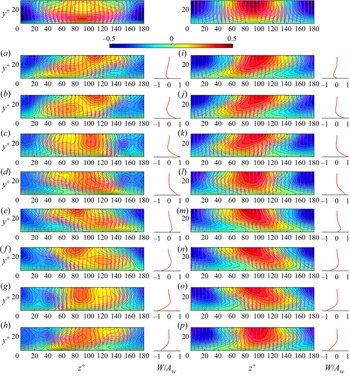
Figure 8 presents the streamwise-averaged streaks visualised by  $\langle u' \rangle _x$ contour and the vortical motions visualised by
 $( \langle v' \rangle _x, \langle w' \rangle _x - \langle w' \rangle _{x,z} )$ vectors for cases A and B. The features of the upper- and lower-branch solutions of EQ0 at
 $Re=400$ without control are shown in the top row of figure 8. It is clear that the shapes of the low- and high-speed streaks of the lower-branch solution are almost symmetrical to each other, while this is not the case for the upper-branch solution, with the high-speed streak spreading a much wider area in the spanwise direction of the near-wall region and the low-speed streak more localised. Therefore, in the upper-branch solution, the high-speed streak is expected to make a strong contribution to the elevation of local skin friction, and this should be significantly greater than the local reduction created by the low-speed streak.
Streamwise-averaged low- and high-speed streaks (contour by  $\langle u' \rangle _x$) and in-plan vortex (arrows plotted by (
 $\langle v' \rangle _x, \langle w' \rangle _x - \langle w' \rangle _{x,z}$)) variation during one oscillation period for (a–h) case A (
 $Re=400$,
 ${T^{+}}=166.4$,
 ${A_w^{+}}=2.6$), and (i–p) case B (
 $Re=400$,
 ${T^{+}}=166.4$,
 ${A_w^{+}}=4.4$), at different phases: (a,i)
 $\phi =0$; (b,j)
 $\phi ={\rm \pi} /4$; (c,k)
 $\phi ={\rm \pi} /2$; (d,l)
 $\phi =3{\rm \pi} /4$; (e,m)
 $\phi ={\rm \pi}$; ( f,n)
 $\phi =5{\rm \pi} /4$; (g,o)
 $\phi =3{\rm \pi} /2$; (h,p)
 $\phi =7{\rm \pi} /4$. The Stokes profiles at the corresponding phases are shown on the right-hand side of each contour plot. The top row presents the flow fields of the corresponding upper- and lower-branch solutions of uncontrolled EQ0 at
 $Re=400$. Viscous inner units of the uncontrolled DNS case are used for the scaling.

Once spanwise wall oscillation is applied, the streaks are modulated significantly by the Stokes layer. For case A, (figures 8a–h), similarly to the upper-branch solution of the uncontrolled case, the high-speed streak is stronger than the low-speed one. However, under the control, the high-speed streak in the near-wall region is tilted strongly in the spanwise direction. In particular, the near-wall part of the high-speed streak penetrates deeply underneath the low-speed streak, and vice versa. Such a spanwise motion appears to enhance fluid mixing between the low- and high-speed streaks. Therefore, the locally high-friction region from the high-speed streaks is balanced out with the locally low-friction region from the low-speed streaks, resulting in a drag reduction – indeed, the asymmetry between the low- and high-speed streaks appears to be weaker than that of the upper-branch solution of the uncontrolled case (see figures 8d,h). For case B (figures 8i–p), a lower drag state, the low- and high-speed streaks are almost symmetric to each other, and their movements in the spanwise direction are nearly in phase. Moreover, the low- and high-speed streaks have the largest fluctuation in the channel centre. We also note that the streak variation in the spanwise direction is very similar to the conditionally averaged results in the DNS study by Touber & Leschziner (Reference Touber and Leschziner2012). This indicates that the equilibrium solutions in this study do capture some important dynamics of the near-wall flow under the spanwise wall oscillation, although the Reynolds number considered here is much lower than that of Touber & Leschziner (Reference Touber and Leschziner2012).
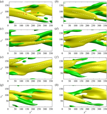
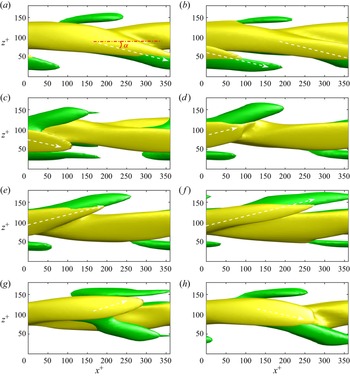
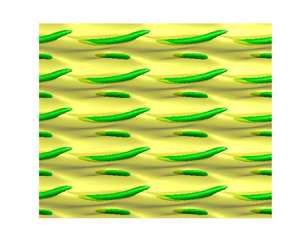
To explore further the streak angle variation during one wall oscillation period, the high-speed streak and vortical structure are visualised in figures 9 and 10 for cases A and B, respectively. At first glance, the structures for case A are more active than those for case B. During one oscillation period, two dominant streak-tilting angles are seen with opposite sign, as also observed in previous DNS studies (Touber & Leschziner Reference Touber and Leschziner2012; Chung et al. Reference Chung, Hurst and Yang2013). Each of these angles is seen dominantly for half an oscillation period. For cases A and B, these tilting angles of the streaks are found to be  $\alpha \approx \pm 18^{\circ }$ and
 $\alpha \approx \pm 14^{\circ }$, respectively. By monitoring the evolution of the streaks in figure 9, the high-speed streak is first tilted in the negative spanwise direction until
 $\phi = {\rm \pi}/2$, then breaks down suddenly into two streaks, a stronger one that grows fast, and a weaker one that dissipates quickly. By checking the temporal skin-friction variation of case A (see figure 6a), it is found that
 $C_{f,t}$ reaches its minimum value at the streak breakdown stage, while it reaches the peak value at the phase with the strongest streak. For case B (figure 6b), the switch from a negatively tilted streak to a positively tilted one (
 $\phi ={\rm \pi} /2\unicode{x2013}3{\rm \pi} /4$) is also very quick, but the streak breakdown process is not observed clearly as in case A.
Streak variation viewed from the bottom of the channel during one oscillation period for case A ( $Re=400$,
 ${T^{+}}=166.4$,
 ${A_w^{+}}=2.6$) at different phases: (a)
 $\phi =0$, (b)
 $\phi ={\rm \pi} /4$, (c)
 $\phi ={\rm \pi} /2$, (d)
 $\phi =3{\rm \pi} /4$, (e)
 $\phi ={\rm \pi}$, ( f)
 $\phi =5{\rm \pi} /4$, (g)
 $\phi =3{\rm \pi} /2$, and (h)
 $\phi =7{\rm \pi} /4$. A yellow isosurface (
 $u'^{+}=2.0$) indicates the high-speed streak, and a green isosurface (
 $v'^{+}=-0.2$) represents the vortical structure. The arrows represent the streak angle. Viscous inner units of the uncontrolled DNS are used for the scaling.

Streak variation viewed from the bottom of the channel during one oscillation period for case B ( $Re=400$,
 ${T^{+}}=166.4$,
 ${A_w^{+}}=4.4$) at different phases: (a)
 $\phi =0$, (b)
 $\phi ={\rm \pi} /4$, (c)
 $\phi ={\rm \pi} /2$, (d)
 $\phi =3{\rm \pi} /4$, (e)
 $\phi ={\rm \pi}$, ( f)
 $\phi =5{\rm \pi} /4$, (g)
 $\phi =3{\rm \pi} /2$, and (h)
 $\phi =7{\rm \pi} /4$. A yellow isosurface (
 $u'^{+}=2.0$) indicates the high-speed streak, and a green isosurface (
 $v'^{+}=-0.1$) represents the vortical structure. The arrows represent the streak angle. Viscous inner units of the uncontrolled DNS are used for the scaling.

Finally, it is worth mentioning that the tilting dynamics of the near-wall streaks is found to depend strongly on the strength of the Stokes layer. Unfortunately, this feature does not allow for a direct comparison with that observed in the previous DNS at high Reynolds numbers (Touber & Leschziner Reference Touber and Leschziner2012). In fact, as can be seen from figure 4, the equilibrium solutions of EQ1, EQ4 and EQ7 under the spanwise wall oscillation disappear at large wall oscillation amplitudes and periods. In other words, the Stokes layer, which was able to be examined here, was not strong enough to generate a large variation in the streak angle.
3.4. State space dynamics
Now, to visualise the relevant state space using state portraits, suitable observables are defined. Similarly to previous studies (e.g. Kawahara & Kida Reference Kawahara and Kida2001; Ibrahim et al. Reference Ibrahim, Yang, Doohan and Hwang2019), the volume-averaged equation for the mean kinetic energy (MKE) is first introduced:
 \begin{align} \frac{{{\rm d}}E_{\boldsymbol{U}}}{{{\rm d}}t} &= \underbrace{\frac{U_{w}\tau_{uw}}{h}}_{\mathcal{I}_U} - \underbrace{\frac{1}{V}\int_\varOmega -\langle { u^{\prime}v^{\prime}} \rangle_{x,z} \frac{\partial U}{\partial y}\,{{\rm d}}V}_{\mathcal{P}_{uv}} - \underbrace{\frac{\nu}{V} \int_{\varOmega} \left(\frac{\partial U}{\partial y}\right)^{2} {{\rm d}}V}_{\mathcal{D}_U} \nonumber\\ &\quad + \underbrace{\frac{W_w\tau_{ww}}{h}}_{\mathcal{I}_W} - \underbrace{\frac{1}{V}\int_{\varOmega} -\langle { v^{\prime}w^{\prime} }\rangle_{x,z}\, \frac{\partial W}{\partial y}\,{{\rm d}}V}_{\mathcal{P}_{vw}} - \underbrace{\frac{\nu}{V} \int_{\varOmega} \left(\frac{\partial W}{\partial y}\right)^{2} {{\rm d}}V}_{\mathcal{D}_W}, \end{align}
with the MKE given by
 \begin{equation} E_{\boldsymbol{U}}=\frac{1}{V}\int_\varOmega \boldsymbol{U}\boldsymbol{\cdot} \boldsymbol{U}\,{{\rm d}}V, \end{equation}
where  $\varOmega$ (
 $=\varOmega _N$ or
 $\varOmega _{HKW}$) is the given computational domain,
 ${U_w}$ and
 ${W_w}$ are the streamwise and spanwise velocities at the wall, and
 $\tau _{uw}=\mu \langle \partial u/\partial y|_{y=0,2h} \rangle _{x,z}$ and
 $\tau _{ww}=\mu \langle \partial w/ \partial y|_{y=0,2h} \rangle _{x,z}$ are the spatial averaged streamwise and spanwise wall shear stresses, respectively. The terms indicated by
 $\mathcal {I}_U$,
 $\mathcal {P}_{uv}$ and
 $\mathcal {D}_U$ in the first line of (3.3a) are the rate of energy input, the rate of energy transport by streamwise mean shear to turbulent kinetic energy (TKE), and the dissipation rate by the streamwise mean velocity, respectively. Similarly, the three terms in the second line, i.e.
 $\mathcal {I}_W$,
 $\mathcal {P}_{vw}$ and
 $\mathcal {D}_W$, correspond to the rate of energy input by the spanwise wall oscillation, the rate of energy transport by the spanwise mean shear to TKE, and the dissipation rate by the spanwise mean velocity.
The volume-averaged equation for TKE is also written as
 \begin{equation} \frac{{{\rm d}}E_{\boldsymbol{u}}}{{{\rm d}}t}= \underbrace{\frac{1}{V}\int_\varOmega -{\langle u^{\prime}v^{\prime}\rangle}_{x,z}\, \frac{\partial U}{\partial y}\,{{\rm d}}V}_{\mathcal{P}_{uv}} + \underbrace{\frac{1}{V} \int_\varOmega -{\langle v^{\prime}w^{\prime} \rangle}_{x,z}\, \frac{\partial W}{\partial y}\,{{\rm d}}V}_{\mathcal{P}_{vw}} - \underbrace{\frac{\nu}{V} \int_\varOmega \langle (\boldsymbol{\nabla} \boldsymbol{u^{\prime}})^{2} \rangle_{x,z}\,{{\rm d}}V}_{\mathcal{D}_{\boldsymbol{u}}}, \end{equation}
with  $E_{\boldsymbol {u}}=E_{uu}+E_{vv}+E_{ww}$ from (2.5). Here, the first two terms,
 $\mathcal {P}_{uv}$ and
 $\mathcal {P}_{vw}$, are identical to those of (3.3a), but with opposite signs, emerging as the rate of turbulence production by streamwise and spanwise mean shear, and the last term,
 ${\mathcal {D}_{\boldsymbol {u}}}$, is the TKE dissipation. For details about the derivation of (3.3a) and (3.4), the reader may refer to Ricco et al. (Reference Ricco, Ottonelli, Hasegawa and Quadrio2012). Finally, the rate of total energy input and dissipation are given by
 $\mathcal {I}\equiv \mathcal {I}_U+\mathcal {I}_W$ and
 $\mathcal {D}\equiv \mathcal {D}_U+\mathcal {D}_W+{\mathcal {D}_{\boldsymbol {u}}}$, respectively.
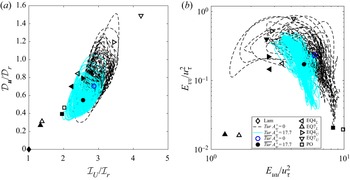
Two state portraits from the domain  $\varOmega _{HKW}$ at
 $Re=400$ are plotted in the
 $\mathcal {I}_U$–
 $\mathcal {D}_{\boldsymbol {u}}$ and
 $E_{uu}$–
 $E_{vv}$ planes, respectively, and they are shown in figure 11. Here, the equilibrium solutions and periodic edge state in the presence of control are presented by averaging over a single wall oscillation period, while the turbulent state is shown with its time trajectory. When the control is applied with
 ${A_w^{+}}=17.7$ and
 ${T^{+}}=14.3$, the non-zero spanwise energy input
 $\mathcal {I}_W$ is given for all the solutions (closed symbols). Figure 11(a) shows that the control pushes all the solutions towards the laminar state in the direction of decreasing
 $\mathcal {I}_U$ and
 $\mathcal {D}_{\boldsymbol {u}}$. Indeed, at these specific parameters, all the solutions indicate a reduction of the drag because
 $\mathcal {I}_U$ in (3.3a) is proportional to the streamwise wall shear stress (figure 4). We observe that the upper branches and the mean turbulent state are much more affected by the control than the lower branches. Indeed, the lower branches EQ4
 $_{L}$ and EQ7
 $_{L}$ show
 $7.3\,\%$ and
 $3.2\,\%$ of
 $\mathcal {DR}$, respectively; the upper branches EQ4
 $_{U}$ and EQ7
 $_{U}$ show
 $25.8\,\%$ and
 $33.7\,\%$ of
 $\mathcal{DR}$, respectively, and the mean turbulent state shows
 $10.9\,\%$ of
 $\mathcal {DR}$. The state portrait of the streamwise kinetic energy fluctuation
 $E_{uu}$ against the wall-normal kinetic energy fluctuation
 $E_{vv}$ shown in figure 11(b) indicates similar results. The control is seen to be responsible for a reduction in the wall-normal velocity fluctuation, which results in a decrease in
 $E_{vv}$ and pushes the solutions towards the laminar state. The state portraits indicate that the region of the state space where the turbulent state is organised is reduced by the spanwise wall oscillation. Furthermore, the state portraits also show that the state space distances between the upper and lower branches of each solution pair presented at least in figure 11 are reduced, indicating stabilisation of turbulence.
State portraits for controlled ( ${A_w^{+}}=17.7$,
 ${T^{+}}=14.3$) and uncontrolled states at
 $Re=400$ in (a) the
 $\mathcal {I}_U$–
 $\mathcal {D}_{\boldsymbol {u}}$ plane (with
 $\mathcal {I}_r$ and
 $\mathcal {D}_r$ the energy input and rate of total dissipation of the uncontrolled laminar state, respectively), and (b) the
 $E_{uu}$–
 $E_{vv}$ plane. Here, black dashed and cyan solid lines (
 $Tur$ in the figure's legend) indicate uncontrolled and controlled turbulent states, with their means (
 $\overline{Tur}$ in the figure's legend) represented by open and closed circles. The uncontrolled and controlled equilibrium states are shown by open and closed symbols, respectively. The controlled equilibrium states are presented by averaging over the wall oscillation period.

The stability of the exact coherent states is also examined. Since the exact coherent states in the present study are stationary in space and are periodic in time under the spanwise wall oscillation, the normal-mode ansatz for the Floquet analysis yields the following form for a small perturbation around them:
 \begin{equation} \boldsymbol{u}(x,y,z,t)= \boldsymbol{Q}(x,y,z,t)\,\hat{\boldsymbol{u}}(x,y,z)\,{\rm e}^{\lambda t}+c.c, \end{equation}
where  $\lambda$ is the complex Floquet exponent (eigenvalue),
 $\hat {\boldsymbol {u}}(x,y,z)$ is the corresponding complex Floquet eigenmode,
 $\boldsymbol {Q}(x,y,z,t)=\boldsymbol {Q}(x,y,z,t+T)$ and
 $\boldsymbol {Q}(x,y,z,0)=\boldsymbol {I}$, with
 $\boldsymbol {I}$ being the identity operator. We note that (3.5) is extendable for the stability of the uncontrolled steady solutions with
 $\boldsymbol {Q}(x,y,z,t)=\boldsymbol {I}$. Figure 12 shows the eigenspectra of the lower and upper branches of EQ4 and EQ7, with the real and imaginary parts representing the growth rate and frequency of the eigenmodes, respectively. We observe that for the upper-branch solutions of both cases, where the control yields a drag reduction, the growth rates of the eigenmodes are also decreased, indicating stabilisation. On the contrary, the lower-branch solutions show much smaller drag reduction (or even drag increase), and a marginal change of the growth rates of the leading eigenmode is observed, indicating a weak effect of the applied control. These observations are consistent with the reduction in size of the state space region of turbulent state in figure 11.
Eigenspectra at  $Re=400$ compared between uncontrolled and controlled (
 ${A_w^{+}}=17.7$,
 ${T^{+}}=14.3$) states for: (a,b) EQ4, and (c,d) EQ7. The lower-branch solutions are shown in (a,c), and the upper-branch in (b,d).

It is well understood that the uncontrolled turbulent state at  $Re=400$ in the given computational domain is a ‘chaotic saddle’, which is characterised by the finite lifetime of the chaotic dynamics. The lifetime of the uncontrolled turbulent state also increases very rapidly with the Reynolds number (Eckhardt et al. Reference Eckhardt, Schneider, Hof and Westerweel2007). The state space characteristics discussed in figures 11 and 12 suggest that the effect of the spanwise wall oscillation is similar to that of lowering the Reynolds number, indicating a reduction of turbulence lifetime due to the wall oscillation. To evaluate the turbulence lifetime statistics, we performed groups of 100 controlled and uncontrolled DNS at
 $Re=400$. The initial conditions of the simulations were obtained from 100 states computed at a slightly higher Reynolds number,
 $Re=415$. The lifetime is evaluated as a probability distribution for the amplitude
 ${A_w^{+}} = 1.2$ and different oscillation periods
 ${T^{+}}=57.2$,
 $71.5$,
 $85.8$,
 $114.4$ and
 $172$. To monitor the lifetime of each simulation, we define a threshold of the turbulent energy fluctuation
 $E_{vv} + E_{ww}<10^{-5}$, below which turbulence will decay to laminar flow. The probability for turbulence to live up to a given time
 $t$ as a function of
 ${A_w^{+}}$ and
 ${T^{+}}$ is reported in figure 13. The exponential distribution of the lifetime implies the memoryless nature of the decay process for different initial conditions (see the linear red dashed lines in figure 13), as shown by Eckhardt et al. (Reference Eckhardt, Schneider, Hof and Westerweel2007). The lifetime probability decreases with
 ${T^{+}}$ at
 ${A_w^{+}}=1.2$. It is clear that the control tends to relaminarise the flow faster, as the wall oscillation period is increased. Importantly, the exponential lifetime distributions obtained by varying the oscillation parameters suggest that the way that the flow is relaminarised faster by the control is similar to that by reducing the Reynolds number, as the reduction of the lifetime maintaining the memoryless nature has been observed as the effect of the Reynolds number (e.g. Eckhardt et al. Reference Eckhardt, Schneider, Hof and Westerweel2007).
Probability distribution of sustained turbulence lifetime at  $Re = 400$ and
 ${A_w^{+}}=1.2$ for different spanwise wall oscillation periods
 ${T^{+}}$. The black arrow indicates the increasing direction of
 ${T^{+}}$. Here, the red dashed lines indicate a fit obtained using an exponentially decaying function with the characteristic time
 $\tau ({T^{+}})$ that depends on the oscillation time period.

3.5. Stabilisation mechanism of exact coherent states
Finally, we explore the stabilisation mechanism of the ECS in terms of the self-sustaining process (Hamilton et al. Reference Hamilton, Kim and Waleffe1995). To this end, the velocity fluctuation is decomposed into the streamwise mean and the rest: i.e.  $\boldsymbol {u}'=\boldsymbol {u}_1+\boldsymbol {u}_2$, where
 $\boldsymbol {u}_1=\langle \boldsymbol {u}' \rangle _{x}$. Then
 $\boldsymbol {u}_1$ describes primarily the streamwise uniform (or elongated) streaks, while
 $\boldsymbol {u}_2$ depicts the instability wave arising from the streaks and the resulting quasi-streamwise vortices. The equations of motion for
 $\boldsymbol {u}_1$ and
 $\boldsymbol {u}_2$ are written as
 \begin{align} & \frac{\partial \boldsymbol{u}_1}{\partial t}+(\boldsymbol{{U}}\boldsymbol{\cdot}\boldsymbol{\nabla}) \boldsymbol{u}_1+(\boldsymbol{u}_1\boldsymbol{\cdot}\boldsymbol{\nabla})\boldsymbol{{U}} \nonumber\\ &\quad ={-}\frac{1}{\rho}\,\boldsymbol{\nabla} p_1 +\nu\,\nabla^{2}\boldsymbol{u}_1-(\boldsymbol{u}_1\boldsymbol{\cdot}\boldsymbol{\nabla})\boldsymbol{u}_1 -\langle(\boldsymbol{u}_2\boldsymbol{\cdot}\boldsymbol{\nabla})\boldsymbol{u}_2\rangle_{x} +\langle{(\boldsymbol{u}\boldsymbol{\cdot}\boldsymbol{\nabla})\boldsymbol{u}}\rangle_{x,z}, \end{align}
 \begin{gather} \frac{\partial \boldsymbol{u}_2}{\partial t} +[(\boldsymbol{{U}}+\boldsymbol{u}_1)\boldsymbol{\cdot}\boldsymbol{\nabla}]\boldsymbol{u}_2 +(\boldsymbol{u}_2\boldsymbol{\cdot}\boldsymbol{\nabla})(\boldsymbol{{U}}+\boldsymbol{u}_1)={-}\frac{1}{\rho}\,\boldsymbol{\nabla} p_2 +\nabla^{2}\boldsymbol{u}_2+\mathcal{N}, \end{gather}
with
 \begin{equation} \mathcal{N}={-}(\boldsymbol{u}_2\boldsymbol{\cdot}\boldsymbol{\nabla})\boldsymbol{u}_2+ \langle(\boldsymbol{u}_2\boldsymbol{\cdot}\boldsymbol{\nabla})\boldsymbol{u}_2\rangle_{x}. \end{equation}
Now, if we multiply  $\boldsymbol {u}_1$ by (3.6a) and
 $\boldsymbol {u}_2$ by (3.6b), and integrate over the computational domain
 $\varOmega$ and time, the following energy-balance equations are obtained:
 \begin{gather} \underbrace{\frac{1}{V}\int_\varOmega -\overline{\langle u_1^{\prime}v_1^{\prime}\rangle}_{x,z}\, \frac{\partial U}{\partial y}\,{{\rm d}}V}_{\mathcal{P}_{uv1}} +\underbrace{\frac{1}{V}\int_\varOmega -\overline{\langle v_1^{\prime}w_1^{\prime} \rangle}_{x,z}\, \frac{\partial W}{\partial y}\,{{\rm d}}V}_{\mathcal{P}_{vw1}} = \underbrace{\frac{\nu}{V} \int_\varOmega \overline{\langle(\boldsymbol{\nabla} \boldsymbol{u}_1^{\prime})^{2}\rangle}_{x,z}\,{{\rm d}}V}_{\mathcal{D}_{\boldsymbol{u}1}}, \end{gather}
 \begin{gather} \underbrace{\frac{1}{V}\int_\varOmega -\overline{\langle u_2^{\prime}v_2^{\prime}\rangle}_{x,z}\, \frac{\partial U}{\partial y}\,{{\rm d}}V}_{\mathcal{P}_{uv2}} + \underbrace{\frac{1}{V}\int_\varOmega -\overline{\langle v_2^{\prime}w_2^{\prime} \rangle}_{x,z}\, \frac{\partial W}{\partial y}\,{{\rm d}}V}_{\mathcal{P}_{vw2}} =\underbrace{\frac{\nu}{V} \int_\varOmega \overline{\langle(\boldsymbol{\nabla} \boldsymbol{u}_2^{\prime})^{2}\rangle}_{x,z}\,{{\rm d}}V}_{\mathcal{D}_{\boldsymbol{u}2}}, \end{gather}
where  $\mathcal {P}_{uv1}$ is the time-averaged rate of production by the lift-up effect of streaks,
 $\mathcal {P}_{uv2}$ is the rate of production by the streak instability and breakdown,
 $\mathcal {P}_{vw1}$ and
 $\mathcal {P}_{vw2}$ are the productions of streamwise uniform and non-uniform velocity components by the spanwise mean shear from the wall oscillation, and
 $\mathcal {D}_{\boldsymbol {u}1}$ and
 $\mathcal {D}_{\boldsymbol {u}2}$ are the rate of dissipation by streamwise uniform and non-uniform velocity components, respectively.
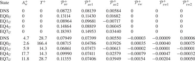
Table 3 lists the values of the energy production terms defined in (3.7) for the upper-branch equilibrium solutions and DNS with/without some suitable spanwise wall oscillations. For all uncontrolled cases,  $\mathcal {P}^{+}_{uv2}$ is very small compared to
 $\mathcal {P}^{+}_{uv1}$, indicating that the key production mechanism lies in the lift-up effect of streaks. When the control is applied, turbulence production of all upper-branch solutions and DNS exhibits a significant reduction. In particular, the reduction in the production appears dominantly in
 $\mathcal {P}^{+}_{uv1}$, except for EQ4
 $_U$, which exhibits a significant reduction in
 $\mathcal {P}^{+}_{uv2}$. This suggests that the central mechanism of the stabilisation of the ECS and turbulence is presumably the inhibition of the lift-up effect of streaks by the spanwise wall oscillation, consistent with the observation in § 3.3 where the drag reduction mechanism was proposed in terms of enhanced mixing between low- and high-speed streaky flow regions by the Stokes layer. This also explains why many previous linear analyses (Duque-Daza et al. Reference Duque-Daza, Baig, Lockerby, Chernyshenko and Davies2012; Moarref & Jovanović Reference Moarref and Jovanović2012; Blesbois et al. Reference Blesbois, Chernyshenko, Touber and Leschziner2013; Hack & Zaki Reference Hack and Zaki2015) have been so successful for a sound description of turbulence suppression and drag reduction by spanwise wall oscillation – one of the main effects that can be quantified by the linear analyses mentioned above is the amplification strength of the streaks by the streamwise vortices (i.e. the lift-up effect). The analysis here also suggests that the nonlinear mechanisms are relatively less important, and they appear to play relatively limited roles in the suppression of turbulence.
The time-averaged rate of productions of TKE with and without spanwise wall oscillation. For further details, see (3.7).

4. Conclusion
A set of exact coherent states was investigated subject to spanwise wall oscillation. Generally, the upper branches of the solutions are found to be stabilised significantly by the wall oscillation, whereas the lower branches are affected only modestly. The significantly stabilised upper-branch solutions lead the saddle–node bifurcation point of the solutions to higher Reynolds numbers, although such a trend is reversed at least for EQ0 when  ${T^{+}} \gtrsim 100$, consistent with the observation in previous DNS studies. The exact coherent states reproduce the typical streak variation behaviours observed in previous numerical and experimental work, and unveil the rich dynamics of coherent structures under the spanwise wall oscillation. In particular, it was observed that the Stokes layer enhances the fluid mixing between the low- and high-speed streaks, such that the two streaks become more symmetric with each other and subsequently weaken the wall-normal gradient of the streamwise velocity (i.e. skin friction). Visualisation of some physically relevant state portraits shows that the size of the state space supporting the turbulent state is reduced by the spanwise wall oscillation, while the upper-branch equilibrium states become less repelling, with many of their unstable eigenmodes being stabilised. The change in the state space dynamics leads to a significant reduction in lifetime of turbulence. Finally, the main stabilisation mechanism of exact coherent states is the suppression of the lift-up effect, and this explains well why many previous linear analyses have been so successful for stabilisation of turbulence and the resulting drag reduction.
Together with previous studies on exact coherent states under flow controls (Stone et al. Reference Stone, Waleffe and Graham2002, Reference Stone, Roy, Larson, Waleffe and Graham2004; Li et al. Reference Li, Xi and Graham2006; Li & Graham Reference Li and Graham2007; Ibrahim et al. Reference Ibrahim, Yang, Doohan and Hwang2019; Davis & Park Reference Davis and Park2020), the present study suggests that the drag reduction mechanism is linked closely to stabilisation of turbulence. Although the controls often have a very modest effect on the lower-branch solutions, they stabilise strongly the upper-branch solutions mainly supporting the turbulent state. This leads to an increase of the critical Reynolds number for the saddle–node bifurcation of the exact coherent states, consistent with the increased size of the basin of attraction of the laminar state reported by Rabin et al. (Reference Rabin, Caulfield and Kerswell2014), and it is associated strongly with reductions in the number of unstable directions and their repelling strength, as well as a reduction in the lifetime of turbulence emerging in the form of a chaotic saddle. In particular, the increase of the Reynolds number of the saddle–node bifurcation point implies that the distance of the upper-branch states and turbulent solution from the lower-branch states and edge state would be reduced by the application of a given control. Therefore, a turbulent state subject to a successful flow control would approach some lower-branch states and the edge state in the state space, explaining the observation by Kushwaha (Reference Kushwaha2017), who reported that turbulence subject to the spanwise wall oscillation appears to stay around a (uncontrolled) lower-branch solution.
Finally, it is worth mentioning that the present study on the exact coherent states under spanwise wall oscillation is valid at low Reynolds numbers. However, given that the near-wall cycle involving the self-sustaining process is known to be statistically and dynamically universal at higher Reynolds numbers (Jiménez & Pinelli Reference Jiménez and Pinelli1999; Hwang Reference Hwang2013), the present study would also be relevant to the near-wall region at high Reynolds numbers. Nevertheless, it is important to note that as the Reynolds number is increased, the structures in the logarithmic and outer regions contribute increasingly to the near-wall skin friction (Hwang Reference Hwang2013; de Giovanetti, Hwang & Choi Reference de Giovanetti, Hwang and Choi2016). Therefore, any flow control strategies targeting the near-wall structures are expected to exhibit a performance deterioration on increasing the Reynolds number, and the spanwise wall oscillation for the near-wall structures is not an exception to this (Hurst et al. Reference Hurst, Yang and Chung2014; Gatti & Quadrio Reference Gatti and Quadrio2016; Yao, Chen & Hussain Reference Yao, Chen and Hussain2019; Marusic et al. Reference Marusic, Chandran, Rouhi, Fu, Wine, Holloway, Chung and Smits2021). In this respect, an interesting variant of the spanwise wall oscillation has been proposed recently by Marusic et al. (Reference Marusic, Chandran, Rouhi, Fu, Wine, Holloway, Chung and Smits2021), who obtained a considerable amount of skin-friction reduction with net energy savings by applying a spanwise wall oscillation for large-scale outer structures at high Reynolds numbers. This new finding is certainly beyond the analysis of the present study, although a suitable extension of the dynamical systems approach to such high Reynolds numbers may enable one to analyse the dynamics associated with the drag reduction mechanism (Hwang et al. Reference Hwang, Willis and Cossu2016; Yang et al. Reference Yang, Willis and Hwang2019; Yang & Hwang Reference Yang and Hwang2019). The effort of extending the concepts from the dynamical systems to high-Reynolds-number turbulence is an issue of ongoing investigation.
Supplementary movies
Supplementary movies are available at https://doi.org/10.1017/jfm.2022.606.
Acknowledgements
We are grateful to Prof M. Graham who shared the PhD thesis of Kushwaha (Reference Kushwaha2017) with us. Q.Y. would like to thank Prof Y.M. Chung for useful discussions.
Funding
Y.B. and Y.H. acknowledge the support of the Engineering and Physical Sciences Research Council (EPSRC; EP/T009365/1) in the UK. Q.Y. acknowledges the Natural Science Foundation of China (92052301; 11802322) and the National Numerical Windtunnel (NNW) project.
Declaration of interests
The authors report no conflict of interest.
Appendix A. Validation
In this appendix we present the validation of the code used in this study against the literature. We also present the effect of the spatial resolution on the EQ7 equilibrium solution. Figure 14 shows the mean velocity profile of the uncontrolled DNS simulation at  $Re=400$ compared to that of the classical study of Kawahara & Kida (Reference Kawahara and Kida2001) at the same parameters. We observe that our mean velocity profile matches perfectly that of Kawahara & Kida (Reference Kawahara and Kida2001). Moreover, the discretisation error of the EQ7 equilibrium solution to the grid resolution is less than
 $0.2\,\%$, as shown in table 4.
The mean velocity profile of the uncontrolled full DNS simulation at  $Re=400$ with
 $(N_x, N_y, N_z)=(36, 61, 64)$, compared to that of Kawahara & Kida (Reference Kawahara and Kida2001).

Effect of streamwise, spanwise and wall-normal grid resolution on  $Re_{\tau }$ at
 $Re=802.2$ for EQ7 at
 ${A_w^{+}}=23.6$ and
 ${T^{+}}=28.7$.

Appendix B. Statistics for other exact coherent states
To verify that the statistics observation for EQ0 shown in figure 7 is generic, we show further the r.m.s. profiles for the equilibrium states computed in the domain  $\varOmega _{HKW}$. Figure 15 shows the r.m.s. velocity profile comparison between the controlled and uncontrolled cases for EQ1, EQ4 and EQ7. Similarly to EQ0 in figure 7, the r.m.s. profiles of the upper-branch solutions with spanwise wall oscillation become closer to those of the lower-branch solutions, which exhibit modest change by the oscillation.
Root-mean-square (r.m.s.) velocity profiles scaled with viscous inner units of the uncontrolled DNS: (a–c)  $u_{rms}^{+}$, (d–f)
 $v_{rms}^{+}$, and (g–i)
 $-\overline {u^{\prime }v^{\prime }}^{+}$. The blue and red lines indicate the controlled and uncontrolled cases, respectively. Blue solid lines: fully developed state at
 ${A_w^{+}} = 4.7$ and
 ${T^{+}}=28.7$. Upper branches are shown with dash-dotted lines, and lower branches with dashed lines: (a,d,g) EQ1 with
 ${A_w^{+}}=5.9$,
 ${T^{+}}=14.3$; (b,e,h) EQ4 with
 ${A_w^{+}}=17.7$,
 ${T^{+}}=14.3$; (c, f,i) EQ7 with
 ${A_w^{+}}=11.8$,
 ${T^{+}}=28.7$.