1 Introduction
The flutter of the skin panels of flight vehicles is a dangerous phenomenon leading to high-amplitude vibrations of panels, their fatigue and possible failure. From a theoretical point of view, the problem lies in the instability of elastic plates or shells moving in air (or being in air) with supersonic speeds. As a rule, uniform air flow over the plate is considered, and the boundary layer is neglected. Intensive studies of this problem were conducted in the 1950s–1970s and summarised in reviews by Bolotin (Reference Bolotin1963), Dowell (Reference Dowell1974) and Novichkov (Reference Novichkov1978). During the last decade, renewed interest in panel flutter has arisen due to new computational techniques devoted to nonlinear limit-cycle oscillations (Mei et al. Reference Mei, Abdel-Motagaly and Chen1999), use of new materials for skin panels (Zhou et al. Reference Zhou, Lai, Xue, Huang and Mei1995; Duan et al. Reference Duan, Abdel-Motagaly, Guo and Mei2003) and unsteady aerodynamic models suitable for transonic and low supersonic flight conditions (Bendiksen & Davis Reference Bendiksen and Davis1995; Gordnier & Visbal Reference Gordnier and Visbal2002; Vedeneev Reference Vedeneev2012, Reference Vedeneev2013a ; Shishaeva et al. Reference Shishaeva, Vedeneev and Aksenov2015).
While the stability of elastic panels in uniform flows has been studied more or less in detail, the effect of the boundary layer still remains an open question. The only experimental studies by Muhlstein et al. (Reference Muhlstein, Gaspers and Riddle1968) and Gaspers et al. (Reference Gaspers, Muhlstein and Petroff1970) devoted specifically to the boundary layer influence on panel flutter showed that it has a stabilising effect, namely, critical dynamic pressure increases when the boundary layer is thicker. Theoretical studies (Miles Reference Miles1959; Dowell Reference Dowell1971, Reference Dowell1973; Hashimoto et al.
Reference Hashimoto, Aoyama and Nakamura2009; Visbal Reference Visbal2014; Alder Reference Alder2015, Reference Alder2016) were devoted to panel flutter in the presence of the boundary layer with the (
 $1/7$
)th-power velocity law (or similar), representing a typical turbulent boundary layer profile. However, two common shortcomings of those papers can be pointed out. First, the boundary layer profile for arbitrary flow conditions and panel locations can essentially differ from the (
 $1/7$
)th-power law. Second, panel flutter can occur in two distinct forms, coupled-mode and single-mode flutter (Vedeneev Reference Vedeneev2012). They have different physical mechanisms, so that their responses to the presence of the boundary layer are also different. It is also known that nonlinear development of single-mode and coupled-mode flutter yields different types of limit-cycle oscillations (Vedeneev Reference Vedeneev2007, Reference Vedeneev2013c
; Shishaeva et al.
Reference Shishaeva, Vedeneev and Aksenov2015). In the studies cited above, flutter type was not distinguished, so it is not clear which one was examined for boundary layer effect.
Recently, Vedeneev (Reference Vedeneev2013b
) performed asymptotic analysis of the problem for long plates in an inviscid shear layer with supersonic mean flow, when the plate length
 $L\rightarrow \infty$
and the Reynolds number
 $Re\rightarrow \infty$
. He showed that the action of the boundary layer on the coupled-mode flutter of a plate is as follows. It has a stabilising effect in the case of a flutter, i.e. the growth rate of the fluttering mode decreases, but it destabilises the plate in the case of stability in uniform flow. The action of the boundary layer on a single-mode flutter is more complex and depends on the boundary layer profile. Eigenmodes of the plate are split into two groups, supersonic and subsonic modes, which exhibit different behaviours due to the presence of the boundary layer. Namely, for generalised convex boundary layer profiles, supersonic modes are stabilised (growth rates decrease), while subsonic modes are destabilised. Instability of subsonic eigenmodes due to the boundary layer is similar to the destabilising effect of the boundary layer found by Miles (Reference Miles2001) in an incompressible fluid. For profiles with a generalised inflection point, supersonic modes are destabilised for small boundary layer thickness
 $\unicode[STIX]{x1D6FF}$
and stabilised for large thickness
 $\unicode[STIX]{x1D6FF}$
, while subsonic modes are damped.
To analyse the problem, Vedeneev (Reference Vedeneev2013b
) used the global instability criterion of Kulikovskii (Reference Kulikovskii1966) and reduced the problem to the behaviour of waves in an infinite plate. Since the coupled-mode flutter of a finite-length plate is governed by long waves with wavenumber
 $k\sim \unicode[STIX]{x1D707}^{1/3}$
, where
 $\unicode[STIX]{x1D707}$
is the ratio of the flow density to the plate material density and considered as a small parameter, he used the first term of the Heisenberg expansion for solving the Rayleigh equation. The same expansion was used for the analysis of single-mode flutter, which is governed by short waves,
 $k\gg \unicode[STIX]{x1D707}^{1/3}$
. However, first-term Heisenberg expansion can be used only for
 $k\ll 1/\unicode[STIX]{x1D6FF}$
, so the results obtained for single-mode flutter are valid only for small boundary layer thickness
 $\unicode[STIX]{x1D6FF}$
.
In this paper, we re-examine the action of the boundary layer on single-mode flutter and remove the limit of small
 $\unicode[STIX]{x1D6FF}$
by using the numerical solutions of the Rayleigh equation. In § 2, we describe the formulation of the problem. In § 3, we prove that plate waves travelling upstream are damped, and the waves travelling downstream faster than the free-stream flow are either neutral or damped. The rest of the paper is devoted to waves travelling downstream that are slower than the free-stream flow, since they and only they can result in instability. In § 4, we discuss the closed-form solution of Vedeneev (Reference Vedeneev2013b
) and its limitation and describe a numerical method for solving the Rayleigh equation and dispersion relation. Section 5 is devoted to an analysis of waves in infinite plates and the comparison of growth rates obtained through first-term Heisenberg expansion and the numerical solution of the full Rayleigh equation. Finally, in § 6, we investigate the effect of the boundary layer on single-mode flutter of finite plates.
2 Formulation of the problem and the dispersion relation
We consider the stability of an elastic plate in a shear gas flow (figure 1). The flow represents the boundary layer over the plate surface, and its undisturbed velocity and temperature profiles,
 $u_{0}(z)$
and
 $T_{0}(z)$
, respectively, are given. The problem is investigated in a two-dimensional formulation (all variables do not depend on
 $y$
); also, we neglect the growth of the boundary layer so that the unperturbed flow does not depend on
 $x$
. All variables are assumed to be non-dimensional, with the speed of sound and temperature of the flow outside the boundary layer taken as the velocity and temperature scales, the plate thickness as the length scale, and plate material density as the density scale.
Gas flow over an elastic plate.

The plate motion is governed by the Kirchhoff–Love small-deflection plate theory. In a dimensionless form, the plate equation is as follows:
 $$\begin{eqnarray}\displaystyle D\frac{\unicode[STIX]{x2202}^{4}w}{\unicode[STIX]{x2202}x^{4}}-M_{w}^{2}\frac{\unicode[STIX]{x2202}^{2}w}{\unicode[STIX]{x2202}x^{2}}+\frac{\unicode[STIX]{x2202}^{2}w}{\unicode[STIX]{x2202}t^{2}}+p(x,0,t)=0, & & \displaystyle\end{eqnarray}$$
where
 $w(x,t)$
is the plate deflection,
 $D$
is the dimensionless plate stiffness,
 $M_{w}$
is the square root of the dimensionless in-plane tension force, and
 $p(x,z,t)$
is the flow pressure disturbance induced by the plate motion, such that
 $p$
is a function of
 $w$
.
Let us consider a plate of infinite length (finite plates will be studied in § 6). Since neither plate nor flow properties depend on
 $x$
, this admits perturbations of a travelling-wave type that govern the stability of the system. Let
 $w(x,t)=\text{e}^{\text{i}(kx-\unicode[STIX]{x1D714}t)}$
and
 $p(x,z,t)=p(z)\text{e}^{\text{i}(kx-\unicode[STIX]{x1D714}t)}$
be the perturbations of the plate deflection and the flow pressure (note that, due to the linearity of the stability problem, we may assume the deflection amplitude to be unity). Substitution into (2.1) yields the dispersion relation
 $$\begin{eqnarray}\mathscr{D}(k,\unicode[STIX]{x1D714})=Dk^{4}+M_{w}^{2}k^{2}-\unicode[STIX]{x1D714}^{2}+p(0)=0.\end{eqnarray}$$
Since the pressure
 $p(0)$
is induced by the plate, we need to express it through the plate deflection to obtain a closed dispersion relation.
To calculate the pressure perturbation, we assume that the flow viscosity is essential only in the formation of the steady boundary layer as a non-uniform distribution of velocity and temperature, but the flow perturbations are considered inviscid. Namely, we neglect the viscous and temperature perturbations of the boundary layer, assuming that the Reynolds number
 $Re\rightarrow \infty$
in the equations for perturbations. These equations are then converted into the inviscid Rayleigh equation (Lees & Lin Reference Lees and Lin1946). This assumption is suitable for laminar boundary layers at high Reynolds numbers, which are observed in experiments up to
 $Re\sim 10^{5}$
for the Reynolds number based on the boundary layer thickness (Gaponov & Maslov Reference Gaponov and Maslov1980). In the case of turbulent boundary layers, this assumption can be used as the first approximation if the characteristic frequencies of the turbulent fluctuations are much higher than the frequency of growing plate oscillations.
Let
 $v(z)\text{e}^{\text{i}(kx-\unicode[STIX]{x1D714}t)}$
be the perturbation of the vertical flow velocity component. Then, the compressible Rayleigh equation (Lees & Lin Reference Lees and Lin1946) takes the following form:
 $$\begin{eqnarray}\displaystyle \frac{\text{d}}{\text{d}z}\!\left(\frac{(u_{0}-c)\,\text{d}v/\text{d}z-v\,\text{d}u_{0}/\text{d}z}{T_{0}-(u_{0}-c)^{2}}\right)-\frac{1}{T_{0}}k^{2}(u_{0}-c)v=0, & & \displaystyle\end{eqnarray}$$
where
 $c=\unicode[STIX]{x1D714}/k$
is the phase speed of the wave. When
 $v(z)$
is found, the amplitude of the pressure perturbation is expressed through
 $v(z)$
as follows:
 $$\begin{eqnarray}\displaystyle p(z)=\frac{\unicode[STIX]{x1D707}}{\text{i}k}\frac{(u_{0}-c)\,\text{d}v/\text{d}z-v\,\text{d}u_{0}/\text{d}z}{T_{0}-(u_{0}-c)^{2}}, & & \displaystyle\end{eqnarray}$$
where
 $\unicode[STIX]{x1D707}$
is the dimensionless density of the flow outside the boundary layer. We will assume that
 $\unicode[STIX]{x1D707}$
is a small parameter, as, for all solid material plates and flow conditions available in applications, it has an order of
 $0.001$
or less.
The boundary conditions for the Rayleigh equation are as follows. First, at the plate surface
 $z=0$
, the impenetrability condition must be satisfied. Since the plate shape is
 $w(x)=\text{e}^{\text{i}(kx-\unicode[STIX]{x1D714}t)}$
, we obtain
 $$\begin{eqnarray}\displaystyle v(0)=\frac{\unicode[STIX]{x2202}w}{\unicode[STIX]{x2202}t}+u_{0}(0)\frac{\unicode[STIX]{x2202}w}{\unicode[STIX]{x2202}x}=-\text{i}\unicode[STIX]{x1D714},\quad z=0. & & \displaystyle\end{eqnarray}$$
Second, the radiation condition must be satisfied as
 $z\rightarrow +\infty$
. We will assume that the flow profile outside the boundary layer is constant, i.e.
 $u_{0}\equiv M$
, and
 $T_{0}\equiv 1$
for
 $z>\unicode[STIX]{x1D6FF}$
, where
 $M>1$
is the free-stream Mach number. This admits transference of the radiation condition from infinity to
 $z=\unicode[STIX]{x1D6FF}$
in the following way. For
 $z>\unicode[STIX]{x1D6FF}$
, the Rayleigh equation (2.3) is an equation with constant coefficients. Its solution satisfying the radiation condition is an exponent
 $v(z)=C\text{e}^{\unicode[STIX]{x1D6FE}z}$
,
 $\unicode[STIX]{x1D6FE}=-\sqrt{k^{2}-(M_{\infty }k-\unicode[STIX]{x1D714})^{2}}$
, where the square root branch is chosen so that
 $\text{Re}\,\unicode[STIX]{x1D6FE}<0$
for
 $\text{Im}\,\unicode[STIX]{x1D714}\gg 1$
. At
 $z=\unicode[STIX]{x1D6FF}$
, this solution must be matched with the solution inside the boundary layer. The matching condition is
 $$\begin{eqnarray}\displaystyle v(z)=C\text{e}^{\unicode[STIX]{x1D6FE}z},\quad \frac{\text{d}v(z)}{\text{d}z}=C\unicode[STIX]{x1D6FE}\text{e}^{\unicode[STIX]{x1D6FE}z},\quad z=\unicode[STIX]{x1D6FF}, & & \displaystyle\end{eqnarray}$$
which after excluding
 $C$
transforms to
 $$\begin{eqnarray}\displaystyle \frac{1}{v}\frac{\text{d}v}{\text{d}z}=\unicode[STIX]{x1D6FE},\quad z=\unicode[STIX]{x1D6FF}. & & \displaystyle\end{eqnarray}$$
Thus, to calculate the pressure
 $p(0)$
in (2.2), we have to solve the Rayleigh equation (2.3) with boundary conditions (2.5) and (2.7), and then use the expression (2.4).
Collecting all the assumptions made throughout this section, we
-
(1) investigate the problem in 2D formulation, neglecting the growth of the boundary layer,
-
(2) neglect viscous and temperature perturbations of the boundary layer (
 $Re\rightarrow \infty$
), and use the inviscid compressible Rayleigh equation,
-
(3) assume that the flow outside the boundary layer is uniform, and assign the second boundary condition for the Rayleigh equation at
$z=\unicode[STIX]{x1D6FF}$
(not at
$z=\infty$
), and -
(4) consider the dimensionless density of the flow outside the boundary layer
$\unicode[STIX]{x1D707}$
as a small parameter, which is suitable for most applications.


When
 $\unicode[STIX]{x1D707}=0$
, i.e. the flow is absent, solutions
 $\unicode[STIX]{x1D714}(k)$
of the dispersion relation (2.2) are real and correspond to bending plate waves. If
 $\unicode[STIX]{x1D707}\not =0$
, but
 $\unicode[STIX]{x1D6FF}=0$
, i.e. the flow is uniform, the downstream-travelling wave is growing for
 $0<\text{Re}\,c<M-1$
, neutral for
 $M-1<\text{Re}\,c<M+1$
and damped for
 $\text{Re}\,c>M+1$
(Vedeneev Reference Vedeneev2005). The thresholds
 $$\begin{eqnarray}\displaystyle \text{Re}\,c=M\pm 1\quad \Longleftrightarrow \quad k_{M\pm 1}=\sqrt{\frac{(M\pm 1)^{2}-M_{w}^{2}}{D}} & & \displaystyle\end{eqnarray}$$
correspond to waves travelling with the speed of the acoustic perturbations of the flow. Upstream-travelling waves,
 $\text{Re}\,c<0$
, are always damped. Now, let us consider the influence of the shear layer, i.e. assume that
 $\unicode[STIX]{x1D6FF}\not =0$
.
3 Waves with phase speed
$\text{Re}\,c>M$
or
$\text{Re}\,c<0$


In this section, we analytically prove that waves of phase speeds
 $\text{Re}\,c>M$
or
 $\text{Re}\,c<0$
are either neutral or damped so that they cannot result in instability. This was proved by Vedeneev (Reference Vedeneev2013b
) using long-wave expansion for the solutions of the Rayleigh equation (2.3), i.e. that proof is valid for wavelengths
 $\unicode[STIX]{x1D706}\gg \unicode[STIX]{x1D6FF}$
. In this section, we prove this for arbitrary wavelengths. The other case,
 $0<\text{Re}\,c<M$
, is studied numerically in the next sections.
3.1 Case
$M<\text{Re}\,c<M+1$

For neutral waves with real phase speeds
 $M<c<M+1$
, the flow does not have a critical point
 $z_{c}$
(i.e. the point where
 $u_{0}(z_{c})=c$
), and solutions of the Rayleigh equation (2.3) are regular. Also,
 $\unicode[STIX]{x1D6FE}\in \mathbb{R}$
in the boundary condition (2.7). Substitution
 $v(z)=\text{i}\tilde{v}(z)$
results in a real boundary condition for
 $\tilde{v}(z)$
:
 $$\begin{eqnarray}\displaystyle \tilde{v}(0)=-\unicode[STIX]{x1D714},\quad z=0,\quad \frac{1}{\tilde{v}}\frac{\text{d}\tilde{v}}{\text{d}z}=\unicode[STIX]{x1D6FE},\quad z=\unicode[STIX]{x1D6FF}. & & \displaystyle\end{eqnarray}$$
Since
 $\tilde{v}(z)$
also satisfies the Rayleigh equation, which is regular, we conclude that
 $\tilde{v}(z)\in \mathbb{R}$
. This means that the pressure (2.4)
 $p(z)\in \mathbb{R}$
.
As
 $\unicode[STIX]{x1D707}$
is a small parameter,
 $p(0)$
gives a small real correction for the solution of (2.2). Namely, using Taylor expansion, we obtain
 $$\begin{eqnarray}\displaystyle \hspace{-15.00002pt}\unicode[STIX]{x1D714}(k,\unicode[STIX]{x1D707})=\unicode[STIX]{x1D714}(k,0)+\unicode[STIX]{x1D707}\!\left.\frac{\unicode[STIX]{x2202}\unicode[STIX]{x1D714}}{\unicode[STIX]{x2202}\unicode[STIX]{x1D707}}\right|_{\unicode[STIX]{x1D707}=0}+o(\unicode[STIX]{x1D707}) & = & \displaystyle \unicode[STIX]{x1D714}(k,0)-\unicode[STIX]{x1D707}\frac{\unicode[STIX]{x2202}\mathscr{D}}{\unicode[STIX]{x2202}\unicode[STIX]{x1D707}}\left/\frac{\unicode[STIX]{x2202}\mathscr{D}}{\unicode[STIX]{x2202}\unicode[STIX]{x1D714}}\right|_{\unicode[STIX]{x1D707}=0}+o(\unicode[STIX]{x1D707})\nonumber\\ \displaystyle & = & \displaystyle \unicode[STIX]{x1D714}(k,0)+\frac{\unicode[STIX]{x1D707}}{2\unicode[STIX]{x1D714}(k,0)}\!\left.\frac{\unicode[STIX]{x2202}p(0)}{\unicode[STIX]{x2202}\unicode[STIX]{x1D707}}\right|_{\unicode[STIX]{x1D707}=0}+o(\unicode[STIX]{x1D707}).\end{eqnarray}$$
We conclude that
 $\unicode[STIX]{x1D714}(k,\unicode[STIX]{x1D707})$
is real, i.e. the wave stays neutral in the presence of the boundary layer.
3.2 Case
$\text{Re}\,c>M+1$

In this case, for real
 $c$
, there is also no critical point, so that the solutions of the Rayleigh equation (2.3) are regular, but
 $\unicode[STIX]{x1D6FE}$
is now purely imaginary (namely,
 $\unicode[STIX]{x1D6FE}=\text{i}\tilde{\unicode[STIX]{x1D6FE}}$
,
 $\tilde{\unicode[STIX]{x1D6FE}}>0$
), i.e.
 $p(0)\not \in \mathbb{R}$
, and, as can be seen from (3.2),
 $\unicode[STIX]{x1D714}(k,\unicode[STIX]{x1D707})\not \in \mathbb{R}$
. Let us prove that
 $\text{Im}\,\unicode[STIX]{x1D714}(k,\unicode[STIX]{x1D707})<0$
, i.e. the wave is damped. Using (3.2), it is sufficient to prove that
 $\text{Im}\,p(0)<0$
.
We will study two cases. The first is a non-zero denominator in (2.3), i.e.
 $T_{0}(z)-(u_{0}(z)-c)^{2}\not =0$
,
 $0\leqslant z\leqslant \unicode[STIX]{x1D6FF}$
. This means that the Rayleigh equation is regular. The other case is the existence of a point
 $z_{a}$
where
 $T_{0}(z_{a})-(u_{0}(z_{a})-c)^{2}=0$
. This point is a removable singularity of the Rayleigh equation (Lees & Lin Reference Lees and Lin1946).
Let us assume the first case. Consider two real linearly independent solutions
 $v_{1}(z)$
and
 $v_{2}(z)$
of (2.3), satisfying conditions
 $$\begin{eqnarray}\displaystyle v_{1}(0)=1,\quad v_{1}^{\prime }(0)=0,\quad v_{2}(0)=0,\quad v_{2}^{\prime }(0)=1. & & \displaystyle\end{eqnarray}$$
Then the general solution can be expressed as
 $$\begin{eqnarray}\displaystyle v(z)=c_{1}v_{1}(z)+c_{2}v_{2}(z). & & \displaystyle\end{eqnarray}$$
Satisfying (2.5) and (2.7), we obtain
 $$\begin{eqnarray}\displaystyle c_{1}=-\text{i}\unicode[STIX]{x1D714},\quad c_{2}=\text{i}\unicode[STIX]{x1D714}\frac{\unicode[STIX]{x1D6FE}v_{1}(\unicode[STIX]{x1D6FF})-v_{1}^{\prime }(\unicode[STIX]{x1D6FF})}{\unicode[STIX]{x1D6FE}v_{2}(\unicode[STIX]{x1D6FF})-v_{2}^{\prime }(\unicode[STIX]{x1D6FF})}. & & \displaystyle\end{eqnarray}$$
Now consider pressure
 $$\begin{eqnarray}\displaystyle p(z)=c_{1}p_{1}(z)+c_{2}p_{2}(z), & & \displaystyle\end{eqnarray}$$
where
 $p_{j}$
and
 $v_{j}$
are connected through (2.4). Since
 $c_{1}$
is purely imaginary, and
 $v_{1}$
is real, we conclude that
 $c_{1}p_{1}(z)\in \mathbb{R}$
. Then
 $$\begin{eqnarray}\displaystyle \text{Im}\,p(0)=\text{Im}(c_{2}p_{2}(0)). & & \displaystyle\end{eqnarray}$$
Using (2.4) gives
 $$\begin{eqnarray}\displaystyle p_{2}(0)=\frac{\unicode[STIX]{x1D707}}{\text{i}k}\frac{-c}{T_{0}(0)-c^{2}}=\text{i}P,\quad P<0, & & \displaystyle\end{eqnarray}$$
where the last inequality is obtained by assuming that the denominator
 $T_{0}(z)-(u_{0}(z)-c)^{2}\not =0$
, and taking into account that, at
 $z=\unicode[STIX]{x1D6FF}$
, it equals
 $1-(M-c)^{2}<0$
.
Finally, using (3.5b ) and (3.8), we obtain
 $$\begin{eqnarray}\displaystyle \text{Im}\,p(0) & = & \displaystyle \text{Im}\!\left(-P\unicode[STIX]{x1D714}\frac{\text{i}\tilde{\unicode[STIX]{x1D6FE}}v_{1}(\unicode[STIX]{x1D6FF})-v_{1}^{\prime }(\unicode[STIX]{x1D6FF})}{\text{i}\tilde{\unicode[STIX]{x1D6FE}}v_{2}(\unicode[STIX]{x1D6FF})-v_{2}^{\prime }(\unicode[STIX]{x1D6FF})}\right)\nonumber\\ \displaystyle & = & \displaystyle \text{Im}\!\left(-P\unicode[STIX]{x1D714}\frac{(\text{i}\tilde{\unicode[STIX]{x1D6FE}}v_{1}(\unicode[STIX]{x1D6FF})-v_{1}^{\prime }(\unicode[STIX]{x1D6FF}))(-\text{i}\tilde{\unicode[STIX]{x1D6FE}}v_{2}(\unicode[STIX]{x1D6FF})-v_{2}^{\prime }(\unicode[STIX]{x1D6FF}))}{\tilde{\unicode[STIX]{x1D6FE}}^{2}v_{2}^{2}(\unicode[STIX]{x1D6FF})+v_{2}^{\prime 2}(\unicode[STIX]{x1D6FF})}\right)\nonumber\\ \displaystyle & = & \displaystyle P\unicode[STIX]{x1D714}\tilde{\unicode[STIX]{x1D6FE}}\frac{(v_{1}(\unicode[STIX]{x1D6FF})v_{2}^{\prime }(\unicode[STIX]{x1D6FF})-v_{2}(\unicode[STIX]{x1D6FF})v_{1}^{\prime }(\unicode[STIX]{x1D6FF}))}{\tilde{\unicode[STIX]{x1D6FE}}^{2}v_{2}^{2}(\unicode[STIX]{x1D6FF})+v_{2}^{\prime 2}(\unicode[STIX]{x1D6FF})}=\frac{P\unicode[STIX]{x1D714}\tilde{\unicode[STIX]{x1D6FE}}}{\tilde{\unicode[STIX]{x1D6FE}}^{2}v_{2}^{2}(\unicode[STIX]{x1D6FF})+v_{2}^{\prime 2}(\unicode[STIX]{x1D6FF})}W(v_{1},v_{2})(\unicode[STIX]{x1D6FF}).\end{eqnarray}$$
Here,
 $W(v_{1},v_{2})$
is the Wronskian of
 $v_{1}$
and
 $v_{2}$
. As
 $v_{1}$
and
 $v_{2}$
are linearly independent,
 $W(v_{1},v_{2})(z)\not =0$
for any
 $z$
. Also,
 $W(v_{1},v_{2})(0)=1$
; therefore, we conclude that
 $W(v_{1},v_{2})(\unicode[STIX]{x1D6FF})>0$
, and, finally,
 $\text{Im}\,p(0)<0$
.
Now, assume the second case, i.e. there exists a point
 $z_{a}$
such that
 $T_{0}(z_{a})-(u_{0}(z_{a})-c)^{2}=0$
. In this case,
 $P>0$
, since the denominator in (2.4) changes its sign at
 $z=z_{a}$
. Rewrite
 $W(v_{1},v_{2})$
in the following form:
 $$\begin{eqnarray}\displaystyle (u_{0}-c)W(v_{1},v_{2}) & = & \displaystyle (u_{0}-c)(v_{1}v_{2}^{\prime }-v_{2}v_{1}^{\prime })\nonumber\\ \displaystyle & = & \displaystyle ((u_{0}-c)v_{2}^{\prime }v_{1}-u_{0}^{\prime }v_{2}v_{1})-((u_{0}-c)v_{1}^{\prime }v_{2}-u_{0}^{\prime }v_{1}v_{2})\nonumber\\ \displaystyle & = & \displaystyle v_{1}((u_{0}-c)v_{2}^{\prime }-u_{0}^{\prime }v_{2})-v_{2}((u_{0}-c)v_{1}^{\prime }-u_{0}^{\prime }v_{1}).\end{eqnarray}$$
Since
 $z_{a}$
is a removable singularity, the numerator in the first term of (2.3) is zero at
 $z=z_{a}$
for both
 $v=v_{1}(z)$
and
 $v_{2}(z)$
. Hence, both terms on the right-hand side of (3.10) are zero at
 $z=z_{a}$
. As
 $u_{0}(z_{a})-c\not =0$
,
 $W(v_{1},v_{2})(z_{a})=0$
, i.e. the Wronskian changes its sign at
 $z=z_{a}$
. Given that
 $W(v_{1},v_{2})(0)=1$
, we conclude that
 $W(v_{1},v_{2})(\unicode[STIX]{x1D6FF})<0$
, and
 $\text{Im}\,p(0)<0$
, which finalises the proof of
 $\text{Im}\,\unicode[STIX]{x1D714}(k,\unicode[STIX]{x1D707})<0$
.
3.3 Case
$\text{Re}\,c<0$

The case of upstream-travelling waves is reduced to the previous case with the following changes. First,
 $\tilde{\unicode[STIX]{x1D6FE}}<0$
. Second, since
 $c$
is negative,
 $P$
changes its sign. Third,
 $\unicode[STIX]{x1D714}(k,0)<0$
, hence
 $\text{Im}\,p(0)>0$
, and, due to (3.2),
 $\text{Im}\,\unicode[STIX]{x1D714}<0$
.
Note that, for
 $k\sim \unicode[STIX]{x1D707}^{1/3}$
or less,
 $\unicode[STIX]{x1D714}(k,0)\sim \unicode[STIX]{x1D707}^{2/3}$
, and the expansion (3.2) is not valid any more since
 $p(0)$
and other terms in (2.2) are of the same order. However, in this case, we can use the long-wave expansion of the dispersion relation in the form of equation (5.7) of Vedeneev (Reference Vedeneev2013b
):
 $$\begin{eqnarray}\displaystyle Dk^{4}+M_{w}^{2}k^{2}-\unicode[STIX]{x1D714}^{2}-\frac{\unicode[STIX]{x1D707}\unicode[STIX]{x1D714}k}{\text{i}a\unicode[STIX]{x1D714}-\unicode[STIX]{x1D6FF}bk^{2}}=0,\quad a>0,\quad b>0. & & \displaystyle\end{eqnarray}$$
Assuming
 $k\in \mathbb{R}$
,
 $\unicode[STIX]{x1D714}=\unicode[STIX]{x1D714}_{r}+\text{i}\unicode[STIX]{x1D714}_{i}$
,
 $\unicode[STIX]{x1D714}_{r}<0$
, and taking the imaginary part of (3.11), we find that
 $$\begin{eqnarray}\displaystyle 2\unicode[STIX]{x1D714}_{r}\unicode[STIX]{x1D714}_{i}=\unicode[STIX]{x1D707}k\frac{a(\unicode[STIX]{x1D714}_{r}^{2}+\unicode[STIX]{x1D714}_{i}^{2})+\unicode[STIX]{x1D714}_{i}\unicode[STIX]{x1D6FF}k^{2}}{(a\unicode[STIX]{x1D714}_{i}+\unicode[STIX]{x1D6FF}bk^{2})^{2}+a\unicode[STIX]{x1D714}_{r}^{2}}. & & \displaystyle\end{eqnarray}$$
This equality is not satisfied if
 $\unicode[STIX]{x1D714}_{i}>0$
; therefore,
 $\unicode[STIX]{x1D714}_{i}=\text{Im}\,\unicode[STIX]{x1D714}<0$
.
4 Methods for solving the Rayleigh equation and dispersion relation
In the previous section, we proved that waves with phase speed
 $\text{Re}\,c<0$
or
 $\text{Re}\,c>M$
are either neutral or damped. Hence, only waves with
 $0<\text{Re}\,c<M$
can be growing. Let us now consider such waves.
We will use three approaches for solving the Rayleigh equation, finding
 $p(0)$
and then solving the dispersion relation (2.2). The first approach, which we will refer to as ‘analytical’, was used by Vedeneev (Reference Vedeneev2013b
). Though it admits general investigation of the wave behaviour, it is not valid for short waves. The second approach, which we will refer to as ‘numerical’, consists in numerical solution of both the Rayleigh equation and the dispersion relation. Obviously, it is valid for arbitrary wavelengths; we will use it for analysis of short-wave behaviour. The third, intermediate approach, which we will call ‘semi-analytical’, consists in analytical solution of the Rayleigh equation (similar to the ‘analytical’ approach), but a numerical solution of the dispersion relation. This approach will be used as a connection between analytical and numerical results.
4.1 Analytical solution for ‘short’ waves
The solution of the Rayleigh equation can be written in the form of a series in
 $k^{2}$
, known as the Heisenberg expansion (Drazin & Reid Reference Drazin and Reid2004). Vedeneev (Reference Vedeneev2013b
) considered the first term of this expansion, which is valid for
 $k\ll 1/\unicode[STIX]{x1D6FF}$
, i.e. for wavelengths that are much longer than the boundary layer thickness. Such consideration is equivalent to neglecting the second term of order
 $k^{2}$
in (2.3). When this term is omitted, (2.3) is solved in a closed form. Satisfying boundary conditions (2.5) and (2.7), he obtained the pressure in the form
 $$\begin{eqnarray}\displaystyle p(0)=-\unicode[STIX]{x1D707}\left(\left(\frac{(Mk-\unicode[STIX]{x1D714})^{2}}{\sqrt{k^{2}-(Mk-\unicode[STIX]{x1D714})^{2}}}\right)^{-1}+\unicode[STIX]{x1D6FF}\left(\displaystyle \int _{0}^{1}\displaystyle \frac{T_{0}(\unicode[STIX]{x1D702})\,\text{d}\unicode[STIX]{x1D702}}{(u_{0}(\unicode[STIX]{x1D702})-c)^{2}}-1\right)\right)^{-1}, & & \displaystyle\end{eqnarray}$$
where
 $\unicode[STIX]{x1D702}=z/\unicode[STIX]{x1D6FF}$
is the inner boundary layer coordinate, and
 $c=\unicode[STIX]{x1D714}/k$
is the phase speed. Here, the first term in parentheses represents the contribution of the uniform flow outside the boundary layer, while the second term represents the contribution of the boundary layer. Substitution in (2.2) yields the dispersion relation
 $$\begin{eqnarray}\displaystyle \hspace{-16.99998pt}\mathscr{D}(k,\unicode[STIX]{x1D714}) & = & \displaystyle (Dk^{4}+M_{w}^{2}k^{2}-\unicode[STIX]{x1D714}^{2})\nonumber\\ \displaystyle & & \displaystyle -\,\unicode[STIX]{x1D707}\left(\left(\frac{(Mk-\unicode[STIX]{x1D714})^{2}}{\sqrt{k^{2}-(Mk-\unicode[STIX]{x1D714})^{2}}}\right)^{-1}+\unicode[STIX]{x1D6FF}\left(\displaystyle \int _{0}^{1}\displaystyle \frac{T_{0}(\unicode[STIX]{x1D702})\,\text{d}\unicode[STIX]{x1D702}}{(u_{0}(\unicode[STIX]{x1D702})-c)^{2}}-1\right)\right)^{-1}=0.\end{eqnarray}$$
As
 $\unicode[STIX]{x1D6FF}\rightarrow 0$
, the dispersion relation (4.2) coincides with the dispersion relation for a plate in uniform flow (Kornecki Reference Kornecki1979; Vedeneev Reference Vedeneev2005).
A closed-form solution of the dispersion relation (4.2) can be obtained if an additional condition is satisfied: wavenumber
 $k\gg \unicode[STIX]{x1D707}^{1/3}$
, i.e. the wave is not too long. This condition means that the order of the first term in (4.2) is larger than the second, i.e. the wave is mostly governed by the plate, while the flow gives just a small correction of the order of
 $\unicode[STIX]{x1D707}$
. Under this condition, the Taylor expansion of the solution of (4.2) in
 $\unicode[STIX]{x1D707}$
gives the following (similar to (3.2)):
 $$\begin{eqnarray}\displaystyle \unicode[STIX]{x1D714}(k,\unicode[STIX]{x1D707}) & = & \displaystyle \unicode[STIX]{x1D714}(k,0)-\frac{\unicode[STIX]{x1D707}}{2\unicode[STIX]{x1D714}(k,0)}\nonumber\\ \displaystyle & & \displaystyle \times \left(\left(\frac{(M_{\infty }k-\unicode[STIX]{x1D714})^{2}}{\sqrt{k^{2}-(M_{\infty }k-\unicode[STIX]{x1D714})^{2}}}\right)^{-1}+\unicode[STIX]{x1D6FF}\left(\displaystyle \int _{0}^{1}\displaystyle \frac{T_{0}(\unicode[STIX]{x1D702})\,\text{d}\unicode[STIX]{x1D702}}{(u_{0}(\unicode[STIX]{x1D702})-c)^{2}}-1\right)\right)^{-1},\end{eqnarray}$$
where the expression in parentheses is calculated at
 $\unicode[STIX]{x1D707}=0$
. Here, the first term
 $\unicode[STIX]{x1D714}(k,0)$
is a frequency of the plate in vacuum, while the second term of order
 $\unicode[STIX]{x1D707}$
is a small frequency correction due to the flow.
Note that, for solution (4.3), both conditions
 $k\gg \unicode[STIX]{x1D707}^{1/3}$
and
 $k\ll 1/\unicode[STIX]{x1D6FF}$
must be satisfied, i.e. the wavelengths are bounded both above and below. Such waves were called ‘short’ (in quotation marks) (Vedeneev Reference Vedeneev2013b
) since they do not include shorter wavelengths,
 $k\gtrsim 1/\unicode[STIX]{x1D6FF}$
. Let us consider numerical methods for solving the Rayleigh equation and the dispersion relation, which are valid for waves of arbitrary length.
4.2 Numerical solution for arbitrary wavelengths
In order to overcome the restriction
 $k\ll 1/\unicode[STIX]{x1D6FF}$
and consider arbitrary wavelengths, we solve the Rayleigh equation numerically through the Runge–Kutta method. The difficulty associated with logarithmic singularity at the critical point is eliminated by solving the equation along a path in the complex
 $z$
-plane. Namely, the algorithm is as follows.
-
(1) For a given velocity profile
$u_{0}(z)$
, we find the critical point
$z_{c}$
as a root of the equation
$u_{0}(z)=c$
. -
(2) If the critical point exists, i.e.
$0<\text{Re}\,z_{c}<\unicode[STIX]{x1D6FF}$
, then according to Lin’s rule, this point must be passed below in the complex
$z$
-plane in order to obtain a solution that is a limit of the viscous solution as
$Re\rightarrow \infty$
(vanishing viscosity) (Drazin & Reid Reference Drazin and Reid2004). In order to enforce this rule, we choose a smooth path passing below the critical point in the complex
$z$
-plane. If
$\text{Im}\,z_{c}$
is positive and not too close to zero (namely,
$\text{Im}\,z_{c}\geqslant \unicode[STIX]{x1D6FF}/2$
), then the path is a real segment
$[0;\unicode[STIX]{x1D6FF}]$
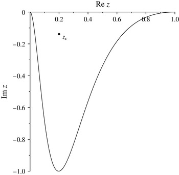
. Otherwise, the path is complex, as shown in figure 2. Note that, for small positive
$\text{Im}\,z_{c}$
, the equation can be integrated along the real segment, but we still use the complex path to avoid numerical difficulties due to the closeness of the critical point, which is a point of singularity for the Rayleigh equation. -
(3) The boundary value problem is reduced to two initial value problems by the standard shooting method. They are both solved along the chosen path through the Runge–Kutta method. The velocity perturbation
$v(z)$
and its derivative
$\text{d}v(z)/\text{d}z$
are found. -
(4) Finally, by using formula (2.4), we calculate the unsteady pressure
$p(0)$
on the plate surface.


Integration path chosen for solving the Rayleigh equation for the velocity profile
 $u_{0}(\unicode[STIX]{x1D702})=M\sin (\unicode[STIX]{x03C0}\unicode[STIX]{x1D702}/2)$
,
 $M=1.6$
and
 $c=0.5-0.33\text{i}$
. The critical point is
 $z_{c}\approx 0.20-0.14\text{i}$
,
 $\unicode[STIX]{x1D6FF}=1$
.

For solving the dispersion equation (2.2), we use the following iterative procedure. We let the wavenumber
 $k$
be given, and we search
 $\unicode[STIX]{x1D714}(k)$
, satisfying the dispersion equation. In the first step,
 $\unicode[STIX]{x1D714}_{1}$
equals the natural frequency of the plate in vacuum:
 $$\begin{eqnarray}\displaystyle \unicode[STIX]{x1D714}_{1}=\sqrt{Dk^{4}+M_{w}^{2}k^{2}}. & & \displaystyle\end{eqnarray}$$
Now, let us have
 $n$
th iteration,
 $\unicode[STIX]{x1D714}_{n}$
. We numerically solve the Rayleigh equation and calculate the unsteady pressure
 $p(0,\unicode[STIX]{x1D714}_{n})$
according to the procedure described above. Then, we put
 $$\begin{eqnarray}\displaystyle \unicode[STIX]{x1D714}_{n+1}=\sqrt{Dk^{4}+M_{w}^{2}k^{2}+p(0,\unicode[STIX]{x1D714}_{n})}. & & \displaystyle\end{eqnarray}$$
Iterations are repeated until the desired accuracy is achieved, i.e.
 $|\mathscr{D}(k,\unicode[STIX]{x1D714}_{n})|<\unicode[STIX]{x1D700}$
.
A convergence study shows that
 $N=3000$
points is enough for discretising the Rayleigh equation along the integration path to get an accurate solution through the Runge–Kutta method. For the iterative solution of the dispersion relation,
 $\unicode[STIX]{x1D700}=10^{-10}$
gives a well-converged solution
 $\unicode[STIX]{x1D714}(k)$
for all wavenumbers
 $k$
considered in the examples below.
4.3 Semi-analytical solution for ‘short’ and long waves
The analytical solution is not applicable in the case of very long waves,
 $k\sim \unicode[STIX]{x1D707}^{1/3}$
, since the expressions in the first and second parentheses in (4.2) have the same order, and the Taylor expansion (4.3) is not valid. In this paper, we are interested in the role of the second term of the Rayleigh equation, which is essential for
 $k\gtrsim 1/\unicode[STIX]{x1D6FF}$
. However, depending on the particular boundary layer profile, the latter segment can overlap the range
 $k\sim \unicode[STIX]{x1D707}^{1/3}$
, i.e. there can be no range of wavenumbers where the analytical solution is valid. In this case, instead of an analytical approach, we use a ‘semi-analytical’ approach, which consists in the following. We use the dispersion relation (4.2), i.e. neglect the second term in the Rayleigh equation. However, instead of using the Taylor expansion (4.3), the dispersion relation is solved numerically in the same manner as in the numerical approach. Frequencies
 $\unicode[STIX]{x1D714}(k)$
obtained through the semi-analytical approach are valid for
 $k\ll 1/\unicode[STIX]{x1D6FF}$
, without any restriction for small
 $k$
. Comparison of semi-analytical and numerical results will show the role of the second term in the Rayleigh equation for very short waves,
 $k\gtrsim 1/\unicode[STIX]{x1D6FF}$
.
5 Results: waves in an infinite plate
Since the cases of waves with
 $\text{Re}\,c>M$
and
 $\text{Re}\,c<0$
are already excluded from possibly unstable waves (§ 3), we restrict our analysis to the waves with phase speeds
 $0<\text{Re}\,c<M$
.
5.1 Generalised convex boundary layer profiles
We will call the boundary layer profile with
 $(u_{0}^{\prime }/T_{0})^{\prime }<0$
for
 $z\in [0;\unicode[STIX]{x1D6FF}]$
the generalised convex profile. Analysing a solution (4.3), Vedeneev (Reference Vedeneev2013b
) proved that, for such profiles, the action of the boundary layer on the wave is as follows.
-
(1) If the wave is growing for
$\unicode[STIX]{x1D6FF}=0$
(i.e.
$0<\text{Re}\,c<M-1$
, the wave is supersonic with respect to the mean flow), then it stays growing for
$\unicode[STIX]{x1D6FF}\not =0$
, but the growth rate monotonically decreases towards zero when
$\unicode[STIX]{x1D6FF}$
increases. -
(2) If the wave is neutral for
$\unicode[STIX]{x1D6FF}=0$
(i.e.
$M-1<\text{Re}\,c<M$
, the wave is subsonic with respect to the mean flow), then for
$\unicode[STIX]{x1D6FF}\not =0$
it starts growing. When
$\unicode[STIX]{x1D6FF}$
increases, the growth rate first increases, achieves its maximum at
$\unicode[STIX]{x1D6FF}=\unicode[STIX]{x1D6FF}_{m}$
and then monotonically decreases towards zero.







These results were obtained with the second term in the Rayleigh equation neglected, i.e. very short waves were not considered. Now, let us investigate the influence of this term.
Consider as an example the velocity profile
 $$\begin{eqnarray}\displaystyle u_{0}(z)=M\sin \!\left(\frac{\unicode[STIX]{x03C0}}{2}\frac{z}{\unicode[STIX]{x1D6FF}}\right) & & \displaystyle\end{eqnarray}$$
for parameters
 $M=1.6$
and
 $$\begin{eqnarray}\displaystyle D=23.9,\quad M_{w}=0,\quad \unicode[STIX]{x1D707}=0.00012,\quad \unicode[STIX]{x1D6FE}=1.4, & & \displaystyle\end{eqnarray}$$
which correspond to an untensioned steel plate at 3000 m, or an aluminium plate at 11 000 m above sea level. For simplicity, in all examples hereafter, we will assume that the Prandtl number
 $Pr=1$
and the plate is heat-insulated, so that the temperature profile
 $T_{0}(u_{0})$
is given by the same expression as in an adiabatic flow (Schlichting Reference Schlichting1960):
 $$\begin{eqnarray}\displaystyle T_{0}(u_{0})=1+\frac{\unicode[STIX]{x1D6FE}-1}{2}(M^{2}-u_{0}^{2}). & & \displaystyle\end{eqnarray}$$
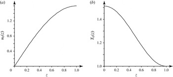
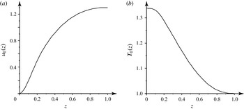
The boundary layer profile (5.1) and (5.3) is shown in figure 3.
First, let us show that this boundary layer is stable itself (i.e. over the rigid plate) in the inviscid approximation. Indeed, the stability criterion of subsonic disturbances (i.e. disturbances with the phase speed
 $c>M-1$
) is as follows (Lees & Lin Reference Lees and Lin1946): the profile must be generalised convex in the subsonic part of the layer, i.e.
 $$\begin{eqnarray}\displaystyle \left(\frac{u_{0}^{\prime }(z)}{T_{0}(z)}\right)^{\prime }<0,\quad z>z_{s}, & & \displaystyle\end{eqnarray}$$
where
 $u_{0}(z_{s})=M-1$
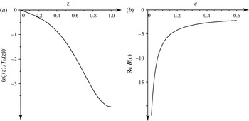
. This function is plotted in figure 4(a); clearly, the stability condition is satisfied. Next, for supersonic long-wave disturbances, Vedeneev (Reference Vedeneev2013b
) showed that the stability criterion is as follows:
 $$\begin{eqnarray}\displaystyle \text{Re}\,B(c)<0,\quad 0<c<M-1, & & \displaystyle\end{eqnarray}$$
where
 $$\begin{eqnarray}\displaystyle B(c)=\displaystyle \int _{0}^{1}\displaystyle \frac{T_{0}(\unicode[STIX]{x1D702})\,\text{d}\unicode[STIX]{x1D702}}{(u_{0}(\unicode[STIX]{x1D702})-c)^{2}}-1. & & \displaystyle\end{eqnarray}$$
It is seen in figure 4(b) that the stability condition for supersonic disturbances is also satisfied, so that the boundary layer profile (5.1) and (5.3) is indeed stable.


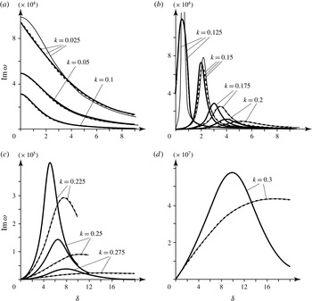
Growth rates
 $\text{Im}\,\unicode[STIX]{x1D714}(\unicode[STIX]{x1D6FF})$
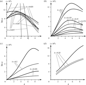
for waves that are (a) growing and (b–d) neutral in uniform flow. The boundary layer profile is given by (5.1) and (5.3). The thin continuous, dashed and thick continuous lines represent analytical, semi-analytical and numerical solutions, respectively.

Now, let us consider the influence of the second term in the Rayleigh equation on the travelling waves. Calculated growth rate versus the boundary layer thickness,
 $\text{Im}\,\unicode[STIX]{x1D714}(\unicode[STIX]{x1D6FF})$
, is plotted for a range of wavenumbers
 $k$
in figure 5. For ‘moderate’ wavelengths,
 $0.05\leqslant k\leqslant 0.1$
, there is an excellent agreement between the numerical, analytical and semi-analytical solutions. This range of wavenumbers corresponds to waves growing in uniform flow, i.e.
 $k<k_{M-1}=0.123$
(hereafter, index
 $M-1$
or
 $M$
means the value of the phase speed
 $c(k)$
for the given wavenumber). For
 $k\leqslant 0.025$
, the analytical solution shows a significant discrepancy with numerical and semi-analytical results, since the condition
 $k\gg \unicode[STIX]{x1D707}^{1/3}$
is not valid, and the Taylor expansion (4.3) cannot be used. However, the semi-analytical and numerical solutions, which do not use the Taylor expansion, are still in excellent agreement with each other.
For
 $k>0.125$
, a significant difference between numerical and analytical solutions appears due to the influence of the second term in the Rayleigh equation. The results presented in figure 5 cover the full range of
 $k_{M-1}<k<k_{M}=0.327$
and yield two corrections due to this term. First, the actual maximal growth rates are higher than predicted by analytical theory. The higher the value of
 $k$
, the higher the relative increase of
 $\max \text{Im}\,\unicode[STIX]{x1D714}(\unicode[STIX]{x1D6FF})$
due to the second term. Second, the maximum growth rate is achieved at a smaller boundary layer thickness.
We have checked several other generalised convex boundary layer profiles, including (5.1) with
 $M=1.3$
and
 $2.0$
. In all cases, the results are similar to those plotted in figure 5, and the short-wave effect of the second term in the Rayleigh equation resulted in an increase of the growth rates in all cases where this effect was visible.
We conclude that the destabilisation of neutral waves with
 $M-1<c<M$
due to the boundary layer, initially predicted by analytical theory (Vedeneev Reference Vedeneev2013b
), is confirmed by the numerical solution of the full Rayleigh equation. Moreover, the growth rates turn out to be higher than the analytical theory predicts.
5.2 Boundary layer profile with a generalised inflection point
Now, let us investigate the boundary layer profile with a generalised inflection point
 $z_{i}$
, where
 $(u_{0}^{\prime }/T_{0})^{\prime }=0$
. In subsonic flow, such a profile would be unstable, since the existence of the generalised inflection point is a necessary and sufficient condition for the inviscid instability of subsonic disturbances (Lees & Lin Reference Lees and Lin1946). However, in supersonic flow, there exist profiles such that the generalised inflection point is located in the supersonic part of the boundary layer, i.e.
 $u_{0}(z_{i})<M-1$
. This means that, on the one hand, subsonic disturbances are damped, since the criterion (5.4) is satisfied. On the other hand, supersonic disturbances can also be damped, since their stability condition (5.5) has no relation to the generalised inflection point. Consequently, such a profile can be stable and therefore can exist in real flows.
For such boundary layer profiles, studying the analytical solution, Vedeneev (Reference Vedeneev2013b ) proved that the action of the boundary layer on the wave is as follows.
-
(1) If the wave is growing for
$\unicode[STIX]{x1D6FF}=0$
(i.e.
$0<\text{Re}\,c<M-1$
), then it stays growing for
$0<\unicode[STIX]{x1D6FF}<\unicode[STIX]{x1D6FF}_{1}$
, such that the growth rate is higher than in uniform flow. For a thicker boundary layer,
$\unicode[STIX]{x1D6FF}_{1}<\unicode[STIX]{x1D6FF}<\unicode[STIX]{x1D6FF}_{2}$
, the wave is still growing, but the growth rate is lower than in uniform flow. Finally, in thick boundary layers,
$\unicode[STIX]{x1D6FF}>\unicode[STIX]{x1D6FF}_{2}$
, the wave becomes damped. -
(2) If the wave is neutral for
$\unicode[STIX]{x1D6FF}=0$
(i.e.
$M-1<\text{Re}\,c<M$
), then for
$\unicode[STIX]{x1D6FF}\not =0$
it begins to grow. The behaviour of such waves is similar to those in generalised convex boundary layers.






Let us now consider numerical results. As an example, we use the following velocity profile:
 $$\begin{eqnarray}\displaystyle u_{0}(z)=M\left(1-\left(1-\frac{z}{\unicode[STIX]{x1D6FF}}\right)^{2.4}\right)\times \cos \!\left(0.7\left(1-\frac{z}{\unicode[STIX]{x1D6FF}}\right)^{7}\right)^{7} & & \displaystyle\end{eqnarray}$$
for
 $M=1.3$
, parameters (5.2a–d
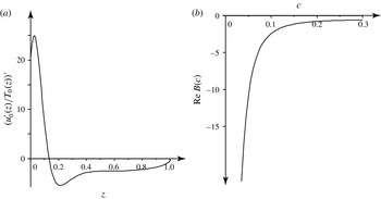
) and the temperature profile (5.3), which is shown in figure 6. Though the velocity profile (5.7) looks sophisticated, it just represents the function with one generalised inflection point located in the supersonic part of the layer. Let us show that this boundary layer is stable in inviscid approximation. First, shown in figure 7(a) is the generalised curvature
 $(u_{0}^{\prime }/T_{0})^{\prime }$
. It is negative for
 $z>z_{i}=0.133$
and
 $u_{0}(z_{i})=0.298<0.3=M-1$
, i.e. the condition (5.4) is satisfied and subsonic disturbances are damped. Second,
 $\text{Re}\,B(c)$
shown in figure 7(b) is negative for
 $c<M-1$
, i.e. the condition for supersonic disturbances (5.5) is also satisfied so that they are also damped.


As we did before, we calculated growth rates
 $\text{Im}\,\unicode[STIX]{x1D714}(\unicode[STIX]{x1D6FF})$
for a range of wavenumbers. Results for
 $k<k_{M-1}=0.061$
, which correspond to growing waves in uniform flow, are shown in figure 8(a). It is seen that there is a good agreement between the semi-analytical and numerical results. For
 $k=0.05$
, the analytical results are close, but for smaller
 $k$
they are essentially different, since
 $k\sim \unicode[STIX]{x1D707}^{1/3}$
and Taylor expansion is not applicable for such small wavenumbers. It is seen that, despite the short-wave effect not being pronounced, the growth rates obtained numerically through the full Rayleigh equation are slightly higher than those obtained in the semi-analytical approximation.
Growth rates
 $\text{Im}\,\unicode[STIX]{x1D714}(\unicode[STIX]{x1D6FF})$
for waves that are (a) growing, (b–d) neutral in uniform flow. The boundary layer profile is given by (5.3) and (5.7). The thin continuous, dashed and thick continuous lines represent the analytical, semi-analytical and numerical solutions, respectively.

For
 $k_{M-1}<k<k_{M}=0.266$
(figure 8
b–d), the waves are neutral in uniform flow but begin to grow due to the boundary layer. The results for the analytical and semi-analytical approximations coincide, since the wavenumber is high enough, and the Taylor expansion works well. However, the numerical solution is essentially different, since the term of order
 $k^{2}$
in (2.3) becomes essential. It is clearly seen that, for all
 $k$
, the actual growth rates are significantly higher than predicted by the analytical theory.
We conclude that, as well as for generalised convex boundary layer profiles, in all cases where the short-wave effect is visible, it results in a higher growth rate than predicted analytically. In other words, the boundary layer is even more destabilising than the long-wave approximation predicts.
6 Single-mode flutter of finite plates
In this section, we investigate the stability of finite plates and the influence of the boundary layer on the stability. This problem was studied by Vedeneev (Reference Vedeneev2013b
) with the
 $k^{2}$
term of the Rayleigh equation neglected, i.e. only long-wave eigenmodes were studied. Here, we consider the effect of short waves, solving the full Rayleigh equation. We assume that the plate length is large so that the criterion of global instability of Kulikovskii (Reference Kulikovskii1966) can be applied. According to this criterion, each eigenmode can be represented as a superposition of two plate waves running upstream and downstream, and each of them is transformed to the other on reflection from the boundary. The analysis of a finite-length plate is then reduced to the study of infinite-plate waves, and the stability criterion does not depend on the boundary conditions at the plate edges (say, clamped or pinned edges). Comparison of the results obtained through Kulikovskii’s criterion for plates in uniform flow with solutions of the full eigenvalue problem (Vedeneev Reference Vedeneev2012) shows that the results are reliable for dimensionless plate lengths (i.e. plate length rated to the plate thickness)
 $L>150$
. It is expected that results obtained for the boundary layer flow are valid for the same plate lengths.
Panel flutter of finite plates can be of two types, coupled-mode and single-mode flutter (Dowell Reference Dowell1974). From the point of view of asymptotic theory as
 $L\rightarrow \infty$
, they occur due to the interaction of the same downstream-travelling wave with different upstream-travelling waves (Vedeneev Reference Vedeneev2005). It has been proved (Vedeneev Reference Vedeneev2005, Reference Vedeneev2012) that coupled-mode panel flutter occurs for long interacting waves (
 $k\sim \unicode[STIX]{x1D707}^{1/3}$
), which is why the use of the long-wave approximation of the Rayleigh equation (Vedeneev Reference Vedeneev2013b
) for analysis of the boundary layer influence on coupled-mode flutter is correct. However, single-mode panel flutter can occur in higher modes with relatively short lengths (Vedeneev Reference Vedeneev2012; Shishaeva et al.
Reference Shishaeva, Vedeneev and Aksenov2015), and the use of the long-wave approximation is not justified. That is why here we restrict ourselves to the analysis of the single-mode flutter of finite plates through the full Rayleigh equation.
6.1 Global instability criterion
The stability criterion for systems of large finite length is generally different from the criterion for an infinite system, as shown by Kulikovskii (Reference Kulikovskii1966). In order to formulate this criterion, let us number the spatial roots
 $k_{j}(\unicode[STIX]{x1D714})$
of the dispersion relation for an infinite plate in the order of decrease of
 $\text{Im}\,k_{j}(\unicode[STIX]{x1D714})$
for
 $\text{Im}\,\unicode[STIX]{x1D714}\gg 1$
:
 $$\begin{eqnarray}\displaystyle \text{Im}\,k_{1}>\cdots >\text{Im}\,k_{s}>0>\text{Im}\,k_{s+1}>\cdots >\text{Im}\,k_{N}. & & \displaystyle\end{eqnarray}$$
Then, we split all roots into two groups: the first is such that
 $\text{Im}\,k_{j}(\unicode[STIX]{x1D714})>0$
,
 $j=1,\ldots ,s$
; and the second is such that
 $\text{Im}\,k_{j}(\unicode[STIX]{x1D714})<0$
,
 $j=s+1,\ldots ,N$
as
 $\text{Im}\,\unicode[STIX]{x1D714}\rightarrow +\infty$
. The first and second groups of roots correspond to spatial waves travelling downstream and upstream, respectively.
Kulikovskii (Reference Kulikovskii1966) has proved that, as the length of the system
 $L\rightarrow \infty$
, its eigenvalues tend to the curve
 $\unicode[STIX]{x1D6FA}$
in the
 $\unicode[STIX]{x1D714}$
-plane defined by the following equation:
 $$\begin{eqnarray}\displaystyle \text{Im}\,k_{p}(\unicode[STIX]{x1D714})=\text{Im}\,k_{q}(\unicode[STIX]{x1D714}),\quad p\in 1,\ldots ,s,\quad q\in s+1,\ldots ,N. & & \displaystyle\end{eqnarray}$$
Hence, the instability criterion of large finite systems is as follows: the system is unstable if a piece of the
 $\unicode[STIX]{x1D6FA}$
curve is located in the
 $\text{Im}\,\unicode[STIX]{x1D714}>0$
half-plane.
Let us apply this criterion to the problem of a plate in a boundary layer flow. In this case, there are four spatial roots of (2.2):
 $k_{1}$
and
 $k_{2}$
correspond to the waves travelling downstream, and
 $k_{3}$
and
 $k_{4}$
correspond to the waves travelling upstream. The piece of the
 $\unicode[STIX]{x1D6FA}$
curve that corresponds to single-mode flutter of the plate is defined by the following equation (Vedeneev Reference Vedeneev2005, Reference Vedeneev2013b
):
 $$\begin{eqnarray}\displaystyle \text{Im}\,k_{2}(\unicode[STIX]{x1D714})=\text{Im}\,k_{3}(\unicode[STIX]{x1D714}). & & \displaystyle\end{eqnarray}$$
The location of this curve in the
 $\unicode[STIX]{x1D714}$
-plane is studied below.
6.2 Methods for solving the asymptotic eigenvalue problem
6.2.1 Numerical solution
Just like for infinite plates (§ 4), we employ three methods to calculate the curve
 $\unicode[STIX]{x1D6FA}$
. The ‘numerical’ solution deals with the full Rayleigh equation, which is solved numerically, while the other two, the ‘analytical’ and ‘semi-analytical’ solutions, deal with long-wave approximations of the Rayleigh equation.
The problem of solving (6.3) is that both
 $k_{j}(\unicode[STIX]{x1D714})$
,
 $j=2,3$
, as solutions of (2.2) for a given
 $\unicode[STIX]{x1D714}$
, as well as
 $\unicode[STIX]{x1D714}$
satisfying (6.3), are not explicitly known. We could iteratively solve (6.3) for
 $\unicode[STIX]{x1D714}$
and at each iteration use inner sub-iterations to find
 $k_{j}(\unicode[STIX]{x1D714})$
,
 $j=2,3$
. However, that would be a very time-consuming solution, which is why we combine two iterative methods in one numerical procedure. First, at each iteration,
 $\unicode[STIX]{x1D714}_{n}$
is found as a solution of (6.3) through the secant method, where
 $k_{j}(\unicode[STIX]{x1D714})$
are taken from the previous iteration. Simultaneously, the functions
 $k_{j}(\unicode[STIX]{x1D714})$
,
 $j=2,3$
, are updated at each iteration by updating pressure
 $p(\unicode[STIX]{x1D714}_{n})$
. When combined in the way described in detail below, the method shows convergence such that both
 $k_{j}(\unicode[STIX]{x1D714})$
tend to their actual values, and
 $\unicode[STIX]{x1D714}$
tends to the value satisfying (6.3).
In more detail, the iterative procedure consists of the following steps. We calculate the
 $\unicode[STIX]{x1D6FA}$
curve in a point-by-point manner as the plot of the function
 $\text{Im}\,\unicode[STIX]{x1D714}(\text{Re}\,\unicode[STIX]{x1D714})$
. Let us have
 $\text{Re}\,\unicode[STIX]{x1D714}$
specified, and we look for
 $\text{Im}\,\unicode[STIX]{x1D714}$
such that
 $\unicode[STIX]{x1D714}=\text{Re}\,\unicode[STIX]{x1D714}+\text{i}\,\text{Im}\,\unicode[STIX]{x1D714}$
satisfies (6.3).
-
(1) In the first step,
$n=1$
, we assume that there is no pressure disturbance, i.e.
$p_{2,1}=0$
and
$p_{3,1}=0$
(here
$p_{j,n}$
is the pressure calculated for the
$j$
th wave at the
$n$
th iteration,
$j=2,3$
), and put
$\text{Im}\,\unicode[STIX]{x1D714}_{0}=0.0001$
and
$\text{Im}\,\unicode[STIX]{x1D714}_{1}=0.0002$
as initial values. Since
$p=0$
, the solutions of (2.2) are (6.4)
$$\begin{eqnarray}\displaystyle k_{j,1}=(-1)^{j}\sqrt{\frac{-M_{w}^{2}+\sqrt{M_{w}^{4}+4D\unicode[STIX]{x1D714}_{1}^{2}}}{2D}}. & & \displaystyle\end{eqnarray}$$
-
(2) Let us now have the
$n$
th approximation,
$n\geqslant 1$
. The
$(n+1)$
th approximation is found through the following procedure. We solve the Rayleigh equation (2.3) with the boundary conditions (2.5) and (2.7) and use the formula (2.4) to find
$p_{j,n+1}=p(k_{j,n}(\unicode[STIX]{x1D714}_{n}),\unicode[STIX]{x1D714}_{n})$
,
$j=2,3$
. Then, we put (6.5)Finally, we use the following version of the secant method for finding
$$\begin{eqnarray}\displaystyle k_{j,n+1}=(-1)^{j}\sqrt{\frac{-M_{w}^{2}+\sqrt{M_{w}^{4}+4D(\unicode[STIX]{x1D714}_{n}^{2}-p_{j,n+1})}}{2D}}. & & \displaystyle\end{eqnarray}$$
$\unicode[STIX]{x1D714}_{n+1}$
satisfying (6.3): (6.6)
$$\begin{eqnarray}\displaystyle \text{Im}\,\unicode[STIX]{x1D714}_{n+1} & = & \displaystyle \text{Im}\,\unicode[STIX]{x1D714}_{n}\nonumber\\ \displaystyle & & \displaystyle -\,\frac{(\text{Im}\,k_{2,n+1}(\unicode[STIX]{x1D714}_{n})-\text{Im}\,k_{3,n+1}(\unicode[STIX]{x1D714}_{n}))(\text{Im}\,\unicode[STIX]{x1D714}_{n}-\text{Im}\,\unicode[STIX]{x1D714}_{0})}{(\text{Im}\,k_{2,n+1}(\unicode[STIX]{x1D714}_{n})-\text{Im}\,k_{3,n+1}(\unicode[STIX]{x1D714}_{n}))-(\text{Im}\,k_{2,n+1}(\unicode[STIX]{x1D714}_{0})-\text{Im}\,k_{3,n+1}(\unicode[STIX]{x1D714}_{0}))}.\nonumber\\ \displaystyle & & \displaystyle\end{eqnarray}$$





Iterations are repeated until the desired accuracy is achieved, i.e.
 $$\begin{eqnarray}\displaystyle \left|{\displaystyle \frac{\text{Im}\,\unicode[STIX]{x1D714}_{n+1}-\text{Im}\,\unicode[STIX]{x1D714}_{n}}{\text{Im}\,\unicode[STIX]{x1D714}_{n}}}\right|<\unicode[STIX]{x1D700}. & & \displaystyle\end{eqnarray}$$
Based on the convergence analysis, we have chosen
 $\unicode[STIX]{x1D700}=10^{-6}$
.
6.2.2 Analytical solution
According to Vedeneev (Reference Vedeneev2013b
), in the region
 $\unicode[STIX]{x1D707}^{1/3}\ll k\ll 1/\unicode[STIX]{x1D6FF}$
, i.e. for wavelengths that are much longer than the boundary layer thickness, but not too long so that the flow influence on the wave is still not essential, the analytical solution for
 $\text{Im}\,\unicode[STIX]{x1D714}$
is written in the form
 $$\begin{eqnarray}\displaystyle \text{Im}\,\unicode[STIX]{x1D714}=-\frac{\unicode[STIX]{x1D707}}{4\,\text{Re}\,\unicode[STIX]{x1D714}}\,\text{Im}((A+B)_{2}^{-1}+(A+B)_{3}^{-1}), & & \displaystyle\end{eqnarray}$$
where
 $$\begin{eqnarray}\displaystyle A_{i}=\left(\frac{(Mk_{i}-\unicode[STIX]{x1D714})^{2}}{\sqrt{k_{i}^{2}-(Mk_{i}-\unicode[STIX]{x1D714})^{2}}}\right)^{-1},\quad B_{i}=\unicode[STIX]{x1D6FF}\left(\displaystyle \int _{0}^{1}\displaystyle \frac{T_{0}(\unicode[STIX]{x1D702})\,\text{d}\unicode[STIX]{x1D702}}{(u_{0}(\unicode[STIX]{x1D702})-c_{i})^{2}}-1\right), & & \displaystyle\end{eqnarray}$$
and
 $k_{j}$
and
 $c_{j}=\unicode[STIX]{x1D714}/k_{j}$
are calculated for real
 $\unicode[STIX]{x1D714}=\text{Re}\,\unicode[STIX]{x1D714}$
in the absence of the flow, i.e. by solving (2.2) at
 $p=0$
. This solution is obtained under the same conditions as the solution (4.3) for an infinite plate.
6.2.3 Semi-analytical solution
In this section (similar to § 4.3), we consider long waves with
 $k\ll 1/\unicode[STIX]{x1D6FF}$
but, in contrast to the analytical solution, allow arbitrarily small
 $k$
. A semi-analytical solution is obtained using the same iterative method as for a numerical solution with one exception: for calculation of the pressure disturbance, we neglect the second term in the Rayleigh equation, and thus
 $$\begin{eqnarray}\displaystyle p=-\unicode[STIX]{x1D707}\left(\left(\frac{(Mk-\unicode[STIX]{x1D714})^{2}}{\sqrt{k^{2}-(Mk-\unicode[STIX]{x1D714})^{2}}}\right)^{-1}+\unicode[STIX]{x1D6FF}\left(\displaystyle \int _{0}^{1}\displaystyle \frac{T_{0}(\unicode[STIX]{x1D702})\,\text{d}\unicode[STIX]{x1D702}}{(u_{0}(\unicode[STIX]{x1D702})-c)^{2}}-1\right)\right)^{-1}. & & \displaystyle\end{eqnarray}$$
The relation (6.3) is solved numerically in the same manner as in the numerical approach.
Curve
 $\unicode[STIX]{x1D6FA}$
in the
 $\unicode[STIX]{x1D714}$
-plane for the boundary layer profile (5.1) and (5.3) and boundary layer thickness
 $\unicode[STIX]{x1D6FF}=0.1$
(a),
 $\unicode[STIX]{x1D6FF}=2$
(b),
 $\unicode[STIX]{x1D6FF}=3$
(c) and
 $\unicode[STIX]{x1D6FF}=4$
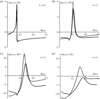
(d). The thin continuous, dashed and thick continuous lines represent the analytical, semi-analytical and numerical solutions, respectively.

6.3 Results for generalised convex boundary layer profile
Consider the generalised convex boundary layer profile defined by formulae (5.1) and (5.3) for parameters (5.2a–d
) and
 $M=1.6$
. Figure 9 shows the
 $\unicode[STIX]{x1D6FA}$
curve in the
 $\unicode[STIX]{x1D714}$
-plane for different boundary layer thicknesses obtained through various solution methods. The following observations are made.
-
(1) For thin boundary layer thickness (
$\unicode[STIX]{x1D6FF}=0.1$
or less, figure 9
a), the three solutions yield similar
$\unicode[STIX]{x1D6FA}$
curves, which are close to the curve for uniform flow. The frequency range corresponding to growing eigenmodes,
$\text{Re}\,\unicode[STIX]{x1D714}\approx 0.04{-}0.075$
, is also close to that for uniform flow, i.e. the effect of the boundary layer is not seen yet. -
(2) For increased boundary layer thickness (
$\unicode[STIX]{x1D6FF}=2$
, figure 9
b), the analytical and semi-analytical solutions are close to the numerical solution for sufficiently small
$\text{Re}\,\unicode[STIX]{x1D714}$
(namely, for
$\text{Re}\,\unicode[STIX]{x1D714}<0.14$
). For
$\text{Re}\,\unicode[STIX]{x1D714}>0.14$
, a difference between the numerical and other solutions is seen, while the semi-analytical and analytical solutions are in good agreement with each other. The frequency range of growing eigenmodes is increased to
$\text{Re}\,\unicode[STIX]{x1D714}\approx 0.09{-}0.13$
. -
(3) For
$\unicode[STIX]{x1D6FF}\geqslant 3$
, a significant difference between numerical and analytical solutions appears, because the frequencies of the growing eigenmodes increase, and the second term in the Rayleigh equation becomes essential. Figure 9(c) shows that for
$\unicode[STIX]{x1D6FF}\geqslant 3$
, the maximal growth rate
$\text{Im}\,\unicode[STIX]{x1D714}$
is lower, and the frequency range of the growing eigenmodes is higher than predicted by the analytical and semi-analytical solutions. -
(4) For
$\unicode[STIX]{x1D6FF}>3.8$
, the numerical solution shows full stabilisation of the plate by the boundary layer, whereas the analytical and semi-analytical solutions still have a range of
$\text{Re}\,\unicode[STIX]{x1D714}$
with
$\text{Im}\,\unicode[STIX]{x1D714}>0$
. An example is shown in figure 9(d) for
$\unicode[STIX]{x1D6FF}=4$
. Calculations conducted up to
$\unicode[STIX]{x1D6FF}=20$
confirm the stability of the plate obtained in the numerical solution. Other solutions predict the existence of growing eigenmodes for all
$\unicode[STIX]{x1D6FF}$
considered, though the maximum growth rate tends towards 0 as
$\unicode[STIX]{x1D6FF}$
increases.








We therefore conclude that the short-wave effect is the following. With the thickening of the boundary layer, the frequencies of growing eigenmodes increase. This yields an increasing role of the
 $k^{2}$
term in the Rayleigh equation. Calculations show that, first, due to this term, the frequencies of growing eigenmodes are higher, and the growth rates are lower than the long-wave approximation predicts. Second, starting from a certain boundary layer thickness, the plate becomes stable, whereas the long-wave approximation predicts instability for all thicknesses considered.
Note that no difference between the analytical and semi-analytical solutions is seen in this example, because, for growing eigenmodes, the condition
 $k\gg \unicode[STIX]{x1D707}^{1/3}$
is satisfied for any boundary layer thickness.
Curve
 $\unicode[STIX]{x1D6FA}$
in the
 $\unicode[STIX]{x1D714}$
-plane for the boundary layer profile (5.3) and (5.7), and boundary layer thickness
 $\unicode[STIX]{x1D6FF}=0.1$
(a),
 $\unicode[STIX]{x1D6FF}=2$
(b),
 $\unicode[STIX]{x1D6FF}=4$
(c),
 $\unicode[STIX]{x1D6FF}=6$
(d),
 $\unicode[STIX]{x1D6FF}=10$
(e) and
 $\unicode[STIX]{x1D6FF}=14$
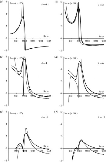
(f). The thin continuous, dashed and thick continuous lines represent the analytical, semi-analytical and numerical solutions, respectively.

6.4 Results for boundary layer profile with a generalised inflection point
Let us now consider a boundary layer profile with a generalised inflection point defined by formulae (5.3) and (5.7) for parameters (5.2a–d
) and
 $M=1.3$
.
The calculated
 $\unicode[STIX]{x1D6FA}$
curve is shown in figure 10. The following observations are made.
-
(1) For small
$\unicode[STIX]{x1D6FF}$
(figure 10
a), all solutions yield similar
$\unicode[STIX]{x1D6FA}$
curves, except for the small area
$0.016<\text{Re}\,\unicode[STIX]{x1D714}<0.02$
, where the analytical solution tends to infinity as
$\text{Re}\,c\rightarrow M-1$
for
$\unicode[STIX]{x1D6FF}=0$
. The three solutions are close to that for the uniform flow. -
(2) For higher
$\unicode[STIX]{x1D6FF}$
(figure 10
b,c), the numerical and semi-analytical solutions are still very close, predicting an increase of the frequency range for growing eigenmodes. The analytical solution looks similar, except for a narrow vicinity of
$\text{Re}\,\unicode[STIX]{x1D714}=0.02$
, where it has a dip into the stability region
$\text{Im}\,\unicode[STIX]{x1D714}<0$
. Compared to the uniform-flow results, growth rates are essentially higher, due to the increasing growth rates of downstream-travelling waves, which is demonstrated in § 5.2. -
(3) For
$\unicode[STIX]{x1D6FF}>6$
(figure 10
d), some discrepancy between the numerical and semi-analytical solutions appears, although this discrepancy is small. For small
$\text{Re}\,\unicode[STIX]{x1D714}$
, the analytical solution is essentially different from the other solutions, because for
$k\sim \unicode[STIX]{x1D707}^{1/3}$
this solution is not valid. For higher
$\text{Re}\,\unicode[STIX]{x1D714}$
(namely,
$\text{Re}\,\unicode[STIX]{x1D714}>0.023$
for
$\unicode[STIX]{x1D6FF}=6$
), the analytical and semi-analytical solutions are in good agreement with each other but differ from the numerical solution, because the condition
$k\ll 1/\unicode[STIX]{x1D6FF}$
, which is necessary for both long-wave approximations, becomes invalid. -
(4) For
$\unicode[STIX]{x1D6FF}>10$
(figure 10
e), the frequency range corresponding to growing eigenmodes continues to widen. All the solutions have two clearly marked maxima of the
$\unicode[STIX]{x1D6FA}$
curve. Starting from a certain
$\unicode[STIX]{x1D6FF}$
, both the semi-analytical and numerical solutions have a dip around
$\text{Re}\,\unicode[STIX]{x1D714}=0.017$
, where a very small piece of the
$\unicode[STIX]{x1D6FA}$
curve is located in the bottom half-plane. For the analytical solution, this dip is observed for much thinner boundary layers. The instability region is thus split into two regions separated by a very narrow frequency range of stable eigenmodes. For the numerical solution, this split occurs for
$\unicode[STIX]{x1D6FF}>12.25$
. -
(5) For
$\unicode[STIX]{x1D6FF}=14$
, results are shown in figure 10(f). It is seen that low-frequency eigenmodes become stable, and the frequency range of the growing eigenmodes is
$0.015<\text{Re}\,\unicode[STIX]{x1D714}<0.042$
, except for a narrow dip around
$\text{Re}\,\unicode[STIX]{x1D714}=0.017$
. The maximum growth rate decreases for higher
$\unicode[STIX]{x1D6FF}$
; however, the drop of
$\text{Im}\,\unicode[STIX]{x1D714}$
is much smoother than for generalised convex boundary layers; in particular, up to
$\unicode[STIX]{x1D6FF}=20$
instability is still present. For high
$\text{Re}\,\unicode[STIX]{x1D714}$
, we observe an increasing discrepancy between the numerical and other solutions due to the short-wave effect of the
$k^{2}$
term of the Rayleigh equation.








We conclude that, as well as for the generalised convex boundary layer, thickening of the boundary layer yields an increase of the frequencies of the growing eigenmodes. However, unlike for convex boundary layers, the maximum growth rate is increased for moderate thicknesses (
 $\unicode[STIX]{x1D6FF}<10$
in figure 10) compared to uniform flow. This is the result of increasing growth rates of downstream-travelling waves, as shown in § 5.2. For higher
 $\unicode[STIX]{x1D6FF}$
, the growth rates of downstream-travelling waves decrease, resulting in smaller growth rates of finite plate eigenmodes compared to those of uniform flow. However, instability is not fully suppressed up to
 $\unicode[STIX]{x1D6FF}=20$
. The short-wave effect is thus expressed in a wider unstable frequency range, while the maximum growth rate is similar to that obtained by long-wave approximations.
7 Conclusions
In this paper, we have studied short-wave panel flutter in the presence of the boundary layer. Namely, results for infinite and finite plates have been re-investigated through the full Rayleigh equation, whose
 $k^{2}$
term was neglected in the previous study (Vedeneev Reference Vedeneev2013b
). Based on two examples, one generalised convex boundary layer profile and one profile with a generalised inflection point, we confirm results obtained analytically by Vedeneev (Reference Vedeneev2013b
). Namely, for the generalised convex boundary layer, the increase of the layer thickness yields the increase of the frequencies of growing eigenmodes and the decrease of their growth rates. Calculations based on the full Rayleigh equation show that, unlike the prediction of the long-wave approximation, for sufficiently thick boundary layers, the plate is fully stabilised. For the boundary layer with a generalised inflection point, the thickening of the layer first yields the increase of the growth rates accompanied by the widening of the frequency range of growing eigenmodes. For higher thicknesses, growth rates decrease and tend towards 0 as
 $\unicode[STIX]{x1D6FF}\rightarrow \infty$
; however, they stay positive for all thicknesses considered in this study.
Although the growth rate can be increased by the boundary layer, common positive features of both types of the boundary layer profile are the damping of low-frequency modes and the increase of growing mode frequencies in the case of sufficiently thick boundary layers. It is known that structural damping (not considered in this paper) is an effective way of suppressing single-mode flutter in higher modes (Vedeneev Reference Vedeneev2013a ), while for lower modes it might be insufficient. In this case, the stabilisation mechanism of the panel can be different for lower and higher eigenmodes: lower modes can be stabilised by a boundary layer of appropriate thickness, while higher modes can be damped due to structural damping.
Based on the results of this paper, we conclude that, for accelerating supersonic flows, which usually occur along convex walls, the presence of the boundary layer has a stabilising effect, because such flows have generalised convex boundary layer profiles. On the other hand, in the flows along concave walls, a laminar boundary layer profile with a generalised inflection point may occur; in this case the boundary layer can have a destabilising effect.
When the boundary layer is turbulent, but the characteristic frequencies of the turbulence are much higher than the frequency of growing plate oscillations, the results of this study are suitable as the first approximation. As there is no evidence of turbulent boundary layers with a generalised inflection point, we conclude that turbulent boundary layers always have a stabilising effect.
The results of this paper partially explain the stabilisation of the plate by the convex boundary layer observed in the experimental and theoretical studies of Muhlstein et al. (Reference Muhlstein, Gaspers and Riddle1968), Gaspers et al. (Reference Gaspers, Muhlstein and Petroff1970), Dowell (Reference Dowell1973), Hashimoto et al. (Reference Hashimoto, Aoyama and Nakamura2009), Visbal (Reference Visbal2014) and Alder (Reference Alder2015, Reference Alder2016) but show that the effect of the boundary layer with a generalised inflection point can be essentially destabilising.
Acknowledgements
The work is supported by the grants MD-4544.2015.1 and MK-5514.2016.1.