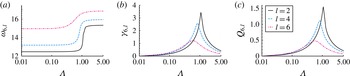
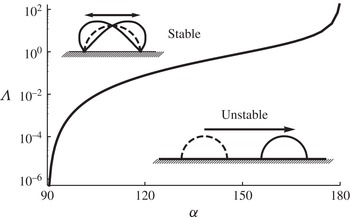
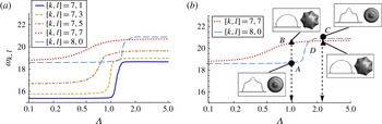
1. Introduction
Lord Rayleigh (Reference Rayleigh1879) predicted the oscillation frequencies and mode shapes for an inviscid free drop held by surface tension. The Rayleigh mode shapes are given by Legendre polynomials
 $P_{k}$
with scaled frequencies
 ${\it\lambda}_{k}$
ordered by polar wavenumber
 $k$
,
 $$\begin{eqnarray}{\it\lambda}_{k}^{2}=k(k-1)(k+2),\quad k=0,1,\dots .\end{eqnarray}$$
Here, shapes are scaled by
 $R$
, the radius of the undisturbed spherical drop, and frequencies by a capillary time scale
 $({\it\sigma}/{\it\rho}R^{3})^{-1/2}$
, where
 ${\it\sigma}$
is the surface tension and
 ${\it\rho}$
is the density of the liquid. Rayleigh’s predictions for the free drop have been verified experimentally for immiscible drops by Trinh & Wang (Reference Trinh and Wang1982) and for free drops in microgravity by Wang, Anilkumar & Lee (Reference Wang, Anilkumar and Lee1996), both using acoustic excitation.
Lamb (Reference Lamb1932) and others (e.g. Chandrasekhar Reference Chandrasekhar1961) noted that additional mode shapes also solve the Rayleigh drop equations. The Rayleigh–Lamb (RL) spectrum includes azimuthal (
 $l\neq 0$
) mode shapes
 $Y_{k}^{l}({\it\theta},{\it\psi})$
with scaled frequencies,
 ${\it\lambda}_{k,l}^{2}=k(k-1)(k+2),\ k,l=0,1,\dots$
, restricted by
 $l\leqslant k$
. Here,
 ${\it\theta}$
and
 ${\it\psi}$
are polar and azimuthal angles in spherical coordinates, respectively, and
 $Y_{k}^{l}$
is the spherical harmonic of degree
 $k$
and order
 $l$
. One should note the degeneracy of the frequencies: for every
 $k>0$
, there are distinct modes
 $l\leqslant k$
corresponding to the same
 ${\it\lambda}_{k,l}$
. The modes
 $l=0$
recover the Rayleigh modes,
 $P_{k}=Y_{k}^{0}$
, a subset of the spherical harmonics which are solutions of the Laplace equation in three dimensions (e.g. Courant & Hilbert Reference Courant and Hilbert1953).
The RL spectrum continues to see widespread use even in situations where the drop is not completely free, as for a levitated drop (Brunet & Snoeijer Reference Brunet and Snoeijer2011) or drops in contact with a solid (Noblin, Buguin & Brochard-Wyart Reference Noblin, Buguin and Brochard-Wyart2005; Dong, Chaudhury & Chaudhury Reference Dong, Chaudhury and Chaudhury2006; Chebel, Risso & Masbernat Reference Chebel, Risso and Masbernat2011) or with another liquid (Dorbolo et al. Reference Dorbolo, Terwagne, Vandewalle and Gilet2008). Modifications to (1.1), ad hoc or otherwise, are often invoked to account for the influence of substrate contact (Yoshiyasu, Matsuda & Takaki Reference Yoshiyasu, Matsuda and Takaki1996; Celestini & Kofman Reference Celestini and Kofman2006; Sharp, Farmer & Kelly Reference Sharp, Farmer and Kelly2011). Recent experiments have demonstrated the inadequacy of the RL spectrum for many sessile drop vibrations (Chang et al. Reference Chang, Bostwick, Steen and Daniel2013).
Situations where drops contact a solid support and behave nearly inviscidly are ubiquitous in traditional applications (printing, spraying, foaming, coating and condensation heat transfer), in emerging applications (digital microfluidic systems, flexible printed circuits, gradient-energy substrates) and in nature (lotus-leaf surfaces, evaporative transpiration and splashing). The need for a comprehensive theory for contacting drop and bubble oscillations has been recognized (Milne et al. Reference Milne, Defez, Cabrerizo-Vílchez and Amirfazli2014). In contrast to the free drop, which has been studied extensively since the time of Lord Rayleigh (Reference Rayleigh1879), the existing literature on the sessile drop is sparse, and particularly so for analytical-based solution methods. This occurs because supported drops possess less symmetry than free drops. Many authors have extended the pioneering work of Lord Rayleigh (Reference Rayleigh1879). Typical extensions include, but are not limited to, the effects of (i) viscosity (Lamb Reference Lamb1932; Miller & Scriven Reference Miller and Scriven1968; Prosperetti Reference Prosperetti1980), (ii) large-amplitude perturbations (Tsamopoulos & Brown Reference Tsamopoulos and Brown1983; Lundgren & Mansour Reference Lundgren and Mansour1988; Basaran & DePaoli Reference Basaran and DePaoli1994) or (iii) constrained geometries (Strani & Sabetta Reference Strani and Sabetta1984; Bostwick & Steen Reference Bostwick and Steen2009; Ilyukhina & Makov Reference Ilyukhina and Makov2009; Ramalingam & Basaran Reference Ramalingam and Basaran2010; Bostwick & Steen Reference Bostwick and Steen2013a ,Reference Bostwick and Steen b ).
Our focus is on the wetting and spreading properties of the solid substrate and their effect on fluid motion. We study the natural oscillations of an inviscid sessile drop with mobile contact lines on a planar support. Our extension embeds the RL prediction in a two-parameter family of spectra. (In this paper, ‘spectrum’ will refer to a set of eigenfrequencies and eigenmodes.) The two parameters are the volume (or equilibrium contact angle) and the mobility of the contact line. In the companion to this paper (Chang et al. Reference Chang, Bostwick, Daniel and Steen2014), the focus is experiment, and the inviscid results presented here are extended using viscous potential theory to the forced oscillation problem.
Substrate contact has three main influences on the spectrum: (i) the solid presents a barrier to liquid motion (no penetration); (ii) the solid introduces a contact line where liquid spreading is resisted (restricted contact-line mobility); (iii) the solid boundary enhances relative liquid motion, increasing the role of bulk viscosity. It should be recalled that, in the context of inviscid theory, the no-slip condition at any solid is abandoned and hence the classic viscous singularity at the moving contact line need not enter our discussion (Dussan Reference Dussan1979).
Recently, there has been a growing interest in the dynamics of sessile drops under external forcing, with an emphasis on the wetting conditions at the three-phase contact line and their motion. In drop atomization experiments, James et al. (Reference James, Vukasinovic, Smith and Glezer2003b ) and Vukasinovic, Smith & Glezer (Reference Vukasinovic, Smith and Glezer2007) observed a hierarchy of instabilities for a sessile drop (vertically) forced by a piezoelectrically driven diaphragm. Drop ejection has been studied experimentally by DePaoli et al. (Reference DePaoli, Feng, Basaran and Scott1995) and numerically using either the finite-element method (Wilkes & Basaran Reference Wilkes and Basaran2001) or a Navier–Stokes solver (James, Smith & Glezer Reference James, Smith and Glezer2003a ). In another study of mechanically vibrated sessile drops, Noblin, Buguin & Brochard-Wyart (Reference Noblin, Buguin and Brochard-Wyart2004) focused on the transition from a pinned to a free contact line and the acceleration necessary to overcome contact-angle hysteresis. Extending their previous work, Noblin et al. (Reference Noblin, Buguin and Brochard-Wyart2005) showed that at sufficiently high accelerations an azimuthal instability called the ‘triplon mode’ is generated in large fluid puddles. This instability is triggered once the contact-angle hysteresis is overcome and the contact line depins. These modes, as well as the instability observed in Vukasinovic et al. (Reference Vukasinovic, Smith and Glezer2007), exhibit subharmonic resonances, which are characteristic of Faraday waves (Faraday Reference Faraday1831; Miles & Henderson Reference Miles and Henderson1990). Chang et al. (Reference Chang, Bostwick, Steen and Daniel2013) characterized the dynamics of mechanically oscillated sessile water drops by cataloguing the first 37 mode shapes. They also observed mode mixing, or the simultaneous coexistence of multiple mode shapes within the resonating sessile drop driven by one sinusoidal signal of a single frequency.
A sessile drop subject to in-plane (horizontal) forcing exhibits an additional set of oscillatory modes that are odd or anti-symmetric about the vertical mid-plane (Sharp et al. Reference Sharp, Farmer and Kelly2011; Sharp Reference Sharp2012). Daniel et al. (Reference Daniel, Sircar, Gliem and Chaudhury2004) observed translational motion of drops on chemically treated surfaces that had overcome the hysteretic barrier or had mobile (unpinned) contact lines. A study coupling both horizontal and vertical forcing by Noblin, Kofman & Celestini (Reference Noblin, Kofman and Celestini2009) has shown that this translational motion can be directionally controlled. Brunet, Eggers & Deegan (Reference Brunet, Eggers and Deegan2009) have shown that under external forcing a sessile drop can overcome the influence of gravity and be driven up a sloped incline against gravity.
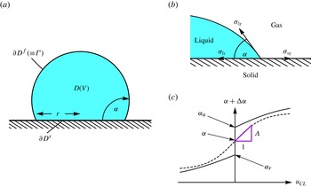
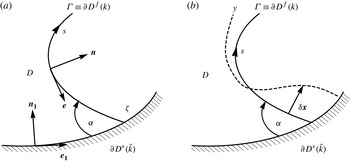
We consider a sessile drop sitting on a planar solid in a passive gas ambient, taking a spherical-cap shape which models a partially wetting drop with equilibrium contact angle
 ${\it\alpha}$
, as shown in figure 1(a). Spherical caps are scaled with the contact footprint
 $\partial D^{s}$
radius
 $r$
and volume,
 $$\begin{eqnarray}\frac{V}{r^{3}}=\frac{{\rm\pi}}{3}\frac{(2-3\cos {\it\alpha}+\cos ^{3}{\it\alpha})}{\sin ^{3}{\it\alpha}}.\end{eqnarray}$$
Accordingly, the contact angle
 ${\it\alpha}$
and drop volume
 $V$
are interchangeable parameters. We adopt
 ${\it\alpha}$
as the base-shape parameter, where
 ${\it\alpha}<{\rm\pi}/2$
is a lens-like shape and
 ${\it\alpha}>{\rm\pi}/2$
is a drop-like shape. It should be noted that the principal curvatures of the undisturbed free surface
 $\partial D^{\,f}$
are simply
 ${\it\kappa}_{1}={\it\kappa}_{2}\equiv \sin {\it\alpha}$
in our scaling. The contact angle
 ${\it\alpha}$
is related to the liquid/gas
 ${\it\sigma}_{lg}$
, liquid/solid
 ${\it\sigma}_{ls}$
and solid/gas
 ${\it\sigma}_{sg}$
interfacial tensions through the Young–Dupré equation (Young Reference Young1805; Dupré Reference Dupré1869), in the standard way,
 $$\begin{eqnarray}{\it\sigma}_{sg}-{\it\sigma}_{ls}={\it\sigma}_{lg}\cos {\it\alpha}.\end{eqnarray}$$
Figure 1(b) illustrates (1.3) as the (horizontal) balance of forces at the contact line.
Definition sketch: (a) equilibrium spherical-cap surface of base radius
 $r$
, volume
 $V$
and static contact angle
 ${\it\alpha}$
, which is defined by (b) the Young–Dupré equation (1.3) schematically illustrated as a mechanical (horizontal) force balance. The dynamic contact-line condition (c) relates the contact angle to the contact-line speed
 $u_{CL}$
with hysteresis (solid) and without (dashed). Here,
 ${\it\alpha}_{a}$
and
 ${\it\alpha}_{r}$
are the advancing and receding static contact angles (
 $u_{CL}\rightarrow 0$
), respectively. Limiting cases of the ‘continuous’ contact-line law (dashed) include the fixed contact-angle
 ${\it\Lambda}=0$
and pinned contact-line
 ${\it\Lambda}=\infty$
conditions.

Disturbances that probe the drop stability displace the contact line along the solid and, to complete the problem description, a constitutive relation for the moving contact line is needed (cf. figure 1
c). Well-accepted contact-line models include hysteresis of the non-equilibrium contact angle in order to capture the stick–slip behaviour observed in experiments, as illustrated by the solid curve in figure 1(c) (Dussan Reference Dussan1979). Contact-line speeds
 $u_{CL}>0$
correspond to liquid displacing gas;
 $u_{CL}<0$
to gas displacing liquid. However, nonlinear constitutive relations with stick–slip hysteresis are incompatible with linear analyses (Fayzrakhmanova & Straube Reference Fayzrakhmanova and Straube2009). To allow for contact-line movement in our linear analysis, we invoke the condition sketched by the dashed line in figure 1(c). This CL condition was introduced by Davis (Reference Davis1980), although it is sometimes referred to as the ‘Hocking condition’ even though Hocking (Reference Hocking1987) attributes it to Davis. This constitutive relation has been used previously in rivulet (Davis Reference Davis1980; Weiland & Davis Reference Weiland and Davis1981; Young & Davis Reference Young and Davis1987) and droplet (Lyubimov, Lyubimova & Shklyaev Reference Lyubimov, Lyubimova and Shklyaev2006; Alabuzhev & Lyubimov Reference Alabuzhev and Lyubimov2007; Fayzrakhmanova & Straube Reference Fayzrakhmanova and Straube2009; Alabuzhev & Lyubimov Reference Alabuzhev and Lyubimov2012) stability analyses. The model assumes a smooth dependence of contact-angle deviations
 ${\rm\Delta}{\it\alpha}$
on
 $u_{CL}$
, say
 ${\it\alpha}+{\rm\Delta}{\it\alpha}=f(u_{CL})$
, with
 $f(0)={\it\alpha}$
and
 $f^{\prime }(0)={\it\Lambda}$
, and linearizes to
 $$\begin{eqnarray}{\rm\Delta}{\it\alpha}={\it\Lambda}u_{CL}.\end{eqnarray}$$
The resistance to mobility,
 ${\it\Lambda}$
, or the mobility,
 ${\it\Lambda}^{-1}$
, characterizes the contact-line motion. Here,
 ${\it\Lambda}=0$
corresponds to a fully mobile contact line and
 ${\it\Lambda}=\infty$
to a pinned contact line. With this understanding, henceforth we shall refer to
 ${\it\Lambda}$
as the ‘mobility’ parameter. Davis (Reference Davis1980) showed that contact-line motion is purely dissipative for
 ${\it\Lambda}\neq 0$
. The mobility parameter may be viewed as a way to ‘deform the problem’ continuously from the mobile to the immobile contact line, and is sometimes called a homotopy or problem-deformation parameter.
We report the spectra for the sessile drop, as it depends upon
 $({\it\alpha},{\it\Lambda})$
, in terms of frequencies
 ${\it\lambda}_{k,l}$
and shapes
 $y_{k,l}(x)\cos (l{\it\psi})$
, where
 $x\equiv \cos (s)$
and
 $s$
is an arclength-like coordinate defined on the undeformed surface. Our results are conveniently framed against the RL modes. In particular, a subset of the RL modes with
 $k+l=\text{even}$
are mirror-symmetric about the equatorial plane and therefore satisfy no penetration on that mid-plane. Hence, these modes are also sessile drop solutions for the hemispherical base state (
 ${\it\alpha}=90^{\circ }$
), provided that the contact line is free (
 ${\it\Lambda}=0$
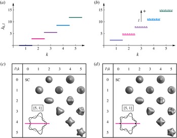
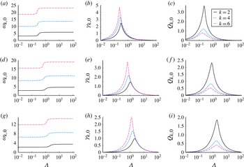
). The associated spectrum is shown in figures 2(a,c). One should note the degenerate spectrum: distinct mode shapes
 $y_{2,2}$
and
 $y_{2,0}$
have identical frequencies and, similarly, for
 $y_{3,1}$
and
 $y_{3,3}$
, and so forth. The degeneracy for the sessile drop is inherited from the free drop problem.
Symmetry breaking of modal degeneracy yields spectral splitting: the spectral lines (a)
 ${\it\lambda}_{k,l}$
for the hemispherical drop (
 ${\it\alpha}=90^{\circ }$
) exhibit a degeneracy with respect to the azimuthal wavenumber
 $l$
(c) for the (a,c) natural disturbance, which breaks for the (b,d) pinned disturbance into split spectral lines (b). Tables of mode shapes for the (c) natural and (d) pinned disturbances, as a function of polar
 $k$
and azimuthal
 $l$
wavenumbers (all with same deviation amplitude). The insets to (c) and (d) show the symmetric extension of the
 $[5,1]$
mode to the full sphere for each disturbance.

In contrast, figures 2(b,d) plot the spectrum for
 $({\it\alpha},{\it\Lambda})=(90^{\circ },\infty )$
, a preview of results in this paper. Contact-line pinning splits the frequency degeneracy; contrast figure 2(a) against figure 2(b). The splitting occurs in a way that leads to higher frequencies for higher azimuthal modes (
 $l\neq 0$
) (cf. figure 2
b). Mode shapes are superficially similar from the top view but differences can been seen near the contact line. As suggested by the
 $[5,1]$
vertical cuts with reflection about the plane of contact shown in figures 2(c,d), the (
 $90^{\circ },0$
) azimuthal modes have non-circular footprints while the (
 $90^{\circ },\infty$
) modes remain circularly pinned. It should be noted that, from the top view, the contact lines will not appear circular when overhanging shapes obstruct the contact line from sight. Our goal is to follow spectra as they deform from figures 2(a,c) to 2(b,d).
Mode
 $[1,1]$
is the only mode that is not azimuthally degenerate (cf. figure 2). Therefore, it is not subject to frequency splitting. However, it is subject to breaking another symmetry, as we shall now explain. For
 $({\it\alpha},{\it\Lambda})=(90^{\circ },0)$
, the (Rayleigh drop) problem is invariant under translation, consistent with absence of the substrate. By Noether’s theorem, there is a corresponding first integral of the motion which turns out to correspond to the mode
 $[1,1]$
, as reflected in its zero frequency. Accordingly, we shall refer to the
 $[1,1]$
mode as the ‘Noether mode’. It tends to be ignored, with few exceptions (Lyubimov, Lyubimova & Shklyaev Reference Lyubimov, Lyubimova and Shklyaev2004). For
 ${\it\Lambda}=0$
, the Noether mode corresponds to a rigid-body translation at constant velocity (Galilean translation). For
 ${\it\Lambda}>0$
, the substrate begins to exert an influence and the symmetry of translational invariance is broken. The laboratory frame comes into play. For
 ${\it\Lambda}>0$
, the Noether mode becomes time-dependent and, for
 ${\it\Lambda}=\infty$
, its frequency approaches
 ${\it\lambda}_{1,1}\sim 2.5$
, as shown in figure 2(b). The situation is quite different for the unpinned Noether mode (
 ${\it\Lambda}\neq \infty$
), which can have imaginary frequencies and hence can exhibit instability.
A few special cases of natural oscillations for a sessile drop have been previously studied analytically. All studies have been restricted to hemispherical base states. Lyubimov et al. (Reference Lyubimov, Lyubimova and Shklyaev2004) introduced a homotopy parameter, like
 ${\it\Lambda}$
, and reported frequencies for the first eight broken modes (up to
 $k=4$
in figure 2
b), along with the attenuation introduced by the contact-line motion. The Noether mode is referred to as a ‘bending’ oscillation. Lyubimov et al. (Reference Lyubimov, Lyubimova and Shklyaev2006) reported natural frequencies of the first three axisymmetric modes, along with attenuation. Fayzrakhmanova & Straube (Reference Fayzrakhmanova and Straube2009) showed how to maintain Hocking stick–slip hysteresis while proceeding analytically; their analysis is necessarily nonlinear. The restriction to hemispherical base states is related to the need to solve Laplace’s equations analytically. The key innovation that allows non-hemispherical base states here is solution of the Laplace equation in hybrid coordinates. This approach could be extended to bridges, rivulets and other heretofore intractable base-state shapes.
We begin this paper with the hydrodynamic equations associated with small disturbances to the spherical-cap interface. We consider disturbances whose three-phase contact line is (i) pinned, (ii) moves with fixed contact angle and (iii) moves with a contact angle that is a smooth function of the contact-line speed. The governing equations are reduced by a normal-mode expansion to a functional eigenvalue problem on linear operators. We use inverse operators to construct a solution for disturbances (i) and (ii) and report frequencies and modal structures distinguished by a polar
 $k$
and azimuthal
 $l$
wavenumber. We illustrate the spectral dependence on
 ${\it\alpha}$
and compare disturbances (i) and (ii). For the dynamic contact-line condition (iii), we use an alternative solution method to derive an operator equation in the form of a damped-harmonic oscillator with dissipation controlled by
 ${\it\Lambda}$
. The relationship between the wetting properties of the substrate, the modal structure and dissipation is illustrated. Lastly, some concluding remarks are offered.
2. Mathematical formulation
The sessile drop is a surface of constant mean curvature
 $H$
and equivalently a static equilibrium configuration according to the Young–Laplace equation,
 $$\begin{eqnarray}\frac{p}{{\it\sigma}}={\it\kappa}_{1}+{\it\kappa}_{2}\equiv 2H,\end{eqnarray}$$
which relates the principal curvatures,
 ${\it\kappa}_{1}$
and
 ${\it\kappa}_{2}$
, to the pressure
 $p$
there. The equilibrium surface
 ${\it\Gamma}$
is defined parametrically as
 $$\begin{eqnarray}X(s,{\it\varphi};{\it\alpha})=\frac{\sin (s)}{\sin ({\it\alpha})}\cos ({\it\varphi}),\quad Y(s,{\it\varphi};{\it\alpha})=\frac{\sin (s)}{\sin ({\it\alpha})}\sin ({\it\varphi}),\quad Z(s;{\it\alpha})=\frac{\cos (s)-\cos ({\it\alpha})}{\sin ({\it\alpha})},\end{eqnarray}$$
using arclength-like
 $s\in [0,{\it\alpha}]$
and azimuthal angle
 ${\it\varphi}\in [0,2{\rm\pi}]$
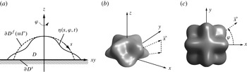
as generalized surface coordinates. The interface is given a small perturbation
 ${\it\eta}(s,{\it\varphi},t)$
(cf. figure 3). No domain perturbation is needed for small deformations, thus the droplet domain
 $$\begin{eqnarray}D\equiv \{(x,y,z)\mid 0\leqslant x\leqslant X(s,{\it\varphi};{\it\alpha}),\,0\leqslant y\leqslant Y(s,{\it\varphi};{\it\alpha}),\,0\leqslant z\leqslant Z(s;{\it\alpha})\}\end{eqnarray}$$
is bounded by a free surface
 $\partial D^{f}(\equiv {\it\Gamma})$
of constant surface tension
 ${\it\sigma}$
(no thermocapillary effects), and a planar surface-of-support
 $\partial D^{s}$
,
 $$\begin{eqnarray}\partial D^{f}\equiv \{\left(x,y,z\right)\mid x=X(s,{\it\varphi};{\it\alpha}),y=Y(s,{\it\varphi};{\it\alpha}),\,z=Z(s;{\it\alpha})\},\,\quad \partial D^{s}\equiv \{\left(x,y,z\right)\mid z=0\}.\end{eqnarray}$$
The droplet is immersed in a passive gas and the effect of gravity is neglected.
Definition sketch with the unperturbed
 ${\it\Gamma}$
(dashed) and perturbed interface
 ${\it\eta}$
(solid) in (a) polar cross-section and three-dimensional (b) perspective and (c) top views.

2.1. Hydrodynamic field equations
The fluid is incompressible and the flow is assumed to be irrotational. Therefore, the velocity field may be described as
 $\boldsymbol{v}=-\boldsymbol{{\rm\nabla}}{\it\Psi}$
, where the velocity potential
 ${\it\Psi}$
satisfies Laplace’s equation
 $$\begin{eqnarray}{\rm\nabla}^{2}{\it\Psi}=0\quad [D]\end{eqnarray}$$
on the drop domain. Additionally, the velocity potential satisfies the no-penetration condition
 $$\begin{eqnarray}\boldsymbol{{\rm\nabla}}{\it\Psi}\boldsymbol{\cdot }\hat{\boldsymbol{z}}=0\quad [\partial D^{s}]\end{eqnarray}$$
on the surface-of-support and a (linearized) kinematic condition
 $$\begin{eqnarray}\frac{\partial {\it\Psi}}{\partial n}=-\frac{\partial {\it\eta}}{\partial t}\quad [\partial D^{f}]\end{eqnarray}$$
on the free surface, which relates the normal velocity to the perturbation amplitude there. In the limit of small interface deflection and in accordance with potential flow theory, the pressure field is expressed by the linearized Bernoulli equation
 $$\begin{eqnarray}p={\it\varrho}\frac{\partial {\it\Psi}}{\partial t}\quad [D],\end{eqnarray}$$
where
 ${\it\varrho}$
is the fluid density. Finally, disturbances to the equilibrium surface
 ${\it\Gamma}$
generate pressure gradients, and thereby flows, according to the Young–Laplace equation
 $$\begin{eqnarray}p/{\it\sigma}=-{\it\Delta}_{{\it\Gamma}}{\it\eta}-\left({\it\kappa}_{1}^{2}+{\it\kappa}_{2}^{2}\right){\it\eta}\quad [\partial D^{f}],\end{eqnarray}$$
where the Laplace–Beltrami operator
 ${\it\Delta}_{{\it\Gamma}}$
, which depends on
 ${\it\Gamma}$
, will be defined below.
The hydrodynamic field equations (2.5)–(2.9) govern the motion of an inviscid fluid, whose spherical-cap interface is given a small disturbance. The field equations must be augmented with a boundary condition on the three-phase contact line to yield a well-posed system of partial differential equations, a condition that we discuss later.
2.2. Laplace–Beltrami operator
The Laplace–Beltrami operator
 ${\it\Delta}_{{\it\Gamma}}$
, introduced in (2.9), depends on equilibrium-surface curvatures and operates on functions
 ${\it\eta}$
,
 $$\begin{eqnarray}{\it\Delta}_{{\it\Gamma}}{\it\eta}\equiv \frac{1}{\sqrt{g}}\frac{\partial }{\partial u^{{\it\mu}}}\left(\sqrt{g}g^{{\it\mu}{\it\nu}}\frac{\partial {\it\eta}}{\partial u^{{\it\nu}}}\right),\end{eqnarray}$$
with the surface metric given by
 $$\begin{eqnarray}g_{{\it\mu}{\it\nu}}\equiv \boldsymbol{x},_{{\it\mu}}\boldsymbol{x},_{{\it\nu}}=\left(\begin{array}{@{}cc@{}}\text{csc}^{2}({\it\alpha}) & 0\\ 0 & \left(\text{csc}({\it\alpha})\sin (s)\right)^{2}\end{array}\right),\quad g=\left(\sin (s)\text{csc}^{2}({\it\alpha})\right)^{2},\end{eqnarray}$$
and
 ${\it\mu},{\it\nu}=1,2$
, using notation standard to differential geometry (e.g. Kreyszig Reference Kreyszig1991).
2.3. Normal-mode reduction
Normal modes, parameterized by frequency
 ${\it\Omega}$
and azimuthal wavenumber
 $l$
,
 $$\begin{eqnarray}{\it\eta}(s,{\it\varphi},t)=y(s)\text{e}^{\text{i}{\it\Omega}t}\text{e}^{\text{i}l{\it\varphi}},\quad {\it\Psi}(\boldsymbol{x},t)={\it\phi}({\it\rho},{\it\theta})\text{e}^{\text{i}{\it\Omega}t}\text{e}^{\text{i}l{\it\varphi}},\end{eqnarray}$$
are applied to the field equations (2.5)–(2.9) to yield
 $$\begin{eqnarray}\displaystyle & \displaystyle \frac{\partial }{\partial {\it\rho}}\left({\it\rho}^{2}\frac{\partial {\it\phi}}{\partial {\it\rho}}\right)+\frac{1}{\sin {\it\theta}}\frac{\partial }{\partial {\it\theta}}\left(\sin {\it\theta}\frac{\partial {\it\phi}}{\partial {\it\theta}}\right)-\frac{l^{2}}{\sin ^{2}{\it\theta}}{\it\phi}=0\quad [D], & \displaystyle\end{eqnarray}$$
 $$\begin{eqnarray}\displaystyle & \displaystyle \frac{\partial {\it\phi}}{\partial n}=0\quad [\partial D^{s}], & \displaystyle\end{eqnarray}$$
 $$\begin{eqnarray}\displaystyle & \displaystyle \frac{\partial {\it\phi}}{\partial n}=-\text{i}{\it\lambda}y\quad [\partial D^{f}], & \displaystyle\end{eqnarray}$$
 $$\begin{eqnarray}\displaystyle & \displaystyle y^{\prime \prime }+\cot (s)y^{\prime }+\left(2-\frac{l^{2}}{\sin ^{2}(s)}\right)y=-\text{i}{\it\lambda}\csc ^{2}({\it\alpha}){\it\phi}\quad [\partial D^{f}], & \displaystyle\end{eqnarray}$$
 $$\begin{eqnarray}\displaystyle & \displaystyle \int _{{\it\Gamma}}\frac{\partial {\it\phi}}{\partial n}\text{d}{\it\Gamma}=0, & \displaystyle\end{eqnarray}$$
 $$\begin{eqnarray}\displaystyle & \displaystyle {\it\lambda}^{2}\equiv \frac{{\it\varrho}{\it\Omega}^{2}r^{3}}{{\it\sigma}}. & \displaystyle\end{eqnarray}$$
 ${\it\rho},{\it\theta}$
), (2.13b
) is the no-penetration condition on the support surface, (2.13c
) is the kinematic condition and (2.13e
) is the integral form of the incompressibility condition or a volume conservation constraint. The dynamic pressure balance across the free surface is represented by (2.13d
) with differentiation with respect to the arclength coordinate
 $\text{}^{\prime }=\text{d}/\text{d}s$
. Equations (2.13) are an eigenvalue problem in the scaled frequency
 ${\it\lambda}$
, defined in (2.13f
).
3. Reduction to operator equation
The dynamic pressure balance (2.13d ) can be rewritten using (2.13c ),
 $$\begin{eqnarray}\left(\frac{\partial {\it\phi}}{\partial n}\right)^{\prime \prime }+\cot (s)\left(\frac{\partial {\it\phi}}{\partial n}\right)^{\prime }+\left(2-\frac{l^{2}}{\sin ^{2}(s)}\right)\left(\frac{\partial {\it\phi}}{\partial n}\right)=-\frac{{\it\lambda}^{2}}{\sin ^{2}({\it\alpha})}{\it\phi}\quad [\partial D^{f}].\end{eqnarray}$$
3.1. Operator formalism
This integrodifferential equation governs the motion of the interface and may be formulated as a operator equation by two alternative representations.
3.1.1. Direct problem: unknown interface deflection
The first formulation uses the interface deflection
 $\partial {\it\phi}/\partial n$
as the unknown function,
 $$\begin{eqnarray}K\left[\frac{\partial {\it\phi}}{\partial n};l\right]=-\hat{{\it\lambda}}^{2}M\left[\frac{\partial {\it\phi}}{\partial n}\right],\quad \hat{{\it\lambda}}^{2}\equiv \frac{{\it\lambda}^{2}}{\sin ^{2}({\it\alpha})},\end{eqnarray}$$
which we refer to as the direct problem. Here,
 $M$
is an integral operator representative of the fluid inertia and
 $K$
is a differential operator related to the curvature,
 $$\begin{eqnarray}\displaystyle & \displaystyle M\left[\frac{\partial {\it\phi}}{\partial n}\right]\equiv {\it\phi}, & \displaystyle\end{eqnarray}$$
 $$\begin{eqnarray}\displaystyle & \displaystyle K\left[\frac{\partial {\it\phi}}{\partial n};l\right]\equiv \left(\frac{\partial {\it\phi}}{\partial n}\right)^{\prime \prime }+\cot (s)\left(\frac{\partial {\it\phi}}{\partial n}\right)^{\prime }+\left(2-\frac{l^{2}}{\sin ^{2}(s)}\right)\left(\frac{\partial {\it\phi}}{\partial n}\right). & \displaystyle\end{eqnarray}$$
 $$\begin{eqnarray}{\rm\nabla}^{2}{\it\phi}=0\quad [D],\quad \frac{\partial {\it\phi}}{\partial n}=f_{k}\quad [\partial D^{f}].\end{eqnarray}$$
More specifically, given a surface deformation
 $f_{k}$
, one needs to compute the corresponding velocity potential
 ${\it\phi}_{k}$
, in accordance with the inertia operator (3.3a
). In general, for all but the simplest of geometries, solution of this Neumann-type boundary-value problem requires a computationally intensive approach.
3.1.2. Inverse problem: unknown velocity potential
Alternatively, one may use the velocity potential
 ${\it\phi}$
as the unknown function,
 $$\begin{eqnarray}M^{-1}\left[{\it\phi}\right]=-\hat{{\it\lambda}}^{2}K^{-1}\left[{\it\phi};l\right],\end{eqnarray}$$
which follows directly from (3.2) and is referred to as the inverse problem. Here, the integrodifferential nature of the governing equation persists, with
 $$\begin{eqnarray}M^{-1}\left[{\it\phi}\right]\equiv \frac{\partial {\it\phi}}{\partial n}\end{eqnarray}$$
the differential operator and
 $K^{-1}$
an integral operator, inversely related to the curvature operator
 $K$
defined in (3.3b
). As with the direct problem, the primary difficulties associated with the inverse problem are related to the integral operator. Specifically, construction of the inverse operator
 $K^{-1}$
depends on the parametrization of the equilibrium surface and may or may not be analytically tractable.
3.1.3. Direct versus inverse problem
The two representations defined here are completely equivalent, but each has its respective solution difficulties. In the direct problem, one has to construct a sufficiently general solution to Laplace’s equation with Neumann boundary conditions. In most cases, this is analytically intractable. Likewise, with the inverse operator formalism, one must construct the Green’s function to the differential curvature operator. While the inverse problem is seen to be more tractable in general, the direct problem has an attractive variational structure that will be exploited in a subsequent section.
3.2. Contact-line conditions
To compute the spectrum of the eigenvalue problem (2.13), one needs to specify the type of disturbance via a boundary condition on the three-phase contact line. We decompose the solutions into two distinct classes, kinematic and dynamic. Kinematic disturbances depend solely upon the interface deflection, whereas dynamic disturbances are related to dynamic field quantities, such as the contact-line speed. For all contact-line boundary conditions, to ensure that the boundary-value problem is well-posed mathematically, we require
 $$\begin{eqnarray}\left.\frac{\partial {\it\phi}}{\partial n}\right|_{s=0}-\text{bounded},\end{eqnarray}$$
a necessary condition which guarantees that the interface disturbance is physical.
3.2.1. Natural (fixed contact angle)
The first type of kinematic disturbance preserves the static contact angle
 ${\it\alpha}$
,
 $$\begin{eqnarray}\left.\frac{\partial }{\partial s}\left(\frac{\partial {\it\phi}}{\partial n}\right)+\cos ({\it\alpha})\frac{\partial {\it\phi}}{\partial n}=0\right|_{s={\it\alpha}},\end{eqnarray}$$
and corresponds to the ‘natural’ boundary condition related to the linearized Young–Dupré equation. A derivation of (3.8) is given in appendix A.
3.2.2. Pinned (fixed contact line)
The second type of kinematic disturbance has an immobile contact line,
 $$\begin{eqnarray}\left.\frac{\partial {\it\phi}}{\partial n}\right|_{s={\it\alpha}}=0,\end{eqnarray}$$
and is referred to as the ‘pinned’ contact-line condition. Courant & Hilbert (Reference Courant and Hilbert1953, chap. 6, p. 410) show that the pinned contact-line disturbance is the most restrictive for the general boundary-value problem.
3.2.3. Dynamic contact line
The dynamic contact-line condition follows by assuming that the contact angle depends smoothly on the contact-line speed through the function
 $f$
(cf. figure 1
c). Assuming normal modes for contact-angle deviation,
 ${\rm\Delta}{\it\alpha}={\it\epsilon}\hat{{\it\alpha}}\text{e}^{\text{i}{\it\Omega}t}\text{e}^{\text{i}l{\it\varphi}}$
, setting
 $\partial {\it\eta}/\partial t=u_{CL}$
, and applying (2.13c
) to (1.4) allows one to obtain the reduced variation in contact angle,
 $$\begin{eqnarray}{\it\alpha}+{\it\epsilon}\hat{{\it\alpha}}=f\left(0+{\it\epsilon}\,\left(\frac{\partial {\it\phi}}{\partial n}\right)\right);\quad \hat{{\it\alpha}}={\it\Lambda}\,\left(\frac{\partial {\it\phi}}{\partial n}\right);\ {\it\Lambda}\equiv f^{\prime }(0).\end{eqnarray}$$
Applying (3.10) to the linearized Young–Dupré equation (A 10) gives
 $$\begin{eqnarray}\frac{\partial }{\partial s}\left(\frac{\partial {\it\phi}}{\partial n}\right)+\cos ({\it\alpha})\left(\frac{\partial {\it\phi}}{\partial n}\right)=\left.\text{i}{\it\lambda}{\it\Lambda}\left(\frac{\partial {\it\phi}}{\partial n}\right)\right|_{s={\it\alpha}}.\end{eqnarray}$$
Here,
 $1/{\it\Lambda}$
is a measure of the mobility of the contact line, which smoothly ‘deforms’ the boundary from a natural (fully mobile) to a pinned (immobile) condition. This is sometimes called a ‘homotopy’ parameter. In the limits
 ${\it\Lambda}\rightarrow 0,\infty$
, (3.11) reduces to (3.8), (3.9), respectively.
4. Method for kinematic disturbances: natural and pinned contact lines
As stated earlier, the spectrum of the operator (3.1) may be computed from either the direct or the inverse problem. For the kinematic disturbances, we compute the spectrum from the inverse problem (3.5).
4.1. Inverse operator
The kinematic disturbances, natural and pinned, are structurally similar, and we derive the respective inverse operators simultaneously. To use the inverse operator formalism, one must construct the integral operator,
 $$\begin{eqnarray}K^{-1}\left[{\it\phi}\right](x)=\int _{b}^{1}G\left(x,y;l\right){\it\phi}(y)\text{d}y,\end{eqnarray}$$
or fundamental solution (Green’s function) of the curvature operator (3.3b ),
 $$\begin{eqnarray}G\left(x,y;l\right)=\left\{\begin{array}{@{}ll@{}}\displaystyle {\it\xi}(l)y_{1}(y;l)\left[\frac{{\it\tau}_{2}(l)}{{\it\tau}_{1}(l)}y_{1}(x;l)-y_{2}(x;l)\right],\quad & b<x<y<1,\\ \displaystyle {\it\xi}(l)y_{1}(x;l)\left[\frac{{\it\tau}_{2}(l)}{{\it\tau}_{1}(l)}y_{1}(y;l)-y_{2}(y;l)\right],\quad & b<y<x<1,\end{array}\right.\end{eqnarray}$$
where
 $$\begin{eqnarray}\displaystyle x\equiv \cos (s),\quad b\equiv \cos ({\it\alpha}). & & \displaystyle\end{eqnarray}$$
The Green’s function is parameterized by the azimuthal wavenumber
 $l$
and the transformed contact angle
 $b$
. The functions
 $y_{1}$
and
 $y_{2}$
belong to the kernel of the curvature operator
 $K$
and are given by
 $$\begin{eqnarray}\displaystyle \left.\begin{array}{@{}l@{}}y_{1}(x;0)=P_{1}(x),\quad y_{2}(x;0)=Q_{1}(x),\quad y_{1}(x;1)=P_{1}^{(1)}(x),\quad y_{2}(x;1)=Q_{1}^{(1)}(x),\\ \displaystyle y_{1}(x;l\geqslant 2)=\left(x+l\right)\left(\frac{1-x}{1+x}\right)^{l/2},\quad y_{2}(x;l\geqslant 2)=\frac{\left(x+l\right)}{2l\left(l^{2}-1\right)}\left(\frac{1+x}{1-x}\right)^{l/2},\end{array}\right\} & & \displaystyle \nonumber\\ \displaystyle & & \displaystyle\end{eqnarray}$$
where
 $P_{1},Q_{1}$
and
 $P_{1}^{(1)},Q_{1}^{(1)}$
are the order 0 and 1 Legendre functions of index 1, respectively (MacRobert Reference MacRobert1967). Similarly, the scale factor is given by
 $$\begin{eqnarray}{\it\xi}(l)\equiv \left\{\begin{array}{@{}ll@{}}{\textstyle \frac{1}{2}},\quad & l=1,\\ 1,\quad & l\neq 1,\end{array}\right.\end{eqnarray}$$
while the parameters
 ${\it\tau}_{1}$
and
 ${\it\tau}_{2}$
are related to the contact-line boundary conditions
 $$\begin{eqnarray}{\it\tau}_{1}^{(n)}=y_{1}^{\prime }(b;l)+\frac{b}{\sqrt{1-b^{2}}}y_{1}(b;l),\quad {\it\tau}_{2}^{(n)}=y_{2}^{\prime }(b;l)+\frac{b}{\sqrt{1-b^{2}}}y_{2}(b;l)\end{eqnarray}$$
for the natural disturbance (superscript
 $n$
) and
 $$\begin{eqnarray}{\it\tau}_{1}^{(p)}=y_{1}(b;l),\quad {\it\tau}_{2}^{(p)}=y_{2}(b;l)\end{eqnarray}$$
for the pinned contact-line disturbance (superscript
 $p$
), respectively.
4.1.1. Axisymmetric operator
 $(l=0)$

To satisfy the conservation of volume constraint (2.13e
), we recall that the velocity potential
 ${\it\phi}$
is defined up to an arbitrary constant
 $C$
, which allows one to write (3.5) as
 $$\begin{eqnarray}\frac{\partial {\it\phi}}{\partial n}(x)=-\hat{{\it\lambda}}^{2}\left[C\int _{b}^{1}G(x,y;0)\text{d}y+\int _{b}^{1}G(x,y;0){\it\phi}(y)\text{d}y\right].\end{eqnarray}$$
Integrating (4.8) along the equilibrium surface and enforcing (2.13e ) determines
 $$\begin{eqnarray}C=-\frac{\displaystyle \int _{b}^{1}\int _{b}^{1}G(x,y;0){\it\phi}(y)\text{d}y\text{d}x}{\displaystyle \int _{b}^{1}\int _{b}^{1}G(x,y;0)\text{d}y\text{d}x}.\end{eqnarray}$$
Finally, applying (4.9) to (4.8) results in the following functional eigenvalue equation:
 $$\begin{eqnarray}\frac{\partial {\it\phi}}{\partial n}(x)=\hat{{\it\lambda}}^{2}\left[\frac{\displaystyle \int _{b}^{1}\int _{b}^{1}G(x,y;0){\it\phi}(y)\text{d}y\text{d}x}{\displaystyle \int _{b}^{1}\int _{b}^{1}G(x,y;0)\text{d}y\text{d}x}\int _{b}^{1}G(x,y;0)\text{d}y-\int _{b}^{1}G(x,y;0){\it\phi}(y)\text{d}y\right],\end{eqnarray}$$
with volume conserved for all functions
 ${\it\phi}$
.
4.1.2. Azimuthal operator
$(l\neq 0)$

The volume conservation constraint (2.13e
) is naturally satisfied for disturbances with azimuthal wavenumber
 $l\geqslant 1$
. Thus, the corresponding operator equation is given by
 $$\begin{eqnarray}\frac{\partial {\it\phi}}{\partial n}(x)=-\hat{{\it\lambda}}^{2}\left[\int _{b}^{1}G(x,y;l){\it\phi}(y)\text{d}y\right].\end{eqnarray}$$
4.2. Computational evaluation: Rayleigh–Ritz
The eigenvalue spectrum of (4.10) and (4.11) can be evaluated in any number of ways. We reduce the operator equations to a truncated set of linear algebraic equations using the Rayleigh–Ritz variational procedure. The stationary values of the functional
 $$\begin{eqnarray}\hat{{\it\lambda}}^{2}=\frac{\left(-M^{-1}\left[{\it\phi}\right],{\it\phi}\right)}{\left(K^{-1}\left[{\it\phi}\right],{\it\phi}\right)},\quad {\it\phi}\in S,\end{eqnarray}$$
are the characteristic oscillation frequencies, where
 $S$
is a predetermined function space. We choose this function space to satisfy Laplace’s equation (2.13a
) and the no-penetration condition (2.13b
). In this case, the minimizers of (4.10) and (4.11) are also solutions to the eigenvalue problem (2.13). We sketch the method here, while a more thorough illustration can be found in Segel (Reference Segel1987).
The necessary input for the Rayleigh–Ritz procedure is a solution series
 $$\begin{eqnarray}{\it\phi}=\mathop{\sum }\limits_{j=1}^{N}a_{j}{\it\phi}_{j}^{(l)},\end{eqnarray}$$
constructed from basis functions
 ${\it\phi}_{j}^{(l)}$
. These functions are applied to (4.10) and (4.11) and inner products are taken to generate a set of linear algebraic equations
 $$\begin{eqnarray}\mathop{\sum }\limits_{j=1}^{N}\left(m_{ij}^{(l)}-\hat{{\it\lambda}}^{2}{\it\kappa}_{ij}^{(l)}\right)a_{j}=0_{i},\end{eqnarray}$$
with
 $$\begin{eqnarray}m_{ij}^{(l)}\equiv \int _{b}^{1}\left(\frac{\partial {\it\phi}_{i}^{(l)}}{\partial n}\right){\it\phi}_{j}^{(l)}\text{d}x,\quad {\it\kappa}_{ij}^{(l)}\equiv \left(\frac{G_{i0}G_{0j}}{G_{00}}{\it\delta}_{l,0}-G_{ij}\right),\end{eqnarray}$$
where
 ${\it\delta}_{l,0}$
is the Kronecker delta,
 ${\it\delta}_{0,0}=1$
and
 ${\it\delta}_{l,0}=0$
if
 $l\neq 0$
, and
 $$\begin{eqnarray}\displaystyle \frac{G_{ij}}{{\it\xi}(l)} & \equiv & \displaystyle \left[\int _{b}^{1}y_{1}(x;l){\it\phi}_{i}^{(l)}(x)\,\text{d}x\right]\left[\int _{b}^{1}\left(\frac{{\it\tau}_{2}}{{\it\tau}_{1}}y_{1}(x;l)-y_{2}(x;l)\right){\it\phi}_{j}^{(l)}(x)\,\text{d}x\right]\nonumber\\ \displaystyle & & \displaystyle +\,\int _{b}^{1}y_{1}(x;l){\it\phi}_{i}^{(l)}(x)\int _{x}^{1}y_{2}(y;l){\it\phi}_{j}^{(l)}(y)\text{d}y\text{d}x\nonumber\\ \displaystyle & & \displaystyle -\,\int _{b}^{1}y_{2}(x;l){\it\phi}_{i}^{(l)}(x)\int _{x}^{1}y_{1}(y;l){\it\phi}_{j}^{(l)}(y)\text{d}y\text{d}x.\end{eqnarray}$$
Allowable solutions of the operator equation (4.10), (4.11) must satisfy the hydrodynamic field equations (2.13). We recall that volume conservation (2.13e
) has been satisfied by proper selection of the constant
 $C$
and the contact-line conditions are incorporated into the Green’s function (4.2), but the no-penetration condition (2.13b
) has yet to be satisfied. This can be accomplished through proper selection of the basis functions,
 $$\begin{eqnarray}{\it\phi}_{j}^{(l)}({\it\rho},{\it\theta})={\it\rho}^{j}P_{j}^{(l)}\left(\cos {\it\theta}\right),\end{eqnarray}$$
written here in spherical coordinates,
 ${\it\rho}$
and
 ${\it\theta}$
, and chosen to be harmonic, as required by (2.13a
). Here,
 $P_{j}^{(l)}$
is the Legendre function of degree
 $j$
and order
 $l$
. The following restriction on the polar
 $j$
and azimuthal
 $l$
wavenumbers is sufficient to ensure that the no-penetration condition (2.13b
) is satisfied:
 $l+j=\text{even}$
. Additionally, a consistency condition requires
 $l\leqslant j$
.
The normal derivatives of the basis functions (4.17), evaluated on the equilibrium surface, are expressed as
 $$\begin{eqnarray}\displaystyle \frac{\partial {\it\phi}_{j}^{(l)}}{\partial n} & \equiv & \displaystyle \boldsymbol{{\rm\nabla}}{\it\phi}_{j}^{(l)}\boldsymbol{\cdot }\boldsymbol{n}=jP_{j}^{(l)}\left(\cos {\it\theta}\right)\left(-\text{sin}\,s\sin {\it\theta}+\cos s\cos {\it\theta}\right)\left({\it\rho}\right)^{j-1}\nonumber\\ \displaystyle & & \displaystyle +\,\sin {\it\theta}P_{j}^{\prime (l)}\left(\cos {\it\theta}\right)\left(\sin s\cos {\it\theta}+\cos s\sin {\it\theta}\right)\left({\it\rho}\right)^{j-1},\end{eqnarray}$$
using mixed coordinates for efficiency in presentation. To compute the matrix elements (4.15a,b ), the basis functions (4.17) and their normal derivatives (4.18) are evaluated on the equilibrium surface using the following coordinate transformation:
 $$\begin{eqnarray}{\it\rho}\equiv \sqrt{X^{2}+Y^{2}+Z^{2}},\quad \cos {\it\theta}\equiv \frac{Z}{\sqrt{X^{2}+Y^{2}+Z^{2}}},\quad \sin {\it\theta}\equiv \sqrt{\frac{X^{2}+Y^{2}}{X^{2}+Y^{2}+Z^{2}}},\end{eqnarray}$$
which relates spherical coordinates, whose origin is centred on the surface-of-support, to the arclength coordinate. Here,
 $X=X(s),\ Y=Y(s),\ Z=Z(s)$
have been defined in (2.2). Finally, the basis functions (4.17) are applied to (4.15a,b
) to generate a set of algebraic equations (4.14), from which the characteristic oscillation frequencies are computed.
The eigenvalues
 ${\it\lambda}_{k,l}$
of (4.14) have been computed using a resolution of
 $N=10$
basis functions in the solution series (4.13) for both natural and pinned disturbances, as they depend upon the contact angle
 ${\it\alpha}$
and azimuthal wavenumber
 $l$
. The eigenfunction
 ${\it\phi}_{k,l}$
associated with the eigenfrequency
 ${\it\lambda}_{k,l}$
and corresponding eigenvector
 $a_{j}^{(k,l)}$
is given by
 $$\begin{eqnarray}{\it\phi}_{k,l}(x)=\mathop{\sum }\limits_{j=1}^{N}a_{j}^{(k,l)}{\it\phi}_{j}^{(l)}(x).\end{eqnarray}$$
Here, eigenfrequencies/eigenvectors are distinguished by polar
 $k$
and azimuthal
 $l$
wavenumbers. Similarly, the corresponding interface deformation
 $y_{k,l}$
is expressed as
 $$\begin{eqnarray}y_{k,l}(x)=\mathop{\sum }\limits_{j=1}^{N}a_{j}^{(k,l)}\left(\frac{\partial {\it\phi}_{j}^{(l)}}{\partial n}\right)(x).\end{eqnarray}$$
5. Validation of computations
Prior computations for special limiting cases provide validation of our model. Our solutions naturally reduce to the RL spectrum in the limit of
 $({\it\alpha},{\it\Lambda})\rightarrow (90^{\circ },0)$
. The axisymmetric pinned
 $[2,0]$
mode has been simulated by the finite-element method for a range of
 ${\it\alpha}$
by Basaran & DePaoli (Reference Basaran and DePaoli1994); the comparison with our results is shown in figure 6(b) of § 7.1. Comparison with observation provides further corroboration. Frequencies of water droplets excited by a puff of air have been reported by Sharp et al. (Reference Sharp, Farmer and Kelly2011) for a range of
 ${\it\alpha}$
. The reported mode shape has the character of the
 $[1,1]$
rocking mode; comparison against our prediction is shown in figure 7(b) of § 7.2. Further comparison against experiment is the subject of Chang et al. (Reference Chang, Bostwick, Steen and Daniel2013), where reasonable agreement is reported. Chang et al. (Reference Chang, Bostwick, Daniel and Steen2014) report further tests of theory against experiment.
6. Mode-shape terminology and overview of results
Figures 2(c,d) suggest a spherical harmonic classification by wavenumber pair
 $[k,l]$
inherited from the RL modes, even though, for
 $({\it\alpha},{\it\Lambda})\neq (90^{\circ },0)$
, the spherical harmonic shapes are not solutions to the governing equations (3.2). According to the spherical harmonic terminology, mode shapes are categorized as zonal (
 $l=0$
), sectoral (
 $k=l$
) and tesseral (
 $l\neq 0,k\neq l$
) (e.g. MacRobert Reference MacRobert1967). This classification scheme is equivalent to identifying nodes (zeros) of the interface shape
 $y_{k,l}$
, the geometric curve formed by the intersection of the disturbed shape with the undisturbed shape. Nodes may be composed of circles of both latitude and longitude. One can determine the number of nodal lines by counting the number of zeros of
 $y_{k,l}$
in the latitudinal and longitudinal directions, independently. Given a natural mode with wavenumber pair
 $[k,l]$
, there are precisely
 $l$
longitudinal and
 $(k-l)/2$
latitudinal intersections (zeros) of the undisturbed shape. Zonal modes (
 $l=0$
) are axisymmetric and intersect the undisturbed shape only along latitudinal lines. In contrast, sectoral modes (
 $k=l$
) have only longitudinal intersections. Mode shapes with both types of nodes are referred to as tesseral modes. The pinned mode shapes have an additional latitudinal intersection, because the support plane lies along a constant latitude.
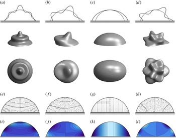
Figure 4 shows example modes with mobile contact lines for
 ${\it\alpha}=75^{\circ }$
to illustrate (a–d) interface shapes, (e–h) streamlines and (i–l) velocity potentials (pressure). Interface shapes are shown in longitudinal section (a–d), perspective view (e–h) and top view (i–l). The nodal lines for the
 $[8,0]$
zonal mode (a) consist of four latitudinal circles, whereas the
 $[2,2]$
sectoral mode (c) has two longitudinal circles (most readily seen in latitudinal section). The remaining tesseral modes, (b)
 $[5,1]$
and (d)
 $[7,3]$
, respect the prescription for
 $(k-l)/2$
latitudinal and
 $l$
longitudinal nodal circles.
Eigenmodes: (a,e,i) zonal
 $[k,l]=[8,0]$
, (b, f,j) lateral
 $[k,l]=[5,1]$
, (c,g,k) sectoral
 $[k,l]=[2,2]$
and (d,h,l) tesseral
 $[k,l]=[7,3]$
modes illustrating the (a–d) disturbed interface, (e–h) streamlines and (i–l) velocity potential (pressure) for a subhemispherical drop
 ${\it\alpha}=75^{\circ }$
with mobile contact lines. Here, the dashed (dotted) curves in (e–h) denote points of zero horizontal (vertical) velocity. The drop surface in (e–l) is unperturbed.

It turns out that the
 $l=1$
modes are especially easy to identify in experiments since their one sector rocks from side to side. These ‘rocking’ modes are illustrated by the
 $[5,1]$
mode in figure 4(b). During an oscillation, its peak moves down, across and up again, as it rocks from one side to the other side, much like a seventies disco move. It should be noted that the Noether mode (
 $[1,1]$
), defined in § 1, is a special rocking mode.
In order to more easily identify tesseral modes in experiments, Chang et al. (Reference Chang, Bostwick, Steen and Daniel2013) have introduced an alternative scheme based on ‘layers’
 $n$
and ‘sectors’
 $l$
with
 $n=(k-l)/2+1$
. These are most easily seen in top view. For example, the mode shown in figure 4(d) has three sectors and three layers, yielding
 $(n,l)=(3,3)$
. Alternatively, figure 4(b) shows a mode with one sector and three layers, corresponding to
 $(n,l)=(3,1)$
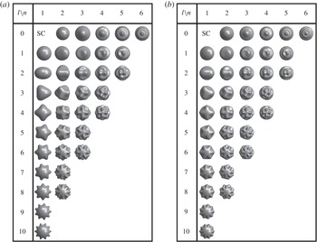
. Sectoral modes have one layer and zonals have zero sectors. A video tutorial for this classification scheme can be found in Chang (Reference Chang2013). Figures 5(a,b) use the layer/sector classification and show the first 35 modes, contrasting natural modes for (a)
 ${\it\alpha}=90^{\circ }$
(RL modes) and (b) pinned modes with
 ${\it\alpha}=75^{\circ }$
. The differences appear minor, but are most clearly seen near the contact line, where the interface shape adjusts itself to accommodate the pinned contact-line condition. The ability to model wetting properties is one reason why our predictions have been able to accurately capture recent experiments on sessile drop vibrations (Chang et al.
Reference Chang, Bostwick, Steen and Daniel2013). In Chang et al. (Reference Chang, Bostwick, Daniel and Steen2014), we demonstrate the utility of our model over a wide range of contact angles.
Sector (
 $l$
)–layer (
 $n$
) table of rendered mode shapes (top view): (a) RL modes (
 ${\it\alpha}=90^{\circ }$
, free contact line), which reorganize and extend figure 2, compared with (b) a sessile drop with
 ${\it\alpha}=75^{\circ }$
and a pinned contact line. Here,
 $l$
is the azimuthal wavenumber and
 $n\equiv (k-l)/2+1$
is the number of layers, with
 $k$
the standard polar wavenumber; SC
 $=$
spherical cap.

The streamlines, illustrated in figures 4(e–h), show velocities with vertical and horizontal components. The motions of the sectoral mode (g) are purely horizontal while those of the zonal mode (e) are strongly vertical. It turns out that the predominantly horizontal or vertical character of the motion correlates with the influence of support on the modal frequency. That is, the frequencies of the sectoral mode are only slightly affected by the volume (equivalently
 ${\it\alpha}$
) while those of the zonal mode are strongly affected. Vertical motion, alternatively, correlates with the number of layers
 $n$
. In summary, larger
 $n$
modes are more sensitive to the presence of support, as measured by the frequency slope.
Additionally correlating with the horizontal/vertical motion of a natural mode is the displacement at the contact line. Horizontal motion favours, while vertical motion inhibits, contact-line displacement. In figures 4(a–d), top row, the four plots all have the same maximum deviation amplitude from the spherical cap. However, that maximum occurs at different places around the cap. The
 $[2,2]$
sectoral mode (c) exhibits a larger excursion than the
 $[8,0]$
zonal mode (a), while the rocking
 $[5,1]$
(b) and tesseral
 $[7,3]$
(d) modes have intermediate displacements. In summary, the number of layers correlates with both streamline (horizontal/vertical) motion and contact-line excursion.
7. Results for kinematic disturbances:
${\it\alpha}$
dependence

7.1. Axisymmetric
$(l=0)$
modes

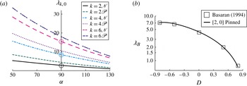
Figure 6(a) plots the frequency
 ${\it\lambda}_{k,0}$
against the contact angle
 ${\it\alpha}$
for the axisymmetric (
 $l=0$
) modes. Frequencies for the natural (
 $\mathscr{N}$
) and pinned (
 $\mathscr{P}$
) modes are shown paired. For the hemispherical drop, the natural modes are precisely the RL modes with associated frequency, identified by circles, while the corresponding pinned modes shift to higher frequency. These frequencies reproduce the summary in figures 2(a,b), respectively. The fact that the pinned frequency is always higher than the natural frequency is a result of the restriction that pinning places on the function space of disturbances. As with many classical problems in mathematical physics, such as the vibrating drum head, more constrained function spaces lead to uniformly higher frequencies (Courant & Hilbert Reference Courant and Hilbert1953).
Zonal modes (
 $l=0$
). (a) Frequency
 ${\it\lambda}_{k,0}$
against contact angle
 ${\it\alpha}$
for the natural
 $\mathscr{N}$
and pinned
 $\mathscr{P}$
disturbances. The RL frequencies are circled. (b) Frequency
 ${\it\lambda}_{B}$
against shape parameter
 $D=-\text{cos}{\it\alpha}$
for finite-element simulations (symbols) (Basaran & DePaoli Reference Basaran and DePaoli1994, figure 7) and pinned
 $[2,0]$
predictions (solid line) (this work).

Figure 6(a) shows that frequencies break from the hemisphere by increasing for lens-like and decreasing for drop-like caps. This is a consequence of the lesser (greater) volume of the lens-like (drop-like) shape which implies lesser (greater) inertia. Another noteworthy feature of figure 6(a) is the convergence of frequencies as
 ${\it\alpha}$
gets larger. Indeed, all the frequencies limit to zero as
 ${\it\alpha}\rightarrow 180^{\circ }$
. This occurs because, in the limit of the drop touching the support plane at a single point, the natural disturbance degenerates into the pinned disturbance. Moreover, this limit corresponds to infinite volume and hence all the modal frequencies approach zero, related to our scaling. It should be noted that the spectral ordering established for the RL modes is maintained for all
 ${\it\alpha}$
. That is, any zonal mode can be related back uniquely to a RL mode.
The relative frequency difference
 $({\it\lambda}_{p}-{\it\lambda}_{n})/{\it\lambda}_{p}$
between the natural (
 ${\it\lambda}_{n}$
) and pinned (
 ${\it\lambda}_{p}$
) disturbances measures the ‘degree-of-pinning’ of a contact line. A small relative difference in frequency indicates that the contact line is essentially pinned and one cannot distinguish between the natural and pinned disturbances. For example, consider the hemispherical drop (
 ${\it\alpha}=90^{\circ }$
) and compare the relative frequency difference of 11 % for the
 $[6,0]$
mode with the 42 % difference for the
 $[2,0]$
mode (cf. figure 6). One concludes that the
 $[6,0]$
mode has a much smaller contact-line displacement than the
 $[2,0]$
mode. For the natural disturbance, the contact-line degree-of-pinning is greatly influenced by the polar wavenumber
 $k$
.
Finally, regarding validation against prior work, figure 6(b) replots the pinned
 $[2,0]$
frequencies (solid line) in a form compatible with Basaran & DePaoli (Reference Basaran and DePaoli1994). They report finite-element simulations (symbols) for drop vibrations over a range of parameters that include the variable wetting properties of the solid substrate. The comparison is reasonable. We also reproduce the zonal frequencies for the limiting cases
 ${\it\Lambda}=0,\infty$
predicted by Lyubimov et al. (Reference Lyubimov, Lyubimova and Shklyaev2006, table I) for a hemispherical drop. More recently, experiments by Chang et al. (Reference Chang, Bostwick, Steen and Daniel2013) have been reported which measure a range of zonal frequencies,
 $k=2,4,6,8,10,12,14$
, for pinned drops with
 ${\it\alpha}\sim 70^{\circ }$
. They show conclusively that the RL frequency predictions are inadequate, while our predictions are consistent with observation (Chang et al.
Reference Chang, Bostwick, Steen and Daniel2013, figure 6a,d).
7.2. Rocking
$(l=1)$
modes

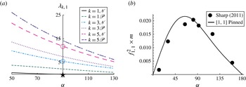
Figure 7(a) plots the frequency
 ${\it\lambda}_{k,1}$
against the contact angle
 ${\it\alpha}$
for the rocking (
 $l=1$
) modes. Again, frequencies of natural (
 $\mathscr{N}$
) and pinned (
 $\mathscr{P}$
) modes are paired. For the hemisphere (
 ${\it\alpha}=90^{\circ }$
), the
 $[1,1]$
natural mode is the Noether mode (
 $\star$
), while the
 $[3,1]$
and
 $[5,1]$
natural modes are the RL modes (○). As for the zonals, the pinned frequencies are shifted upwards from the natural frequencies, and for the same reason. The frequencies all break similarly from the hemisphere, increasing (decreasing) for smaller (greater)
 ${\it\alpha}$
because of decreasing (increasing) inertia due to volume.
The
 $l=1$
spectrum. (a) Scaled frequency
 ${\it\lambda}_{k,1}$
against contact angle
 ${\it\alpha}$
for the natural
 $\mathscr{N}$
and pinned
 $\mathscr{P}$
disturbances. Here,
 $\text{Im}[{\it\lambda}_{k,1}]=0$
in all cases except for
 $k=1\mathscr{N}$
,
 ${\it\alpha}>90^{\circ }$
(cf. figure 8
a). RL frequencies are denoted by ○ and the Noether mode by
 $\star$
. (b) Comparison between experiments (Sharp et al.
Reference Sharp, Farmer and Kelly2011, figure 3) and the
 $[1,1]$
pinned mode by plotting
 $f_{1,1}^{2}\times m$
against
 ${\it\alpha}$
, where
 $f$
is the real frequency and
 $m$
is the mass of the droplet.

The hemispherical Noether mode (
 $\star$
) has zero frequency. That the oscillation frequency is exactly zero is important and we sketch the proof. To begin, the function
 $P_{1}^{(1)}(x)$
is a fundamental solution of the curvature operator (3.3b
) and uniquely satisfies the natural boundary conditions (3.8) for the hemispherical base state. Therefore, this function belongs to the kernel of (3.3b
). It is also straightforward to show that the ‘inertia’ operator (3.3a
) is positive definite. Thus, applying the Fredholm alternative for linear operators to this particular mode shape delivers
 ${\it\lambda}_{1,1}^{2}=0$
. The motion of the
 $\star$
mode corresponds to a horizontal translation of the drop’s centre-of-mass. This motion is analogous to the zero-frequency mode of the drop pinned on an equatorial circle-of-contact (Bostwick & Steen Reference Bostwick and Steen2009) and likewise can be attributed to the additional symmetry inherent in the hemispherical base state (Field, Golubitsky & Stewart Reference Field, Golubitsky and Stewart1991), as outlined in § 1.
The Noether frequency squared,
 ${\it\lambda}_{1,1}^{2}$
, breaks higher for lens-like base states, yielding a shift upwards as for the other rocking modes. In the direction of drop-like shapes, it breaks to
 ${\it\lambda}_{1,1}^{2}<0$
, also consistent with higher rocking modes. The important difference is that the break is from zero which puts it in negative territory. Exponential growth results, according to (2.12). Hence, the walking instability may be anticipated by the symmetry breaking of the RL Noether mode. It should be noted that figure 7(a) plots the real part of
 ${\it\lambda}_{1,1}$
.
Finally, regarding validation against prior work, figure 7(b) replots the pinned
 $[1,1]$
frequencies (solid line) in the form that Sharp et al. (Reference Sharp, Farmer and Kelly2011) report their experiments. Figure 7(b) reports the observed oscillation frequency
 $f_{1,1}$
against the contact angle
 ${\it\alpha}$
(symbols). The pinned drop experiments (
 ${\it\alpha}\sim 70^{\circ }$
) of Chang et al. (Reference Chang, Bostwick, Steen and Daniel2013) also measure the frequencies of several rocking modes,
 $k=1,3,5,7,9$
, with reasonable comparison (Chang et al.
Reference Chang, Bostwick, Steen and Daniel2013, figures 6, 13, 14).
7.2.1. Noether mode: ‘walking’ droplet instability
The sessile drop exhibits instability (
 ${\it\lambda}^{2}<0$
) to the natural disturbance for drop-like base states; that is, those in the range of contact angles
 $90^{\circ }<{\it\alpha}<180^{\circ }$
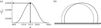
. Figure 8(a) plots the square of the instability growth rate
 $-{\it\lambda}_{1,1}^{2}$
against the static contact angle
 ${\it\alpha}$
. It shows that the maximum growth rate (
 $-{\it\lambda}_{1,1}^{2}=0.0458$
) occurs at
 ${\it\alpha}=132.5^{\circ }$
. A typical unstable mode shape is shown in figure 8(b).
The
 $[k,l]=[1,1]$
instability: (a) instability growth rate
 $-{\it\lambda}_{1,1}^{2}$
against contact angle
 ${\it\alpha}$
and (b) a typical instability mode shape with contact angle
 ${\it\alpha}=120^{\circ }$
in polar view.

Insight into the instability mechanism is gained by evaluating the static free energy functional
 $U$
at the mode shape
 $y_{1,1}$
. The idea is that the instability will occur when the perturbed state has a lower energy than the base state. For a fully mobile sessile drop of contact angle
 ${\it\alpha}$
, we define
 $U$
for a general capillary surface
 $\boldsymbol{x}(u,v)$
,
 $$\begin{eqnarray}U/{\it\sigma}_{lg}=\int _{{\it\Gamma}}|\boldsymbol{x},_{u}\times \,\boldsymbol{x},_{v}|\text{d}{\it\Gamma},\end{eqnarray}$$
where
 $u,v$
are surface coordinates. We then take the second variation of the potential energy (Myshkis et al.
Reference Myshkis, Babskii, Slobozhanin and Tyuptsov1987),
 $$\begin{eqnarray}{\it\delta}^{2}U=-\int _{b}^{1}\left[\left(\left(1-x^{2}\right)y^{\prime }\right)^{\prime }+\left(2-\frac{1}{1-x^{2}}\right)y\right]y\,\text{d}x,\end{eqnarray}$$
and integrate by parts using the natural boundary condition (3.8) to obtain
 $$\begin{eqnarray}{\it\delta}^{2}U=\int _{b}^{1}\left[\left(1-x^{2}\right)\left(y^{\prime }\right)^{2}-\left(2-\frac{1}{1-x^{2}}\right)y^{2}\right]\text{d}x+b\,\sqrt{1-b^{2}}\,y^{2}(b).\end{eqnarray}$$
This equivalent form of the total disturbance energy
 $E_{t}$
may be decomposed into two interfacial energies (
 $E_{1},E_{2}$
) and one contact-line energy (
 $E_{3}$
),
 $$\begin{eqnarray}\displaystyle E_{t} & = & \displaystyle E_{1}+E_{2}+E_{3},\end{eqnarray}$$
 $$\begin{eqnarray}\displaystyle E_{1} & \equiv & \displaystyle \int _{b}^{1}\left(1-x^{2}\right)\left(y^{\prime }\right)^{2}\text{d}x,\end{eqnarray}$$
 $$\begin{eqnarray}\displaystyle E_{2} & \equiv & \displaystyle -\int _{b}^{1}\left(2-\frac{1}{1-x^{2}}\right)y^{2}\text{d}x,\end{eqnarray}$$
 $$\begin{eqnarray}\displaystyle E_{3} & \equiv & \displaystyle b\,\sqrt{1-b^{2}}\,y^{2}(b).\end{eqnarray}$$
 $E_{1}$
is a positive-definite (stabilizing) measure of the gradients in the mean curvature of the perturbed surface, while
 $E_{2}$
represents the tendency of a volume of liquid to form an isolated spherical drop (minimal energy state). In contrast, the contact-line energy
 $E_{3}$
can either stabilize (
 $E_{3}>0$
) or destabilize (
 $E_{3}<0$
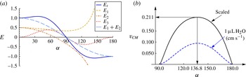
), depending upon the geometry of the base state. Figure 9(a) plots the decomposition of the disturbance energy, showing that for the range of base states that exhibit instability,
 $90^{\circ }<{\it\alpha}<180^{\circ }$
, the droplet reduces its energy by lowering the interfacial (
 $E_{1}+E_{2}$
) and contact-line (
 $E_{3}$
) energies.
Energetics for the walking instability: (a) decomposition of the disturbance energy (
 $E$
) and (b) scaled walking speed
 $v_{CM}$
(solid line), evaluated in
 $\text{cm}\ \text{s}^{-1}$
for a
 $1\ {\rm\mu}\text{L}$
drop of water (dashed line) using the velocity scale
 $v\sqrt{{\it\rho}r/{\it\sigma}}$
.

The reduction in energy drives fluid motion, which is shown to correlate with horizontal motion of the centre-of-mass. Hence, we refer to the instability as the ‘walking’ droplet instability. A standard calculation of the horizontal centre-of-mass
 $\bar{x}(t)=\int x(t)\text{d}V/\int \text{d}V$
of the disturbed interface shape
 $y(s)$
shows that the instantaneous walking speed
 $v_{CM}\equiv \dot{\bar{x}}(t=0)$
is given by
 $$\begin{eqnarray}v_{CM}=\sqrt{-{\it\lambda}^{2}}\frac{3\displaystyle \int _{0}^{{\it\alpha}}y(s)\sin ^{2}s\text{d}s}{2\left(1-\cos {\it\alpha}\right)\sin {\it\alpha}}.\end{eqnarray}$$
Figure 9(b), which plots the walking speed
 $v_{CM}$
against the static contact angle
 ${\it\alpha}$
, shows that the maximum walking speed (
 $v_{CM}=0.211$
) occurs at
 ${\it\alpha}=136.8^{\circ }$
. For reference, we evaluate (7.5) for a
 $1\ {\rm\mu}\text{L}$
drop of water (
 $\text{H}_{2}\text{O}$
) and plot against
 ${\it\alpha}$
.
7.3. Azimuthal
$(l\neq 0)$
modes

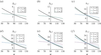
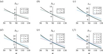
For natural and pinned disturbances, respectively, figures 10 and 11 show how the azimuthal modes break the hemispherical base-state degeneracy (cf. figures 2
a,c). Zonal
 $l=0$
modes are included for reference. For fixed mode shape, in all cases, the frequency decreases monotonically with increasing volume (increasing
 ${\it\alpha}$
) since higher inertia (volume) biases toward lower frequencies, just as for the zonal modes discussed above. For natural and pinned disturbances, this negative slope decreases with higher mode number
 $l$
relative to the reference mode, zonal
 $l=0$
or rocking
 $l=1$
. The least slope coincides with the sectoral mode, the highest azimuthal wavenumber possible. That is, for the natural disturbances, the frequencies of drop-like volumes break upward while those for lens-like volumes break downward, relative to the reference mode (figure 10). The net effect is a plot that looks like a bowtie, only with a skew. For the pinned disturbances, the frequencies behave similarly, only with the centre of the bowtie shifted to lower volumes (figure 11).
Natural disturbance: frequency
 ${\it\lambda}_{k,l}$
, as it depends upon azimuthal wavenumber
 $l$
, against contact angle
 ${\it\alpha}$
for fixed polar wavenumber (a)
 $k=2$
, (b)
 $k=3$
, (c)
 $k=4$
, (d)
 $k=5$
, (e)
 $k=6$
and (f)
 $k=7$
. It should be noted that the scaling of the frequency is different for (a)–(f).

Pinned disturbance: frequency
 ${\it\lambda}_{k,l}$
, as it depends upon azimuthal wavenumber
 $l$
, against contact angle
 ${\it\alpha}$
for fixed polar wavenumber (a)
 $k=2$
, (b)
 $k=3$
, (c)
 $k=4$
, (d)
 $k=5$
, (e)
 $k=6$
and (f)
 $k=7$
. It should be noted that the scaling of the frequency is different for (a)–(f).

In summary, the new feature of this degeneracy breaking is that, for the same polar wavenumber
 $k$
, higher azimuthal wavenumber
 $l$
modes can have lower frequencies. This occurs because the influence of the support, as measured by the relative slope of frequency with
 ${\it\alpha}$
, increases with increasing number of layers
 $n$
, as discussed above. There is one volume for which the shape is indifferent to horizontal and vertical motions. That is, all frequencies must pass through a centre. For natural disturbances, this centre is the hemispherical shape while, for pinned disturbances, the centre shifts to a lens-like shape. This shift can be understood as pinning being more inhibiting to motions of a horizontal than a vertical nature. Together, these two factors explain why the sectoral mode frequencies are lowest for lens-like and highest for drop-like shapes. Stated differently, the mode with least vertical motion has the lowest frequency for lens-like shapes while that with the greatest vertical motion has the lowest frequency for drop-like shapes. The relative frequency difference between the zonal (
 $l=0$
) and sectoral (
 $l=k$
) modes can be large. For example, the difference between the
 $[4,0]$
and
 $[4,4]$
modes approaches 100 % for the lens-like base state
 ${\it\alpha}=50^{\circ }$
(cf. figure 10
c). Finally, for a fixed polar wavenumber
 $k$
, the frequency difference for the pinned disturbance is much smaller than that for the natural disturbance (e.g. figures 10
a, 11
a). Pinning inhibits motion, lessening frequency differences.
Comparison of these predictions against the pinned drop experiments (
 ${\it\alpha}\sim 70^{\circ }$
) of Chang et al. (Reference Chang, Bostwick, Steen and Daniel2013, figure 14d), who measure the frequencies of several tesseral modes,
 $[6,2]$
,
 $[7,3]$
,
 $[8,4]$
,
 $[9,5]$
,
 $[10,6]$
, are found to be reasonable.
7.4. Frequency crossings:
${\it\alpha}$
dependence

Up to now, spectral ordering has been preserved in every case discussed. Across all
 ${\it\alpha}$
, pinned and natural zonals respect the spectral ordering of the RL modes (cf. figures 6
a,b), as do pinned and natural rocking modes (cf. figure 7
a). Moreover, for the other natural tesseral modes, spectral ordering in
 $l$
(fixed
 $k$
) is preserved for
 ${\it\alpha}>90^{\circ }$
while a reverse spectral ordering is seen for
 ${\it\alpha}<90^{\circ }$
, as shown in figure 10. For the other pinned tesseral modes, a spectral (or reverse spectral) ordering is nearly respected (cf. figure 11). The preservation or not of spectral ordering is related to the Sturm–Liouville nature of the operator (3.1). In general, zonal and azimuthal modes must both be considered in which case spectral ordering will be the exception.
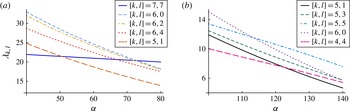
Figure 12 illustrates two examples where spectral ordering is broken, one for lens-like and the other for drop-like shapes. Consistent with the influence of inertia, all frequencies decay monotonically with
 ${\it\alpha}$
but with different slopes depending on the horizontal/vertical motion of associated modes. A necessary condition for crossing is that modes of different
 $k$
compete. In figure 12(a), polar wavenumbers
 $k=5,6$
and
 $k=7$
are represented. Three different
 $k=6$
modes are included and none of these frequencies can cross, by spectral ordering. On the other hand, the rocking
 $[5,1]$
and sectoral
 $[7,7]$
could cross the
 $k=6$
modes (and/or each other). The sectoral mode, with its predominantly horizontal motions, has the weakest slope and greatest relative difference in slopes; this may be viewed as the active mode in crossing the others, yielding four crossings in total. Figure 12(b) likewise includes five modes: two sectorals, one rocking and three with the same
 $k$
. Here, the ‘loner’ sectoral
 $[4,4]$
has the weakest slope and crosses the rocking mode. The other sectoral
 $[5,5]$
is also active and crosses the
 $[6,0]$
zonal. A total of two crossings are seen in the range of
 ${\it\alpha}$
plotted. Experiments reported in Chang et al. (Reference Chang, Bostwick, Daniel and Steen2014) test such predictions.
Frequency crossings controlled by base-state volume: frequency
 ${\it\lambda}_{k,l}$
as a function of static contact angle
 ${\it\alpha}$
for (a) natural and (b) pinned disturbances.

8. Method for dynamic disturbances: mobile contact lines
In principle, the inverse method could be used to satisfy the dynamic contact-line condition (3.11), but this formulation gives rise to an integral operator with the eigenvalue parameter in its kernel, which is notorious for computational instability (e.g. Walter Reference Walter1973). To circumvent this issue, we solve the direct problem by utilizing results for the natural disturbance and exploiting the variational structure associated with (3.1).
8.1. Contact-line energy
To begin, consider the second variation of the surface energy
 $U$
, equivalent to, but in a form more general than, (7.1),
 $$\begin{eqnarray}{\it\delta}^{2}U=-\int _{{\it\Gamma}}\left(\left({\it\kappa}_{1}^{2}+{\it\kappa}_{2}^{2}\right)\frac{\partial {\it\phi}}{\partial n}+{\it\Delta}_{{\it\Gamma}}\frac{\partial {\it\phi}}{\partial n}\right)\frac{\partial {\it\phi}}{\partial n}\text{d}{\it\Gamma}+\int _{{\it\zeta}}\left(\frac{\partial }{\partial s}\left(\frac{\partial {\it\phi}}{\partial n}\right)+\cos ({\it\alpha})\frac{\partial {\it\phi}}{\partial n}\right)\frac{\partial {\it\phi}}{\partial n}\text{d}{\it\zeta},\end{eqnarray}$$
with contributions from the free surface
 ${\it\Gamma}$
and contact line
 ${\it\zeta}$
(Myshkis et al.
Reference Myshkis, Babskii, Slobozhanin and Tyuptsov1987). The corresponding boundary-value problem for the hydrodynamic problem is given by the integrodifferential equation (3.1) combined with a boundary condition on the three-phase contact line. As is evident from (8.1), there is no contact-line energy associated with the natural (3.8) or pinned (3.9) disturbances. In contrast, applying the dynamic contact-line condition (3.11) to (8.1) results in an associated contact-line energy,
 $\text{i}{\it\lambda}{\it\Lambda}\int _{{\it\zeta}}(\partial {\it\phi}/\partial n)^{2}\text{d}{\it\zeta}$
, whose form demonstrates that contact-line motion is dissipative. To distinguish this effective dissipation from viscous dissipation, we shall refer to it as ‘Davis’ dissipation, first identified by Davis (Reference Davis1980).
To proceed with our solution technique, we recall two results from the calculus of variations: (i) the natural disturbance is the absolute minimizer and (ii) the pinned disturbance is the absolute maximum of the minimizers of the second variation of the surface energy (8.1) (Courant & Hilbert Reference Courant and Hilbert1953). That is, applying the natural (pinned) boundary condition to the operator (3.1) results in the smallest (largest) possible disturbance energy. We exploit (i) in formulating the solution method for the dynamic contact-line disturbance.
8.2. Computational evaluation: hybrid Rayleigh–Ritz
We compute the spectrum for the dynamic contact-line disturbance by solving the direct problem (3.2). We recall that for the direct problem the unknown function in the Rayleigh–Ritz procedure is the interface disturbance and one must compute the associated velocity potential. As stated earlier, this proves to be a daunting task for most geometries, including the spherical-cap geometry used here. However, judicious choice of the function space in the Rayleigh–Ritz method can circumvent this difficulty associated with an ab initio solution of the direct problem. We choose the complete set of natural mode shapes
 $y_{j,l}$
, defined in (4.21), as the basis functions in the requisite solution series
 $$\begin{eqnarray}\frac{\partial {\it\phi}^{(l)}}{\partial n}=\mathop{\sum }\limits_{j=1}^{N}c_{j}y_{j,l}(x),\end{eqnarray}$$
where
 $l$
is the azimuthal wavenumber.
To explain our choice of function space, we recall that solution of the inverse problem (3.5) results in eigenfunctions (4.20) identified as velocity potentials
 ${\it\phi}$
, which are related to the interface disturbance
 $y\propto \partial {\it\phi}/\partial n$
(4.21). Hence, this solves precisely the difficulty with the direct problem (3.2) in a relatively simple manner. Finally, we choose the natural mode shapes as the basis functions (8.2) because they span the least restrictive function space (see Courant & Hilbert Reference Courant and Hilbert1953; Lanczos Reference Lanczos1986; Segel Reference Segel1987) and solve a limiting case (
 ${\it\Lambda}=0$
) of the dynamic contact-line condition (3.11). It should be noted that the pinned contact-line disturbance, limiting case (
 ${\it\Lambda}\rightarrow \infty$
) of (3.11), can be recovered from the natural disturbance using any number of solution techniques (e.g. Lyubimov et al.
Reference Lyubimov, Lyubimova and Shklyaev2006; Bostwick & Steen Reference Bostwick and Steen2010; Prosperetti Reference Prosperetti2012). In contrast, the natural disturbance cannot be recovered from the pinned disturbance.
Finally, we apply the solution series (8.2) to the direct problem (3.2), resulting in the following set of algebraic equations:
 $$\begin{eqnarray}\mathop{\sum }\limits_{j=1}^{N}\left[\unicode[STIX]{x1D612}_{ij}^{(l)}+\frac{\text{i}{\it\lambda}}{\sqrt{1-b^{2}}}{\it\Phi}_{ij}^{(l)}+\frac{{\it\lambda}^{2}}{1-b^{2}}\unicode[STIX]{x1D614}_{ij}^{(l)}\right]c_{j}=0,\end{eqnarray}$$
with matrix elements
 $$\begin{eqnarray}\displaystyle & \displaystyle \unicode[STIX]{x1D612}_{ij}^{(l)}\equiv \int _{b}^{1}\left(\left(1-x^{2}\right)\left(y_{i,l}\right)_{xx}-2x\left(y_{i,l}\right)_{x}+\left(2-\frac{l^{2}}{1-x^{2}}\right)y_{i,l}\right)y_{j,l}\text{d}x, & \displaystyle\end{eqnarray}$$
 $$\begin{eqnarray}\displaystyle & \displaystyle {\it\Phi}_{ij}^{(l)}\equiv {\it\Lambda}\;y_{i,l}(b)y_{j,l}(b), & \displaystyle\end{eqnarray}$$
 $$\begin{eqnarray}\displaystyle & \displaystyle \unicode[STIX]{x1D614}_{ij}^{(l)}\equiv \int _{b}^{1}{\it\phi}_{i,l}y_{j,l}\text{d}x. & \displaystyle\end{eqnarray}$$
 ${\it\Lambda}$
in (8.4b
) is dissipative.
The complex frequencies
 ${\it\lambda}=-{\it\gamma}+\text{i}{\it\omega}$
, as they depend upon the static contact angle
 ${\it\alpha}$
and spreading parameter
 ${\it\Lambda}$
, are computed from the characteristic equation associated with the matrix (8.3). Computations show that a truncation of
 $N=12$
terms in the solution series (8.2) is sufficient to generate relative eigenvalue convergence of 0.1 % for the results presented here. For a given eigenvalue
 ${\it\lambda}_{k,l}$
, the mode shapes corresponding to the eigenvector
 $c_{j}^{(k,l)}$
with polar
 $k$
and azimuthal
 $l$
wavenumbers are given by
 $$\begin{eqnarray}{\it\psi}_{k,l}=\mathop{\sum }\limits_{j=1}^{N}c_{j}^{(k,l)}y_{j,l}.\end{eqnarray}$$
9. Results for dynamic disturbances:
${\it\Lambda}$
dependence

9.1. Davis dissipation
The spreading parameter
 ${\it\Lambda}$
is a measure of the resistance of a contact line to spreading that can change the disturbance from natural
 $({\it\Lambda}\rightarrow 0)$
to pinned
 $({\it\Lambda}\rightarrow \infty )$
. Here,
 ${\it\Lambda}$
is also a measure of the Davis dissipation (8.4b
), an irrecoverable loss that results from the dynamic contact-line condition (3.11) and leads to damping of oscillations
 ${\it\gamma}>0$
. Here, one should note that the decay rate scales with the capillary frequency (2.13f
). In comparison, for an isolated spherical drop, the decay rate from viscous dissipation scales with the viscosity
 ${\it\nu}$
as
 ${\it\gamma}_{k,l}={\it\nu}/R^{2}\,(k-1)(2k+1)$
(Lamb Reference Lamb1932).
One can use the damped-harmonic oscillator structure of (8.3) and related formalism (e.g. Taylor Reference Taylor2005, § 5.6) to define the Davis dissipation over an oscillation cycle as
 $$\begin{eqnarray}Q_{k,l}\equiv 2{\rm\pi}\frac{{\it\gamma}_{k,l}}{{\it\omega}_{k,l}}.\end{eqnarray}$$
This is commonly referred to as the
 $Q$
-factor. For reference, for an isolated spherical drop, the effective dissipation due to bulk viscous effects is given by
 $Q_{k,l}\propto \sqrt{k}$
.
The influence of
 ${\it\Lambda}$
on the frequency is illustrated for zonals in figure 13 and for azimuthal modes in figure 14. The plots show a step-like function increase in frequency from natural to pinned disturbances. This monotonic increase is consistent with increasing constraint. Figures 13(a,d,g) show that the spectral ordering at
 ${\it\Lambda}=0$
and
 ${\it\Lambda}=\infty$
noted for zonals is maintained. The plots in figures 13(b,e,h) illustrate that the decay rate also maintains spectral ordering over the
 ${\it\Lambda}$
range. Starting from
 ${\it\Lambda}=0$
, the decay rate rises to reach a maximum at a finite value of
 ${\it\Lambda}$
and then tends back to zero for large
 ${\it\Lambda}$
. Figures 13(c,f,i) show that the low-wavenumber modes have the largest dissipation per cycle. This can be directly attributed to the contact-line displacement, which is more pronounced for the lower polar wavenumber modes. Since Davis dissipation (8.4b
) is related to contact-line displacement, the low-wavenumber modes might be expected to dissipate the most per cycle. Furthermore, it has been established in § 7.1 that the maximum displacement of the contact line decreases as the static contact angle increases. Figures 13(c,i) compare the dissipation per cycle for lens-like (
 ${\it\alpha}=75^{\circ }$
) and drop-like (
 ${\it\alpha}=105^{\circ }$
) shapes, respectively. Unsurprisingly, the lens-like modes dissipate more energy, as their contact lines show greater displacement. For these comparisons, recall that the disturbance kinetic energy is normalized via the denominator in the Rayleigh–Ritz quotient.
Complex frequency for zonal (
 $l=0$
) modes: (a,d,g) oscillation frequency
 ${\it\omega}_{k,0}$
, (b,e,h) decay rate
 ${\it\gamma}_{k,0}$
and (c,f,i) Davis dissipation
 $Q_{k,0}$
as a function of the spreading parameter
 ${\it\Lambda}$
for an (a–c) sub-hemispherical (
 ${\it\alpha}=75^{\circ }$
), (d–f) hemispherical (
 ${\it\alpha}=90^{\circ }$
) and (g–i) super-hemispherical (
 ${\it\alpha}=105^{\circ }$
) drop.

Complex frequency for the
 $k=6$
modes: (a) oscillation frequency
 ${\it\omega}_{6,l}$
, (b) decay rate
 ${\it\gamma}_{6,l}$
and (c) and effective dissipation
 $Q_{6,l}$
as a function of the spreading parameter
 ${\it\Lambda}$
for contact angle
 ${\it\alpha}=105^{\circ }$
.

For azimuthal modes with
 ${\it\alpha}=105^{\circ }$
, figure 14(a) shows that spectral ordering is maintained over the range of
 ${\it\Lambda}$
. For azimuthal modes with small
 ${\it\alpha}$
, reverse spectral ordering is maintained (not shown), consistent with the bowtie structure for natural (cf. figure 10
e) and pinned (cf. figure 11
e) disturbances. Moreover, for a fixed polar wavenumber
 $k$
, the mode of maximal dissipation has either the largest or the smallest possible azimuthal wavenumber for the lens-like and drop-like base states, respectively. However, changes in spectral ordering and the variation in position of the step change in frequency (cf. figure 14
a) accommodate
 ${\it\Lambda}$
-crossings, discussed below in § 9.3. For similar reasons, the mode that dissipates the largest amount of energy per cycle may change at different values of the spreading parameter. For example, figure 14(c) shows that for fixed spreading parameters
 ${\it\Lambda}=0.5$
and
 ${\it\Lambda}=1$
, the
 $[6,4]$
and
 $[6,2]$
modes have the largest effective dissipation, respectively. However, the mode with maximal effective dissipation over the entire range of spreading parameters is predicted by the geometry of the base state: high (low) azimuthal wavenumber modes for lens-like (drop-like) base states.
9.2. Dissipative Noether mode: onset of ‘walking’
Davis dissipation from the dynamic contact-line condition can suppress the walking droplet instability (cf. figure 8). Figure 9 shows that the disturbance energy for the
 $[1,1]$
natural mode is lower than the base-state energy, resulting in instability. The effective dissipation from the dynamic contact-line condition (8.4b
),
 $$\begin{eqnarray}E_{d}={\it\Lambda}\left(y_{1,1}(b)\right)^{2},\end{eqnarray}$$
can counteract the net energy gained in going from the base to the disturbed state (
 $E_{t}$
) (7.4). The base state is neutrally stable when the dissipation exactly balances the disturbance energy (
 $E_{d}=E_{t}$
). This criterion is used to determine the onset of ‘droplet walking’, as plotted in figure 15. In the limit
 ${\it\alpha}\rightarrow 180^{\circ }$
, the instability window remains open despite the small instability growth rate observed in this limit (cf. figure 8
a). Here, the stabilizing dissipation
 $E_{d}\rightarrow 0$
because the contact-line displacement is small,
 $y_{1,1}(\mathit{b})\rightarrow 0$
. Hence, a large
 ${\it\Lambda}_{c}$
can be overcome by a small destabilizing disturbance energy (
 $E_{t}<0$
), as shown in figure 9(a). With regards to growth rate, the effective dissipation is a monotonically increasing function of the spreading parameter
 ${\it\Lambda}$
; therefore, the maximum instability growth rate corresponds to the natural disturbance
 ${\it\Lambda}=0$
, as shown in figure 8(a).
Onset of walking for the
 $[k,l]=[1,1]$
mode: for fixed
 ${\it\alpha}$
, on decreasing
 ${\it\Lambda}$
, rocking turns to walking across a critical value (solid line).

9.3. Frequency crossings:
${\it\Lambda}$
dependence

As discussed in § 7.1, spectral ordering is maintained for zonals. More generally, spectral ordering is respected for families of fixed
 $k$
, as seen in figure 16(a) for the four
 $k=7$
modes. In contrast, crossings become typical when a different
 $k$
is introduced, as with
 $[8,0]$
in figure 16. We count five crossings amongst the
 $[8,0]$
and
 $[7,3]$
,
 $[7,5]$
and
 $[7,7]$
modes. Frequency crossings correspond to multiplicity in the spectrum and are important physically since mode mixing and exchange of modal behaviour can then occur.
Frequency crossings: frequency
 ${\it\omega}_{k,l}$
for (a) the
 $k=7$
and
 $[8,0]$
modes and (b) the
 $[7,7]$
and
 $[8,0]$
modes only, with corresponding mode shapes at
 ${\it\Lambda}=1(A,B)$
and
 ${\it\Lambda}=2.1(C,D)$
, against the spreading
 ${\it\Lambda}$
for
 ${\it\alpha}=105^{\circ }$
.

To illustrate the utility of these results, consider the scenario posed in figure 16(b) where two modes from figure 16(a) are isolated. It should be noted that both
 $[8,0]$
and
 $[7,7]$
rise from the lower depinned plateau to the upper pinned plateau, but at different rates. Say that a pinned drop,
 ${\it\Lambda}=2.1$
, is driven at the
 $[8,0]$
resonance, point
 $C$
. Now suppose that
 ${\it\Lambda}$
is slowly decreased. (It is well documented that increasing forcing amplitude can cause depinning, for example, so increasing amplitude can act functionally to change
 ${\it\Lambda}$
.) Following the
 $[8,0]$
mode in figure 16(b), the system has two choices as the cliff approaches – either depin with a consequent lowering of frequency (
 $C\rightarrow A$
), opposed by the forcing, or remain pinned and change modal identity to
 $[7,7]\ (C\rightarrow B)$
, at the cost of reconfiguration.
This scenario may already be relevant to observation. Vukasinovic et al. (Reference Vukasinovic, Smith and Glezer2007) drove a small sessile water drop with a piezoelectric actuator. They described the wave patterns corresponding to resonance frequencies on driving harder until the drop was atomized. As part of this sequence of transitions, they clearly documented the transition from zonal, their figure 5(a), to a non-zonal mode, figure 5(d). With frequency fixed, as forcing amplitude is increased, the contact line of the zonal depins, resulting in an azimuthal disturbance generated along the contact line. As the amplitude is increased further, the azimuthal instability propagates over the entire drop surface and finally the drop atomizes. Such a simultaneous change of modes, from pinned to depinned and from zonal to non-zonal, probably occurs by a mode switching event at frequency crossings (or near-crossings).
10. Concluding remarks
The hydrodynamic stability of an inviscid sessile drop has been studied in this paper. We consider three types of contact-line disturbance: (i) the natural disturbance preserves the static contact angle (3.8), (ii) the pinned disturbance fixes the contact line (3.9) and (iii) the dynamic disturbance relates the ‘dynamic’ contact angle to the contact-line speed via a spreading parameter (3.11). The spectrum is computed for each disturbance from the linearized hydrodynamic equation, which we formulate as a functional eigenvalue equation on linear operators and solve using the Rayleigh–Ritz variational procedure. A Green’s function solution for the Laplace equation in the spherical-cap domain enables the approach. Prior analytical treatments have been limited to hemispherical drops.
The problem is parameterized by the azimuthal wavenumber
 $l$
, the base-state volume via the static contact angle
 ${\it\alpha}$
and the boundary conditions on the three-phase contact line through the spreading parameter
 ${\it\Lambda}$
. The spreading (homotopy) parameter is a measure of contact-line mobility and can smoothly change the boundary condition from natural (
 ${\it\Lambda}=0$
) to pinned (
 ${\it\Lambda}\rightarrow \infty$
).
At finite values of the spreading parameter, Davis dissipation associated with contact-line motion leads to damped oscillation amplitudes, whereas both natural and pinned motions are without dissipation. Amongst natural modes, for
 ${\it\alpha}<90^{\circ }$
those with fewest layers show greatest contact-line excursion while, for
 ${\it\alpha}>90^{\circ }$
, those with fewest sectors show the greatest contact-line excursion. These contact-line excursions correlate with the Davis dissipation per cycle when
 ${\it\Lambda}$
is turned on. Thus, sectorals dissipate most for small volumes and zonals most for large volumes. If all else is equal, lower polar wavenumbers dissipate more per cycle. Regarding volume influence, for a fixed mode
 $[k,l]$
, we find that more energy is dissipated by the lens-like (
 ${\it\alpha}<90^{\circ }$
) than the drop-like (
 ${\it\alpha}>90^{\circ }$
) mode shape (cf. figure 13).
The majority of motions reported here are oscillatory. However, the sessile drop does exhibit instability to the natural disturbance for a range of base states of
 $90^{\circ }<{\it\alpha}<180^{\circ }$
. It turns out that the rocking mode becomes a walking mode for drop-like volumes (cf. figure 9
a). Davis dissipation can stabilize the instability, depending on
 ${\it\alpha}$
, and the window where walking can occur is identified in figure 15. Walking corresponds to horizontal motion of the droplet centre-of-mass and can be related back to the degenerate zero-frequency translational mode of the RL spectrum. Droplet walking represents a heretofore unidentified pathway of energy conversion of potential significance. Energy stored in the liquid shape and its contact with the solid support converts into energy of liquid motion, regardless of viscous dissipation.
Acknowledgements
This work was supported by NASA Grant NNX09AI83G and NSF Grant CBET-1236582. The authors thank C.-T. Chang, E. Wesson, A. Altieri and A. Macner for useful discussions.
Appendix A. Linearization of Young–Dupré equation
The natural (3.8) and contact-line speed (3.11) boundary conditions are derived here. We follow the development set forth in Myshkis et al. (Reference Myshkis, Babskii, Slobozhanin and Tyuptsov1987).
Consider a liquid/gas interface with normal curvature
 $k$
and surface normal
 $\boldsymbol{n}$
in contact with a surface-of-support described by normal curvature
 $\bar{k}$
and normal vector
 $\boldsymbol{n}_{\mathbf{1}}$
, as shown in figure 17(a). The Young–Dupré equation,
 $$\begin{eqnarray}\boldsymbol{n}\boldsymbol{\cdot }\boldsymbol{n}_{\mathbf{1}}=\frac{{\it\sigma}_{sg}-{\it\sigma}_{sl}}{{\it\sigma}_{lg}}\equiv \cos {\it\alpha},\end{eqnarray}$$
relates the surface normals
 $\boldsymbol{n},\boldsymbol{n}_{\mathbf{1}}$
to the surface tensions of the solid/liquid
 ${\it\sigma}_{sl}$
, solid/gas
 ${\it\sigma}_{sg}$
and liquid/gas
 ${\it\sigma}_{lg}\equiv {\it\sigma}$
interfaces and equivalently the static contact angle
 ${\it\alpha}$
(cf. figure 1
b).
Contact-line region: (a) the static equilibrium and (b) the disturbed configuration.

We would like to linearize the Young–Dupré equation (A 1). As shown in figure 17(b), we decompose the variation
 ${\it\delta}\boldsymbol{x}$
to the equilibrium surface into its perpendicular
 ${\it\delta}_{\bot }\boldsymbol{x}$
and parallel
 ${\it\delta}_{\Vert }\boldsymbol{x}$
components,
 $$\begin{eqnarray}{\it\delta}\boldsymbol{x}={\it\delta}_{\bot }\boldsymbol{x}+{\it\delta}_{\Vert }\boldsymbol{x}=y\,\boldsymbol{n}+{\it\delta}_{\Vert }\boldsymbol{x},\end{eqnarray}$$
with the linear surface perturbation
 $y$
defined as
 $$\begin{eqnarray}{\it\delta}_{\bot }\boldsymbol{x}\equiv y\,\boldsymbol{n}.\end{eqnarray}$$
The variation of the Young–Dupré equation (A 1),
 $$\begin{eqnarray}{\it\delta}\left(\boldsymbol{n}\boldsymbol{\cdot }\boldsymbol{n}_{\mathbf{1}}\right)=-(\sin {\it\alpha})\hat{{\it\alpha}},\end{eqnarray}$$
relates the geometry of the disturbed interface to the deviation in the static contact angle
 $\hat{{\it\alpha}}$
. We apply the variation (A 2) to (A 4) to yield
 $$\begin{eqnarray}{\it\delta}\left(\boldsymbol{n}\boldsymbol{\cdot }\boldsymbol{n}_{\mathbf{1}}\right)=\left({\it\delta}_{\bot }\boldsymbol{n}+{\it\delta}_{\Vert }\boldsymbol{n}\right)\boldsymbol{\cdot }\boldsymbol{n}_{\mathbf{1}}+\boldsymbol{n}\boldsymbol{\cdot }\left({\it\delta}_{\bot }\boldsymbol{n}_{\mathbf{1}}+{\it\delta}_{\Vert }\boldsymbol{n}_{\mathbf{1}}\right),\end{eqnarray}$$
which can be further simplified with the following identities:
 $$\begin{eqnarray}\displaystyle & \displaystyle {\it\delta}_{\bot }\boldsymbol{n}=-\frac{\partial y}{\partial s}\boldsymbol{e}, & \displaystyle\end{eqnarray}$$
 $$\begin{eqnarray}\displaystyle & \displaystyle {\it\delta}_{\Vert }\boldsymbol{n}=\frac{\partial \boldsymbol{n}}{\partial s}\left(\boldsymbol{e}\boldsymbol{\cdot }{\it\delta}\boldsymbol{x}\right), & \displaystyle\end{eqnarray}$$
 $$\begin{eqnarray}\displaystyle & \displaystyle {\it\delta}_{\bot }\boldsymbol{n}_{\mathbf{1}}=0, & \displaystyle\end{eqnarray}$$
 $$\begin{eqnarray}\displaystyle & \displaystyle {\it\delta}_{\Vert }\boldsymbol{n}_{\mathbf{1}}=\frac{\partial \boldsymbol{n}_{\mathbf{1}}}{\partial s_{1}}\left(\boldsymbol{e}_{\mathbf{1}}\boldsymbol{\cdot }{\it\delta}\boldsymbol{x}\right). & \displaystyle\end{eqnarray}$$
 $\boldsymbol{e}_{\mathbf{1}}$
to the support. In addition,
 $s$
and
 $s_{1}$
are arclength coordinates defined on the equilibrium surface and surface-of-support, respectively.
The Frenet–Serret equations,
 $$\begin{eqnarray}\frac{\partial \boldsymbol{n}}{\partial s}=-k\boldsymbol{e},\end{eqnarray}$$
relate the directional change in the normal vector
 $\boldsymbol{n}$
with respect to its arclength coordinate
 $s$
to the normal curvature
 $k$
of that curve in the tangential direction
 $\boldsymbol{e}$
(see Kreyszig Reference Kreyszig1991). This equation applies to both the free surface
 $(s,\boldsymbol{n},\boldsymbol{e})$
and the surface-of-support
 $(s_{1},\boldsymbol{n}_{\mathbf{1}},\boldsymbol{e}_{\mathbf{1}})$
and allows one to reduce (A 6b
) and (A 6d
) to
 $$\begin{eqnarray}\displaystyle & \displaystyle \frac{\partial \boldsymbol{n}}{\partial s}\left(\boldsymbol{e}\boldsymbol{\cdot }{\it\delta}\boldsymbol{x}\right)\boldsymbol{\cdot }\boldsymbol{n}_{\mathbf{1}}=-k\left(\boldsymbol{e}\boldsymbol{\cdot }\boldsymbol{n}_{\mathbf{1}}\right)\left(\boldsymbol{e}\boldsymbol{\cdot }{\it\delta}\boldsymbol{x}\right), & \displaystyle\end{eqnarray}$$
 $$\begin{eqnarray}\displaystyle & \displaystyle \frac{\partial \boldsymbol{n}_{\mathbf{1}}}{\partial s_{1}}\left(\boldsymbol{e}_{\mathbf{1}}\boldsymbol{\cdot }{\it\delta}\boldsymbol{x}\right)\boldsymbol{\cdot }\boldsymbol{n}=-\bar{k}\left(\boldsymbol{e}_{\mathbf{1}}\boldsymbol{\cdot }\boldsymbol{n}\right)\left(\boldsymbol{e}_{\mathbf{1}}\boldsymbol{\cdot }{\it\delta}\boldsymbol{x}\right). & \displaystyle\end{eqnarray}$$
 $\boldsymbol{n},\boldsymbol{n}_{\mathbf{1}},\boldsymbol{e},\boldsymbol{e}_{\mathbf{1}}$
are coplanar and related by the following vector identities:
 $$\begin{eqnarray}\displaystyle & \displaystyle \boldsymbol{e}\boldsymbol{\cdot }{\it\delta}\boldsymbol{x}=\left(\boldsymbol{n}\boldsymbol{\cdot }\boldsymbol{n}_{\mathbf{1}}\right)\boldsymbol{e}_{\mathbf{1}}\boldsymbol{\cdot }{\it\delta}\boldsymbol{x}=\left(\cos {\it\alpha}\right)\,\boldsymbol{e}_{\mathbf{1}}\boldsymbol{\cdot }{\it\delta}\boldsymbol{x}, & \displaystyle\end{eqnarray}$$
 $$\begin{eqnarray}\displaystyle & \displaystyle \boldsymbol{n}\boldsymbol{\cdot }{\it\delta}\boldsymbol{x}=\left(\boldsymbol{n}\boldsymbol{\cdot }\boldsymbol{e}_{\mathbf{1}}\right)\boldsymbol{e}_{\mathbf{1}}\boldsymbol{\cdot }{\it\delta}\boldsymbol{x}+\left(\boldsymbol{n}\boldsymbol{\cdot }\boldsymbol{n}_{\mathbf{1}}\right)\boldsymbol{n}_{\mathbf{1}}\boldsymbol{\cdot }{\it\delta}\boldsymbol{x}, & \displaystyle\end{eqnarray}$$
 $$\begin{eqnarray}\displaystyle & \displaystyle \boldsymbol{e}_{\mathbf{1}}\boldsymbol{\cdot }\boldsymbol{n}=-\boldsymbol{e}\boldsymbol{\cdot }\boldsymbol{n}_{\mathbf{1}}=\sin {\it\alpha}. & \displaystyle\end{eqnarray}$$
 $$\begin{eqnarray}\frac{\partial y}{\partial s}+\left(k\cot {\it\alpha}-\frac{\bar{k}}{\sin {\it\alpha}}\right)y=-\hat{{\it\alpha}}.\end{eqnarray}$$
If the variation in contact angle
 $\hat{{\it\alpha}}=0$
, then the linear surface disturbance
 $y$
preserves the static contact angle
 ${\it\alpha}$
. For the sessile drop,
 $k=\sin {\it\alpha}$
,
 $\bar{k}=0$
, and the natural boundary condition (3.8) follows directly. Similarly, application of contact-angle variation (3.10) to (A 10) results in the contact-line speed condition (3.11).