

The Chairman (Mr J. R. Crispin, F.F.A.): Stephen Richard’s paper is on mis-estimation risk, and is a very helpful reminder of some of the areas that we need to think through when using internal models. Stephen (Dr Richards) is the managing director of Longevitas, a specialist longevity analytics business which he founded in 2005. He is an honorary research fellow at Heriot-Watt. He gained his PhD in mortality modelling in 2012. He has published a number of papers on the actuarial aspects of mortality and longevity, including a value at risk (VaR) methodology for longevity trend risk, which is the counterpart to this paper, which focusses on parameter risk.
Dr S. J. Richards, F.F.A. (introducing his paper): First, I am going to give a high-level overview of the paper without using formulae. I am then going to define mis-estimation risk, using the words of other authors rather than using my definitions, and to look at how to quantify this risk, because as actuaries we are interested in the financial impact of any particular risk. I am going to spend some time explaining the rationale behind the methodology that I have used and why it meets a number of important criteria. Finally, I present my conclusions.
I am an independent consultant, focussing solely on longevity risk since 2005. Prior to that, I worked for Standard Life and Prudential. I have a couple of longevity-related businesses, including a joint venture with Heriot-Watt University, where I did both my undergraduate degree and PhD.
I have found two definitions of mis-estimation risk; the first by Burgess et al. (2010) is “[mis-estimation risk is] the risk that the base mortality estimate is incorrect (i.e. the mortality estimate based on actual experience in the portfolio)”. In other words, the estimate that you derive from your portfolio experience data is not in fact a correct statement of the underlying mortality. Alternatively, Kevin Armstrong in 2013 posed the question: “How wrong could our base mortality assumptions be, or what if historical mortality experience did not reflect the underlying mortality?”
The core of mis-estimation risk is this statistical uncertainty over any estimation made. An example is shown on Figure 3 of the paper from a relatively small pension scheme in England and Wales. I have taken the data from 2012 to demonstrate the point, as we have a broadly increasing pattern of mortality rates with age. There is a lot of random variation. The blue line is the fitted Gompertz mortality hazard, which is our best estimate, with the model assumption and a couple of parameters fitted. This model represents the underlying mortality rates.
The grey lines are the 95% confidence interval showing that we cannot be perfectly confident about the underlying mortality rates. There is some degree of uncertainty about the parameter estimates and therefore a degree of uncertainty about the underlying rates. It is this uncertainty which is mis-estimation risk: the fact that we cannot be perfectly certain as to what the underlying mortality rates really are.
Recently, the PRA (Prudential Regulation Authority) issued two letters which particularly mentioned longevity risk and have a specific line or two on mis-estimation risk. Sam Woods wrote in January 2016 that “the PRA considers that longevity risk includes at least two sub-risks”. The two most important ones in the PRA’s eyes are mis-estimation risk and the risk relating to future improvements in mortality. The mis-estimation risk that we are talking about is the uncertainty over your current period mortality rates, other risks, such as future improvements are dealt with separately.
For a large annuity portfolio mis-estimation risk will typically be the second-largest component of longevity risk that the portfolio faces after the uncertainty over future trends. It is present in any portfolio with any kind of demographic risk. I tend to illustrate these risks with pensioner mortality data sets, which have a longevity focus. However, we could equally use a critical illness portfolio or the lapse rates of personal pensions as examples.
As a basic principle we have statistical uncertainty because we will always have a finite data set. We will always want more data than we actually have, and the degree to which we can have confidence in our parameter estimates will be related to how much data we have available.
The first key point is that smaller portfolios are more exposed to mis-estimation risk, because there is simply less data on which to base the estimates.
Mis-estimation risk is not just an issue for Solvency II or the annual balance sheet. It is actually a risk in pricing and it is a particularly key risk when pricing large deals, such as bulk annuities or any large reinsurance transactions. In such cases there would be a large portfolio with its own experience data, and you may be selling or purchasing that portfolio and want to make an assessment of what risk rates to use. Similarly, reinsurers would want to know on what basis to conclude any kind of reinsurance terms.
Much of my work is related to bulk annuities and longevity swaps. Mis-estimation risk is a key question on both sides of the transaction. What is the underlying mortality rate or the underlying mortality basis? What loading should I put on if I am taking on the risk? How much is it worth to me ceding the risk? How much is it worth to pay to get that risk off my balance sheet?
Kevin (Armstrong) said “mis-estimation risk lends itself to statistical analysis if there is sufficient accurate data”. It is important that you have experience data for the portfolio and it is important that it is clean and accurate before fitting any models. Stephen Makin pointed out “the impact of uncertainty should always be quantified financially”. We agree that the uncertainty in these risk rates should be quantified financially.
Those are our guiding principles. The basic procedure outlined in the paper is simple. It assumes that you first clean your data and ensure that it is valid. Then you fit some kind of parametric model that will represent the fundamental risk factors, in your portfolio. For example, you will have things like differences by gender, pension size and lifestyle groupings. You will get a set of parameter estimates from fitting this model. You will also get the covariance matrix that tells you not just how uncertain your parameter estimates are, but also how these parameter estimates are correlated with each other. That can actually be an important aspect which we will come to later.
What we then do is we take the alternative parameter sets implied by our best estimate and our covariance matrix and we perform a series of in-force liability valuations using perturbed parameter sets, which are perturbed in a consistent manner with the covariance matrix.
This gives us a set, S, of liability valuations from all of these perturbed parameter sets, and a feeling for how the value of the liabilities can change with respect to the uncertainty in the correlations within our parameters. S then represents a sample from the distribution of the financial impact of the mis-estimation. As an example, we have a set of, say, 10,000 valuations of our portfolio liabilities with these perturbed parameters. We can look at a variety of quantiles. If we let Sp be the pth quantile of the set S, then S 0.5 is the median or central liability. The upper and lower 2.5 percentage points will then give us a confidence interval for our liability with respect to parameter risk. For Solvency II purposes, we can pick the 99.5%, or highest liability, which will give us a Solvency II stress liability for mis-estimation risk.
In practice, rather than looking at portfolio values, I standardise by taking the 99.5% value, dividing it by the central value taking away one and multiplying by 100%. Then you can talk about things like 2%, 5% or 1% capital to hold on top of your best estimate. In practice, there is no reason why you would have to use the median to standardise. You could use the mean of S. In my experience, there is very little difference between the two.
As we highlighted earlier, with a small fund with a small amount of data we would expect to have to hold a larger amount of capital for mis-estimation risk than a larger fund, all other things being equal.
We have a couple of examples from the data set. We have our smallish pension fund, public sector pension fund, from England and Wales observed from 2007 to 2012. There are under 16,000 pensioners after removing duplication. Fitting a particular structure of model, using the procedure that I outlined earlier, mis-estimation capital is somewhere between 4.4% and 4.7% on top of the best estimate liability.
We can scale up the data set and look at a data set of German pensioners from almost the same period with the same structure of model and the same risk factors. The primary difference is the data set is about 15 times larger so we have much more data available. As expected, the amount of capital for mis-estimation risk is a lot smaller. It is about a quarter of the amount that the smaller portfolio needs to hold simply because it has a lot more data on which to base its parameter estimates.
You will note that having 15 times more data has only allowed the bigger portfolio to have 75% less capital. So there is a law of diminishing returns. If we doubled the size of this German pensioner data set, we are not going to be able to cut the mis-estimation allowance to 0.5%, for example, we might be able to get it down to about 1%.
Turning to the rationale for the methodology. Why bother with the parametric statistical model at all? Why use the covariance matrix in this manner to generate alternative parameter sets? Why not just stress the parameters individually? Why use a full portfolio valuation? Why not use a couple of model points to model this portfolio’s behaviour?
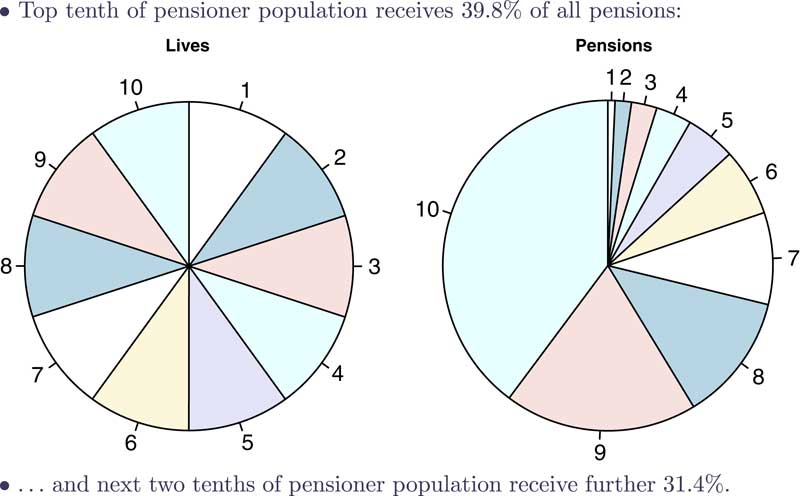
We will look again at the case study of the pension scheme in England and Wales. They were potentially interested in a buy-out or a longevity swap in respect of the pensions in payment only. They had a reasonable number of records. They had over 2,000 deaths in the data. They had about 16,000 lives once we had removed the duplicated benefit records. The further data is set out in Figure 1.
Top tenth of pensioner population receives 39.8% of all pensions and next two tenths of pensioner population receive further 31.4%

You can see how the portfolio looks. On the left you have the pensioners divided by lives into ten equally sized groups. On the right we sorted by the size of their pension. If we look at the weight of the liabilities we can see that some of these deciles of pensioners have almost no financial consequence whatsoever. Other deciles have a completely outsize impact on the portfolio. For example, the top 10% of lives are receiving 40% of all the pensions. If we look at the next two-tenths, we can see that they receive another 31%. So we have the situation here where 30% of the lives are basically receiving two-thirds of all the benefits. We have a completely disproportionate concentration of liabilities in a certain body of lives. This is particularly important for mis-estimation risk. We have this very simple model set out in Figure 2.
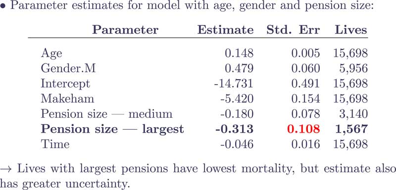
Parameter estimates for model with age, gender and pension size (lives with largest pensions have lowest mortality, but estimate also has greater uncertainty) Source: Richards (2014), Table 6
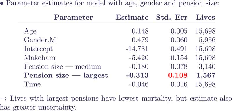
The group with the top 10% of lives gives a parameter estimate for pensions size – largest of −0.313. That means that these fairly wealthy individuals have markedly lower mortality than the people with smaller pensions. This parameter estimate comes with a higher standard error than a lot of the other parameters. Although this is an incredibly financially significant sub-group, with materially different mortality characteristics from the other sub-groups, this estimate of material difference comes with quite a lot of uncertainty on its own. This is why we want to look at the structure of the portfolio, because the lives with the greatest financial impact have the lowest mortality, but they also have some of the greatest uncertainty over just how much lower their mortality might be.
We asked the question: Why use a parametric statistical model? The answer is that the liabilities are concentrated in little sub-groups with different characteristics, and we use the parametric models to separate them and find what these separate characteristics are.
The other question was why we use a covariance matrix. The answer is that these parameters are not independent of each other but are correlated as set out in Figure 4 of the paper.
In this example, the same pension scheme data is adopted. The solid blue line is the best estimate. If we just consider the intercept and subtract two standard errors from the intercept and refit it, we find that the optimum age parameter increases because the rate of increase with ageing and the intercept are very strongly correlated. It is not just a question of simply shifting the mortality table down or up. We have to be aware that these things can pivot. Age is correlated not just with the intercept but also with other parameters that are correlated: for example, age and the effect of being male has 23% correlation. The parameter for being in the largest pension group and being male are negatively correlated.
There are a lot of positive and negative correlations between various parameters. This tells us why we need to use the whole covariance matrix. The covariance matrix tells us not just the uncertainty over the parameters, but also how the parameters are interrelated. We want to acknowledge these interrelations, which are shown in Figure 3 of the paper.
Model for survivorship – perturb it!
Uncertainty also varies by age, as demonstrated the uncertainty is at its least in the middle of the graph with the ages around age 80. Uncertainty is at its widest for the very youngest and the very oldest ages. We find that the mis-estimation capital varies quite strongly by age. It is relatively modest at the young ages. It gets progressively larger as the pensioners get older. This answers the question why we need to use a full portfolio valuation. The impact of mis-estimation varies by age and the various risk factor characteristics that the lives have.
The approach that I have adopted here allows for the concentration of risk. It allows for multiple risk factors. It allows for differing levels of uncertainty over these different risk factors. It specifically allows for correlations between the risk factors and the parameter estimates. It allows for the fact that the impact of uncertainty will vary by age. It allows for the liability profile of the portfolio.
In conclusion, mis-estimation risk arises fundamentally from having finite data or a limited amount of data. Mis-estimation risk is not something that you have to consider only for Solvency II reporting, it has a very direct application in pricing large transfers and large block deals like reinsurance. Any quantification that you make of mis-estimation risk should be financial and account for all of these correlations and the concentration of liabilities in these portfolios. As expected from any statistical exercise, the more data you have, the greater confidence you can have in your modelling parameter estimates. Consequently, larger portfolios will gain from having less uncertainty and thus a lower mis-estimation capital.
The Chairman: Thank you, Stephen (Dr Richards). The opener for the sessional meeting is Mr Kai Kaufold. He is the managing director of Ad Res, which is an actuarial consulting firm specialising in biometric risk analysis and reinsurance. He has worked recently on a list of projects including longevity swap reinsurance, basis risk, mortality improvements and experience analysis. Before founding Ad Res, he was responsible for Manulife’s European retrocession business. He qualified as a German actuary and holds a Master’s degree in physics from Cologne University. He has spoken at several conferences around Europe and North America.
Mr K. Kaufold (opening): As James (Crispin) said, my original academic background is in physics.
I have an international background, having worked in Germany and North America. Some of the companies for which I do consulting work are actually in the US and Canada. This will give you some context in which to set my remarks.
The reason that mis-estimation risk is something that is close to my heart is conditioning. When you go through university to become a physicist, they absolutely drum it into your head that there is no point in writing down a number if you cannot say how good it is. As a profession, it is very important that we are able to quantify how good our models and estimates are. If we cannot do that, then we cannot tell people how good our predictions are.
This is a very useful paper and I have found a couple of applications for it. Being able to quantify mis-estimation risk is one of the two main reasons why it makes sense to apply a statistical model to your experience to derive your mortality assumptions. First, as Stephen (Richards) mentioned in his presentation, you have the opportunity to understand the impact of the different risk factors that drive your mortality risk. So you are able to use statistics to find out more about your data than using traditional actuarial methods without statistics. You are also able to say how good your estimates are.
Whilst working for Manulife, I tried to use statistics in analysing experience and in projecting mortality. We had to use a brute force method to estimate parameter uncertainty. Instead of shaking the model the way Stephen described, we generated new sets of experience data using a statistical model. But we had to fit the whole model to that new experience data set. Thus you had to have a very tiresome process of estimating your parameter uncertainty. Stephen’s (Richards) method is much more efficient from a computing point of view.
Stephen also mentioned just a couple of practical applications apart from Solvency II. One application is pricing. As a reinsurer, I am not just interested in how much I am going to earn if I write a deal but also what is the likelihood that I am actually going to lose money. Leaders of reinsurers are usually more worried about the latter than the former.
In respect of valuation, I am going to show you an example of how in Germany we are trying to use mis-estimation risk to set valuation assumptions. Solvency II has already been mentioned in this context. I am also currently working on a project for the American Society of Actuaries to use a model that includes mis-estimation risk to help optimise how much reinsurance a company might buy.
The example relates to the additional reserve, or the reserve strengthening, that a company has to undergo because of the lower interest rate environment. The German life industry is allowed to use rolling averages for interest rates. Thus, we do not have to calculate our reserves using current market interest rates all of a sudden. But it also means that the pain of lower interest rates is going to stay with us a little bit longer as well. This reserve strengthening is very painful so the regulator has publicly stated that they will consider companies using their own portfolio-specific assumptions, so long as they prove that these are actually prudent. That is where being able to say how prudent they are becomes very valuable financially. The currently available literature on this topic goes back to 1994 when the German market was deregulated and companies started to use their own assumptions. There was a paper by H. Loebus that described how to quantify mis-estimation risk and came to the conclusion that it was roughly 20%.
It derives this by looking at the total claims in a year for life insurance, protection and endowment-type products, not for pensions. Unfortunately, the probability of getting the number of claims wrong and the uncertainty associated with the level of reserves, are only very indirectly linked. Given the assumptions and complex calculations involved, the 20% may not be very reliable, although everybody can remember such a round number. However, now we actually have a chance to figure out exactly what that number should be by using the method that Stephen (Richards) has suggested.
Another example is a project where again I am using a model that includes mis-estimation risk to calculate the economic margins for prudence that I have to hold relative to my best estimate, under what the Americans are calling principles-based reserves. The Americans are starting to want to use modern actuarial methods. The American life insurance market is a very large one and also uses reinsurance very heavily. It is going to have a very large impact on company balance sheets to understand what reinsurance does to their reserves under the principles-based reserving environment.
If you think about it very simply, reinsurance reduces the riskiness in your business, so you are purchasing reinsurance protection to reduce the risk. In this project I am trying to determine the extent that margins will narrow and how this is affected by different types of reinsurance.
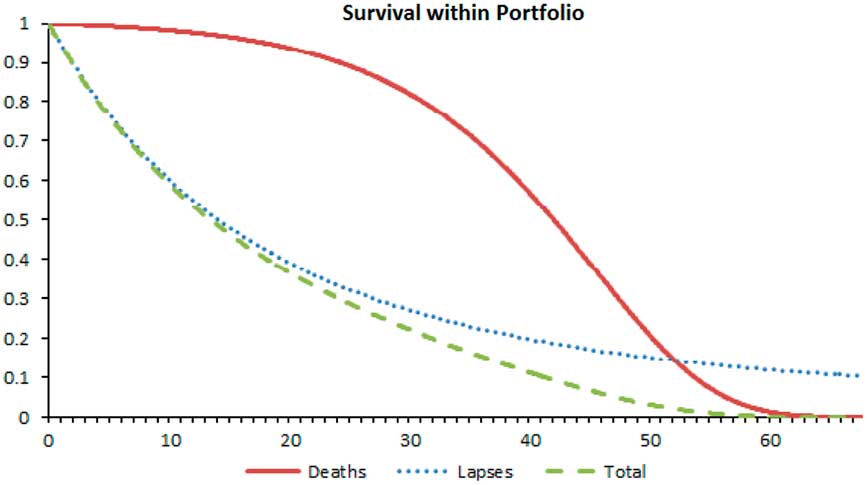
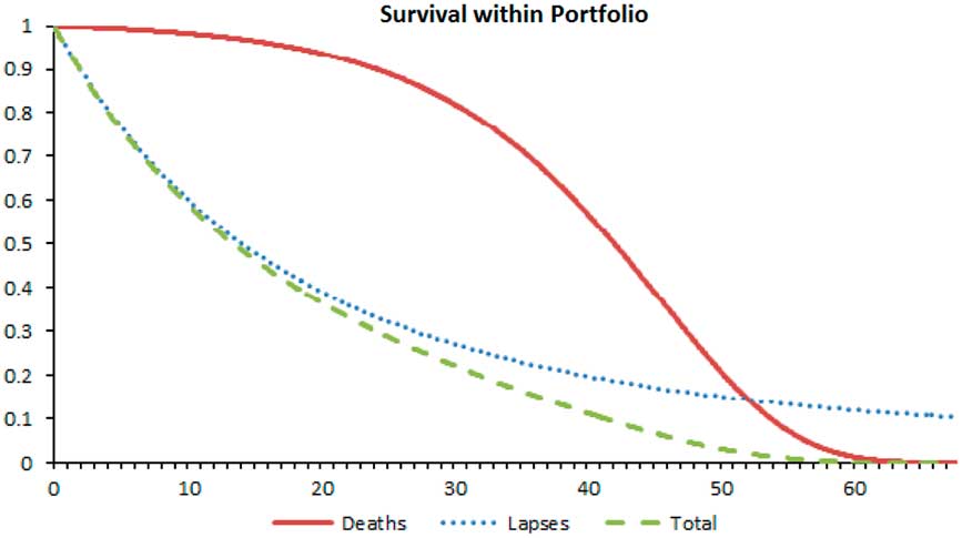
An important factor, apart from mis-estimation risk, is that you have even more concentration risk in a typical term life portfolio in the US than you would have in a pension scheme. The case study I am looking at is a 10-year term life product, and the largest policy is US$150 million. So if there is a claim on that policy, it is going to have a very big impact. I needed to model not just the uncertainty associated with my baseline assumptions, but each individual. I had essentially to do a projection using a model for each individual stochastically. This is very briefly how we did it. Using a survival model, we used a very simple Gompertz model and fitted it to the data. We found quite a number of different risk factors like policy size, smoker/non-smoker. The Americans have many underwriting classes but we found you can summarise them into three. We have a model that describes the mortality and survival of each individual and the lapse rate for each individual. Given this there is a certain probability of leaving the portfolio. That is the dashed green line (online only) that you can see on Figure 1.
I am interested only in the first little bit, but you cannot see very much so I left the whole survival curve on the chart.
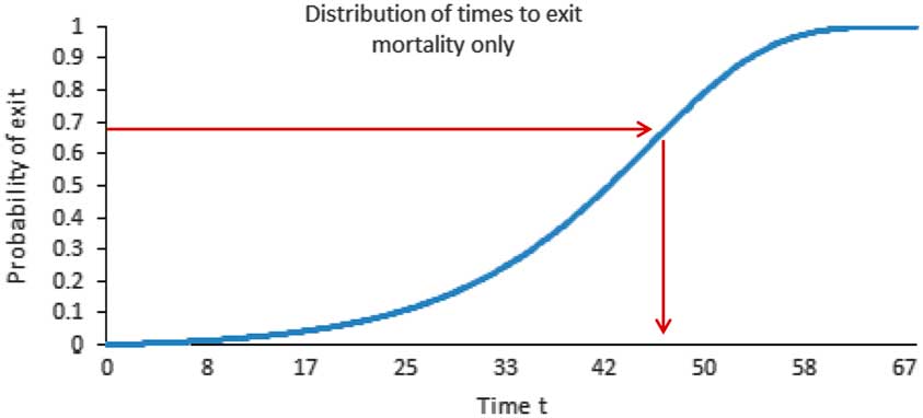
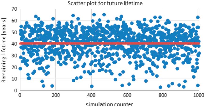
To carry out the mis-estimation risk calculation, as Stephen (Richards) explained, you perturb your model. Instead of generating new data you simply perturb your model and calculate your liabilities again. I do not want to calculate a best estimate for the liabilities under the perturbed situation. I am going to model each future lifetime for each individual and see what happens to the man with the US$150 million policy. All I have to do is pick a number between 0 and 1, uniformly distribute it and use the cumulative distribution of future lifetimes to figure out exactly how long that guy is going to live. The results are shown in Figure 4.
Random future lifetimes
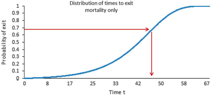
I do that a couple of times and I get a distribution of future lifetimes. If I know when they are going to die, then I know how much I am going to have to pay.
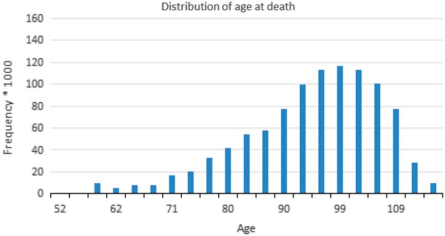
I am really interested in only the dots you can see on the Figure 5. The plot line also makes for an interesting picture; especially a little corollary: if you are always worrying only about your expected value, you are not getting the full picture. This was a 52-year-old male, non-smoker in a super-preferred class. He is going to live to a good age of 92 on average. But it is likely that he is going to become older than 92 because my distribution is skewed as shown in Figure 6. This is something that we have all seen but it is important to realise what those distributions actually mean financially.
Simulate individual lifetimes

Aggregate over N simulations

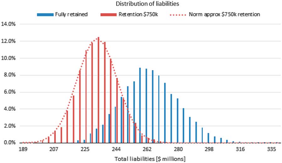
If I do the simulation for all of those individuals, I can calculate the total claims that I have to pay for these, and I can look at the total distribution of claims under the different perturbed scenarios.
I carried out two pieces of simulation. First, determining the mis-estimation risk, allowing for the fact that a finite data set is used and I have looked at the idiosyncratic risk of that particular portfolio and its size distribution.
That gives rise to the blue distribution of future claims as shown on Figure 7. It is centred around US$262 million and it is a fairly wide distribution based on the scale that I have picked. In this instance, I have used a very basic kind of reinsurance, surplus reinsurance, where everything above a certain limit of US$750 million goes to a reinsurer and the insurance company is responsible for everything up to $750 million.
Impact of reinsurance on liabilities

If the reinsurer is paying some of the claims the distribution shifts to the left. The total amount that the company has to pay is less. But of course the distribution also gets narrower because the reinsurer has now removed some of the risk. That means that the valuation assumptions can be closer to the mean than if the company retains all the risk itself.
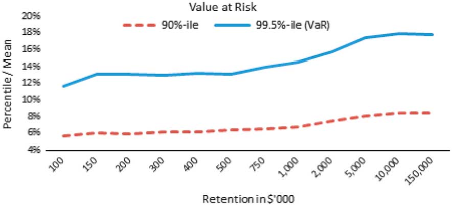
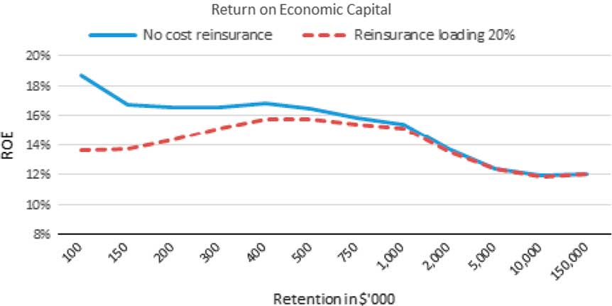
If I do that for a range of different retention levels, as shown on Figure 8 starting at fully retained, 150 is the largest policy; I have 99.50%, in the order of 80%, and you can manage to reduce that by lowering your retention and ceding more and more to the reinsurer.
Impact of reinsurance on liabilities – value at risk

The financial impact of reinsurance is of course that the amount of capital that the insurer has to hold is diminished. The question is whether reducing the amount of capital is worthwhile given the profits that the insurer is going to have to hand over to the reinsurer. So does it actually help the financial situation of the insurer to purchase reinsurance? The short answer is that it does, especially if the reinsurer is participating at exactly the same terms as the life insurance company. This is the blue line (online only) on Figure 9.
Impact of reinsurance on liabilities – return on economic capital

I have arbitrarily chosen the products to have a 12% return on capital if they are fully retained.
As you reduce your retention as the company cedes more and more risk, the return on equity or the return on that economic capital, increases. You have essentially to pick your threshold. For example, I need to make, say, a 16% return, so I need to purchase so much reinsurance. In real life, reinsurers do actually make money for taking on risk. Of course you are going to get an optimum because at some point it is going to be less efficient to buy more reinsurance. The optimum happens to be the 750 as shown on Figure 9. That is an actual example of applying mis-estimation risk to a non-pension and a non-annuity situation outside the UK.
This is a very useful paper. The technical application is very straightforward and it can be used for various different applications.
Mr I. J. Rogers, F.F.A.: How do you separate the mis-estimation risk from the model risk? It seems that it depends quite significantly on what model you use, and if you introduce more parameters to the model then there are more parameters that can be uncertain. You note in your paper that if you pick a model that is too simple, you materially understate the mis-estimation risk. So how do you know if you have chosen a model which is complex enough?
Dr Richards (responding): You are right. There is a tremendous risk of picking a model that is too simple and results in too low an allowance for mis-estimation risk. There is an example of this in the paper.
The way to deal with this is perhaps twofold. The first is applying a degree of judgement and common sense. So, for example, if you know that mortality rates tend to be changing over time, then you need to have an allowance for time trend in the model. In the pensioner case, mortality rates have been falling after allowing for other risk factors, so you have to have a time trend parameter in the model. If you have a time trend in your data set, for example, caused by falling mortality rates, it is remarkable how much of the benefit of having a larger scale data set from a longer period of observation will be undone and your mis-estimation risk will rise because of the uncertainty of just how strong the trend has been and thus the level of current mortality rates.
There is a second more mechanical aspect to determining whether your model is adequate. That is to do some kind of bootstrapping exercise where you sample a group of lives at random from your data set. You profile them according to your model and predict how many are going to die in the period observed. Then you compare the actual number of deaths with the number of deaths that are predicted by the model, and you do this both on a lives basis and weighted by some policy metrics, say sum assured or pension in payment. You are basically looking to make sure that this actual versus expected given the bootstrapping procedure is close to 100% on both a lives basis and an amounts basis. My experience is that for any reasonably sized data set, the lives-based actual over expected comparison is always very close to 100% on average for any model fitted using the method of maximum likelihood.
Whether or not your model includes enough of the important financially significant risk factors will be shown in the bootstrapping. You may find that a relatively simple model that includes, say, a tiered pension size or a policy size allowance, may often be all that is needed to get a bootstrapped ratio close to 100%, and that simple model may include age, gender, time trend and some policy metric. That is often enough to account for all the financially significant risk factors. You can add other risk factors that may not change the bootstrapping percentage but may actually provide a better fit. You may have smoker status or any other risk factor. It might not actually change the bootstrapping procedure but you may get some small changes in the allowance for mis-estimation risk, depending on how the concentrations work in the portfolio.
So in essence there are two approaches to answering your question about how to determine if you have the right sort of model. First, there is a substantial judgement element, making sure that the model is a broadly good fit, broadly sensible and includes things like time trends. Second, there is a more mechanistic approach where you use bootstrapping to check to see if you have captured most of the financially significant variation.
Mr R. R. Ainslie, F.F.A.: You mention in Paragraph 1.3 in the paper that you have come across a number of different methods currently used in practice that are used to quantify capital for mis-estimation risk. Using the method that you have described, do you think that other more ad hoc methods you talk about are tending to overstate or to understate the amount of capital that would be appropriate?
Dr Richards (responding): I could not really say. I have not seen enough of the mis-estimation capital allowances done in parallel. The mis-estimation procedure outlined here is used quite actively by a number of my clients. But I have never actually seen a side by side comparison of the old, ad hoc approach and with the results from the method presented here.
Mr Kaufhold (responding): In my analysis of the German reserves, I actually saw that the mis-estimation percentages were smaller than the paper from 1994 suggested.
Dr I. Currie: The title of the paper is “Mis-estimation risk: measurement and impact”. It is hardly surprising that you have concentrated almost exclusively on mis-estimation risk and its financial impact. I am disappointed that you made so little mention of model risk. These two things go hand in hand. It is hard for me to see that you can discuss mis-estimation risk without also discussing model risk. That occurred to me right at the very beginning of your talk when you covered the Gompertz mortality with its confidence interval. I do not know what you did there. I suspect that you fitted that model with a Poisson distribution. If you had, then you would have obtained very tight confidence intervals. My point is that very often the wrong specifications in the model can result in very tight confidence intervals. The mis-estimation risk would be grossly underestimated in that particular instance. In general I do applaud the concentration on mis-estimation risk but I would emphasise the importance of also taking into account model risk particularly for forecasting.
Dr Richards (responding): I did not entirely ignore the question of model risk in the paper. You are right that model risk is absolutely critical, perhaps even dominant, when forecasting. But this is not a paper about forecasting mortality risks, it is about the periodic estimation of mortality rates, and here model risk plays a very different role.
There are perhaps two ways of looking at model risk. One is the broad structure of your model assumption, for example, whether it a Gompertz or a Makin model and the distribution you assume for individual lifetimes, then there is the other question of what risk factors to include in the model. For example, whether to include pension size, smoker status, gender or the number of bounds, say, three or six.
Regarding the broad distributional structure you have for individual lifetimes, I tend to find there is not a very big difference between the different choices of models. If you actually switch from, say, Gompertz to Makin the impact on mis-estimation risk is actually really very small indeed. That is in stark contrast to projection models, where if you switch from, say, Lee-Carter to Cairns-Blake-Dowd (CBD) to P-spline, you will get some very different answers. That is why I regard model risk as perhaps the biggest and the most important risk facing you in forecasting. But switching between different model structures has a very modest impact on mis-estimation risk.
The other aspect of model risk is which risk factors to include in the model? That is covered in the paper although it is not specifically called model risk. I identified age, gender, time trend and pension size as the absolute minimum that you have to include to avoid another aspect of model risk, which would be too simple a model. This touches on perhaps the fundamental difference between the actuarial view of the world and the statistical view of the world. A statistician may approach a data set looking for any statistically significant risk factors. An actuary is interested in these but looks one step forwards to consider the impact of that risk factor. There are instances where statisticians choose to leave a parameter out of a model because it is not statistically significant. An actuary may choose to leave the parameter in the model because it has a financial impact.
A good example of this is the interaction of risk factors with age. We tend to find that any risk factor that gets fitted will also vary in its impact with age. Those individuals with large pensions have a very large mortality deficit at young ages, but it wears off as they get older and has by and large vanished by the time that they get to age 90–95. Often with portfolios you will fit these age interactions and there will not be enough evidence to justify keeping the parameter. From an actuarial perspective and experience you know that these risk factors vary with age and you also know that this has an important impact on liabilities. So while the statistician might say these parameters are not necessarily justified, the actuary would say they do have a rather important impact on the liabilities, therefore they should be included. So there is an element of actuarial judgement in the building of these models, which you could perhaps also include under the heading of model risk.
Prof A. J. G. Cairns, F.F.A.: In your last comments, you touched on the forecasting part of longevity risk in the paper for which you fitted a deterministic time trend. Obviously, there are other stochastic models. You mentioned Lee-Carter and CBD. In those models there is parameter estimation risk. Would you classify that under mis-estimation risk or would that fall under the other category that the PRA were mentioning as being the risk related to the trend in longevity improvements?
Dr Richards (responding): Different practitioners may have different views on this. I would classify that under the trend risk relating to future improvements.
In practice, a number of papers find that the uncertainty over the choice of model, or model risk, leads to as big a degree of uncertainty as you would get from the confidence intervals from a single model.
I would normally incorporate the parameter risk to which you are referring in the confidence intervals for a particular choice of forecast. So I would put it under the heading of future improvement risk.
Prof Cairns: I would stress that additional parameter uncertainty is extremely important, particularly where you have a portfolio of very long-term liabilities, such as pensions. With annuities in particular, that uncertainty in the trend parts is absolutely critical. In the case of term insurance, it might not be quite so important.
Mr Ainslie: I would be interested in your views on the interplay between basis risk and mis-estimation risk. In particular, of the case where you are designing a new product with new risk decrements and you are relying on population or other data for your early pricing, and at some point you might want to start introducing your own experience, even though you may be concerned about the credibility. Do you think that the mis-estimation risk techniques can help set capital for basis risk or minimum capital amounts for basis risk if you are using population rather than portfolio data?
Dr Richards (responding): The mis-estimation question presumes you actually have a sufficient body of clean, relevant data to work with. If you do not have any data in a portfolio, then you do not really have a mis-estimation problem. You do have a very major basis risk problem. I am not quite sure how different companies actually approach this issue. Some may just lump basis risk and mis-estimation risk together and deal with them using a single assumption. Other companies may choose to itemise them specifically.
Even if you have data, you need to ask yourself whether it is still relevant to the new business that you are writing. Until recently there was a very good example in the UK annuity market for individual annuities. Prior to 2000, there had been very little anti-selection, because there were not many enhanced annuities. If you had 5 years of mortality experience data for a relatively mature portfolio, you could analyse it and come up with estimates for the risk factors. You could also make a good estimate using this procedure as to what mis-estimation risk capital you would need to hold for your in-force policies.
Over the last 15 years, a lot of business has been written with a fair degree of anti-selection because of the growth of the enhanced annuity market. There is then the issue of whether the data that you have on your portfolio is wholly applicable. Any parameters that you might calculate, or models that you might fit to the data, may not be wholly applicable for all the new business that you have written over the last 5–10 years. There will be some important questions of actuarial judgement. It is not just a question of whether the data are clean but also whether there are enough of them. In addition, it is questionable as to whether the data are actually still relevant for all of the liabilities, especially the ones you have most recently written. In the case of entering a new market or writing a new product, it would be as much guesswork as anything else because the methodology here really does presume that you actually have data that is clean and relevant. I am not quite sure what I would do if I had to craft a basis with no experience data.
Mr H. R. D. Taylor, F.F.A.: First, the use of reinsurance seems to be able to reduce the amount of liability which is shown overall if it can reduce the mis-estimation risk. Are there any restrictions under the Solvency II rules around the use of reinsurance to optimise the reserves in a European insurer?
A follow-on question is that Kai (Kaufhold) specifically mentioned the impact of what I would describe as stop-loss reinsurance arrangements. I wondered whether the other type of quota share reinsurance had any impact at all on mis-estimation risk. In addition, in terms of innovation, are there any other shapes of reinsurance arrangement which could be derived between reinsurers and insurers which could be tailored specifically to reducing mis-estimation risk and therefore helping to reduce capital reserves that have to be held by primary insurers?
Mr Kaufhold (responding): Your first question was whether under Solvency II there are any restrictions on what kind of reinsurance a company might use to change their risk profile and change their capital. I do not know of any explicit restrictions. There are always restrictions in different national law. I know that there are restrictions in Germany around how much credit you can get for reinsurance under the German statutory valuation assumptions. That will have an impact on how useful it is in reducing your margins for uncertainty.
I am not familiar enough with your accounting rules here to comment authoritatively. That may seem a slightly vague answer. But the thing is with Solvency II the proof is in the pudding. You have to see whether you can actually convince your local regulator that you are reducing risk and that capital can then be commensurately reduced as well.
I probably should clarify the different reinsurance structures that I showed. I was referring to surplus reinsurance, which is a proportional reinsurance form similar to quota share. For quota share, the ceding company, the life company and the reinsurers share every risk in the same proportional percentage. For surplus reinsurance, which is also sometimes referred to as excess reinsurance, the reinsurer and the ceding company share every risk proportionately with the proportion depending on the amount of the risk. So it is a very simple, old-fashioned, type of reinsurance. I was just demonstrating that you actually get a reduction in your uncertainty from this type of reinsurance. When you do the same analysis for quota share, all you do is move the distribution to the left. But the width of the distribution stays exactly the same because you are not actually changing the risk profile. You are not making your portfolio more homogeneous to reduce your risk.
There are a number of innovators who are trying to introduce new forms of reinsurance to optimise Solvency II capital. There are only very few of them because most of the reinsurers are already very active in the market and are wary of cannibalising their own portfolios. At the moment in the UK market there is a tendency to reinsure literally everything, which is justified if you look at the chart that I showed. If you are the ceding company, if you assume that the reinsurer is not charging you extra for the additional risk that they are taking, that you are essentially sharing proportionately, then it makes sense to assume you get infinite return by not having any risk anymore because the reinsurer is essentially paying for it all.
Dr Richards (also responding): I believe, although I am not an expert in these matters, that the PRA has recently expressed unhappiness at insurers in the UK using reinsurance to optimise their Solvency II capital position. They basically expect to be approached before companies enter into any reinsurance agreements. So they are not at all keen on UK insurers using reinsurance to optimise their Solvency II capital.
The Chairman: I should like to thank everyone who has contributed. I will ask Stephen Makin to close the meeting. Stephen (Mr Makin) is a consulting life actuary and a partner at Hymans Robertson. He has a particular interest in the application of quantitative risk management techniques in insurance settings and advises clients on a range of matters including economic capital, quantitative and enterprise risk management, insurance restructuring, reinsurance and longevity.
Mr S. J. Makin, F.F.A. (closing): I enjoyed reading the paper. I found it to be very accessible, liked its structured approach and did not mind the maths, as well as finding it to be quite thought-provoking. I have one or two quibbles. They may not be important in the scheme of things but I am going to share them with you, nevertheless.
Solvency II does not prescribe that you must take account of mis-estimation risk. Although that is its effect, not least – and you pointed this out earlier – because the PRA have said that they consider mis-estimation risk to be a very important sub-component of longevity risk. That is quibble number one.
Ross (Ainslie), quite rightly, mentioned basis risk. It is not obvious that using portfolio data means that there is no basis risk. You, however, quite rightly, pointed to new to market and the selection effects and, effectively, the basis risk that that implies, so maybe I did not read the paper properly.
I would quibble also with the implication that a statistical model has to be used under Solvency II. The topic that we are talking about lends itself well to that, but I do not think that it is a general requirement. Expert judgement has a vital role to play. I think expert judgement is important not only in terms of interpreting the results, but also in and of itself. Although not explicitly the subject of the paper, it poses the question of how you can apply statistical techniques to quantify, for example, model risk? That is quite a tricky thing, whereas the statistical techniques you are talking about in the context of mis-estimation risk, are much more grounded and much more applicable and practical in my view.
The paper quite explicitly uses parameter risk synonymously with mis-estimation risk. My immediate questions were: Is that right? Does that even make sense? After a bit of puzzling, I concluded, as with so much in actuarial science, that the answer is, “That depends”.
If you assume that your model is correct then there is a risk that you mis-estimate the parameters from the data that you are using to fit the model. So if you are willing to start from that position, then parameter risk, using that synonymously with mis-estimation risk, is fine up to a point. But it does make the topic of model risk really important, because it fundamentally influences the risk of the parameterised model not being right.
So I conclude that parameter risk is an important part of mis-estimation risk, but as Ian Rogers quite rightly said, and Ian Currie underlined, certainly aspects of model risk are also extremely important. If you want the full picture, you do need to consider this. Model risk is absolutely fundamental. I agree also with Ian (Currie) on his philosophical point that there is a forecasting aspect to this and as such model risk is really important.
Generally speaking, economic capital requirements and economic capital frameworks require three things. They require a risk measure, that is, what are you going to use to quantify the risks against which you are holding capital? You need a probability level, that is, what is the level of significance or extremity against which you want to hold capital? They also need a time period, a time horizon. Over what time period are you considering the emergence of risks against which you are going to hold capital?
For Solvency II, the default calibration standard is a 1-in-200 1-year VaR. My main methodological comment on the paper is how the approach presented satisfies all of the calibration standards, of which there are three. The 99.5th percentile requirement is fine. The VaR requirement is fine. But I could not quite see how the 1-year requirement was dealt with. I would be interested to discuss this further.
In the context of trend risk, how to satisfy the 1-year part of the calibration standard has been the subject of a lot of debate in the industry over recent years. Stephen (Richards) has written a paper on this. Many firms have moved from what was a run-off approach to one that feels much more closely aligned to the default calibration standards.
In the context of mis-estimation risk, adhering to this 1-year part of the calibration standard is just as important. The number of years of data that you use to calibrate the model is potentially quite significant. I would urge at least some caution in using more than 1 year’s data. Just to be clear, I am not disputing that if mortality is a stationary process, static through time, then using many years of data will reduce parameter error in the sense that the maximum likelihood estimates have tighter error bands.
If your underlying model of the past is correct and you have all the historical mortality data that exists for the population, assume no basis risk, then there is no model risk and there ought to be very little parameter risk. However, if you are concerned with the uncertainty of mortality experience on an annuity portfolio, you do not necessarily get more certainty about the next year’s experience from looking at the past 10 years of data or 5 years or 3 years. Looking at it a bit more simplistically, analysing more data will not influence the uncertainty of experience over the next year. That is key to making this methodology appropriate in a Solvency II environment.
The calibration which includes the number of years data that you use is really important here. My own view is that you should start from a position of using 1 year’s worth of data and justify carefully, I am not saying that it is necessarily wrong to do so, why you would use more than this. It would need some thought.
What you would need to do before this approach, if to become anywhere near a Solvency II internal model, is go through a validation exercise. Tempting though it can be, validation is not just necessarily about saying why the chosen model is good. Rather, a good validation would start from understanding the model’s weaknesses with the ultimate aim of deciding whether or not the model is acceptable. Important questions are: What are the limitations of the model that you have chosen? And also what are the alternatives in terms of models and approaches?
In terms of limitations, you might wish to explore the validity of the information matrix approach as applied in the paper, that is an asymptotic approach. The question for me is what are the modelling limitations when applying that to a finite data set? That is something that at least needs to be explored.
On the subject of alternatives, as Ross (Ainslie) suggested, there are plenty of others. I am not sure that I would necessarily characterise them as ad hoc. I would just say that they are different.
One approach, either under some parametric modelling assumption or a bootstrapping technique along the lines that Kai (Kaufold) envisaged, might be to try to put some type of confidence interval around next year’s actual over expected ratio. This is not an uncommon approach. Then that resulting confidence interval could be used to guide the quantification of how extreme mortality might be over a year ahead.
Another approach which is consistent with the 1-year trend risk framework would be to fit a time series model to historical data and simulate outcomes over the next year and use that implied dispersion of future outcomes as a basis for modelling extremity over the year ahead. It introduces basis risk but it is another alternative.
Then with the final additional assumption that whatever it is you come up with is permanent, and it is a really important point which is often overlooked, you can then go about quantifying the impact of mis-estimations.
This is a thought-provoking paper and there is a lot to recommend it. There is a bit to be done perhaps before it immediately makes its way into anyone’s Solvency II internal models.
The Chairman: That brings us to the end of the discussion. Thank you everyone who participated in the discussion. I should also like to thank Stephen (Richards) for the paper. He has given us something to take away and think about when we look at similar problems in our own work. Also, thanks to Kai (Kaufold) for his contribution.