


The coherence of linguistic varieties has been increasingly questioned in recent years, for example in studies on ethnolects (Boyd & Fraurud, Reference Boyd, Fraurud, Auer and Schmidt2010; Wolfram, Reference Wolfram2007), dialects (Gregersen & Pharao, Reference Gregersen and Pharao2016), sociolects (Guy, Reference Guy2013), and registers (Geeraerts, Reference Geeraerts, Boye and Engberg-Pedersen2010). Results indicate that the lects labeled by linguists and laymen seem not to be realized in actual language use, and they should thus be reconsidered. The issue of lectal coherence (Guy, Reference Guy2013) has been examined by focusing on patterns of covariation instead of singular variables (e.g., Gross, Reference Gross2018; Oushiro, Reference Oushiro2016).
The sociolinguistic research on covariation patterns was introduced in Labov's study of English in New York City (Labov, Reference Labov1966:209–11). The study presented two approaches to stratification of linguistic data: social grouping and linguistic grouping. Social grouping (the assignment of speakers to sociologically defined groups) gained considerable popularity in the field after Labov's initial study, whereas linguistic grouping (search for patterns of linguistic behavior) has surfaced more rarely until recently (e.g., Horvath & Sankoff, Reference Horvath and Sankoff1987; Ma & Herasimchuk, Reference Ma, Herasimchuk and Fishman1972; Thelander, Reference Thelander1979).
Social grouping does not scrutinize linguistic systems per se but seeks to distinguish how (perceived) social systems affect linguistic features. If multiple features seem to behave uniformly in regard to social factors, the collection of these forms is considered a variety or a lect—a linguistic system under certain circumstances. Therefore, the varieties discovered in studies built on social grouping (i.e., sociolects) are reified by social factors such as class (“middle class speech”), ethnicity (“African-American English”), or locale (“Rinkeby Swedish”). This sort of essentialist approach has several problems that have been discussed at length (e.g., Bucholtz, Reference Bucholtz2003; Pratt, Reference Pratt, Fabb, Attridge, Durant and MacCabe1987).
Linguistic grouping starts from language use and searches for patterns of covariation. The issue with linguistic grouping is that the discovered patterns are often difficult to interpret. For instance, Ma and Herasimchuk (Reference Ma, Herasimchuk and Fishman1972:271) discarded four of ten patterns found in their study in part because “co-occurring items made little linguistic or sociolinguistic ‘sense’ as a unity.” The discovery, although disregarded in the study, is of utmost importance. The items were found to co-occur, but not in a way the researchers expected: the lects were not distinct and identifiable but rather obscure and overlapping.
The article at hand contributes to the field of lectal coherence by searching for lects of Finnish spoken in Helsinki. Based on real time interview data from the 1970s to the 2010s, we examine how phonological, morphological, and lexical features covary and thus constitute lects in Helsinki. We define a lect as a pattern of several frequently co-occurring linguistic features. This definition is entirely usage-based and does not require social similarity of the speakers (cf., sociolect). Whereas many of the studies mentioned focus on a small number of features (e.g., Guy, Reference Guy2013; Oushiro, Reference Oushiro2016), we scrutinize thirty-four linguistic alternation variables with seventy-eight possible variants. We do not restrict to mutually exclusive patterns; each variant can appear in several lects, and each speaker can exhibit features of multiple lects in their speech. To uncover the lects, a probabilistic component model called Latent Dirichlet Allocation (Blei, Ng, & Jordan, Reference Blei, Ng and Jordan2003) is used. The present article addresses the following questions:
1. Which linguistic variants covary and thus constitute the lects?
2. Can the discovered lects be traced to previously proposed lects of Finnish spoken in Helsinki, such as the standard language, the Häme dialect or the Helsinki slang (Paunonen, Reference Paunonen and Nordberg1994)?
3. Are the speakers likely to use single lects or combine them? And if so, which lects combine?
The growing body of work on lectal coherence suggests that the covariation among features is likely to be weak (cf., Guy, Reference Guy2013), and that there will be overlap and uncertainty between the lects (cf., Ma & Herasimchuk, Reference Ma, Herasimchuk and Fishman1972). Thus, we expect that, although we might discover lects that can be traceable to previously proposed lects of Finnish spoken in Helsinki, they will not be easily identifiable. Similarly, we expect idiolects to be combinations of several underlying lects (cf., Geeraerts, Reference Geeraerts, Boye and Engberg-Pedersen2010).
We commence with a brief history of the linguistic landscape of Helsinki, which clarifies why the Finnish capital is of particular interest when studying lectal coherence. We then introduce our data and the model used in more detail, before proceeding on to the results.
HELSINKI AS A LINGUISTIC MOSAIC
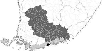
Helsinki was founded in 1550 but remained a minor town until the late eighteenth century. Sweden lost the territories of Finland to Russia in the Finnish war, and the new Russian regime moved the capital from Turku to Helsinki in 1812. At the time, the population of Helsinki was approximately 4,000 and almost entirely Swedish speaking (Paunonen, Reference Paunonen and Nordberg1994; Waris, Reference Waris1951). Considering that the study at hand scrutinizes Finnish varieties, this is highly important. As the settlement's history is relatively short and the population was mostly Swedish speaking, the city lacks a Finnish dialect basis. The linguistic situation of the early twentieth century is illustrated in Figure 1.
Map of southern Finland. Present-day Helsinki in black, Swedish-speaking areas in light gray and the areas of the Häme dialect in dark gray (based on Itkonen, Reference Itkonen1989). The map represents the linguistic situation in the early twentieth century.

The capital status and industrialization rapidly increased the number of residents and spurred migration from Finnish speaking areas. The migrants were mostly from neighboring regions Uusimaa and Häme. The Finnish variety spoken for the most part in these areas was the Häme dialect, that is of interest also in this study (dark gray in Figure 1). The dialect itself is divided into several subdialects (Itkonen, Reference Itkonen1989) from which the Southern Häme dialect is of particular interest in our study. Although there was migration from the Eastern parts of Finland as well, the features of the Eastern dialects never gained much popularity in Helsinki (Paunonen, Reference Paunonen, Juusela and Nisula2006). The language situation changed speedily: from ten percent Finnish speaking residents in 1850 to 45.5 percent in 1890 (Åström, Reference Åström1956). In the beginning of the twentieth century, Finnish was already the majority language in Helsinki.
In the wake of the nineteenth century nationalist movement, several members of the Swedish-speaking elite decided to start speaking Finnish between each other and in their homes (Paunonen, Reference Paunonen and Nordberg1994:229). As stated earlier, there was no base dialect of Finnish in Helsinki to learn, which led the elite to speak a standardized version of the language. The Finnish standard language is an artificial creation that combines features of the Western and Eastern dialects and is thus not based on any single natural dialect (Lehikoinen & Kiuru, Reference Lehikoinen and Kiuru1989). It is also relatively new, as the standardization was executed as late as the nineteenth century. The standard language as a spoken variety is highly salient, as it is distinct from all the dialects. We argue that we are almost certain to discover a lect traceable to standardized Finnish in the results of this study.
In working-class suburbs, Finnish and Swedish co-existed, generating the old Helsinki slang around the turn of the twentieth century. The slang combined Swedish, Finnish, and Russian lexis, utilized Swedish phonemes (e.g., /b/), and was spoken by those of Finnish- and Swedish-speaking descent (Paunonen, Reference Paunonen and Nordberg1994). The old Helsinki slang has faded since the Second World War, and the new Helsinki vernacular is generally Finnish-based, with new loan words coming mostly from English.
The amount of people speaking languages other than Finnish or Swedish as their native language has risen rapidly in the last thirty years in Helsinki. In 1990 only 1.3% of residents were speakers of other languages, whereas, in 2019, the proportion was 15.7% (Mäki & Vuori, Reference Mäki and Vuori2019). Unfortunately, individuals whose first language is other than Finnish cannot be reached in the study at hand, as the data is exclusive to native Finnish speakers. The increase of other languages is bound to affect the lects of Finnish spoken in Helsinki in the future (cf., Gross, Boyd, Leinonen, & Walker, Reference Gross, Boyd, Leinonen and Walker2016).
Helsinki has seen several language and dialect contacts in the past two hundred years: between Swedish and Finnish and Russian, between Finnish dialects, between dialects and the standard language, and between the increasing number of new languages in recent decades. Mufwene (Reference Mufwene2001:4–6) described such a situation as producing a feature pool from which new varieties are constructed and modified (cf., Cheshire, Kerswill, Fox, & Torgersen, Reference Cheshire, Kerswill, Fox and Torgersen2011). The old Helsinki slang is an example of an output variety that was composed of features of the pool selectively and constituted a unique combination of the input varieties.
In a similar vein, but discussing stylistic practices, Eckert (Reference Eckert2008) described the process of bricolage (see also Hebdige, Reference Hebdige1979). In bricolage, linguistic variables (and other social resources) are distinct features of a style. Once a feature is perceived, the observer can choose whether or not to use it in their own speech. The use of a feature in a new setting changes both the meaning of the feature and the originally perceived style. Thus, bricolage might disrupt the coherence of lects as a speaker decides to use a feature not originally belonging to a certain lect, or speakers may condense the lects into even more coherent bundles as they accommodate to lectal norms in their selections. For a contrastive study of a variety approach and a stylistic approach to lects, see Quist (Reference Quist2008).
To conclude, the input varieties of Helsinki Finnish can be simplified to three separate lines: the highly standardized Finnish introduced by the elite, the rural dialects (especially Häme) of the migrants and the slang of the working-class neighborhoods. Residents of the capital area themselves define the lects spoken in Helsinki mostly in relation to the old slang or the standard language, using characterizations such as “modern Helsinki slang,” “neither book language nor slang,” and “standard with a few slang words” (Vaattovaara & Soininen-Stojanov, Reference Vaattovaara, Soininen-Stojanov, Juusela and Nisula2006). In the same study, most cited features of Helsinki Finnish are slang words, fast tempo, and the Helsinki -s (see Halonen & Vaattovaara, Reference Halonen and Vaattovaara2017). Thus, the dialectal features, which, in reality, form the basis of the spoken language in the area (Paunonen, Reference Paunonen1995) are not perceived or identified by the speakers.
DATA AND METHODS
Longitudinal Corpus of Finnish Spoken in Helsinki
The data analyzed in this article is a subset of the Longitudinal Corpus of Finnish Spoken in Helsinki (Helpuhe). The corpus project started in the beginning of the 1970s as a part of a sociolinguistic enterprise to study the spoken language of Finland's biggest cities. In the guidelines of the sociolinguistic studies of the time, the method was to conduct interviews of the city's native residents with varying social backgrounds. The original endeavor involved three age groups, three social classes, two socially different districts, and two genders. The neighborhoods chosen in the original study were academically inclined Töölö and a working-class district Kallio-Sörnäinen, which was also the birthplace of the old Helsinki slang (Paunonen, Reference Paunonen, Juusela and Nisula2006). In total, 149 speakers were interviewed between 1972–1974, from which a corpus of ninety-six speakers was created.
The project continued in 1991–1992, when the two youngest age groups of the 1970s study were pursued again. Nearly half of them were interviewed again (29/64), supplemented with a new group of youngsters. In total, the number of interviewees is significantly lower in the 1990s subset than in the 1970s (forty-five and ninety-six respectively). The youngest group was chosen using the same guidelines as in the 1970s, but the distinction between three social classes was simplified to present high schoolers and vocational school attendees. Moreover, the demographic conditions of the Kallio-Sörnäinen district had changed in the twenty years between the interviews, and it did not represent a working-class neighborhood anymore; thus, the district restrictions were loosened. The third cycle of the project was carried out in 2013 in a similar fashion. A good proportion of the interviewees in the last cycle was reached (27/45) and augmented again with a new group of adolescents, divided equally in high school and vocational school. All in all, thirteen speakers have been interviewed in all three time points.
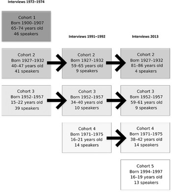
Three age groups were studied in all three decades. These represent young speakers, middle-aged speakers, and old speakers, but vary in the actual ages of the interviewees. In the 2010s subset there is also an additional group of four 81- to 86-year-old informants. The ages, birth years, and number of speakers in each group is presented with the temporal structure of the data in Figure 2. The corpus is a combination of panel and trend data, as the 1990s and 2010s subcorpora consist of middle-aged and old speakers already interviewed in earlier stages, bolstered with the young group. This leads to imbalance in scale, as the 1970s subset is much larger than the following ones. The data analyzed here consists of 126, thirty-three, and forty informants in the 1970s, 1990s, and 2010s, respectively. The panel data also tends to emphasize the academic speakers, as it has been harder to reach the speakers of lower social classes (Paunonen, Reference Paunonen, Juusela and Nisula2006; cf., Sankoff, Reference Sankoff, Wagner and Buchstaller2018).
Structure of the data (based on Paunonen, Reference Paunonen, Juusela and Nisula2006). Time of the interviews is presented along the x-axis, and the cohorts are visualized in shades of gray. The number of speakers in each cohort is reported in the rectangles along with the ages at the time of the interview.

Through all three time points, the interviews were conducted by the University of Helsinki students. A recurrent pattern of questions was provided for the interviews in every cycle, but it has not been followed equivalently in every interview. The questions were about the informants’ and their families’ lives, traditions, and perceptions of Helsinki and the Helsinki Finnish, as well as other dialects and languages. Every interview lasted for about an hour, and at least thirty minutes of every interview has been transcribed. The transcribed excerpts are not consistent (e.g., first thirty minutes) but vary between the interviews. It has been noted that some speakers in the 1970s regarded the interviews as formal situations (Paunonen, Reference Paunonen2005:186), and such attitudes were not present in the 1990s or 2010s. This might affect some of the changes we observe.
Analyzed features
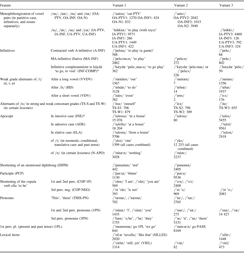
The features analyzed in this study are mostly based on previous studies of Helsinki Finnish (e.g., Paunonen, Reference Paunonen1995, Reference Paunonen, Juusela and Nisula2006). In addition, some features were chosen because of their prevalence in a pilot study. The features are mostly morphophonological, but some syntactic and lexical items are studied as well. We present the analyzed linguistic features and their respective variants in Table 1. Each feature is given a short name to refer to in the text. The frequency of each variant is also presented in the table. To give the reader an understanding of the variants and their relations to previously proposed lects, we give a brief explanation. However, we do not test if the previously proposed lects occur in the study (a hypothesis model); instead, our exploratory model finds collections of variants that best explain the variance in the data. For an international audience however, some backdrop is needed.
Studied features. Variant 1 represents pronunciation in standard Finnish and Variant 2 in the Häme dialect. Variant 3 represents variants from several differing origins, most of which can be associated with Southern Häme

The first variants in Table 1 represent the pronunciation of the feature in standard Finnish. The standard is a combination of Western and Eastern dialect features, which leads the standard and the Häme dialect, for instance, to coincide in some cases. Using the standard variant, therefore, does not always represent deviation from dialectal features. Some standard variants have a social index (Silverstein, Reference Silverstein2003), however. Using the first-person plural form /’menemme/ (1PL1) for instance comes across as very formal.
The differing social meanings present problems for the idea of coherent lects. Consider a case in which a speaker uses a single standard language variant that comes across as highly formal amid other varying features. Another speaker consistently uses several standard language features that are not as salient markers. The one variant can provoke a second-order indexical link (Eckert, Reference Eckert2008; Silverstein, Reference Silverstein2003), whereas the use of several first-order features might not be noticeable to laymen. Thus, the first speaker might be perceived as more correct and formal (to use folk linguistic terms), although in the light of lectal coherence this would not be the case. Earlier studies (e.g., Campbell-Kibler, Reference Campbell-Kibler2011; Johnstone & Kiesling, Reference Johnstone and Kiesling2008) have reported on how a single variant affects perceptions on matters such as intelligence of the speaker, formality of the situation, or locality. A similar perception study on lects would shed light on ways in which laymen label different ways of speaking.
Continuing with Table 1, the second variants represent the use of the variable in the Häme dialect. This is not the case in the variables INF-COMP and INE (marked with asterisk) however, in which the first variant is used in the Häme dialect. In these two cases, the second variant represents the feature in other Western dialects. In all the cases where the second variant is empty, the Häme dialect coincides with the standard. In some cases, the second variant is not exclusive to the Häme dialect but more generally used in Finnish dialects (e.g., DIPH, PCP, COP, 3PN, 1PL). The last column (Variant 3) collects variants of differing origins: for instance, from Southern Häme, which differs slightly from the main Häme dialect (A-INF), Eastern dialects (HD), and widespread vernacular features (1PN).
Before continuing to the method of the study, a word of caution is presented. The interviewees of the corpus are native speakers of Finnish born in Helsinki. Although some of them have since moved or lived elsewhere in between the interviews, the corpus is designed to be quite homogenic, continuing the traditions of dialectology. This of course influences the variance we encounter and the different lects the method is able to discover. Ethnolects, for instance, are not analyzable with the corpus at hand.
The features selected for the study also need to be scrutinized. Most features are morphophonological, only few lexical, and none prosodic. It has been stated that the surface of the language (i.e., lexical and phonetic features) shows greater social stratification than grammatical features (Meyerhoff & Walker, Reference Meyerhoff and Walker2013). However, Levon and Buchstaller (Reference Levon and Buchstaller2015) found this does not hold for listener perceptions: listeners attended a morphosyntactic variant differently than a phonetic one, but it was subject to evaluation nonetheless. Even in production studies, results are conflicting (e.g., Cheshire, Kerswill, & Williams, Reference Cheshire, Kerswill, Williams, Auer, Hinskens and Kerswill2005). We believe emphasis on the morphophonological domain in our study does not compromise the results. It must also be noted that Finnish is an agglutinative language, and results of studies on English are not therefore directly applicable.
Latent Dirichlet Allocation
The aim of the current study is to discover which variants co-occur in the data and thus create a linguistic pattern, a lect. Several methods for identifying covariation have been used in sociolinguistic settings before, such as factor analysis (Spearman, Reference Spearman1904), principal component analysis (Pearson, Reference Pearson1901), and k-means clustering (Forgy, Reference Forgy1965). In the study at hand, a Latent Dirichlet Allocation (LDA) model is used (Blei et al., Reference Blei, Ng and Jordan2003).
LDA is a probabilistic model of the occurrence of countable features in each document. Typically, these countable features are the number of occurrences of different words, but, in our work, they are the number of occurrences of the different linguistic variants listed in Table 1. In LDA, these counts in each document are assumed to arise from a mixture of underlying components. In machine-learning literature, these components have traditionally been called topics. We abstain from using this term, as we do not search for topics in a linguistic sense. We use the term component when looking at the data at the level of the computational model and lect when looking at the linguistic interpretation of the computational analysis.
Each of the components k = 1,…,K has a probability distribution over the features v = 1,…,V, denoted as p(v | k), and each document d has a probability distribution (mixture) over the components, denoted as p(k | d). The probability for a particular feature to occur in the document is then a sum over the components, p(v | d) = Σk=1,…,K p(v | k) p(k | d). The contents of each distribution p(v | k) and each distribution p(k | d) are found by fitting (optimizing) the model for the observed data, according to what best describes it. In practice, features that often co-occur will form one of the components and have high probabilities within it, but the same feature can also become associated with multiple components if, for example, it co-occurs with one group of features in one context and with another group in another context.
The decision to use LDA for our corpus of spoken Finnish is based on an analogy. LDA has already been used in text classification and considers documents and words. Based on the co-occurrence of words in the documents, LDA infers hidden topics for the corpus. For instance, if the words dog, bone, and fetch appear in several documents together, whereas cat, meow, and kitten appear in others, the model infers that these two collections of words represent different topics (dogs and cats, although the model does not know the labels). If we understand lects as collections of frequently co-occurring linguistic features, the analogy is simple enough. The interview transcriptions we use correspond to the text documents, and the linguistic features we have picked correspond to the words in the documents. Instead of finding latent topics as in text classification, we attempt to find underlying lects: if the features 1PL1, INE1, and ADE1 co-occur in several interviews, the model starts to infer that they represent a lect. However, the model does not restrict the number of co-occurring variables that can define a component, which means that it could also discover collections of only a few features. In these cases, we must use linguistic reasoning to decide which components represent lects. This is another reason to use the term component when discussing the results of the model.
Although the analogy is for the most part simple, there are some differences between these two data types. First, when the model is used for text documents, all the words (apart from very common words such as and) are used to fit the model. In our data, we have focused on a chosen set of linguistic features and collected them from the interviews. Thus, our decisions already force the model in a certain direction. Another important difference is the fact that text corpora are generally sparse. This means that the words might appear frequently in some documents but not at all in others; in terms of matrices, there are a lot of zeroes. There is not a lot of sports vocabulary in articles about quantum physics, and vice versa. This is not the case in our data. We have only seventy-eight possible variants in our data, several of which appear in most of the interviews.
One of the benefits of using LDA instead of other clustering methods like k-means is the fact that it is a mixed-membership model. This means that each of the variants under study can be a part of any component, and each interview can be a mixture of unlimited components. It therefore supports a fluid understanding of language use, as the variants and components can be combined in an unrestricted manner. This is an important attribute: if a computational model is asked to do strict categorization, the results may appear more coherent than the linguistic reality is.
The variants were searched for in interview transcriptions using regular expressions (Thompson, Reference Thompson1968). The search results were manually verified and collected to a data frame automatically, using the statistical software R (R Core Team, 2017). The LDA model was then run on the resulting data frame using the R package topicmodels (Grün & Hornik, Reference Grün and Hornik2011).
RESULTS
We set out to examine which features covary in Finnish spoken in Helsinki and whether the discovered components were intelligible and interpretable in terms of previously proposed lects. We hypothesized that there was likely to be weak covariation of features in the data and that, although we might discover components traceable to different historical processes, we would also find plenty of obscurity in the data.
We begin by fitting the model to find the statistically most coherent components. After this initial stage, we start analyzing the components in regard to their distinctiveness, which is defined as the variants’ exclusiveness to components. In this section, we will also comment on the components that can be traced to previously proposed lects. To take a closer look at the lects and their utilization, we examine the primary components in the interviews and scrutinize the volume in which they are used. We furthermore analyze which components are likely to combine in use. Finally, we take a short look at the variation and change of the lects in real time. Based on these analyses of the inferred components, we define the linguistically realistic lects and their divergence from the mathematical components.
Coherence and distinctiveness
When using the LDA model, the number of components must be defined beforehand. There are several mathematical methods to find the best fit. In this study, we used two separate tests (Cao, Xia, Li, Zhang, & Tang, Reference Cao, Xia, Li, Zhang and Tang2008; Deveaud, Sanjuan, & Bellot, Reference Deveaud, Sanjuan and Bellot2014). We performed a hundred iterations of model training for each fit, where the number of components ranged from two to fifteen. Both tests found a model with ten components to present the best fit and thus the most coherent components. We further checked the three best models of each of the preceding tests for the Akaike Information Criterion (Akaike, Reference Akaike1974) and Bayesian Information Criterion (Schwarz, Reference Schwarz1978) values. These values also signaled that the model with ten components presented the best fit for the data. We thus ran the model for the whole dataset with ten components. We ran the model for the three decades’ (1970s, 1990s, 2010s) separately as well and compared the results with the whole data set. The division to three subsets did not significantly alter the discovered components, which led us to focus on the complete set in the analysis.
The LDA model returns two objects: probabilities for variants per component and probabilities for components per interview speech. The probability of a variant's appearance in a component emphasizes the frequency of the variants in the data and not their exclusiveness to one component. Some variants appear in an interview hundreds of times, whereas others occur only a few times (see Table 1). This is problematic for linguistic interpretation, as the components are often headlined by the same features. To counter the issue and discover which variants are mostly associated with which components, we calculated conditional probabilities using Bayes’ theorem (Bayes & Price, Reference Bayes and Price1763): (P(Componentk|Variantv), probability of Componentk given Variantv). This process brings the variants on the same scale: because there are ten components and the probabilities always sum to one, the average probability per component (given a variant) is 0.1. Thus, conditional probabilities above 0.1 index a higher association with a component than in average. If a Componentk has a conditional probability of one given Variantv, all utterances of Variantv are associated with Componentk.
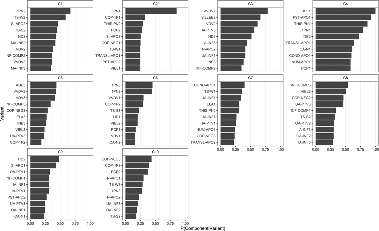
We scrutinize the variants that produce highest conditional probabilities in the components in Figure 3. We use the feature labels presented in Table 1, followed by the number of the variant. For instance, 3PN2 represents the second variant of the third person pronoun variable. In the figure, the complete probability scale is shown. The more exclusive the variants are to the component in question, the longer the bars. We want to emphasize that exclusiveness to a component does not necessarily indicate that the variant is highly important to it: for example, if a variant appears only seven times in the whole corpus, it does not carry much weight in the fitted model, but might still be (and most likely is) highly exclusive to a single component. Thus, the conditional probabilities shown in Figure 3 might emphasize variants that are very rare in the corpus. These cases are commented on when necessary. The probabilities of variants per components (which in turn emphasize very frequent variants) are presented as the supplementary Figure S1 in the Appendix.
Highest conditional probabilities of components given variants. Components are labeled as abbreviations (C1 = Component 1). The variants are labeled as in Table 1.

The first observation of the figure is that C2 is headlined by a single variant. C6 is also unevenly distributed. C5, C7, C8, C9, and C10 are more coherent internally, but the probabilities are not high, which indicates that these components consist of features frequently used in other components as well. Finally, the three components that appear to be the most distinct are C1, C3, and C4. We will begin by analyzing these three components before moving on to the more uneven ones.
C4 appears to be the most distinct of the discovered patterns, as some variants are almost exclusive to it. The ten highest ranking variants instantly reveal the nature of this component, as they are almost entirely from standard Finnish. The only exception is INE2, an infrequent variant originally from the Western dialects. The variant producing the highest conditional probability (1PL1) was discussed earlier in regard to second order indexicality. It is completely exclusive to C4. Other variants in C4 are also quite distinct and index formality or correctness: the preservation of the word-final /i/ in PST-APO1, TRANSL-APO1, and NUM-APO1, as well as the use of standard language pronouns /’minæ/ ‘I’, /'sinæ/ ‘you’ (1PN1), and /’tæmæ/ ‘this’ (THIS-PN1) are all relatively rare in Helsinki (Paunonen, Reference Paunonen1995). Thus, our hypothesis of discovering a standard Finnish variety in the corpus is realized in C4. It is, in fact, not a surprise that this lect is the most distinct of all, given its enregistered nature (Agha, Reference Agha2003). Similarly to RP in Agha's study, standard Finnish is also a variety whose correctness is guaranteed by someone else. Hence, there are clearer rules to follow to use this lect. This opens possibilities for ideological work: a speaker may refer to the variants in standard Finnish to sound upper class or more educated.
Unlike C4, C1 and C3 do not have any standard Finnish variants among their most distinct ones. Both have several variants of the Häme dialect, but C3 has more features associated with Southern Häme, which is situated closer to the capital region. IA-PTV3, A-INF3, and INE3 are all common in the Helsinki region, but not in the heartlands of Häme. Interestingly, though, C1 uses zero as the alternative to standard Finnish /d/ (HD3, VVDV3), which is a variant originating in the Eastern dialects but very common in spoken Finnish all over the country at present. The alternative to standard /d/ in C3 is /r/ (VVDV2, VDV2, HD2), historically used in the Western dialects (including Häme) but quite rare in contemporary Finnish. It is also very rare in the data at hand, which means that it cannot be given too much weight in the analysis. Concluding from these differences between the two components, C1 can be traced to the Häme dialect, whereas C3 can be traced to Southern Häme.
These three components are thus interpretable in terms of previously proposed lects and can be labeled accordingly to ease reading of the article. We shall call C4 the enregistered standard (cf., RP in Agha, Reference Agha2003), C1 the Häme dialect, and C3 the Southern Häme dialect. To reflect on our hypotheses, the results are quite surprising. The three most distinct components are easily traceable to previously proposed lects. Thus, the coherence of these lects is also visible in the data at hand. Especially the enregistered standard (C4) shows significant coherence and distinctiveness. However, we need to take a further look at the seven remaining components before making overall interpretations of our results.
C6 and C10 share features, as there are both 1PN (first and second person pronouns) and COP-1P (first and second person present tense of the verb olla ‘to be’) variants among them. They are thus constituted by phrases such as /’mæ ‘oon/ ‘I am,’ which are naturally quite likely to occur in interview speech. Both components are mostly focused on these two variables. C6 hardly gets even a 0.25 conditional probability for any other variant. Moreover, in C10, the highest conditional probability belongs to the negation of the copula (COP-NEG3 /’ei ‘oo/) which also appears with the first and second person pronouns. As there are no restrictions on the number of variants needed to compile a component, only a few frequently co-occurring linguistic items suffice. Such a possibility was discussed in the previous section, and these two components demonstrate it in practice. Thus, although components 6 and 10 are collections of co-occurring features, they must be interpreted as repeating phrases rather than lects.
C2 is similar to C6 and C10, as the conditional probability given 3PN1 (/’hæn/ ‘s/he’) is 0.85 and the next highest probability is 0.33 (COP-1P1). This might indicate that the third person pronoun appears in multiple contexts and is not tied to any of the other components. The variant is discursive in nature and interpreted as age-graded (Lappalainen, Reference Lappalainen, Lappalainen, Sorjonen and Vilkuna2010), which could explain its somewhat general behavior in regard to the lects. In conclusion, C2, C6, and C10 are not lects in the sense of this study. The model discovers the underlying structure in the data and, thus, does not judge if the components represent lects or phrases. A possible solution to this would be to eliminate lexical features from the input of the model, as the model would then not trace phrases. It would, however, be quite unsatisfactory to neglect a complete level of language use to fit a model. We have decided to keep our data intact but exclude these components from the lectal analysis.
The ten highest conditional probabilities for C5 all appear given highly colloquial variants. For instance, apocope in the grammatical cases (ADE3, ELA3, INE3) and the substitution of standard Finnish /d/ with zero in certain lexemes are supralocal colloquial features in Finland (Mantila, Reference Mantila2004). Given that young speakers generally prefer to use supralocal variants (Lappalainen, Reference Lappalainen2001), it is most likely that C5 is used by the youngest age group. It must also be noted that this component does not have a very high conditional probability on any of the variants, which indicates that the features are also used in other components. The lack of high probabilities also supports the idea of C5 as supralocal, as it combines variants of several domains. We label C5 as a supralocal lect. C8 is also colloquial, but slightly more local than C5. For instance, variant VIEL2 /’viæ/ is a salient marker of the Häme dialect, and A-INF3 is a specialty of the Southern Häme region. C8 is thus more reminiscent of C3 (discussed earlier) than of the supralocal lect (C5).
Finally, C7 and C9 appear to use mostly standard Finnish variants. The highest conditional probability for C9 is produced given HD2 /’tehræ/, which is very rare in the corpus and is thus overemphasized when looking at the probabilities of the components given variants. This means that HD2 is the most exclusive of the variants in C9, but, because there are only fourteen occurrences of this variant in total, it does not carry much weight. Looking beyond that variant, C9 consists of standard Finnish variants that are very common in spoken Finnish. This fact differentiates C9 from the enregistered standard (C4), which uses almost exclusively formally marked features. Based on this difference, we expect that C9 is used by many of the same speakers as the enregistered standard (C4) but is generally more likely to appear. C7 is similar to C9 but also produces some very common colloquial features such as THIS-PN2 /’tæ:/. The three components that utilize mostly standard Finnish variants thus create a formality continuum. The variants mostly associated with C4 are salient markers, while the variants associated with C9 are more common. Finally, C7 consists of some common colloquialisms on top of the mostly standard Finnish basis. To define the lects from this continuum is not straightforward, and we shall analyze their relations to each other in more detail in the next section.
The inclusion of the seven new components in addition to the three most distinct ones obscures the picture slightly. C2, C6, and C10 were all analyzed as consisting of only one or two lexical features and are thus not lects at all. C8 is quite close to the Southern Häme dialect (C3), whereas C9 and C7 are close to the enregistered standard (C4). The supralocal lect (C5), however, appears to differ from others in the unique combination of the features, even though they produce quite low conditional probabilities.
The results show the capability of the LDA model as part of a lectal analysis process. The discovery of components traceable to historical lects (the enregistered standard, the Häme dialect, the Southern Häme dialect) and the supralocal lect is very promising and counters the findings of earlier studies on lectal coherence (Gregersen & Pharao, Reference Gregersen and Pharao2016; Guy, Reference Guy2013). The overlap between some components (C3 and C8; C7 and C9), on the other hand, concurs with the results of these studies, and it is not directly clear if they present one or several lects. Finally, although the components based on repeating words and phrases (C2, C6, C10) are not of use in this study, they likewise show that the model can find latent structure in the data. In this study, we have used LDA as the starting point for sociolinguistic analysis, but the tool could be equally useful for other branches of linguistics, such as lexicology, phraseology, or even forensic linguistics.
Primary components and a network analysis
The LDA model does not force the speakers into users of exclusive components (hard clustering) but provides a distribution of components for each speaker. By analyzing the probabilities of each component given the speaker, it is possible to examine how much of a speaker's linguistic behavior can be attributed to a single underlying component. Furthermore, by analyzing the co-occurring components, we can uncover links between them. We should remark that the components discovered by the model are technical collections of co-occurring features over the whole dataset and thus abstract. We do not claim that the speakers combine clear-cut lects in their speech, but that we can discover underlying components in the whole data.
We commence with an analysis of primary components, that is, the components that explain the largest proportion of the speakers’ linguistic behavior. Counts of the primary components are, from the largest value to the smallest: sixty-six (C9), thirty-one (the enregistered standard C4), twenty-two (C8), nineteen (C6), fifteen (the supralocal lect C5), fifteen (C7), fourteen (the Southern Häme dialect C3), eight (C10), six (the Häme dialect C1), and three (C2). The hypotheses we proposed in the last section turn out to be true: C9 appears more than the enregistered standard (C4), although both are very frequent. The primarily used components differ from the most distinct ones apart from the enregistered standard (C4). Both the Häme dialect (C1) and the Southern Häme dialect (C3) are quite rare as primary components. It seems that the other colloquial components (C8 and C5) are more frequent than the most distinct ones. It is also visible that the colloquial speakers are more spread out between different lects than the speakers that use lects associated with standard Finnish. This is a natural conclusion, given there are more colloquial domains than there are standardized ones.
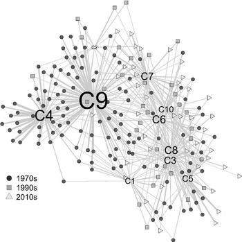
To get a deeper understanding of the links between the components, we will scrutinize them as a network, presented in Figure 4. The network is drawn based on a Fruchterman-Reingold layout (Fruchterman & Reingold, Reference Fruchterman and Reingold1991) using the igraph package in R (Csárdi, Reference Csárdi2019). The gray lines are drawn from each speaker to a component, if the probability of the component (given speaker) is more than 0.16, which was the smallest probability of a primary component in the data. Thus, the speakers might have a different number of lines drawn depending on the distribution of components. The width of the gray line represents the weight of the link: the thicker the line is between the speaker symbol and the component, the bigger the probability of the component within the interview speech. The speaker links act as springs: if a speaker uses two components, these are pulled closer together. Hence, components that are positioned close to each other tend to share a lot of speaker links. We want to emphasize that the network presentation is an approximation and optimized for readability, and different runs on the same data might result in different layouts. The nonlectal components (C2, C6, C10) are presented in the graph to preserve the original distribution between the components, but they will not be discussed in the analysis.
Network of components and speakers. Times of the interviews are presented in different shapes and shades. The width of the line presents a stronger connection. The size of the component labels corresponds to the total weight of the components’ usage in the data. The components close to each other share a lot of the same speakers.

The components that utilize more standard variants appear on the left-hand side of the figure, while the more colloquial ones are focused on the right-hand side. This divide is also apparent in the decades: most of the speakers connected to the enregistered standard (C4) and C9 were interviewed in the 1970s. Thus, the Finnish spoken in Helsinki is becoming more colloquial over the timespan of this study. The age of the speakers is not visible in Figure 4, but there are no young speakers utilizing the enregistered standard, and only eleven with C9. Conversely, in C8, C3, and especially C5, most of the speakers represent the youngest age group.
The width of the line between the speaker symbol and the component represents the proportion of the component in the speech of the informant. From the figure, we can thus interpret that C9 and especially C4 (the enregistered standard) generally explain a lot of the linguistic behavior in the interviews in which they appear. This is understandable given the standardized nature of these components. One important observation from the figure is the fact that most of the speakers tend to have more than one link. Thus, the components are used only partially. This is important, as lects have been seen as analogous to uniform systems such as languages and dialects. If, however, the speakers combine several lects in their speech, is this a wrong model?
In the previous section, we interpreted that C3 (labeled as the Southern Häme dialect) and C8 are quite similar. This is also evident in Figure 4, as they are almost overlapping. Given their similar distribution of variants and their proximity in the figure, we combine these two components to present the Southern Häme dialect. We also noted that C4, C9, and C7 form a continuum in regard to standard Finnish. This is also visible in Figure 4, and supports the division created by the LDA model: these three components are distinct enough that they should not be immediately combined. Thus, in addition to the enregistered standard (C4), we have a component that could be defined as a neutral standard (C9), and another that utilizes common colloquialisms, which we shall describe as a lax standard (C7). This raises the question of whether they represent lects or situational registers. Another issue with these three components is their use over time: in the 1970s, C4 and C9 are very frequent but seem to disappear almost completely later, whereas C7 is utilized mostly in the 1990s and 2010s. This leads us to the question of the next section: are we observing three lects or one lect changing over time?
Change in real time
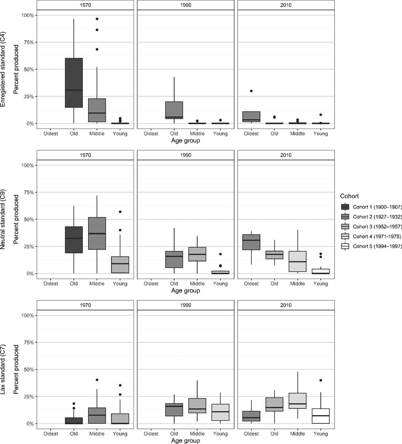
In this section, we scrutinize the components in regard to the interview rounds and the age groups. We commence with the three standard Finnish components discussed earlier, the enregistered standard (C4), the neutral standard (C9), and the lax standard (C7). The change over time in these three components is presented as a boxplot in Figure 5.
Change over time in the standard Finnish components. The cohorts and their shades correspond with Figure 2.

The enregistered standard (C4) is in strong decline, with the change happening mostly generationally. The youngest speakers in the 1970s do not use the lect or take it on later either. The middle-aged group in the 1970s preserves the usage of the lect throughout their lifespan. Among the old speakers in the 1970s, the lect is the most popular one. This was to be expected as the usage of standard Finnish as a spoken variety started in the late nineteenth century, while this group was born in the first decade of the twentieth century. The enregistered standard is thus one of the most used lects in the data, but its usage is heavily focused on the 1970s.
The neutral standard (C9) is actualized in a different pattern. Although the use of this component also decreases over time, it seems to be still actively used in the 2010s. For both the 1970s and the 1990s, the middle-aged group uses C9 the most. This would suggest an age-graded pattern: a shift toward the standard language in middle age due to pressures from the linguistic marketplace (Bourdieu & Boltanski, Reference Bourdieu and Boltanski1975; Buchstaller, Reference Buchstaller2015). This pattern does not hold in the 2010s, but, even then, the maximum values of C9 are presented in the middle-aged group. A similar pattern is visible in the lax standard (C7). The middle-aged speakers use it the most in all the decades, although in the 1990s the median of the old speakers is higher. Compared to C4 and C9, the lax standard is not as popular in the 1970s. However, in the 2010s, it is the most frequent standard Finnish component.
In conclusion, it is not easy to decide whether we should view these components as separate lects or as changing iterations of the same lect. The unique change pattern and the collection of highly salient features of the enregistered standard (C4), however, leads us to label it as a lect in its own right. C7 and C9, however, share a lot of features and a similar change pattern. There is not a clear division between these two components, and we have decided to view them as the same lect, which is based on standard Finnish but garners common colloquialisms over time.
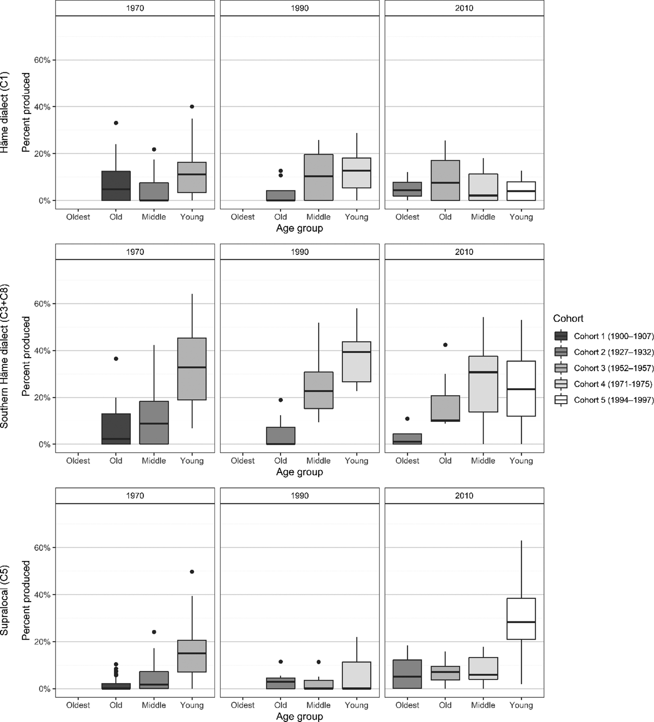
The change over time in the colloquial lects is presented in Figure 6. The Häme dialect (C1) seems to be on a generational change pattern, as the cohort born in the 1950s keeps their usage quite steady. It is, however, not popular among the young speakers in the 2010s and is thus possibly fading in Helsinki. The Southern Häme dialect (C3+C8) is very frequent among young speakers in the 1970s and 1990s but not so in the 2010s. This lect presents a retrograde change (Wagner & Sankoff, Reference Wagner and Sankoff2011) as the usage rate drops as the speakers age. The overall use, however, stays relatively steady, which means that the Southern Häme dialect is still regularly utilized in Helsinki. However, the young speakers in the 2010s do not use the Southern Häme variety as much as in the 1990s. The reason behind this is the rise of the supralocal lect (C5). The situation in the 1970s in regard to this lect is reminiscent of the Southern Häme dialect: the older the speakers, the less they use this lect. Interestingly though, the supralocal lect is used less in the 1990s than in the 1970s, and even the youngest group seems to diverge from it. Conversely, in the 2010s, it is the most popular lect among the youngest group and the older groups use it more as well. This might be due to increased mobility and the rise of social media. The popularity of the supralocal lect also suggests that some dialect leveling (Milroy, Reference Milroy2002) is happening in the community.
Change over time in the colloquial lects.

The change in real time has provided more evidence on the lects in Helsinki. Although the enregistered standard is one of the most used lects in the data, its usage is already in decline. The same is true for the Häme dialect (C1). The Southern Häme dialect, however, seems to remain constant throughout the decades. There is dialect leveling happening in the data, as the supralocal lect (C5) is the most popular among the young speakers in the 2010s, and the neutral standard (C7 + C9) utilizes some nonsalient colloquial variants as well.
Before moving on to the conclusions, we briefly comment on the sociolinguistic background variables of the speakers besides age. It is not surprising that the enregistered standard and the neutral standard are preferred by the more academic speakers, whereas the Southern Häme dialect and supralocal lect are used more by the working class. A similar difference is evident between the two neighborhoods. Interestingly, men use the Southern Häme dialect more than women, who in turn prefer the supralocal lect. Thus, the fact that the supralocal lect is gaining popularity is supported by the fact that women typically lead language change (Labov, Reference Labov1990).
CONCLUSIONS
The results presented suggest that there are coherent and distinct lects in the Finnish spoken in Helsinki. The findings contradict our initial hypothesis that the variants would show only weak covariation and that the lects would be obscure. Moreover, the lects that seemed to be the most distinct in our study were the ones that have been discussed before, both by linguists and by laymen.
Three of the components discovered by the LDA model were directly deemed to be lects (C1 as the Häme dialect, C4 as the enregistered standard, and C5 as the supralocal lect). Three components were discarded as they were more reminiscent of repeating phrases or words rather than lects. After a linguistic analysis, four of the components were combined into two: C7 and C9 to the neutral standard, and C3 and C8 to the Southern Häme dialect. Thus, ten components initially discovered by the LDA model finally led to five linguistically reasoned lects.
Earlier studies on lectal coherence have often focused on individuals (e.g., Gregersen & Pharao, Reference Gregersen and Pharao2016; Guy, Reference Guy2013). It has been noted that very few speakers are consistent in their usage of lects, and our results agree: apart from the most extreme cases of the enregistered standard, hardly any speaker uses one lect exclusively or even most of the time. This observation raises an important theoretical question: if the lects are coherent but not used in a coherent fashion, what causes the divergence?
Following Geeraerts (Reference Geeraerts, Boye and Engberg-Pedersen2010), we argue that we should not consider lects in parallel with discrete language systems, but as a network of partial systems (cf., Figure 4). Thus, the analogy between languages, dialects, and lects in general does not seem to hold true in actual usage. Whether the model of a homogeneous linguistic system is correct for languages and dialects is a question on its own and shall not be considered here. Geeraerts also argued that lects have prototype structure: each feature may be more or less typical of a certain lect. Our model has provided evidence of this: many of the variants appear in several lects but are more typical for some of them. Moreover, if we consider, for instance, the supralocal lect, none of the variants are highly typical of the lect, but it is still useful and quite popular. It must be noted that the studied features are predominantly morphophonological. This results from the agglutinative structure of Finnish, but it also means that the results might not be directly applicable to, for instance, the languages of the Indo-European family.
We have shown that the lects in Helsinki Finnish are, for the most part, constructed by coherent bundles of features. Thus, the perceptions of lects may be grounded in the linguistic reality after all. However, as hardly any speaker uses one lect invariably, it is difficult to argue that a listener could perceive a coherent lect from a single speakers’ linguistic behavior. In this regard, we approve of Gregersen and Pharao's (Reference Gregersen and Pharao2016) view of lects as being guided by salient features. Similarly, Boyd and Fraurud (Reference Boyd, Fraurud, Auer and Schmidt2010) argued that a single salient feature may suffice to label a speaker a user of Rinkeby Swedish. This is essentially what Irvine (Reference Irvine, Eckert and Rickford2001) defined as erasure: as a distinction is noted, other sociolinguistic evidence is ignored, and a homogeneous variety is imagined. A possible future study should focus on lectal perceptions based on single salient variants (cf., Campbell-Kibler, Reference Campbell-Kibler2011).
Our findings suggest that we should not consider lects and their coherence in regard to single speakers but as underlying collections of features that the speakers can incorporate in their speech. This sort of view is compatible with the idea of bricolage, as put forth by Eckert (Reference Eckert2008). Thus, considering lects as objects in their own right might be a false presumption, as they are hardly ever used in a complete manner. However, we do not encourage a model in which each variant is evaluated separately, as proposed by Guy (Reference Guy2013). We have shown that the variants indeed still covary and cluster when focusing on a larger community of speakers and that these underlying lects still offer interesting information about the relations between the variants and the people that use them. Therefore, we should not deem lects nonexistent or incoherent, but treat them as parts of an intricate system, exploited by speakers in a complex yet meaningful way.
Supplementary material
To view supplementary material for this article, please visit https://doi.org/10.1017/S0954394521000041
Acknowledgments
The research project was funded by the Kone Foundation.