1. Introduction
Richtmyer–Meshkov instability (RMI) (Richtmyer Reference Richtmyer1960; Meshkov Reference Meshkov1969) occurs when a shock wave impinges on a perturbed interface separating two different substances. This hydrodynamic instability has demonstrated critical importance in many applications (Ravid, Citron & Jeanloz Reference Ravid, Citron and Jeanloz2021; Zhou Reference Zhou2024), such as inertial confinement fusion (ICF) (Betti & Hurricane Reference Betti and Hurricane2016; Zylstra et al. Reference Zylstra2022) and supernova explosions (Abarzhi et al. Reference Abarzhi, Bhowmick, Naveh, Pandian, Swisher, Stellingwerf and Arnett2019). The baroclinic vorticity resulting from misalignment of the pressure and density gradients drives the RMI evolution (Hawley & Zabusky Reference Hawley and Zabusky1989; Jacobs et al. Reference Jacobs, Klein, Jenkins and Benjamin1993). Over the past decades, extensive researches have yielded substantial advances in RMI understanding (Zabusky Reference Zabusky1999; Brouillette Reference Brouillette2002; Ranjan, Oakley & Bonazza Reference Ranjan, Oakley and Bonazza2011; Zhou Reference Zhou2017a , Reference Zhou2017b ; Zhou et al. Reference Zhou2021, Reference Zhou, Sadler and Hurricane2025b ).
The perturbation evolution in RMI is predominantly governed by the interface parameters, such as the initial interface amplitude (Dell, Stellingwerf & Abarzhi Reference Dell, Stellingwerf and Abarzhi2015), interface wavelength (Haan Reference Haan1991) and the specific heat ratios of the fluids (Vandenboomgaerde, Mügler & Gauthier Reference Vandenboomgaerde, Mügler and Gauthier1998). Moreover, the interface Atwood number (
 $A=(\rho _d-\rho _u)/(\rho _d+\rho _u)$
, where
 $\rho _d$
and
 $\rho _u$
denote the densities of substances downstream and upstream of the interface, respectively) has been demonstrated to significantly affect the RMI growth (Dimonte & Ramaprabhu Reference Dimonte and Ramaprabhu2010). Quantifying the influence of Atwood number on RMI evolution is critically important for practical applications. In ICF, RMI directly affects the target performance optimization (Kritcher et al. Reference Kritcher2022) where different target designs employ ablator layers with different material densities, such as CH plastic versus high-density carbon (Lindl et al. Reference Lindl, Landen, Edwards, Moses and Team2014; Qiao & Lan Reference Qiao and Lan2021). Consequently, the Atwood number of key interfaces, particularly between the deuterium–tritium (DT) ice and ablator, or between successive ablative layers, varies significantly across ICF target configurations. An understanding of RMI’s Atwood-number dependence is therefore essential for predicting performance and guiding the design of ICF targets.
For single-interface RMI with small initial amplitude, postshock perturbation evolution typically progresses through distinct stages. The perturbation growth rate first increases due to the startup process (Lombardini & Pullin Reference Lombardini and Pullin2009), and then enters the linear (Richtmyer Reference Richtmyer1960) and nonlinear stages (Zhang & Guo Reference Zhang and Guo2016). The Atwood number critically influences evolution across all stages. Analytical models for the startup process (Lombardini & Pullin Reference Lombardini and Pullin2009; Li et al. Reference Li, Chen, Zhai and Luo2024b ) revealed significant Atwood-number dependence in early amplitude evolution for both light–heavy (shock propagating from light to heavy fluids) and heavy–light (shock propagating from heavy to light fluids) configurations. In the linear stage, the classical impulsive model (Richtmyer Reference Richtmyer1960) quantified effect of Atwood number for light–heavy interfaces. Vandenboomgaerde et al. (Reference Vandenboomgaerde, Mügler and Gauthier1998) generalized this by developing an empirical model (VMG model) incorporating effects of both preshock and postshock Atwood numbers, making it applicable to all single-interface RMI scenarios. The modified impulsive model proposed by Velikovich, Herrmann & Abarzhi (Reference Velikovich, Herrmann and Abarzhi2014) incorporates nonlinear corrections through a perturbation expansion method, improving predictions for initial bubble (light fluids penetrating to heavy fluids) and spike (heavy fluids penetrating to light fluids) growth rates in incompressible RMI while maintaining dependence on the Atwood number.
The above analytical models were developed under the incompressible approximation. When the compressibility effects become non-negligible in RMI flows, the reduced incompressible models like the impulsive model yield increasingly inaccurate predictions (Yang, Zhang & Sharp Reference Yang, Zhang and Sharp1994; Mikaelian Reference Mikaelian1994; Velikovich et al. Reference Velikovich, Herrmann and Abarzhi2014). To address compressibility effects, Wouchuk & Nishihara (Reference Wouchuk and Nishihara1996,Reference Wouchuk and Nishihara1997) derived analytical models (WN model) based on the compressible Euler equations, predicting linear RMI growth at both light–heavy and heavy–light interfaces. Wouchuk (Reference Wouchuk2001a , Reference Wouchuk2001b ) subsequently refined this model into a more compact form, optimizing the calculation of linear growth rates for compressible RMI. Further advancing this framework, Wouchuk & López Cavada (Reference Wouchuk and López Cavada2004) investigated perturbation oscillations induced by acoustic waves emitted from perturbed shocks. For shock–interface interactions, Cobos Campos & Wouchuk (Reference Cobos Campos and Wouchuk2016), Cobos-Campos & Wouchuk (Reference Cobos-Campos and Wouchuk2017) derived explicit analytical expansions for the asymptotic normal velocity of RMI growth by accounting for the complete history of acoustic perturbations between transmitted and reflected wavefronts. Most recently, Napieralski et al. (Reference Napieralski, Cobos, Velikovich and Huete2024) proposed a fully compressible analytic theory capturing non-decaying perturbation oscillations. This theory provides an approximate formula applicable to fluids with arbitrary equations of state, predicting asymptotic RMI growth rates and thereby extending previous models limited to ideal equations of state. The Atwood number invariably dictates linear RMI growth rates across all these compressible theories.
As nonlinearity intensifies, high-order harmonics occurs at the shocked interface (Zhang & Sohn Reference Zhang and Sohn1997). Crucially, Zhang & Sohn (Reference Zhang and Sohn1997) theoretically demonstrated a strong dependence of all harmonic amplitudes on Atwood number. Their work further quantified the growth of the spike and bubble to predict the interface mixing width. Subsequently, numerous analytical models have been developed to characterize spike/bubble evolution (Sadot et al. Reference Sadot, Erez, Alon, Oron, Levin, Erez, Ben-Dor and Shvarts1998; Mikaelian Reference Mikaelian2003; Dimonte & Ramaprabhu Reference Dimonte and Ramaprabhu2010; Nishihara et al. Reference Nishihara, Wouchuk, Matsuoka, Ishizaki and Zhakhovsky2010; Zhang & Guo Reference Zhang and Guo2022; Zhou, Zhai & Luo Reference Zhou, Sadler and Hurricane2025b ). A universal feature of these models is the fundamental role of Atwood number as a governing parameter, explicitly embedded in the expressions describing nonlinear amplitude growth.
Numerically, Dimonte & Ramaprabhu (Reference Dimonte and Ramaprabhu2010) revealed that the single-interface RMI evolution shows strong Atwood-number dependence, with spikes accelerating at high Atwood numbers due to the rapidly amplifying harmonics. Using vortex-based theory, Nishihara et al. (Reference Nishihara, Wouchuk, Matsuoka, Ishizaki and Zhakhovsky2010) analysed the distinct Atwood-number dependence patterns in planar versus cylindrical geometries. Thornber et al. (Reference Thornber, Drikakis, Youngs and Williams2010) investigated the effect of Atwood numbers on the power-law exponent of the RMI turbulent mixing width and found the distinct power-law under low- and high-Atwood-number conditions. Lombardini et al. (Reference Lombardini, Hill, Pullin and Meiron2011) considered a broad parameter space of initial Atwood number in simulations and found Atwood numbers strongly influence the turbulent kinetic energy, dissipation and postreshock mixing width growth. Experimentally, the foundational work by Meshkov (Reference Meshkov1969) established that the interface amplitude growth rate increases with Atwood numbers. While numerous experiments exploring RMI dynamics were within restricted ranges of Atwood numbers (Collins & Jacobs Reference Collins and Jacobs2002; Niederhaus & Jacobs Reference Niederhaus and Jacobs2003; Mariani et al. Reference Mariani, Vandenboomgaerde, Jourdan, Souffland and Houas2008; Vandenboomgaerde et al. Reference Vandenboomgaerde, Souffland, Mariani, Biamino, Jourdan and Houas2014; Mansoor et al. Reference Mansoor, Dalton, Martinez, Desjardins, Charonko and Prestridge2020; Li et al. Reference Li, Chen, Zhai and Luo2024a ), studies spanning a wide Atwood-number range (Motl et al. Reference Motl, Oakley, Ranjan, Weber, Anderson and Bonazza2009; Chen et al. Reference Chen, Xing, Wang, Zhai and Luo2023), consistently confirm that the perturbation growth exhibits a pronounced correlation with Atwood numbers.
Richtmyer–Meshkov instability frequently occurs at multiple fluid interfaces in practical applications. In ICF capsules, for instance, RMI develops at multiple interfaces, including the ablative front (Qiao & Lan Reference Qiao and Lan2021), the interface between the ablator and DT ice (Amendt Reference Amendt2021), and the DT ice–gas interface (Lobatchev & Betti Reference Lobatchev and Betti2000). Thus, ignition-phase RMI in ICF typically involves a layered structure with multiple interfaces rather than a single one. Compared with RMI at a single interface, the RMI evolving at a multi-interface system is affected by more complex dynamics such as reverberating waves and interface-coupling effects. For RMI at a finite-thickness layer of heavy fluid, Jacobs et al. (Reference Jacobs, Jenkins, Klein and Benjamin1995) developed a linear model to quantify the interface-coupling effect, validating it with shock-tube experiments. Mikaelian (Reference Mikaelian1996, Reference Mikaelian2005) investigated numerically and analytically the single-mode RMI evolution in both planar and cylindrical geometries for shocked layers. Theoretical analyses and numerical validations further demonstrated that RMI growth at such layers can be manipulated by modulating the initial interface morphology (Mikaelian Reference Mikaelian1996). Recent studies achieved stagnation of the downstream interface (DI) amplitude growth via modifying the upstream interface (UI) shape or the initial layer width (Sterbentz et al. Reference Sterbentz, Jekel, White, Aubry, Lorenzana and Belof2022; Chen et al. Reference Chen, Wang, Zhai and Luo2024, Reference Chen, Li, Wang, Zhai and Luo2025a ). Cong et al. (Reference Cong, Guo, Zhou, Cheng and Si2024) specifically isolated the interface-coupling mechanism by eliminating reverberating waves within the shocked heavy layer, designing conditions to stagnate perturbation growth at either UI or DI. However, for multi-interface RMI, while the effects of interface morphology and layer width have been extensively examined in prior studies, the range of Atwood numbers explored across these layer interfaces remains notably limited. While Yuan et al. (Reference Yuan, Zhao, Liu, Wang, Liu and Lu2024) numerically studied converging RMI at a cylindrical layer under varying Atwood numbers, their work prioritized validating an interface-coupling model, with discussion limited to the effect of DI Atwood number. Given the significant influence of Atwood numbers on RMI development, a thorough understanding of their impact on both the evolution of RMI and the modulation mechanisms of perturbations at a shocked layer is essential.
In summary, existing studies primarily focused on the effects of the initial shape or layer width on the RMI evolution at a shocked fluid layer. Alternatively, some works examined the influence of a wide range of Atwood numbers on the RMI evolution at a single shocked interface. However, the effect of a broad range of Atwood numbers on the evolution of a shocked layer has been rarely addressed. Across distinct Atwood-number conditions, how does interface coupling affect the RMI evolution? How can theoretical models quantify the respective effects of Atwood number of each interface on perturbation growth when both reverberating waves and interface coupling are present? Is it possible to selectively control RMI growth at UI by adjusting the Atwood number of DI, and vice versa? To address these questions, this study systematically investigates the dependence of RMI evolution on the Atwood number in a heavy fluid layer. First, following an approach similar to that of Cong et al. (Reference Cong, Guo, Zhou, Cheng and Si2024), we eliminate reverberating waves within the layer to isolate the role of the Atwood number in pure interface coupling. Second, by systematically varying the Atwood numbers to modify interface-coupling effects, we explore strategies for modulating RMI in a layer that satisfies the total-transmission condition. Third, we simulate the amplitude evolution of both the UI and DI under a range of Atwood numbers, incorporating the full influence of reverberating waves. Based on these results, we develop theoretical models to quantitatively describe how multi-interface RMI evolution depends on the Atwood numbers. Finally, with the effects of reverberating waves taken into account, we demonstrate targeted control of perturbation growth at the UI (or DI) by strategically adjusting the Atwood number of the DI (or UI).
2. Numerical methods
2.1. Numerical set-up and scheme
This work employs numerical simulations to resolve the shocked flow features and elucidate their Atwood-number dependence. The initial computational domain is shown in figure 1(a). The incident shock (IS) is positioned 10 mm upstream of the UI, and the distance between the average UI and DI positions is defined as
 $L_0$
. The system contains three gaseous media: gas 1 (upstream of the layer), gas 2 (inside the layer) and gas 3 (downstream of the layer); and gas 2 has a higher density than gases 1 and 3. Identical single-mode perturbations with wavelength
 $\lambda$
are imposed on both the UI and DI. The computational domain spans 250 mm in the
 $x$
-direction, while its width in the
 $y$
-direction equals
 $\lambda$
. Open boundary conditions are applied at the left- and right-hand boundaries, and periodic boundary conditions are used at the upper and lower boundaries. Computational efficiency is optimized by restricting calculations to a 200 mm extent along the orthogonal axes. All simulations are performed at an initial temperature of 297.8 K and pressure of 101.3 kPa. Detailed numerical settings, including the IS Mach number (
 $M_{\textit{IS}}$
), initial UI and DI amplitudes (
 $a_{1-}$
and
 $a_{2-}$
), and initial densities of the three gaseous media (
 $\rho _{10}$
,
 $\rho _{20}$
,
 $\rho _{30}$
), are presented in §§ 3–5.
The interaction between the shock and the fluid layer is governed by the two-dimensional multicomponent non-reactive Euler equations, expressed in conservative form as detailed in our prior numerical framework (Chen et al. Reference Chen, Li, Ma, Zhai and Luo2025b ). Simulations employ the high-order weighted essentially non-oscillatory (WENO) and double flux (HOWD) scheme (Ding et al. Reference Ding, Si, Chen, Zhai, Lu and Luo2017). This method combines a fifth-order WENO reconstruction (Jiang & Shu Reference Jiang and Shu1996) with the double flux algorithm (Abgrall & Karni Reference Abgrall and Karni2001; Billet & Abgrall Reference Billet and Abgrall2003) to accurately capture material interfaces and wave patterns. Time integration uses a third-order total variation diminishing Runge–Kutta scheme. The HOWD scheme has proven effective for simulating RMI at both single interfaces and layers (Li et al. Reference Li, Chen, Zhai and Luo2024b ; Cao et al. Reference Cao, Li, Wang, Zhai and Luo2024). Further implementation details are available in Ding et al. (Reference Ding, Si, Chen, Zhai, Lu and Luo2017).
Schematics of (a) the initial computational domain for a planar shock interacting with a heavy layer with two single-mode interfaces, (b) the generation of the transmitted shock (TS) inside the layer and the reflected shock (RS), (c) the flow evolution after a shock passes through a layer without reverberating waves and (d) the generation of the reverberating waves within a shocked heavy layer. Here,
 $\lambda$
and
 $L_0$
denote the perturbation wavelength and the initial layer width, respectively; IS denotes the incident shock; UI and DI represent the upstream and downstream interface of the layer, respectively; TS and RS denote the transmitted shock inside the layer and reflected shock generated by IS impacting UI, respectively; TS
 $_1$
denotes the transmitted shock moving away from the layer; RW and CW denote the rarefaction waves and compression waves within the shocked layer, respectively.

2.2. Evaluation of grid convergence and code validation
To establish mesh independence, four grid sizes (0.4, 0.2, 0.1 and 0.05 mm) are tested for a heavy fluid layer configuration with
 $\lambda =40$
mm,
 $L_0=10$
mm and dimensionless perturbation amplitudes
 $ka_{1-}=ka_{2-}=0.1$
(
 $k=2\pi /\lambda$
denotes the perturbation wavenumber), under
 $M_{\textit{IS}}=$
1.20 shock loading. The gas composition is 31.1
 $\%$
xenon/68.9
 $\%$
helium for gases 1 and 3, and 100
 $\%$
xenon for gas 2. This yields postshock Atwood numbers of
 $A_1=0.5$
at the UI and
 $A_2=-0.5$
at the DI. Notably, the compositions of specific gases in fluids 1, 2 and 3 do not evolve, demonstrating that after fixing the compositions in one case, the Atwood number is only varied by changing the density of the specific gas. Interfaces are operationally defined where the gas 2 volume fraction equals 50 %. The mixing width (
 $w$
) is the
 $x$
-direction distance between the interface nodes with the maximum and minimum
 $x$
. Temporal initialization (
 $t=0$
) corresponds to IS reaching the UI’s average position. Figure 2(a) shows the temporal evolution of
 $w$
for the UI and DI across mesh resolutions. Convergence is observed for both interfaces at 0.10 and 0.05 mm resolutions. We therefore adopt 0.10 mm to balance computational cost and accuracy.
Code validation. (a) Grid convergence verification through comparing the interface mixing width of a shocked helium/xenon/helium layer, and (b) comparison of the interface mixing width of a shocked air/SF
 $_6$
/air layer between the experiments (Li et al. Reference Li, Cao, Wang, Zhai and Luo2023) and 0.1-mesh-size numerical simulations using the domains with
 $y$
-direction width equal to
 $\lambda$
and
 $2\lambda$
.

For code validation, numerical results using the 0.1 mm mesh are benchmarked against experimental mixing width data from a shocked air/SF
 $_6$
/air layer (Li et al. Reference Li, Cao, Wang, Zhai and Luo2023), as shown in figure 2(b). The computational set-up replicates the experimental initial conditions:
 $M_{\textit{IS}}=$
1.19,
 $\lambda =60$
mm,
 $L_0=49$
mm,
 $a_{1-}=0$
mm and
 $a_{2-}=4$
mm, with 82.6 % SF
 $_6$
in the layer and pure air externally. Quantitative agreement is observed between the results from the simulation and the previous experiment. Note that the one-wavelength transverse extent of the numerical domain has the potential to restrict the growth of perturbations with wavelengths exceeding that of the fundamental mode. However, in this work, only the overall mixing width of the interface, the amplitude of the fundamental mode and the amplitudes of high-order modes with wavelengths shorter than the fundamental wavelength are extracted from the simulations and analysed. Modes with wavelengths longer than the transverse domain size are not considered in either the numerical or theoretical analysis. To verify that the one-wavelength transverse extent does not significantly affect the evolution of the interface mixing width, an additional simulation is performed using a domain with a two-wavelength transverse extent. A comparison of the results obtained from the one-wavelength and two-wavelength domains is provided in figure 2(b). The close agreement between these results confirms that the one-wavelength transverse extent has a negligible influence on the development of the interface mixing width.
3. Result and discussion
The influence of the Atwood numbers on the evolution and modulation of RMI at a layer is examined in the following four subsections, categorized by the satisfaction of the total-transmission condition. The evolution of RMI in a fluid layer is simultaneously influenced by a complex set of parameters. These include the Atwood numbers of both the upstream (
 $A_1$
) and downstream (
 $A_2$
) interfaces, the IS Mach number, the adiabatic indices of the fluids, the layer width and the initial interface geometry. To decouple the specific effects of
 $A_1$
and
 $A_2$
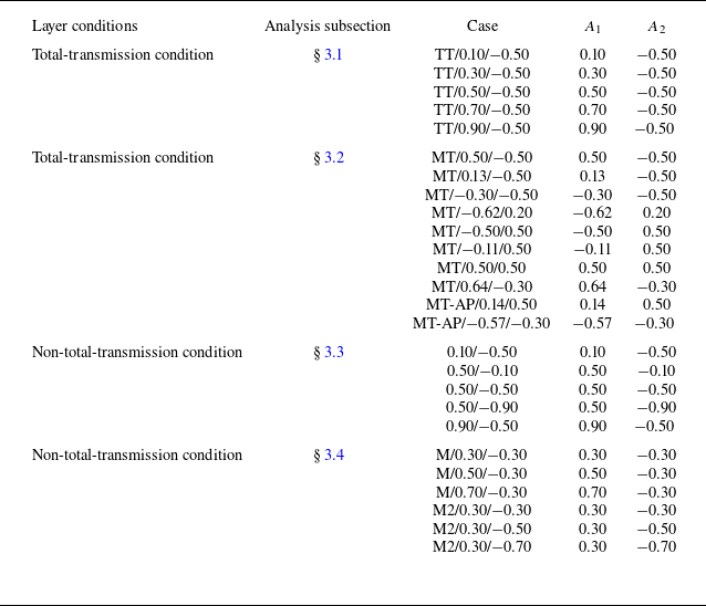
, we designed a series of distinct shock-layer configurations. The numerical cases conducted in different subsections are labelled through
 $A_1$
and
 $A_2$
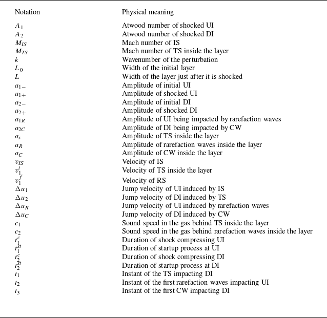
, as detailed in table 1. Note that the layer width influences the duration of the linear stage of RMI in a shocked layer. A decrease in layer width can lead to the rapid collision of RMI-induced fingers at the two interfaces, thereby accelerating the onset of nonlinear mixing. In this study, the theoretical model is derived using the potential function method, which loses validity once the two interfaces collide. As a result, layers with particularly narrow widths are not considered here. The primary quantities in the theoretical analysis are clearly defined by their physical meanings in table 2. All derived models assume single-mode perturbation dominance at the interfaces and incompressible flow.
Overview of the numerical cases run in § 3, listing the transmission condition of the layer, the subsections in which the simulations are analysed, the names of the cases and the Atwood numbers of UI (
 $A_1$
) and DI (
 $A_2$
) in each case.

Summary of notations representing the primary physical parameters in this work.

3.1. Atwood-number dependence under total-transmission condition
When the IS interacts with the UI, it generates a TS inside the layer and RS that propagates back into the upstream gas, as shown in figure 1(b). To isolate the interface-coupling effect on multi-interface RMI, reverberating waves within the layer should be eliminated. This elimination occurs when a shock passes through a gas interface satisfying the total transmission condition, a relationship between the shock Mach number and the thermophysical properties of the adjacent gases (Han & Yin Reference Han and Yin1993). The total transmission condition for the DI is given by
 \begin{equation} \frac {1+A_2}{1-A_2}=\frac {\gamma _2(\gamma _2+1)M_{\textit{TS}}^2}{\gamma _3-\gamma _2+\gamma _2(\gamma _3+1)M_{\textit{TS}}^2}, \end{equation}
where
 $M_{\textit{TS}}$
denotes the Mach number of TS, while
 $\gamma _2$
and
 $\gamma _3$
represent the adiabatic indices for gas 2 and gas 3, respectively. Equation (3.1) has been numerically validated for accuracy and reliability in prior work (Cong et al. Reference Cong, Guo, Zhou, Cheng and Si2024). Figure 1(a–c) schematically illustrate the shock-layer interaction during total transmission at the DI. Under this condition, TS traverses the DI without generating a reflecting rarefaction wave (RW), producing only a TS
 $_1$
that propagates through gas 3. This absence of RW precludes secondary reverberating waves within the layer.
In this subsection, for the total-transmission condition without reverberating waves, if
 $A_2$
is changed, the adiabatic indices of the fluids within and downstream the layer must be significantly adjusted to satisfy (3.1). Therefore, only
 $A_1$
is changed in this part to investigate the Atwood-number dependence of multi-interface RMI under total-transmission condition. To isolate the effect of
 $A_1$
, the adiabatic indices of all fluids, as well as the densities of the fluids within and downstream the layer, are held constant across all numerical cases. The initial perturbations for both interfaces are held constant, with a scaled amplitude (
 $ka$
) of 0.1 and a wavelength (
 $\lambda$
) of 40 mm. Meanwhile, the initial layer width is fixed at 10 mm. The initial upstream fluid density (
 $\rho _{10}$
) is systematically adjusted to achieve different
 $A_1$
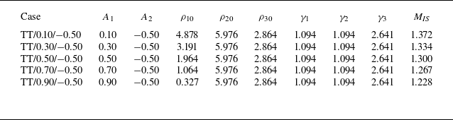
values. Critically, to maintain a consistent compression effect on the DI, the IS strength is calibrated in each case to ensure a constant Mach number for the TS within the layer. Consequently, both the initial and postshock parameters of the DI remain fixed. Under the total-transmission condition, this also results in a fixed jump velocity, which is equal for both the UI and DI. Initial conditions of numerical cases in this subsection are provided in table 3. The Mach number of TS within the layer (
 $M_{\textit{TS}}=$
1.394) is prescribed and combined with fixed
 $\gamma _2$
and
 $\gamma _3$
to satisfy (3.1). For this configuration,
 $\gamma _1=\gamma _2$
, while
 $M_{\textit{IS}}$
is derived from one-dimensional gas theory using
 $M_{\textit{TS}}=$
1.394.
Initial conditions of numerical cases in which the total transmission condition is imposed at the DI. Here
 $A_1$
(
 $A_2$
) denotes the Atwood number of the shocked UI (DI);
 $\rho _{10}$
(
 $\gamma _1$
),
 $\rho _{20}$
(
 $\gamma _2$
) and
 $\rho _{30}$
(
 $\gamma _3$
) denote the initial densities (adiabatic exponents) of gases 1, 2 and 3, respectively;
 $M_{\textit{IS}}$
denotes the IS Mach number. The unit of density is kg m
 $^{-3}$
.

Numerical schlieren images for the evolution of a shocked heavy layer without reverberating waves. The symbols have the same meaning as those in figure 1. Numbers in the schlieren images denote time with unit of
 $\unicode {x03BC}$
s.

Figure 3 presents numerical schlieren images of shocked-layer morphology for the five reverberation-free cases. Time origin is defined as the moment when IS reaches the UI average position. Using case TT/0.10/−0.50 as an example, upon TS impacting the DI, a downstream-propagating TS
 $_1$
forms in gas 3, and reverberating waves are absent within the layer (65
 $\unicode {x03BC}$
s). The late-stage evolution (1055
 $\unicode {x03BC}$
s) shows substantial morphological divergence at both UI and DI under different
 $A_1$
conditions. For the UI, its amplitude is amplified with stronger bubble/spike development at higher
 $A_1$
, which is analogous to single-interface RMI evolution (Chen et al. Reference Chen, Xing, Wang, Zhai and Luo2023). When
 $A_1=0.1$
, progressive attenuation and phase inversion (the positions of the spike and bubble at the interface have been swapped) occur for the UI perturbation (the phase of preshocked UI and DI is defined as positive hereafter). For the DI, the perturbation generally undergoes a phase reversal for cases with
 $A_1\leqslant$
0.5. In the case of TT/0.70/−0.50, the DI morphology transitions from single-mode to multimode. Notably in the case of TT/0.90/−0.50, the DI shows suppression of phase reversal with spike structures at the bubble tip. In general, in low
 $A_1$
scenarios, the DI evolution governs the flow, whereas in high
 $A_1$
scenarios, the UI growth dominates.
Comparison of the mixing width of UI (a) and DI (b) between numerical simulations and theoretical predictions for a shocked layer without reverberating waves.

The temporal evolution of mixing widths for the UI and DI are plotted in figure 4(a) and 4(b), respectively. The enhanced growth rate of the UI perturbation at higher
 $A_1$
and the complete phase reversal of the UI at
 $A_1=0.1$
are both clearly observed. The DI morphology at
 $A_1=0.7$
undergoes an incomplete phase-inversion process (non-recovery of planar geometry), and near-stagnation of the DI mixing width at
 $A_1=$
0.9 is achieved due to UI coupling. These results demonstrate strategic RMI modulation feasibility through
 $A_1$
control.
To predict the RMI evolution when interface coupling is involved, the four stages of single-mode perturbation development at a shocked single interface is referenced (Zhai et al. Reference Zhai, Chen, Xing, Li, Cao, Wang and Luo2025). In the shock compression stage, the UI amplitude can be expressed as
 \begin{equation} a_1(t)=a_{1-}-\frac {\Delta u_1}{2}\left(t+\frac {a_{1-}}{v_{\textit{IS}}}\right)\quad \quad (-t_1^c\leqslant t\leqslant t_1^{c}), \end{equation}
where
 $\Delta u_1$
denotes the jump velocity of the UI induced by IS,
 $v_{\textit{IS}}$
denotes the IS velocity and
 $t_1^{c}= {a_{1-}}/{v_{\textit{IS}}}$
represents the duration when compression of the UI is finished. After the compression stage, the startup process occurs (Lombardini & Pullin Reference Lombardini and Pullin2009) and its duration for the perturbation at the UI can be expressed as
 \begin{equation} t_1^{\textit{st}}=\frac {1}{k}\left(\frac {1-A_1}{v_1^f+\Delta u_1}+\frac {1+A_1}{v_1^{t}-\Delta u_1}\right)\!, \end{equation}
where
 $v_1^f$
is the velocity of RS induced by IS striking with the UI. For the light–heavy RMI, the amplitude growth in the startup period was quantified by Lombardini & Pullin (Reference Lombardini and Pullin2009) as
 \begin{equation} \dot {a}_{1}(t)=\frac {2\dot {a}_1^{\textit{lin}}}{(1+A_1)\coth (\textit{kL}_{{T1}})+(1-A_1)\coth (\textit{kL}_{{F1}})}\quad \quad (t_1^{c}\lt t\leqslant t_1^c+t_1^{\textit{st}}), \end{equation}
where
 \begin{equation} L_{{T1}}=(v_1^{t}-\Delta u_1)(t-t_1^c)\quad \text{and}\quad L_{F1}=({v}_1^{\textit {f}}+\Delta \textit {u}_1)(\textit {t}-\textit {t}_1^{\textit {c}}) \end{equation}
are the displacements of TS and RS, respectively, and
 $\dot {a}_1^{\textit{lin}}$
is the linear growth rate of the UI amplitude. In this work, since the gases 1, 2 and 3 are different, the linear growth rates of both the UI amplitude and the DI amplitude (
 $\dot {a}_2^{\textit{lin}}$
) can be solved based on the model proposed in our previous work (Chen et al. Reference Chen, Li, Ma, Zhai and Luo2025b
):
 \begin{equation} \begin{aligned} &\dot {a}_{1}^{\textit{lin}}[\rho _{1+}+\rho _{2+}\tanh (kL/2)]+\dot {a}_{2}^{\textit{lin}}[\rho _{3+}+\rho _{2+}\tanh (kL/2)]\\ &\quad =k\Delta u_1(\rho _{2+}-\rho _{1+})a_{1+}+k\Delta u_2[(\rho _{30}-\rho _{20})a_{2-}+(\rho _{3+}-\rho _{2+})a_{2+}]/2, \end{aligned} \end{equation}
 \begin{equation} \begin{aligned} &\dot {a}_{1}^{\textit{lin}}[\rho _{1+}+\rho _{2+}\coth (kL/2)]-\dot {a}_{2}^{\textit{lin}}[\rho _{3+}+\rho _{2+}\coth (kL/2)]\\ &\quad =k\Delta u_1(\rho _{2+}-\rho _{1+})a_{1+}-k\Delta u_2[(\rho _{30}-\rho _{20})a_{2-}+(\rho _{3+}-\rho _{2+})a_{2+}]/2. \end{aligned} \end{equation}
Here,
 $L=L_0(1-\Delta u_1/v_1^{t})$
is the layer width when TS passes through the DI and
 $\Delta u_2$
is the jump velocity of the DI induced by TS. According to the impulsive model (Richtmyer Reference Richtmyer1960) and the VMG model (Vandenboomgaerde et al. Reference Vandenboomgaerde, Mügler and Gauthier1998),
 $\rho _{1+}$
,
 $\rho _{2+}$
and
 $\rho _{3+}$
are the densities of shocked gases 1, 2 and 3, respectively. Here
 $a_{1+}=a_{1-}(1- {\Delta u_1}/{v_{\textit{IS}}})$
is the initial shocked amplitude of the UI, and
 $a_{2+}$
is the DI amplitude immediately after TS acceleration, which will be derived subsequently. Notably, the above models are applicable for perturbations with small initial amplitudes. For
 $t\gt t_1^c+t_1^{\textit{st}}$
(marking UI’s transition to nonlinear evolution), we adopt the mSEA model (Sadot et al. Reference Sadot, Erez, Alon, Oron, Levin, Erez, Ben-Dor and Shvarts1998; Xing et al. Reference Xing, Chen, Li, Wang, Zhai and Luo2025), originally developed for single-interface RMI, to quantify the nonlinear behaviour of
 $a_1$
. The mSEA formulation is
 \begin{equation} \begin{cases} \dot {a}_{1}(t)=(\dot {a}_{1b}(t)+\dot {a}_{1s}(t))/2\quad \quad (t\gt t_1^c+t_1^{\textit{st}}),\\ \dot {a}_{1b/s}(t)=\dot {a}_{1}^{\textit{lin}}\frac {1+k\dot {a}_{1}^{\textit{lin}}(t-t_1^c-t_1^{\textit{st}})}{1+(1\pm A_1)k\dot {a}_{1}^{\textit{lin}}(t-t_1^c-t_1^{\textit{st}})+F_{b/s}[k\dot {a}_{1}^{\textit{lin}}(t-t_1^c-t_1^{\textit{st}})]^2}, \end{cases} \end{equation}
where
 $F_{b/s}=3(1\pm A_1)/(2+2A_1)$
when
 $A_1\geqslant 0.5$
and
 $F_{b/s}=(1\pm A_1)/(1+A_1)$
when
 $A_1\lt 0.5$
. Combining models (3.2)–(3.8), the mixing width of the shocked UI can be theoretically predicted (
 $w_1(t)=2a_1(t)$
), as shown in figure 4(a) by lines. Good agreement between theoretical predictions and the numerical results validates the efficacy of (3.6)–(3.7) in quantifying the interface-coupling effect across diverse Atwood numbers. This agreement confirms that single-interface models (Chen et al. Reference Chen, Xing, Wang, Zhai and Luo2023; Xing et al. Reference Xing, Chen, Li, Wang, Zhai and Luo2025) successfully capture the UI’s nonlinear evolution in multi-interface systems.
The DI amplitude derivation (
 $a_2$
) accounts for TS distortion effects absent in
 $a_1$
calculations. When IS traverses UI, the TS amplitude can be expressed as
 \begin{equation} a_{s0}=a_{1-}\left(1-\frac {v_1^t}{v_{\textit{IS}}}\right)\!. \end{equation}
At
 $t_1=L_0/v_1^t$
, TS reaches DI’s average position with amplitude (
 $a_{s1}$
) being calculated by the model ((58) deduced by Bates (Reference Bates2004)). The DI compression lasts
 $2t_2^c=2(a_{2-}-a_{s1})/v_1^t$
, yielding amplitude evolution
 \begin{equation} a_2(t)=a_{2-}-\frac {\Delta u_2}{2}\left(t-t_1+\frac {a_{2-}-a_{s1}}{v_1^t}\right)\quad \quad (t_1-t_2^c\leqslant t\leqslant t_1+t_2^c). \end{equation}
Based on (3.10), the DI amplitude just after TS acceleration is expressed as
 $a_{2+}=a_{2-}- {\Delta u_2}/{v_1^t}(a_{2-}-a_{s1})$
, which can be substituted into (3.6)–(3.7). After TS passes through the DI, the duration of startup process of the DI can be calculated by the Li-model (Li et al. Reference Li, Chen, Zhai and Luo2024b
),
 \begin{equation} t_2^{\textit{st}}=\frac {1}{k}\left(\frac {1-A_2}{c_1+c_2+\Delta u_2-\Delta u_1}+\frac {1+A_2}{v_2^{t}-\Delta u_2}\right)\!, \end{equation}
where
 $v_2^{t}$
denotes TS
 $_1$
velocity in gas 3. Here
 $c_1$
and
 $c_2$
denote the sound speeds in gas 2 between the UI and TS, and between the DI and RW tail, respectively. Here,
 $c_2=c_1$
due to RW elimination. Based on the work of Li et al. (Reference Li, Chen, Zhai and Luo2024b
), the DI growth during startup period is
 \begin{equation} \dot {a}_{2}(t)=\frac {2\dot {a}_2^{\textit{lin}}}{(1+A_2)\coth (\textit{kL}_{{T2}})+(1-A_2)\coth (\textit{kL}_{{F2}})}\quad \quad (t_1+t_2^{c}\lt t\leqslant t_1+t_2^c+t_2^{\textit{st}}), \end{equation}
where
 \begin{align} L_{{T2}}=(v_2^{t}-\Delta u_2)(t-t_1-t_2^{c})\quad \text{and}\quad L_{F2}=(\textit {c}_1+\textit {c}_2+\Delta \textit {u}_2-\Delta \textit {u}_1)(\textit {t}-\textit {t}_1-\textit {t}_2^{\textit {c}})/2 \end{align}
represent the displacements of TS
 $_2$
and RW, respectively, and
 $\dot {a}_2^{\textit{lin}}$
is the linear growth rate of the DI amplitude derived from (3.6)–(3.7). After the startup process, DI’s nonlinearity is neglected due to small mixing width, as shown in figure 4(b). Actually, the mixing width of the DI is much smaller than that of the UI in cases only with large Atwood number of the UI (
 $A_1 \geqslant$
0.5). For cases with
 $A_1=$
0.3 and
 $A_1=$
0.1, the widths of both the UI and DI are comparable, but both them are small (
 $kw/2\lt$
0.3), and thus nonlinearity has very limited effects on the width evolution of both the UI and DI, as suggested by Mikaelian (Reference Mikaelian2003). As a result, the linear growth rate can quantify the amplitude evolution of the DI,
 \begin{equation} \dot {a}_{2}(t)=\dot {a}_2^{\textit{lin}}\quad \quad (t\gt t_1+t_2^c+t_2^{\textit{st}}). \end{equation}
The theoretical DI mixing widths (
 $w_2=2a_2$
) calculated from (3.9)–(3.14) are presented by lines in figure 4(b). These models effectively quantify interface-coupling effects on single-mode DI perturbations across
 $A_1$
values, with deviation only in the case with
 $A_1=0.70$
.
To reveal the origin of theory–simulation discrepancies in the case with
 $A_1=$
0.7, systematic modal decomposition of the DI perturbations is conducted and compared for cases TT/0.10/−0.50, TT/0.70/−0.50 and TT/0.90/−0.50. The fast Fourier transform (FFT) analysis of the first three harmonic modes are conducted and the temporal ratio of amplitudes of higher-order harmonics (modes 2–3) to the amplitude of basic mode
 $a_{ {basic}}$
are plotted in figure 5(a). In the case of
 $A_1=$
0.1, higher-order harmonics (modes 2–3) remain negligible, confirming the DI mixing width is governed by the fundamental mode and well-predicted by (3.9)–(3.14). A notable contrast in the relative magnitudes between the fundamental mode and high-order harmonics is observed for
 $A_1=$
0.7 and 0.9. In the case of
 $A_1=$
0.9, the fundamental mode remains significantly larger in amplitude than the second and third harmonics until
 $t=$
700
 $\unicode {x03BC}$
s. By
 $t=$
1000
 $\unicode {x03BC}$
s, however, the amplitudes of the high-order harmonics become comparable to that of the fundamental mode. As a result, theoretical predictions agree well with numerical results up to
 $t=$
700
 $\unicode {x03BC}$
s, but begin to deviate slightly by
 $t=$
1000
 $\unicode {x03BC}$
s. In contrast, for
 $A_1=$
0.7, the amplitude of the fundamental mode decreases more rapidly, allowing the growing second harmonic to surpass it around
 $t=$
700
 $\unicode {x03BC}$
s. When considering both the second and third harmonics, high-order modes significantly exceed the fundamental mode, indicating that the interface distortion is dominated by high-order harmonics. Consequently, models based solely on the fundamental mode begin to deviate from the numerical results at an earlier stage in the
 $A_1=$
0.7 case.
(a) The temporal ratios of harmonic modes amplitudes of DI to the basic mode amplitude
 $a_{ {basic}}$
at DI for cases with
 $A_1=$
0.9, 0.7 and 0.1; (b) the ratio between perturbation growth rate of the layer interfaces and the growth rate of a shocked single interface (
 $\psi$
) versus the Atwood number of the UI.

To investigate the
 $A$
-dependence of interface coupling, we introduce a normalized parameter
 $\psi$
defined as the ratio between linear amplitude growth rates of the layer interfaces calculated by (3.6) and those of shocked single interfaces calculated by the impulsive model (Richtmyer Reference Richtmyer1960) for the UI and the VMG model (Vandenboomgaerde et al. Reference Vandenboomgaerde, Mügler and Gauthier1998) for the DI. The dimensionless quantity
 $\psi$
of the UI (
 $\psi _1$
) and the DI (
 $\psi _2$
) are formulated as
 \begin{equation} \begin{cases} \psi _1=\dot {a}_{1}^{\textit{lin}}/(ka_{1+}A_1\Delta u_1),\\ \psi _2=\dot {a}_{2}^{\textit{lin}}/[k\Delta u_2(a_{2+}A_2+a_{2-}A_{20})/2], \end{cases} \end{equation}
where
 $A_{20}=(\rho _{30}-\rho _{20})/(\rho _{30}+\rho _{20})$
is the Atwood number of the DI prior to shock passage.
The calculated
 $\psi$
of the two interfaces versus
 $A_1$
is presented in figure 5(b). The absolute values of both
 $\psi _1$
and
 $\psi _2$
remain universally below 1 across
 $A_1$
variations, demonstrating that the interface coupling suppresses the amplitude growth for both the UI and DI in this work. With
 $A_1$
increasing from 0.1 to 0.9, the interface-coupling effects for the two interfaces exhibit monotonic dependence on
 $A_1$
. For the light–heavy perturbation at the UI, its growth exhibits phase reversal at low
 $A_1$
(approximately
 $A_1\lt$
0.15) due to interface coupling relative to the perturbation in the single-interface condition. As
 $A_1$
decreases, the term
 $ka_{1+}A_1\Delta u_1$
decreases in magnitude. This leads to a more sensitive variation in
 $\psi _1$
as
 $A_1$
changes, primarily by modulating
 $\dot {a}_{1}^{\textit{lin}}$
. When
 $A_1$
becomes sufficiently small, the intrinsic perturbation growth at a single UI becomes negligible. In this regime, the coupling between interfaces dominates over the perturbation growth at UI. At high
 $A_1$
, the UI amplitude growth rate asymptotically approaches the rate in the single-interface condition. For the heavy–light perturbation at the DI, its growth closely approximates the single-interface condition at low
 $A_1$
, which means that the DI morphology is dominated by the fundamental harmonic. As
 $A_1$
increases, the decreasing
 $\psi _2$
indicates that the basic mode decays in the early stage with a suppressing rate compared with the single-interface condition, leading to the DI morphology being dominated by the high-order harmonics soon. Under high
 $A_1$
(approximately
 $A_1\gt$
0.87) conditions,
 $\psi _2\lt 0$
, the interface coupling eliminates the phase reversal of the DI perturbation, which explains the initially growing DI fundamental mode in
 $A_1=$
0.9. As a result, effects of
 $A_1$
on the DI perturbation growth may be distinguished into three different phases, but their boundaries are not clear now.
Pressure gradient of the flow near the UI at the moment when TS just forms in the layer (a), and the flow near the layer after TS passes through the DI (b). The red and blue dotted lines represent the position of UI and DI, respectively.

Moreover, as revealed in previous works (Wouchuk & López Cavada Reference Wouchuk and López Cavada2004; Calvo-Rivera, Velikovich & Huete Reference Calvo-Rivera, Velikovich and Huete2023; Napieralski et al. Reference Napieralski, Cobos, Velikovich and Huete2024), after the IS passes the UI, the resulting perturbed TS propagates through the layer and radiates perturbed acoustic waves back towards the UI to establish mechanical equilibrium. These acoustic waves reverberate within the layer and influence perturbation growth at both the UI and DI, as indicated by the oscillatory behaviour observed in the growth curves in figure 4. As a result, studying the Atwood-number dependence of these acoustic waves is essential for a thorough understanding of RMI evolution in a layered configuration. To isolate the effect of the Atwood number on perturbed acoustic waves without interference from zero-order reflected waves, we analyse behaviour of acoustic waves under total-transmission condition. The propagation of acoustic waves within the layer is visualized by extracting the pressure gradient
 $|\boldsymbol{\nabla }p|$
in the flow near the interfaces. For the numerical cases with varying
 $A_1$
, we focus on two key instants: the moment when the TS is initially generated inside the layer, and the time when this shock just departs from the DI, as illustrated in figures 6(a) and 6(b), respectively.
As shown in figure 6(a), an increase in
 $A_1$
leads to a stronger pressure disturbance propagating from the shocked UI towards the DI. This indicates that a higher
 $A_1$
amplifies the initial acoustic waves, which in turn influence the subsequent RMI evolution at the DI. After the shock fully traverses the layer (figure 6
b), the reverberating acoustic waves remain weak and barely observable at low
 $A_1$
values. However, as
 $A_1$
exceeds 0.5, these waves coalesce into a conspicuous, single-mode wave system inside the layer. This coherent wave structure, which grows increasingly prominent with higher
 $A_1$
, exhibits stronger pressure gradients and occupies a broader region, exerting a significant influence on the evolution of both the DI and UI.
In the present study, the IS is relatively weak and all fluid media are gaseous. Under these conditions, the incompressible flow models employed in our derivations provide reasonably accurate predictions for both the linear and nonlinear growth of perturbations at the shocked layer. Given the good agreement observed between these model predictions and the numerical results, a quantitative modelling of the acoustic wave propagation and its influence on the RMI is not pursued in this work. Nevertheless, it is recognized that the incompressible theory becomes increasingly inaccurate when compressibility effects are significant, such as in scenarios involving strong IS. In future studies, we intend to adopt a compressible theoretical framework to quantitatively analyse the role of acoustic waves in modulating the amplitude evolution. A model capable of accurately quantifying the acoustic wave effects in multi-interface RMI under strong shock conditions is expected to develop.
In summary, at lower
 $A_1$
, interface coupling exerts a significantly more pronounced influence on the UI than on the DI, and causes phase reversal to occur in light–heavy UI where it normally should not manifest. Conversely, at higher
 $A_1$
, interface coupling has a much stronger effect on the DI than on the UI, and prevents phase reversal from occurring in heavy–light DI where it normally would be expected. Furthermore, there is a critical
 $A_1$
yielding
 $\psi =0$
for either the UI or DI, revealing that when reverberating waves are eliminated, the freeze-out can be achieved at either the UI or DI under a specific Atwood-number condition of the layer.
3.2. Modulation of RMI under total-transmission condition
Systematic variation of the initial layer width modulates RMI growth in shocked layer with a perturbed interface and planar interface through reverberating waves (Zhou et al. Reference Zhou, Zhai and Luo2025a
; Chen et al. Reference Chen, Li, Wang, Zhai and Luo2025a
). For the layer with two perturbed interfaces, conventional RMI control relies on specific UI/DI amplitude combinations (Mikaelian Reference Mikaelian1996; Sterbentz et al. Reference Sterbentz, Jekel, White, Aubry, Lorenzana and Belof2022; Liang & Luo Reference Liang and Luo2023; Cong et al. Reference Cong, Guo, Zhou, Cheng and Si2024). However, precise fabrication of such amplitude/wavelength configurations proves impractical for ICF targets (Mikaelian Reference Mikaelian1996). By selecting ablative materials, the Atwood numbers of interfaces in ICF targets can be effectively controlled. This alteration of Atwood numbers may enable direct tuning of RMI growth during ignition. In order to figure out the approach of modulating multi-interface RMI via adjusting Atwood numbers and the parameters defining the modulation of perturbation growth at a shocked layer, we derive the following two dimensionless expressions for the linear growth rates of the UI amplitude (
 $a_1$
) and DI amplitude (
 $a_2$
) by further developing (3.6)–(3.7):
 \begin{equation} \frac {\dot {a}_{1}^{\textit{lin}}}{k\Delta u_1a_{1+}}=\frac {A_1(1+A_2)+A_1(1-A_2)\coth (k*L) +\alpha A_2(1+A_1)\mathrm{csch}(kL)}{1-A_1A_2+(1+A_1A_2)\coth {(kL)}}, \end{equation}
 \begin{equation} \frac {\dot {a}_{2}^{\textit{lin}}}{k\Delta u_1a_{1+}}=\frac {\alpha A_2(1-A_1)+\alpha A_2(1+A_1)\coth (k*L) +A_1(1-A_2)\mathrm{csch}(kL)}{1-A_1A_2+(1+A_1A_2)\coth {(kL)}}. \end{equation}
Here,
 $\alpha = {(\rho _{30}-\rho _{20})\Delta u_2 a_{2-}+(\rho _{3+}-\rho _{2+})\Delta u_2a_{2+}}/{2(\rho _{3+}-\rho _{2+})\Delta u_1a_{1+}}$
, which mainly reflects the ratio of amplitudes of two interfaces. Based on the derived model, the modulation of RMI at a fluid layer can be characterized by four dimensionless parameters:
 $A_1$
,
 $A_2$
,
 $\alpha$
and
 $kL$
. Notably, this model is applicable to a shocked layer under total-transmission condition. By fixing
 $\alpha =0.78$
and
 $kL=1.21$
, consistent with the conditions in case TT/0.50/−0.50, we use the model to establish the relationships between
 $A_1$
and
 $A_2$
required to achieve perturbation growth stagnation at either the UI or DI. This relationship is illustrated in the figure 7(a). These two curves in the figure are defined as the freezing lines, which means the perturbation growth stagnation can be realized at either the UI or DI when the (
 $A_2$
,
 $A_1$
) coordinate locates at these two characteristic curves.
(a) Distribution of the manipulation possibilities of the perturbation growth at the UI and DI in (
 $A_2$
,
 $A_1$
) domain; (b) schematics of the temporal evolution of UI and DI amplitudes in the eight possibilities.

Based on figure 7(a) and extensive additional calculations under various combinations of
 $\alpha$
and
 $kL$
, it is observed that the curves corresponding to RMI freeze-out at the UI and DI always intersect at (
 $A_2=$
0,
 $A_1=$
0). This indicates that simultaneously freezing perturbation growth at both interfaces by adjusting only the Atwood numbers, at a layer under total-transmission condition, is theoretically unattainable. The two curves in figure 7(a) delineate eight distinct regimes of RMI modulation possibilities, categorized by the direction of amplitude growth at the UI and DI. The temporal amplitude evolution of both UI and DI for the eight possibilities are sketched in figure 7(b). By systematically selecting
 $A_2$
and
 $A_1$
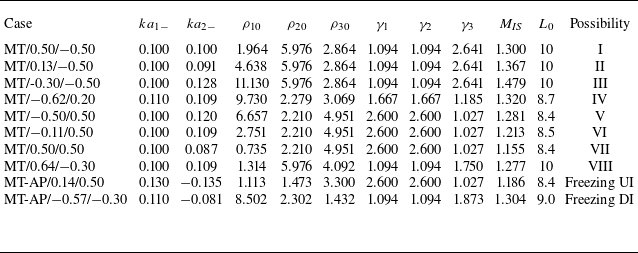
values in the initial configurations, we conduct eight numerical simulations to realize each of these modulation scenarios. The initial settings of the eight cases corresponding to different possibilities are detailed in table 4 and the corresponding amplitude evolutions of both interfaces, extracted from these simulations, are presented in figure 8. The wavelength of perturbation in all the simulations is 40 mm. The different initial scaled interface amplitudes (
 $ka_1$
and
 $ka_2$
) and layer widths (
 $L_0$
) are set to fix the dimensionless parameter
 $\alpha$
and layer width when TS impacting DI (
 $L=L_0(1-\Delta u_1/v_1^t)$
). Results confirm that all eight modulation possibilities are successfully reproduced in the simulations and align closely with the predictions of the models (3.16)–(3.17). It should be noted that the defined modulation possibilities encompass not only the case of a shocked heavy layer (
 $A_2\lt 0$
and
 $A_1\gt 0$
) but also layers with all other possible combinations of
 $A_2$
and
 $A_1$
.
Initial conditions of numerical cases for realizing different possibilities of RMI growth at an in-phase layer and freezing perturbation growth at interfaces of an antiphase layer under the total-transmission condition. Here
 $ka_{1-}$
and
 $ka_{1-}$
are the initial scaled amplitudes of UI and DI, respectively. The symbols have the same meaning as those in table 3. The units of density and width are kg m
 $^{-3}$
and mm, respectively.

Temporal amplitude evolution of both the UI and DI in the simulations designed for the eight different modulation possibilities of RMI at an in-phase layer.

To further validate the universality of our models, we also simulate cases involving layers with antiphase initial perturbations (
 $\alpha \lt 0$
), as detailed in table 4. With
 $\alpha$
and
 $kL$
set to −0.78 and 1.21 respectively, two specific combinations of
 $A_2$
and
 $A_1$
, predicted by the dimensionless models (3.16)–(3.17) to induce RMI stagnation at either the UI or DI, are numerically tested. The computed perturbation amplitude evolutions for both interfaces are plotted in the figure 9. As evidenced by the results, amplitude growth stagnation is successfully achieved at the targeted interface in each case, confirming the model’s capability to accurately predict stagnation conditions in initially antiphase layers.
3.3. Atwood-number dependence under non-total-transmission condition
In practical scenarios, the total transmission condition is unattainable, resulting in persistent wave reverberations within the shocked layer. For shock-accelerated heavy layers, as shown in figure 1(d), these reverberation waves comprise RW generated when TS impacts DI and CW reflected from RW–UI interaction. Similar to that in § 3.1, the initial perturbations for both interfaces are with fixed
 $ka=0.1$
and
 $\lambda =$
40 mm, and the initial layer width
 $L_0=$
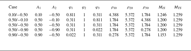
10 mm. To investigate the Atwood-number dependence of multi-interface RMI in a heavy layer with reverberating waves, we conduct simulations in which both
 $A_1$
and
 $A_2$
were systematically varied. In all cases for this part, the adiabatic index is set to 1.67. For investigating
 $A_1$
dependence, the initial configurations are set similarly to those in the preceding part: the upstream fluid density (
 $\rho _{10}$
) is altered to vary
 $A_1$
, while the densities of the other fluids are maintained. Concurrently, the IS Mach number is adjusted in each case to ensure a constant TS Mach number within the layer, thereby isolating the
 $A_1$
effect from changes in shock compressing DI. For investigating
 $A_2$
dependence, the densities of the fluids upstream and within the layer are held constant, fixing
 $A_1$
. The downstream fluid density is then varied to achieve different
 $A_2$
values. In these simulations, the IS Mach number is fixed at 1.20. This configuration ensures that the initial jump velocities of both interfaces remain unchanged across cases, allowing the observed differences to be attributed solely to
 $A_2$
. The complete set of initial parameters for these cases is provided in table 5. The cases are labelled as
 $A_1/A_2$
to denote Atwood-number combinations.
Initial parameters of the numerical cases designed to investigate the Atwood-number dependence of RMI at a helium/xenon/helium layer with reverberating waves. Here
 $\varphi _1$
,
 $\varphi _2$
and
 $\varphi _3$
denote the volume fractions of xenon in gases 1, 2 and 3, respectively; 1-
 $\varphi _1$
, 1-
 $\varphi _2$
and 1-
 $\varphi _3$
denote the volume fractions of helium in gases 1, 2 and 3, respectively.

Amplitude evolution of the interfaces of an initial antiphase layer in the simulations designed for realizing RMI stagnation at the UI (a) and DI (b).

Figure 10 presents schlieren images of layer evolution for all five reverberating-wave cases. Wave structures resemble those in figure 3, with notable RW emerging from TS–DI interactions. Following shock traversal through the layer, both the UI and DI remain single-mode. At the late stage, the perturbation growth exhibits pronounced sensitivity to
 $A_1$
and
 $A_2$
. When
 $A_2$
is fixed, the DI mixing width inversely correlates with
 $A_1$
, while DI transitions to multimode morphology at higher
 $A_1$
. The UI exhibits accelerated growth and enhanced nonlinearity (bubbles, spikes, roll-ups) with increasing
 $A_1$
. When
 $A_1$
is fixed, the UI mixing widths remain comparable, but asymmetry intensifies with
 $A_2$
increasing. Specifically, the roll-up structures form at the UI spike when
 $A_2=-$
0.9. The DI amplitude grows with higher
 $A_2$
, and the phase inversion is suppressed when
 $A_2=-$
0.1. Similar to the UI, the DI asymmetry accelerates at higher
 $A_2$
.
Schlieren images of the shock-induced helium/xenon/helium layer evolution under different Atwood-number conditions.

Given the absence of theoretical frameworks for harmonic evolution in shocked layers and the persistent dominance of basic modes, as shown in figure 10, we analyse basic-mode growth at the UI and DI via FFT analysis, as presented in figure 11. For the UI of a heavy layer, both IS and RW induce acceleration directed from light to heavy fluids. Therefore, assuming the initial UI phase is defined as positive, the effects of both IS and RW on the UI amplitude are positive. The accelerations of the DI induced by TS and CW within the layer are both from heavy to light fluids, indicating that the effects of TS and CW on the DI amplitude are negative. Figure 11(b) shows that for the DI, the intensified interface coupling at elevated
 $A_1$
causes the basic mode amplitude of the DI to grow into a negative phase at an attenuated rate. This behaviour aligns with the phenomenology observed in figure 4. In case 0.10/−0.5, the fundamental mode amplitude at the UI evolves to the negative phase. This occurs because the interface-coupling effect overcomes the positive effects of IS and RW. However, for cases 0.50/−0.5 and 0.90/−0.5, the perturbation amplitude on the UI increases consistently, governed by the dominant effects of IS and RW. Figure 11(d) reveals that in case 0.50/−0.10, the fundamental mode of the DI evolves to a positive phase. This results from interface coupling governing the fundamental mode of the DI. When
 $A_1$
and
 $M_{\textit{IS}}$
are fixed as 0.5 and 1.2, respectively, the effect of IS on the UI perturbation remains constant. Therefore, the non-monotonic relationship between
 $A_2$
and the UI amplitude growth rate observed in figure 11 results from mutual cancellation between the RW effect and the interface coupling contribution.
Comparison of the fundamental mode amplitude between numerical results (symbols) and predictions (lines matching the colour of the symbols) from models incorporating two reverberating waves for UI and DI in cases with fixed
 $A_2$
(a,b) and cases with fixed
 $A_1$
(c,d). The pink lines in (c) and (d) denote the theoretical predictions from models incorporating four reverberating waves.

To quantify the coupled effects of wave reverberating and interface coupling on multi-interface RMI across varying Atwood-numbers, we adopt a linear model. In our prior work (Chen et al. Reference Chen, Li, Ma, Zhai and Luo2025b ), the models incorporating different interface accelerations arising from reverberating waves inside a shocked three-fluids layer, are expressed as
 \begin{equation} \begin{cases} \begin{aligned} &\frac {{{d}}^{2}a_1}{{{d}}t^{2}}[\rho _1+\rho _2\tanh (kL/2)]+\frac {{{d}}^{2}a_2}{{{d}}t^{2}}[\rho _3+\rho _2\tanh (kL/2)]\\ &\quad =k[(\rho _2-\rho _1)a_1g_1+(\rho _3-\rho _2)a_2g_2], \\ &\frac {{{d}}^{2}a_1}{{{d}}t^{2}}[\rho _1+\rho _2\coth (kL/2)]-\frac {{{d}}^{2}a_2}{{{d}}t^{2}}[\rho _3+\rho _2\coth (kL/2)]\\ &\quad =k[(\rho _2-\rho _1)a_1g_1-(\rho _3-\rho _2)a_2g_2]. \end{aligned} \end{cases} \end{equation}
When both the UI jump velocities induced by IS (
 $\Delta u_1$
) and RW (
 $\Delta u_{\textit{R1}}$
), and DI jump velocities induced by TS (
 $\Delta u_2$
) and CW (
 $\Delta u_{{C1}}$
) are considered,
 $g_1$
and
 $g_2$
can be expressed as
 \begin{equation} \begin{cases} g_1=\Delta u_1\delta t+\Delta u_{\textit{R1}}\delta (t-t_2), \\ g_2=\Delta u_2\delta (t-t_1)+\Delta u_{{C1}}\delta (t-t_3), \end{cases} \end{equation}
where
 $t_2$
and
 $t_3$
are the instants when RW arrive at the UI and CW interact with the DI, respectively, and are expressed as
 \begin{equation} \begin{cases} t_2=t_1+L_0(1-\Delta u_1/v_1^t)/c_1, \\ t_3=t_2+L_0(1-\Delta u_1/v_1^t)[1+(\Delta u_2-\Delta u_1)/c_1]/c_2. \end{cases} \end{equation}
By substituting (3.19) into (3.18) and applying the impulsive model to IS-driven UI acceleration and the VMG model to TS-driven DI acceleration, we integrate (3.18) to establish linear growth models for the fundamental mode amplitudes of the UI and DI:
 \begin{align} \begin{aligned} &\dot {a}_{1}^{\textit{lin}}[\rho _{{1R}}+\rho _{{2R}}\tanh (kL/2)]+\dot {a}_{2}^{\textit{lin}}[\rho _{{3C}}+\rho _{{2C}}\tanh (kL/2)]\\ &\quad =k\Delta u_1(\rho _{2+}-\rho _{1+})a_{1+}+k\Delta u_{\textit{R1}}(\rho _{{2R}}-\rho _{{1R}})a_{{1R}}\\ &\qquad +k\Delta u_2[(\rho _{30}-\rho _{20})a_{2-}+(\rho _{3+}-\rho _{2+})a_{2+}]/2+k\Delta u_{{C1}}(\rho _{{3C}}-\rho _{{2C}})a_{{2C}}, \end{aligned} \\[-28pt] \nonumber \end{align}
 \begin{align} \begin{aligned} &\dot {a}_{1}^{\textit{lin}}[\rho _{{1R}}+\rho _{{2R}}\coth (kL/2)]-\dot {a}_{2}^{\textit{lin}}[\rho _{{3C}}+\rho _{{2C}}\coth (kL/2)]\\ &\quad =k\Delta u_1(\rho _{2+}-\rho _{1+})a_{1+}+k\Delta u_{\textit{R1}}(\rho _{{2R}}-\rho _{{1R}})a_{{1R}}\\ &\qquad -k\Delta u_2[(\rho _{30}-\rho _{20})a_{2-}+(\rho _{3+}-\rho _{2+})a_{2+}]/2-k\Delta u_{{C1}}(\rho _{{3C}}-\rho _{{2C}})a_{{2C}}. \end{aligned} \\[2pt] \nonumber \end{align}
Here
 $\rho _{{1R}}$
and
 $\rho _{{2R}}$
denote the densities of gases 1 and 2 after RW hit the UI, respectively;
 $\rho _{{2C}}$
and
 $\rho _{{3C}}$
denote the densities of gases 2 and 3 after CW impact the DI, respectively;
 $a_{1+}$
(the UI amplitude post-IS acceleration) and
 $a_{2+}$
(the DI amplitude post-TS acceleration) can be calculated via equations in § 3.1;
 $a_{{1R}}$
denotes the UI amplitude immediately after RW impact. Accounting for the startup process, the UI amplitude prior to RW impact is given by
 \begin{equation} \begin{cases} a_{{1R-}}=a_{1+}+\int _{t_1^c}^{t_2}\frac {2\dot {a}_1^{\textit{lin}}}{(1+A_1)\coth (\textit{kL}_{{T1}})+(1-A_1)\coth (\textit{kL}_{{F1}})}\text{d}t\\ ( t_2\lt t_1^c+t_1^{\textit{st}}),\\ a_{{1R-}}=a_{1+}+\int _{t_1^c}^{t_1^c+t_1^{\textit{st}}}\frac {2\dot {a}_1^{\textit{lin}}}{(1+A_1)\coth (\textit{kL}_{{T1}})+(1-A_1)\coth (\textit{kL}_{{F1}})}\text{d}t+(t_2-t_1^c-t_1^{\textit{st}})\dot {a}_1^{\textit{lin}}\\(t_2\geqslant t_1^c+t_1^{\textit{st}}). \end{cases} \end{equation}
Here,
 $t_1^{\textit{st}}$
,
 $L_{{F1}}$
and
 $L_{{T1}}$
are defined in (3.3)–(3.5). To quantify RW–UI interaction, we consider RW amplitude dynamics. When RW originate from TS impacting the DI, the initial RW amplitudes are
 \begin{equation} \begin{cases} a_{{{R0}}}=(a_{{{Rf0}}}+a_{{{Rt0}}})/2,\\ a_{{{Rf0}}}=a_{2-}-(a_{2-}-a_{s1})(c_1-\Delta u_1)/v_1^t,\\ a_{{{Rt0}}}=a_{2-}-(a_{2-}-a_{s1})(c_2-\Delta u_2)/v_1^t, \end{cases} \end{equation}
where
 $c_1$
and
 $c_2$
denote sound speeds in gas 2 (RW front to the UI and RW tail to the DI regions, respectively),
 $a_{s1}$
is given by (3.9). The RW tail amplitude evolves during moving within the layer as (Velikovich & Phillips Reference Velikovich and Phillips1996)
 \begin{equation} \dot {a}_{{{Rt}}}=-ka_{{{Rf0}}}c_1\sqrt {(\gamma _2+1)(1-c_2/c_1)/(\gamma _2-1)}. \end{equation}
Since the RW front amplitude remains constant, the RW amplitude at the moment of impacting UI is
 \begin{equation} a_{{R1}}=a_{{{R0}}}+\dot {a}_{{{Rt}}}(t_2-t_1)/2. \end{equation}
Based on (3.23)–(3.26), the UI amplitude immediately after RW impact can be expressed as
 \begin{equation} a_{{1R}}=a_{{1R-}}+(a_{{1R-}}-a_{{R1}})\frac {\Delta u_{\textit{R1}}}{c_1+c_2+\Delta u_1-\Delta u_2}. \end{equation}
In (3.21)–(3.22),
 $a_{{2C}}$
(the DI amplitude post-CW impact) incorporates the DI startup process,
 \begin{equation} \begin{cases} a_{{2C-}}=a_{1+}+\int _{t_1+t_2^c}^{t_3}\frac {2\dot {a}_2^{\textit{lin}}}{(1+A_2)\coth (\textit{kL}_{{T2}})+(1-A_2)\coth (\textit{kL}_{{F2}})}\text{d}t\\ ( t_3\lt t_1+t_2^c+t_2^{\textit{st}}),\\ a_{{2C-}}=a_{1+}+\int _{t_1+t_2^c}^{t_1+t_2^c+t_2^{\textit{st}}}\frac {2\dot {a}_2^{\textit{lin}}}{(1+A_2)\coth (\textit{kL}_{{T2}})+(1-A_2)\coth (\textit{kL}_{{F2}})}\text{d}t+(t_3-t_1-t_2^c-t_2^{\textit{st}})\dot {a}_2^{\textit{lin}}\\(t_3\geqslant t_1+t_2^c+t_2^{\textit{st}}), \end{cases} \end{equation}
where
 $t_2^{\textit{st}}$
,
 $L_{{F2}}$
and
 $L_{{T2}}$
are defined in (3.11)–(3.13). The CW amplitude after reflection by RW interacting with the UI is
 \begin{equation} \begin{cases} a_{{{C0}}}=(a_{{{Cf0}}}+a_{{{Ct0}}})/2,\\ a_{{{Cf0}}}=a_{{1R-}}-(a_{{1R-}}-a_{{Rf0}})(c_2+\Delta u_2-\Delta u_1)/c_1,\\ a_{{{Ct0}}}=a_{{1R-}}-[a_{{1R-}}-a_{{Rt0}}-\dot {a}_{{{Rt}}}(t_2-t_1)](c_3+\Delta u_{\textit{R1}})/c_2. \end{cases} \end{equation}
Here,
 $a_{{1R-}}$
,
 $a_{{Rt0}}$
,
 $a_{{Rf0}}$
and
 $\dot {a}_{{{Rt}}}$
are calculated from (3.23)–(3.25);
 $c_3$
is the sound speed of gas 2 between CW tail and the UI. Given the CW’s weakness and brief transit, its amplitude variation is neglected. The DI amplitude after CW passage is
 \begin{equation} a_{{2C}}=a_{{2C-}}-(a_{{2C-}}-a_{{C0}})\frac {2\Delta u_{{C1}}}{c_3+c_2+\Delta u_{\textit{R1}}+\Delta u_1-\Delta u_2}. \end{equation}
In conclusion, (3.21)–(3.30) determine the linear growth rates for the UI and DI amplitudes.
As shown in figure 11, the theoretically predicted curves exhibit strong agreement with numerical results during the linear stage, excepting the maximum
 $A_2$
configuration. For case 0.50/−0.90 (figure 11
c,d), the green theoretical lines derived from (3.21)–(3.22) display significant divergence from simulated UI amplitudes. Because a high amplitude of
 $A_2$
intensifies reverberating waves generated by wave–DI interactions, the deviation in (3.21)–(3.22) stems from neglecting additional reflected waves within the layer during derivation.
Comparison of the interface velocities in the
 $x$
-direction of the shocked heavy layer between the numerical results (symbols) and predictions (lines) from one-dimensional gas theory for case 0.90/−0.50 (a) and case 0.50/−0.90 (b).

Figures 12(a) and 12(b) show temporally averaged
 $x$
-direction velocities of interface nodes from cases 0.90/−0.50 and 0.50/−0.90, respectively. Dotted lines represent one-dimensional gas theory predictions considering only RW and CW. Note that based on the constraints in numerically extracting flow parameters with limited temporal resolution, the simulated results cannot precisely capture the ideal instantaneous velocity jumps at the interfaces. As a result, deviations from the one-dimensional ideal-gas theory may occur during the very brief period of wave–interface interactions. The final interface velocity, which stabilizes after approximately 400
 $\unicode {x03BC}$
s, reflects the cumulative effect of velocity jumps induced by all relevant wave–interface interactions. For high
 $A_1$
configurations (figure 12
a), the second gas theory (incorporating first and second reflected waves) accurately predicts the UI and DI velocities. However, for enhanced
 $A_2$
cases (figure 12
b), this theory shows discrepancies, particularly for the UI. Thus, accurate acceleration prediction for high-
 $A_2$
layers requires additional reverberating waves. Solid lines in figure 12(b) show fourth gas theory predictions incorporating four waves: RW, CW, RW
 $_2$
(rarefaction waves from CW-DI interaction) and CW
 $_2$
(from RW
 $_2$
-UI interaction). This fourth gas theory accurately predicts the UI and DI accelerations for case 0.50/−0.90. We therefore reformulate (3.21)–(3.22) as
 \begin{equation} \begin{aligned} &\dot {a}_{1}^{\textit{lin}}[\rho _{{1R}}+\rho _{{2R}}\tanh (kL/2)]+\dot {a}_{2}^{\textit{lin}}[\rho _{{3C}}+\rho _{{2C}}\tanh (kL/2)]\\ &=k\Delta u_1(\rho _{2+}-\rho _{1+})a_{1+}+k\Delta u_{\textit{R1}}(\rho _{{2R}}-\rho _{{1R}})a_{{1R}}+k\Delta u_{\textit{R2}}(\rho _{{2R2}}-\rho _{{1R2}})a_{{1R2}}\\ &\quad +k\Delta u_2[(\rho _{30}-\rho _{20})a_{2-}+(\rho _{3+}-\rho _{2+})a_{2+}]/2\\ &\quad +k\Delta u_{{C1}}(\rho _{{3C}}-\rho _{{2C}})a_{{2C}}+k\Delta u_{{C2}}(\rho _{{3C2}}-\rho _{{2C2}})a_{{2C2}}, \end{aligned} \end{equation}
 \begin{equation} \begin{aligned} &\dot {a}_{1}^{\textit{lin}}[\rho _{{1R}}+\rho _{{2R}}\coth (kL/2)]-\dot {a}_{2}^{\textit{lin}}[\rho _{{3C}}+\rho _{{2C}}\coth (kL/2)]\\ &=k\Delta u_1(\rho _{2+}-\rho _{1+})a_{1+}+k\Delta u_{\textit{R1}}(\rho _{{2R}}-\rho _{{1R}})a_{{1R}}+k\Delta u_{\textit{R2}}(\rho _{{2R2}}-\rho _{{1R2}})a_{{1R2}}\\ &\quad -k\Delta u_2[(\rho _{30}-\rho _{20})a_{2-}+(\rho _{3+}-\rho _{2+})a_{2+}]/2\\ &\quad -k\Delta u_{{C1}}(\rho _{{3C}}-\rho _{{2C}})a_{{2C}}-k\Delta u_{{C2}}(\rho _{{3C2}}-\rho _{{2C2}})a_{{2C2}}, \end{aligned} \end{equation}
where
 $\Delta u_{\textit{R2}}$
(
 $\Delta u_{{C2}}$
),
 $\rho _{{1R2}}$
and
 $\rho _{{2R2}}$
(
 $\rho _{{2C2}}$
and
 $\rho _{{3C2}}$
) denote the jump velocity of the UI (DI) induced by RW
 $_2$
(CW
 $_2$
), the densities of gas 1 and gas 2 (gas 2 and gas 3) after RW
 $_2$
impact the UI (CW
 $_2$
impact the DI), respectively. Here
 $a_{{1R2}}$
(the post-RW
 $_2$
UI amplitude) and
 $a_{{2C2}}$
(the post-CW
 $_2$
DI amplitude) are
 \begin{equation} \begin{cases} a_{{1R2}}=a_{{1R}}+\dot {a}_{1}^{\textit{lin}}(t_4-t_2),\\ a_{{2C2}}=a_{{2C}}+\dot {a}_{2}^{\textit{lin}}(t_5-t_3). \end{cases} \end{equation}
Here,
 $t_4$
and
 $t_5$
are the specific moments when RW
 $_2$
impact the UI and CW
 $_2$
accelerate the DI, respectively, and are calculated as
 \begin{equation} \begin{cases} t_4=&t_3+L_0(1-\Delta u_1/v_1^t)[1+(\Delta u_2-\Delta u_1)/c_1]\\ &\times [1-(\Delta u_1+\Delta u_{\textit{R1}}-\Delta u_2)/c_2]/c_3, \\ t_5=&t_4+L_0(1-\Delta u_1/v_1^t)[1+(\Delta u_2-\Delta u_1)/c_1]\\ &\times [1-(\Delta u_1+\Delta u_{\textit{R1}}-\Delta u_2)/c_2][1+(\Delta u_2+\Delta u_{\textit{R2}}-\Delta u_1-\Delta u_{\textit{R1}})/c_3]/c_4, \end{cases} \end{equation}
where
 $c_4$
is the sound speed of gas 2 between RW
 $_2$
tail and the DI. Pink lines in figure 11(c,d) show predictions from (3.31)–(3.32) for case 0.50/−0.90. This refined model achieves precise agreement with simulations under high-
 $A_2$
conditions through incorporating more reverberating waves.
3.4. Modulation of RMI under non-total-transmission condition
Considering the reverberating waves within a shocked layer, we investigate whether RMI growth at a specified interface can be controlled by strategically adjusting the Atwood number of the opposing interface of a shocked layer. To this end, we systematically vary the Atwood numbers
 $A_1$
and
 $A_2$
to manipulate the perturbation growth at the DI and UI of a shocked layer with reverberating waves, respectively.
Variations of the amplitude growth rate with Atwood number. The black (red) line represents the amplitude growth rate of the UI (DI) varying with
 $|A_2|$
(
 $|A_1|$
).

In subsequent simulations,
 $\lambda$
and
 $L_0$
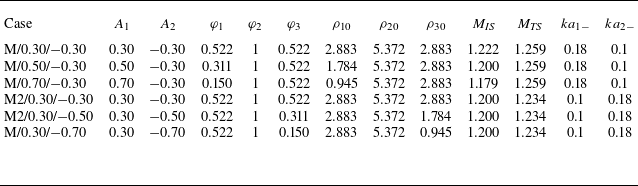
are fixed at 40 and 10 mm, respectively. To control RMI at the DI, we set
 $ka_{1-}=$
0.18 and
 $ka_{2-}=$
0.1 with constant
 $A_2=0.3$
and
 $M_{\textit{TS}}=$
1.259. For the UI perturbation manipulation,
 $ka_{1-}=$
0.1 and
 $ka_{2-}=$
0.18 with fixed
 $A_1=$
0.3 and
 $M_{\textit{IS}}=$
1.20. Figure 13 shows theoretical predictions from (3.21)–(3.22) for
 $\dot {a}_2$
versus
 $A_1$
(red line) and (3.31)–(3.32) for
 $\dot {a}_1$
versus
 $A_2$
(black line). Null growth rates indicate perturbation freeze-out at the interface (Mikaelian Reference Mikaelian1985). Six numerical simulations (symbols in figure 13) with initial parameters appearing in table 6 validate this approach, with two distinct configurations achieving freeze-out at either the UI or DI. The cases for modulating the perturbation growth at the DI (UI) via changing the Atwood number of the UI (DI) are named ‘M/
 $A_1$
/
 $A_2$
’ (‘M/
 $A_1$
/
 $A_2$
’).
Initial conditions of the simulations designed to realize manipulation of perturbation growth at either the UI or DI. The symbols have the same meaning as those in tables above.

The schlieren images for all six cases are presented in figure 14. Figure 14(a–c) show the DI modulation by varying
 $A_1$
. When
 $A_1=$
0.3, the DI undergoes phase reversal analogous to a shocked single heavy–light interface. When
 $A_1=$
0.5, the DI amplitude stagnates (almost from 53-1613
 $\unicode {x03BC}$
s). When
 $A_1=$
0.7, the UI grows substantially, while the DI evolves in phase-synchronization with the UI. Figure 14(d–f) demonstrate the UI modulation via
 $A_2$
adjustment. The UI amplitude undergoes amplification when
 $A_2=$
0.3 and remains quasistationary when
 $A_2=$
0.5. When
 $A_2=$
0.7, the basic mode at the UI evolves to the opposite phase with the initial perturbation, synchronizing with the DI evolution.
Schlieren images of interface evolution and wave patterns for (a) case M/0.30/
 $-$
0.30, (b) case M/0.50/
 $-$
0.30, (c) case M/0.70/
 $-$
0.30, (d) case M2/0.30/
 $-$
0.30, (e) case M2/0.30/
 $-$
0.50 and ( f) case M2/0.30/
 $-$
0.70.

Figure 15 presents temporal evolution of fundamental mode amplitudes at the DI (UI) extracted via FFT from simulations with fixed
 $A_2$
(
 $A_1$
). Quantitative results demonstrate controllable modulation of perturbation growth at either interface through Atwood number variation at the opposite interface. Optimized Atwood-number selection achieves perturbation freeze-out at both the UI and DI. Theoretical predictions from (3.21)–(3.22) (lines in figure 15
a) and (3.31)–(3.32) (lines in figure 15
b) show agreement with numerical results (symbols). This validates the analytical framework in § 3.3 for accurately predicting the UI and DI modulation under varying Atwood-number conditions.
A comparison between the processes of modulating RMI under total-transmission and non-total-transmission conditions (§§ 3.2 and 3.4) reveals that the presence of zero-order reverberating waves significantly complicates the development of an analytical dimensionless model for RMI manipulation in a layered system. The total-transmission condition enables the derivation of (3.16)–(3.17), which clearly identify the dimensionless parameters governing RMI modulation at a layer. In contrast, when reverberating waves are present, it becomes considerably more challenging to theoretically derive explicit dimensionless parameters that determine the possible regimes of multi-interface RMI manipulation. Nevertheless, the Atwood numbers of the two interfaces (
 $A_1$
and
 $A_2$
) remain the key dimensionless parameters governing the modulation of multi-interface RMI, regardless of whether total-transmission conditions are met.
Comparison of the basic-mode amplitudes of the UI (
 $a_1$
) and the DI (
 $a_2$
) from simulations (symbols) with those predicted by models (lines) for the cases designed to manipulate RMI at the DI (a) and the cases aiming to control perturbation growth at the UI (b).

4. Conclusions
The Atwood-number dependence in a shock-accelerated heavy fluid layer is systematically examined through theoretical modelling and numerical simulations. To isolate the intrinsic interface-coupling effect, reverberating waves are eliminated by imposing a total-transmission condition at the DI. Variation of the UI Atwood number,
 $A_1$
, reveals a strong influence on the morphological evolution of both interfaces. Specifically, an unexpected phase inversion is observed at the UI under low-
 $A_1$
conditions. As
 $A_1$
increases, the perturbation evolution at the DI progressively synchronizes in phase with that at the UI, indicating a strengthening of the UI-driven coupling. Phase inversion at the DI is absent under high-
 $A_1$
conditions. A comprehensive theoretical framework, incorporating startup, linear and nonlinear stages, is developed and validated to quantify the UI–DI coupling effect across a wide range of Atwood numbers.
Based on the established theory, we derive dimensionless formulae that define the modulation of multi-interface RMI under the total-transmission condition. Theoretical derivation first identifies four governing dimensionless parameters: the Atwood numbers of the UI and DI (
 $A_1$
and
 $A_2$
), the dimensionless layer width, and the postshock amplitude ratio. The theory further proves that, in the absence of reverberating waves, it is theoretically impossible to simultaneously freeze perturbation growth at both interfaces by adjusting only the Atwood numbers. Eight distinct regimes of modulation achievable by varying
 $A_1$
and
 $A_2$
are identified and validated through numerical simulations. Moreover, the model applies to both in-phase and antiphase initial perturbations at the interfaces.
Subsequently, we systematically change both
 $A_1$
and
 $A_2$
to investigate the perturbation evolution in a shocked fluid layer with reverberating waves. The influence of
 $A_1$
on perturbation growth is found to be similar to that in scenarios without reverberations. When
 $A_2$
is increased while
 $A_1$
is held constant, the enhanced interface-coupling effect is counterbalanced by stronger rarefaction waves inside the layer. As a result, the amplitude growth rate at the UI remains largely insensitive to changes in
 $A_2$
. In contrast, the growth of the DI amplitude shows a clear positive correlation with
 $A_2$
. A theoretical model that incorporates both the interface-coupling effect and reverberating waves is derived, quantifying the dependence of linear perturbation growth on the Atwood numbers in a shocked heavy layer. Importantly, the results show that under high-
 $A_2$
conditions, accurate prediction of amplitude evolution at both the UI and DI requires the consideration of more than four reverberating waves within the layer.
Finally, we investigate the manipulation of instability in a shock-accelerated heavy layer with reverberating waves. Guided by the proposed theory, we strategically configure
 $A_1$
and
 $A_2$
to achieve targeted control over instability growth. This approach allows for the independent modulation of perturbation growth at the DI for a fixed
 $A_2$
, and at the UI for a fixed
 $A_1$
. Simulations confirm these theoretical predictions, successfully demonstrating distinct modulation scenarios at each interface. Crucially, this study establishes that instability growth at one interface can be controlled by adjusting the Atwood number of the opposite interface, irrespective of the presence of reverberating waves.
These findings enhance the fundamental understanding of instability manipulation in shocked fluid layers. Moreover, they suggest a potential application in ICF: by strategically choosing ablator materials to adjust the interface Atwood numbers inside the capsule, hydrodynamic instabilities during ignition could be effectively suppressed. While the current work concentrates on the interaction of a fluid layer with a weak shock, future studies will employ compressible theories to examine how modulation of instability depends on the Atwood number under strong shock conditions. The resulting compressible models for multi-interface RMI need to fully account for how acoustic waves, induced by shock–interface interactions, influence perturbation evolution. It should also be noted that the present investigation deals exclusively with perturbation growth at successive interfaces between gaseous media. Subsequent research will extend this analysis to include the effects of material properties such as elasticity and viscosity, with the goal of exploring instabilities at interfaces involving solid and liquid, conditions frequently encountered in ICF capsules.
Funding
This work was supported by the National Natural Science Foundation of China (nos. 123B2034, 12372281 and 12388101) and the Strategic Priority Research Program of Chinese Academy of Sciences (no. XDB0620201).
Declaration of interests
The authors report no conflict of interest.