1. INTRODUCTION
Effective navigation of Mars probes is essential to successfully implement Mars missions. Traditional spacecraft navigation has been primarily achieved by means of Earth-based observations such as radio tracking range and range-rate (Doppler) measurements from the Deep-Space Network (DSN) and Delta-Differential One-way Ranging (Delta-DOR) measurements from Very-Long-Baseline Interferometry (VLBI). Despite its success, one of the inherent drawbacks of Earth-based navigation is that the communication may be interrupted when the Sun or a planet are lying in the line connecting the Earth and the probe. Another drawback is that the communication time delay caused by round-trip light time is rather long. For Mars missions, the round-trip delay is more than forty minutes.
Autonomous navigation, using on board spacecraft computers, is an attractive way to overcome these drawbacks and reduce the dependence on Earth-based tracking stations. Several different measurement methods for autonomous navigation have been proposed through different measurement types (Chory et al., Reference Chory, Homan and LeMay1986; Hicks and Wiesel, Reference Hicks and Wiesel1992; Psiaki, Reference Psiaki1999; Christian and Lightsey, Reference Christian and Lightsey2010; Ma et al., Reference Ma, Fang and Ning2013).
Optical measurement autonomous navigation has been an attractive research focus in space missions. Many methods have been proposed in recent years (Chausson and Delavault, Reference Chausson and Delavault2003; Stastny and Gellert, Reference Stastny and Gellert2008; Paluszek et al., Reference Paluszek, Mueller and Littman2010). The first successful attempt at fully automated navigation is the Deep Space 1 mission using the images of asteroids (Bhaskaran et al., Reference Bhaskaran, Riedel, Synnott and Wang2000). In January 2004, during the flyby of comet Wild-2, the STARDUST mission used the images of the comet to improve the state information. In this mission, the line of sight of the comet was used as observation data (Bhaskaran et al., Reference Bhaskaran, Desai, Dumont, Kennedy, Null, Owen, Riedel, Synnott and Werner1998). Subsequently, another successful application of the optical autonomous navigation was accomplished by the Deep Impact mission (Mastrodemos et al., Reference Mastrodemos, Kubitschek and Synnott2005).
Phobos and Deimos, the two natural moons of Mars, are important optical navigation information sources available for Mars missions, and a method was proposed by Duxbury et al. (Reference Duxbury, Born and Jerath1974) to navigate Mariner 9. However, during the phase when the probe orbits near to Mars, the ephemeris bias of Martian moons are crucial to navigation accuracy. The ephemeris accuracy of the two Martian moons may be no better than several kilometres (Lainey et al., Reference Lainey, Dehant and Patzold2007). Moreover, Phobos is an irregular body with size of 13·4 × 11·2 × 9·2 km (Deimos is 7·8 × 6·0 × 5·1 km). Because of their irregular shape and the different phase angle of sun light, the difference between the barycentre and the centre of brightness of the Martian moons is considerable. So, the Martian moons' apparent position error may be several kilometres or more, which could result in about 0·1° angle observation error when the range between the probe and the moon is 5000 km. Therefore it is very difficult to attain high navigation accuracy by using on board images of Phobos and Deimos alone during the phase orbiting Mars. Especially for low Mars orbits, optical autonomous navigation by viewing Martian moons is very difficult due to the dynamics model error and the low accuracy measurements that can be obtained.
On the other hand, radiometric measurement is generally used in spacecraft tracking due to its high accuracy and convenience. The Satellite-to-Satellite Tracking observation (SST) including radiometric range and range-rate (Doppler) measurements has been used for navigation by orbit determination. For example, a spacecraft can be tracked from the ground while it is tracking another satellite. Combining the observations, one can successfully estimate the orbits of both satellites. This method is used to determine the orbits of spacecraft in low Earth orbit with Tracking Data Relay Satellite Systems (TDRSS) and the Global Positioning System (GPS). For autonomous navigation on a Mars mission, a Mars Network based on Satellite-to-Satellite radiometric tracking can be used (Lightsey et al., Reference Lightsey, Mogensen, Burkhart, Ely and Duncan2008). It is designed to aid Mars approach and Entry/Descent/Landing (EDL) navigation. Another SST method is called linked, autonomous, interplanetary satellite orbit of two or more spacecraft. This method requires that at least one of the satellites is in an orbit with a unique size, shape and orientation, such as spacecraft in halo orbit or at Sun-Earth L1 and L2 points (Hill and Born, Reference Hill and Born2007; Mark and Psiaki, Reference Mark and Psiaki2011). However, it has been proved that in a two-body problem, SST cannot be used alone to estimate the absolute positions of the spacecraft involved, because it suffers the rank defect problem of Jacobian matrix in these circumstances (Liu and Liu, Reference Liu and Liu2001). During the Mars orbit phase, the system dynamics model is close to a two-body problem, so SST cannot be used alone to implement navigation.
In order to improve the Mars probe autonomous navigation accuracy during the Mars orbit phase, we propose a new autonomous navigation method which requires estimating two probes' orbits simultaneously with combining SST range and range-rate measurements by two probes that are orbiting Mars and optical measurement of the images of Martian moons from one probe. High accuracy of the optical measurement is not necessary. The research shows that the method can successfully realise autonomous navigation during the Mars orbit phase. In particular, for the case of one probe in low orbit and another in high orbit equipped with on board optical measurement, high navigation accuracy can be obtained, even if the low orbit probe's dynamics model error is considerable.
2. SCENARIO AND VISIBILITY
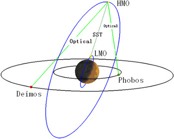
In a future Mars mission, it could be designed that two probes are launched together. After entering the Mars orbit phase, one probe enters Low Mars Orbit (LMO) to explore Mars, and another enters High Mars Orbit (HMO) to relay communications to the Earth and view Phobos and Deimos for navigation. The SST radio range and range-rate measurements between LMO and HMO can be easily obtained and need very short communication time. It does not require LMO optical measurement to view Phobos and Deimos. With SST data and optical measurement of HMO, the two probes' autonomous navigation can be performed simultaneously. The goal is to determine the combined satellite state vector without any supplemental ground tracking. The states of the two spacecraft should be estimated altogether. Figure 1 shows orbits and measurements of the two probes and Martian moons in the scenario.
The scenario of SST and Martian Moons optical measurement navigation.

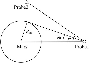
The scenario requires analysing the visibility of SST between LMO and HMO and optical measurement from the probe to Phobos and Deimos. If LMO and HMO are not obstructed in line by Mars, the visibility condition of SST is satisfied.
In Figure 2, R m is the radius of Mars, r1 and r2 are the position vector of probe-1 and probe-2 in Mars centre coordinate system. ψ is the angle between the vector from probe-2 to probe-1 and from Mars centre to probe-1. The visibility condition is
1) ψ > ψ 0
2)
 $\Vert {{\bi r}_{\rm 2} - {\bi r}} \Vert \lt \sqrt {\Vert {{\bi r}_{\rm 1}} \Vert^2 - R_{\rm m}^2} $, if ψ < ψ 0

The visibility of SST.

As for optical measurement, there are four factors that determine whether the probe could observe Martian moons: (1) the probe and Martian moons are not obstructed in line by Mars; (2) Martian moons are not in the shadow of Mars; (3) Martian moons must reflect enough solar light to the probe; and (4) the sun and Mars are out of the field of view of the navigation optical sensor.
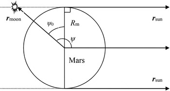
Analysis as to whether the probe and Martian moon are obstructed in line by Mars is similar to that of SST tracking. Figure 3 shows whether a Martian moon is in the shadow of Mars. Rm is the radius of Mars; rsun is the position vector of the sun, and rmoon is the position vector of a Martian moon. Then, ψ is the angle between rmoon and rsun, and  $\psi _0 = \arcsin ({{R_{\rm m}} / {\Vert {{\bi r}_{{\rm moon}}} \Vert}})$. If ψ > ψ 0, the Martian moon is not in the shadow of Mars.
Geometry of Mars shadow.

Whether Martian moons reflect enough solar light to the probe depends on the phase angle ψ from Martian moon to the sun and to the probe, here,
 $$\psi = \arccos \left[\displaystyle{{({\bi r}_{{\rm sun}} - {\bi r}_{{\rm moon}} ) \cdot ({\bi r} - {\bi r}_{{\rm moon}} )} \over {\Vert {{\bi r}_{{\rm sun}} - {\bi r}_{{\rm moon}}} \Vert\Vert {{\bi r} - {\bi r}_{{\rm moon}}} \Vert}}\right]$$
where, r is the position vector of the probe. If ψ exceeds 30°, it is considered that the Martian moon can reflect enough solar light to the probe.
If the angle between the vector of the Sun or Mars and the vector of Martian moons to the probe exceeds the maximum angle of field of view, it is thought that the Sun or Mars are out of view of the navigation optical sensor.
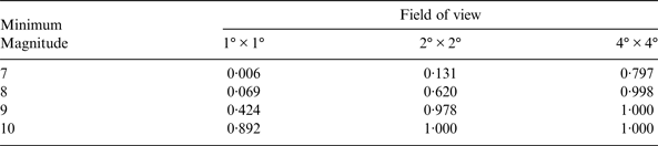
In addition, for optical measurement, at least three stars with sufficient brightness in the same field of view as a moon of Mars are required. As the orbital motion of the probe and Martian moon, a moon of Mars may be in all possible orientations of the celestial sphere in the field of view of the probe. In order to analyse the likelihood of at least three stars with sufficient brightness being in the same field of view, we divide the celestial sphere into 360 × 180 grids by the direction with interval of 1° from 0° to 360° in right ascension and from −90° to 90° in declination.
Table 1 shows the probability of the grids with at least three stars in the same field of view, which is based on Hipparcos-Tycho catalogue (Hog et al., Reference Hog, Fabricius, Makarov, Urban, Corbin, Wycoff, Bastian, Schwekendiek and Wicenec2000). The cases of different sufficient stellar brightness and different fields of view are given respectively.
The probability with at least three stars in the same view.
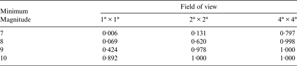
The suitable field of view and the capability of viewing minimum stellar magnitude for a probe can be selected according to Table 1.
3. AUTONOMOUS NAVIGATION ALGORITHM
3.1. System Dynamics
During the Mars orbit phase, the probe dynamics should be established in the J2000·0 Mars-centre Mars centre equator inertial coordinate system. The dynamic model can be written as
 $$ \ddot{\bi r} = {\bi a}_0 + {\bi a}_{ns} + {\bi a}_{nbody} + {\bi a}_{srp} + {\bi a}_{drag} + {\bi a}_\varepsilon $$
For Mars probe, besides the Mars body centre gravitational force a0, other perturbation forces include the Mars non-spherical gravitational force ans, the third body gravitational perturbations from the Sun and other major planets anbody, the solar radiation pressure asrp. Atmosphere drag adrag should also be considered for very low orbit, which is given in the Appendix. In addition, aε is other much smaller force acting on the spacecraft that can be ignored, such as gravitational forces of Martian moons. The RKF7(8) algorithm is applied for the orbit propagation of this dynamic model.
Because the on board computer has limited capacity, the on board dynamic navigation model must be simplified. In order to analyse how the model errors affect navigation precision, a precise dynamic model (model-1) is set as a criterion and a simplified model (model-2) is used for state estimation for on board navigation, as shown in Table 2.
Different options of precise dynamics model and simplified model.

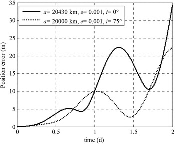
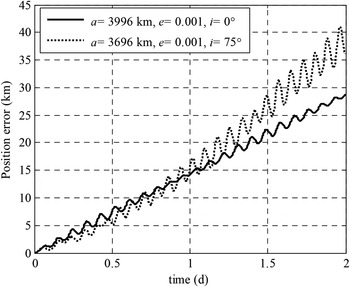
In order to analyse the propagating errors of the simplified model, there are four different orbits being propagated for two days, which are LMO with low-inclination (a = 3996 km, e = 0·001, i = 0°), LMO with high-inclination (a = 3696 km, e = 0·001, i = 75°), HMO with low-inclination (a = 20430 km, e = 0·001, i = 0°) and HMO with high-inclination (a = 20000 km, e = 0·001, i = 75°).
The position difference between model-1 and model-2 is compared in Figure 4 and Figure 5. The figures show that the position errors due to dynamics model error of HMO are several tens of metres for two days' propagation. As to LMO, the position error for two days' propagation is several tens of kilometres.
HMO propagation difference between simplified model and precise model.

LMO propagation difference between simplified model and precise model.

3.2. Measurement models.
3.2.1. Optical measurement
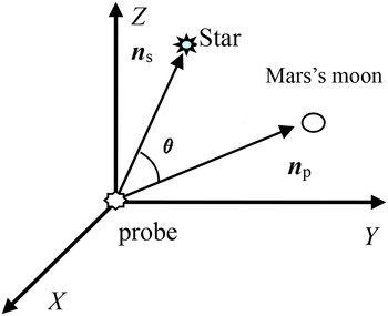
An image photo of the probe on board optical sensor is sketched in Figure 6. The angle θ = arcos(ns·np) is the angle between ns and np, where, ns is the line-of-sight vector from the probe to the background star in the probe centre inertial coordinate system, and np is that of the Mars moon. These vectors are in the probe centre inertial coordinate system.
Optical measurement of Martian moon and background star.

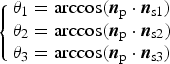
If there are three background stars and a Martian moon in image, then the image should have three angles (θ 1,θ 2,θ 3) between the Martian moon and the three background stars. The position unit vectors of the three background stars (ns1, ns2, n s3) can be obtained from the Tycho-2 star catalogue. According to the angles (θ 1,θ 2,θ 3) and the unit vectors (ns1, ns2, n s3), the unit vector np is obtained as
 $$\left\{\matrix{\theta _1 = \arccos ({\bi n}_{\rm p} \cdot {\bi n}_{{\rm s1}}) \cr \theta_2 = \arccos ({\bi n}_{\rm p} \cdot {\bi n}_{{\rm s2}}) \cr \theta _3 = \arccos ({\bi n}_{\rm p} \cdot {\bi n}_{{\rm s3}} )} \right. $$
If there are more than three background stars in image, the least square algorithm can be used. In the probe centre inertial coordinate system, np(x np, y np, z np) is the unit vector of the Martian moon, the measurement data right ascension α and declination δ can be obtained.
 $$\alpha = \arctan \left(\displaystyle{{y_{{\rm np}}} \over {x_{{\rm np}}}} \right),\quad\delta = \arcsin \left(\displaystyle{{z_{{\rm np}}} \over {r_{{\rm np}}}} \right)$$
In the Mars centre inertial coordinate system, r(x, y, z) is the position vector of probe, and rm(x m, y m, z m) is the Martian moon position vector. Then, rp(x p, y p, z p) = rm – r is the position vector of the Martian moon in the probe centre inertial coordinate system, the measurement model right ascension α and declination δ are obtained:
 $$\alpha = \arctan \left(\displaystyle{{y_{\rm p}} \over {x_{\rm p}}} \right),\quad\delta = \arcsin \left(\displaystyle{{z_{\rm p}} \over {r_{\rm p}}} \right)$$
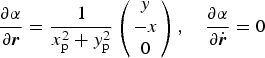
The partial derivative of right ascension α and declination δ for state variables are as follows,
 $$\displaystyle{\partial \alpha \over \partial {\bi r}} = \displaystyle{1 \over x_{\rm p}^2 + y_{\rm p}^2} \left(\matrix{y \cr - x \cr 0} \right), \quad \displaystyle{\partial \alpha \over \partial \dot{\bi r}} = 0$$
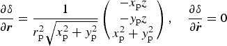 $$\displaystyle{{\partial \delta} \over {\partial {\bi r}}} = \displaystyle{1 \over {r_{\rm p}^2 \sqrt {x_{\rm p}^2 + y_{\rm p}^2}}} \left( \matrix{ - x_{\rm p} z \cr - y_{\rm p} z \cr x_{\rm p}^2 + y_{\rm p}^2 } \right),\quad\displaystyle{{\partial \delta} \over {\partial \dot{\bi r}}} = 0$$
3.2.2. Range measurement and Doppler measurement
There are two probes orbiting Mars, and the first probe position and velocity vectors are  ${\bi r}_1 (x_1, y_1, z_1 )$, and
 $ \dot{\bi r}_1 (\dot x_1, \dot y_1, \dot z_1 )$, and those of the second probe are r2(x 2, y 2, z 2), and
 $ \dot{\bi r}_2 (\dot x_2, \dot y_2, \dot z_2 )$.
Then, the models of range measurement ρ and Doppler measurement  $\dot \rho $ are expressed
 $$\rho = \Vert {{\bi r}_1 - {\bi r}_2} \Vert = \sqrt {(x_1 - x_2 )^2 + (y_1 - y_2 )^2 + (z_1 - z_2 )^2} $$
 $$\dot \rho = \displaystyle{{({\bi r}_1 - {\bi r}_2 ) \cdot ( \dot{\bi r}_1 - \dot{\bi r}_2 )} \over \rho} = \displaystyle{{(x_1 - x_2 )(\dot x_1 - \dot x_2 ) + (y_1 - y_2 )(\dot y_1 - \dot y_2 ) + (z_1 - z_2 )(\dot z_1 - \dot z_2 )} \over {\sqrt {(x_1 - x_2 )^2 + (y_1 - y_2 )^2 + (z_1 - z_2 )^2}}} $$
The partial derivative of range measurement ρ and Doppler measurement  $\dot \rho $ for state variables are computed as follows,
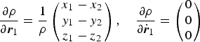 $$\displaystyle{{\partial \rho} \over {\partial {\bi r}_1}} = \displaystyle{1 \over \rho} \left( \matrix{x_1 - x_2 \cr y_1 - y_2 \cr z_1 - z_2 } \right),\quad\displaystyle{{\partial \rho} \over {\partial \dot{\bi r}_1}} = \left( \matrix{0 \cr 0 \cr 0} \right)$$
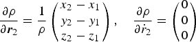 $$\displaystyle{{\partial \rho} \over {\partial {\bi r}_2}} = \displaystyle{1 \over \rho} \left( \matrix{x_2 - x_1 \cr y_2 - y_1 \cr z_2 - z_1 } \right),\quad\displaystyle{{\partial \rho} \over {\partial \dot r_2}} = \left( \matrix{0 \cr 0 \cr 0 } \right)$$
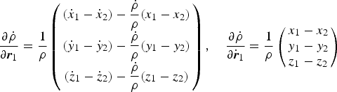 $$\displaystyle{{\partial \dot \rho} \over {\partial {\bi r}_1}} = \displaystyle{1 \over \rho} \left( \matrix{(\dot x_1 - \dot x_2 ) - \displaystyle{{\dot \rho} \over \rho} (x_1 - x_2 ) \cr (\dot y_1 - \dot y_2 ) - \displaystyle{{\dot \rho} \over \rho} (y_1 - y_2 ) \cr (\dot z_1 - \dot z_2 ) - \displaystyle{{\dot \rho} \over \rho} (z_1 - z_2 )} \right),\quad\displaystyle{{\partial \dot \rho} \over {\partial \dot{\bi r}_1}} = \displaystyle{1 \over \rho} \left( \matrix{x_1 - x_2 \cr y_1 - y_2 \cr z_1 - z_2} \right)$$
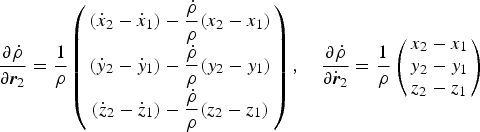 $$\displaystyle{{\partial \dot \rho} \over {\partial {\bi r}_2}} = \displaystyle{1 \over \rho} \left( \matrix{(\dot x_2 - \dot x_1 ) - \displaystyle{{\dot \rho} \over \rho} (x_2 - x_1 ) \cr (\dot y_2 - \dot y_1 ) - \displaystyle{{\dot \rho} \over \rho} (y_2 - y_1 ) \cr (\dot z_2 - \dot z_1 ) - \displaystyle{{\dot \rho} \over \rho} (z_2 - z_1 )} \right),\quad\displaystyle{{\partial \dot \rho} \over {\partial \dot{\bi r}_2}} = \displaystyle{1 \over \rho} \left( \matrix{x_2 - x_1 \cr y_2 - y_1 \cr z_2 - z_1} \right)$$
3.3. Estimation methods
Generally, there are two types of estimation methods used in space navigation. One is the batch method, typically weighted least squares algorithms; the other is sequential processing algorithms including the Extended Kalman Filter (EKF), Unscented Kalman Filter (UKF) and so on. Usually, the batch estimation method is not used for on board estimation because it requires that all measurements to be considered are available before a priori information can be improved. So, the sequential processing algorithm including EKF and UKF is selected to be applied and compared in this paper.
The positions and velocities of the two probes must be estimated altogether to fulfil the requirement of SST radio range and range-rate measurement.
So the state variables include the first probe's position vector r1, velocity vector  $\dot {\bi r}_1 $ and the second probe's position vector r2 and velocity vector
 $\dot {\bi r}_2 $. The state equation and measurement equation are
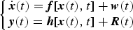 $$\left\{ \matrix{ \dot{\bi x}(t) = {\bi f}[{\bi x}(t),t] + {\bi w}(t) \cr {\bi y}(t) = {\bi h}[{\bi x}(t),t] + {\bi R}(t)} \right.$$
where  ${\bi x}(r_1, \dot r_1, r_2, \dot r_2 )$ is the state parameter, y is measurement consisting of (α, δ) or
 $(\rho, \dot \rho )$, w is the model noise, and R is the measurement noise.
At time t k, xk is the a priori state value, and Pk is the a priori covariance matrix. If at time t k+1, new measurement data yk+1 are obtained, we calculate the estimated value xk+1 at t k+1. After linearization, Equation (13) is written as
 $$\left\{ \matrix{{\bi x}_{k + 1} = {\bf \Phi} \left( {t_{k + 1}, t_k} \right){\bi x}_k + {\bi w}_k \hfill \cr {\bi y}_k {\bi = H}_k {\bi x}_k + {\bi R}_k } \right.$$
Φ(t k+1, t k) is the state transition matrix, and can be found by
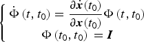 $$\left\{ \matrix{{\dot{\bf \Phi}} \left( {t,t_0} \right) = \displaystyle{{\partial \dot{\bi x}(t_0 )} \over {\partial {\bi x}(t_0 )}}{\bf \Phi} \left( {t,t_0} \right) \hfill \cr {\bf \Phi} \left( {t_0, t_0} \right){\bi \;= I}} \right.$$
The approximate method to calculate Φ(t k+1, tk) is
 $${\bf \Phi} \left( {t_{k + 1}, t_k} \right)= {\bi I} + {\bi F} \vert_{x_{{k + 1} \vert k}} (t_{k + 1} - t_k ) + \displaystyle{1 \over 2}{\bi F}^2 \vert_{x_{ {k + 1} \vert k}} (t_{k + 1} - t_k )^2 $$
where I is a 12 × 12 unit matrix in this system, and F is the Jacobi matrix of dynamics equation. F can be written as
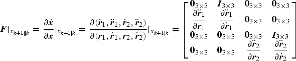 $$ {\bi F} \vert_{x_{ {k + 1} \Vert k}} = {\displaystyle{{\partial \dot{\bi x}} \over {\partial {\bi x}}}} \vert_{x_{ {k + 1} \vert k}} = {\displaystyle{{\partial ( \dot{\bi r}_1, \ddot{\bi r}_1, \dot{\bi r}_2, \ddot{\bi r}_2 )} \over {\partial ({\bi r}_1, \dot{\bi r}_1, {\bi r}_2, \dot{\bi r}_2 )}}} \vert_{x_{ {k + 1} \vert k}} = \left[ {\matrix{ {{\bf 0}_{3 \times 3}} & {{\bi I}_{3 \times 3}} & {{\bf 0}_{3 \times 3}} & {{\bf 0}_{3 \times 3}} \cr {\displaystyle{{\partial \ddot{\bi r}_1} \over {\partial {\bi r}_1}}} & {\displaystyle{{\partial \ddot{\bi r}_1} \over {\partial \dot{\bi r}_1}}} & {{\bf 0}_{3 \times 3}} & {{\bf 0}_{3 \times 3}} \cr {{\bf 0}_{3 \times 3}} & {{\bf 0}_{3 \times 3}} & {{\bf 0}_{3 \times 3}} & {{\bi I}_{3 \times 3}} \cr {{\bf 0}_{3 \times 3}} & {{\bf 0}_{3 \times 3}} & {\displaystyle{{\partial \ddot{\bi r}_2} \over {\partial {\bi r}_2}}} & {\displaystyle{{\partial \ddot{\bi r}_2} \over {\partial \dot{\bi r}_2}}} \cr}} \right]$$
One can refer to the pioneering work of Kalman (Reference Kalman1960) and Kalman and Bucy (Reference Kalman and Bucy1961) for EKF.
A brief process for using the EKF is given here:
1. The propagation of the estimated state from t k to t k+1, is subject to the dynamics model Equation (1), and
${\bar{\bi x}}_{k + 1} $ is the predicted state.2.
${\bar{\bi P}}_{k + 1}$ is the predicted covariance matrix, updated by
(18)$${\bar{\bi P}}_{k + 1} = {\bf \Phi} \left( {t_{k + 1}, t_k} \right){\bi P}_{\bi k} {\bf \Phi} ^{\rm T} \left( {t_{k + 1}, t_k} \right) + {\bi w}_k $$3. Calculate the Kalman gain matrix through
(19)$${\bi K}_{k + 1} = {\bar{\bi P}}_{k + 1} {\bi H}_{k + 1}^{\rm T} [{\bi H}_{k + 1}^{} {\bar{\bi P}}_{k + 1} {\bi H}_{k + 1}^{\rm T} + {\bi R}]^{ - 1} $$4. Update the estimated state through
(20)$${\bi x}_{k + 1} = {\bar{\bi x}}_{k + 1} + {\bi K}_{k + 1} [{\bi y}_{k + 1} - {\bi H}_{k + 1} {\bar{\bi x}}_{k + 1} ]$$5. Update the covariance matrix by
(21)$${\bi P}_{k + 1} = [{\bi I} - {\bi K}_{k + 1} {\bi H}_{k + 1} ]{\bar{\bi P}}_{k + 1} $$






The UKF is a new filtering algorithm for non-linear systems invented by Julier and Uhlmann (Reference Julier and Uhlmann1997). The state transition matrix and the Jacobi matrices of the dynamic equations and observation equations, necessary in EKF, are not required in UKF. The key point of the UKF is based on an Unscented Transformation (UT) that uses a set of appropriately chosen weighted points to parameterise the mean and covariance of the probability distributions. A detailed description of the UKF theory can be found in Julier and Uhlmann (Reference Julier and Uhlmann2004).
A brief process for using the UKF is given here:
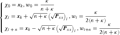
1. Create the set of sigma points by UT as follows
(22)$$\left\{ \matrix{{\bi \chi} _0 = {\bi x}_k, w_0 = \displaystyle{\kappa \over {n + \kappa}} \hfill \cr {\bf \chi} _i = {\bi x}_k + \sqrt {n + \kappa} \left( {\sqrt {{\bi P}_{xx}}} \right)_i, w_i = \displaystyle{\kappa \over {2(n + \kappa )}} \hfill \cr {\bi \chi} _{i \;+\; n} = {\bi x}_k - \sqrt {n + \kappa} \left( {\sqrt {{\bi P}_{xx}}} \right)_i, w_{i + n} = \displaystyle{\kappa \over {2(n + \kappa )}} \hfill} \right.$$where, κ ∈ R, and usually n + κ = 3 when x is assumed to be drawn from Gaussian distribution. In this system, n = 12 and κ = − 9.
- $\left( {\sqrt {{\bi P}_{xx}}} \right)_i $ is the i-th column of the matrix square root of Pxx
w i is the weighted factor associated with the i-th point.
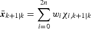
2. The propagation of the estimated state and the covariance matrix
(23)$${\bar{\bi x}}_{k + 1\vert k} = \sum\limits_{i = 0}^{2n} {w_i} {\bi \chi} _{i,k + 1\vert k} $$(24)$${\bi P}_{xx,k + 1\vert k} = \sum\limits_{i = 0}^{2n} {w_i} \left[ {{\bi \chi} _{i,k + 1\vert k} - {\bar{\bi x}}_{k + 1\vert k}} \right]\left[ {{\bi \chi} _{i,k + 1\vert k} - {\bar{\bi x}}_{k + 1\vert k}} \right]^{\rm T} +\; {\bi w}$$3. The prediction of the observation and its covariance matrix are expressed by
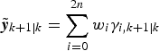
(25)$${\bi \gamma} _{i,k + 1\vert k} = {\bi h}({\bi \chi} _{i,k + 1\vert k} )$$(26)$$\tilde{\bi y}_{k + 1\vert k} = \sum\limits_{i = 0}^{2n} {w_i} {\bi \gamma} _{i,k + 1\vert k} $$(27)$${\bi P}_{yy,k + 1\vert k} = \sum\limits_{i = 0}^{2n} {w_i} \left[ {{\bi \gamma} _{i,k + 1\vert k} - \tilde{\bi y}_{k + 1\vert k}} \right]\left[ {{\bi \gamma} _{i,k + 1\vert k} - \tilde{\bi y}_{k + 1\vert k}} \right]^{\rm T} +\; {\bi R}_{k +1} $$4. Calculate the Kalman gain matrix as follows
(28)$${\bi P}_{xy,k + 1\vert k} = \sum\limits_{i = 0}^{2n} {w_i} \left[ {{\bi \chi} _{i,k + 1\vert k} - {\bar{\bi x}}_{k + 1\vert k}} \right]\left[ {{\bi \gamma} _{i,k + 1\vert k} - \tilde{\bi y}_{k + 1\vert k}} \right]^{\rm T} $$(29)$${\bi K}_{k + 1} = {\bi P}_{xy,k + 1\vert k} \cdot {\bi P}_{yy,k + 1\vert k}^{ - 1} $$5. Update the estimated state and the covariance matrix as follows
(30)$${\bi x}_{k + 1} = {\bar{\bi x}}_{k + 1\vert k} + {\bi K}_{k + 1} \left[ {{\bi y}_{k + 1} - \tilde{\bi y}_{k + 1\vert k}} \right]$$(31)$${\bi P}_{xx,k + 1} = {\bi P}_{xx,k + 1\vert k} - {\bi K}_{k + 1} \cdot {\bi P}_{yy,k + 1\vert k} \cdot {\bi K}_{k + 1}^{\rm T} $$








4. SIMULATION AND RESULTS.
4.1. Scenario Setting
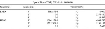
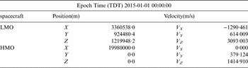
We set two scenarios as samples to substantiate our methods. The first scenario consists of a group of low-inclination orbits of LMO (a = 3996 km, e = 0·001, i = 0°) and HMO (a = 20430 km, e = 0·001, i = 0°). The second scenario consists of high-inclination orbit including LMO (a = 3696 km, e = 0·001, i = 75°) and HMO (a = 20000 km, e = 0·001, i = 75°). Table 3 lists the initial positions and velocities of the low-inclination scenario and Table 4 lists those of the high-inclination scenario in the J2000·0 Mars-equator coordinate System. The effect of probe attitude on visibility is not taken into account in this paper, because the probe can adjust attitude or sensor direction to be adapted to suit the observation.
Orbit parameters of low-inclination scenario.

Orbit parameters of high-inclination scenario.

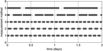
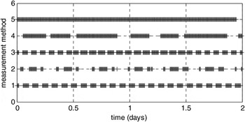
According to the visibility condition in Section 2, Figures 7 and 8 give the visibility of Scenario-1 and Scenario-2, respectively. In these figures, labels 1, 2, 3, 4, and 5 on vertical axis represent SST, optical measurement from LMO to Phobos, optical measurement from LMO to Deimos, optical measurement from HMO to Phobos, and optical measurement from HMO to Deimos, respectively.
The visibility of Scenario-1.

The visibility of Scenario-2.

4.2. Simulation conditions
True data simulation is carried out by propagating the orbit from the initial state under a precise dynamic model (model-1). The true ephemeris is regarded as the criterion for comparison. The simplified dynamics model (model-2) is used for navigation. The difference between the precise and simplified models is taken as model error. The ephemeris of Mars and Martian moons are obtained through JPL's website http://ssd.jpl.nasa.gov/horizons.cgi.
The simulating range measurement error of SST is 10 m (1σ) and the range-rate error of SST is 0·1 m/s (1σ). These simulating measurement errors are in accord with current measurement level and the accuracy can be easily achieved for SST.
To make the measurement error approximate to true measurement condition, the optical measurement error is set according to the following the Equation (32).
 $$\sigma = \sigma _1 + \arctan \Big(\displaystyle{{\sigma _{Eph}} \over {\Delta R}}\Big) + \arctan \Big(\displaystyle{{R_{moon}} \over {\Delta R}}\Big)\sin \displaystyle{\psi \over 2}$$
where σ 1 is the random error with Gaussian distribution of 0·01°, which includes measurement noise and the errors of the stellar location of background stars. σ Eph is Martian moon ephemeris error of 10 km, ΔR is the range from the probe to Martian moon, R moon is the approximate radius of Martian moon of 5 km and ψ is the phase angle from Martian moon to the Sun and the probe.
As the stellar location accuracy of the present stellar catalogue is far higher than 1″ (Hog et al., Reference Hog, Fabricius, Makarov, Urban, Corbin, Wycoff, Bastian, Schwekendiek and Wicenec2000), the effect of stellar location accuracy on navigation accuracy is included in the random error (σ 1) of 0·01°.
In the filter process, the initial position and velocity uncertainty is set as 10 km and 5 m/s respectively for all simulation samples. The initial state covariance and the measurement noise covariance used for navigation filter were as follows:
 $$\displaylines{{\bi P}_0 = diag[(10{\rm \;km)}^2, (10{\rm \;km)}^2, (10{\rm \;km)}^2, (5{\rm \;m/s)}^2, (5{\rm \;m/s)}^2, (5{\rm \;m/s)}^2, \cr (10{\rm \;km)}^2, (10{\rm \;km)}^2, (10{\rm \;km)}^2, (5{\rm \;m/s)}^2, (5{\rm \;m/s)}^2, (5{\rm \;m/s)}^2 ]} $$
 ${\bi R} = diag[(0.1^{\circ} {\rm )}^2, (0.1^{\circ} {\rm )}^2 ]$ for optical data and
 ${\bi R} = diag[(10{\rm \;m)}^2, (0.1{\rm \;m/s)}^2 ]$ for SST data.
4.3. Optical navigation by Viewing to Martian Moons Alone
Theoretically, by using optical measurement alone, LMO and HMO navigation can be performed respectively. In order to analyse the accuracy of the navigation using optical data alone, numerical simulations of autonomous navigation by using only optical data of Martian moons are carried out. The observation data is updated once per 1 minute. The predicted value will be given for navigation during the observation interval.
No matter what the inclination of the orbits, EKF for LMO cannot achieve results. The reason is that the non-linearity of LMO is stronger than that of HMO in the same time span. The results of EKF for LMO by optical measurement alone are divergent due to the inability to acceptably linearize a strongly non-linear system. The reason that the results of UKF for LMO are convergent is due to its properties without linearization. However, the navigation accuracy of UKF is still low, 10 km position error and 8 m/s velocity error in Scenario-1, and 5 km position error and 6 m/s velocity error in Scenario-2.
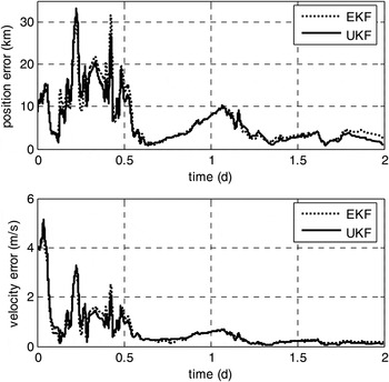
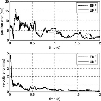
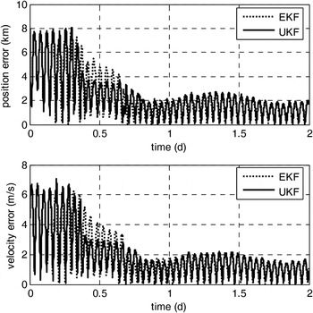
The simulated navigation results of HMO in Scenario-1 are shown in Figure 9 and those in Scenario-2 are shown in Figure 10. The results indicate that autonomous navigation by using optical data alone for HMO, EKF and UKF lead to similar results once converged, and the accuracy of UKF is a little better than that of EKF. The maximum position error is about 10 km and the maximum velocity error is about 0·7 m/s for HMO in Scenario-1, and that in Scenario-2 is 5 km and 0·3 m/s respectively.
Estimate errors of HMO of low-inclination by optical data alone.

Estimate errors of HMO of high inclination by optical data alone.

4.4. Navigation by combining Optical Data and SST Data
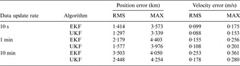
By combining SST data and optical measurement, autonomous navigation of the two probes must be conducted simultaneously. In terms of the given simulation conditions mentioned above, a series of numerical simulations of autonomous navigation by combining optical data of viewing Martian moons and Satellite-to-Satellite radio tracking data are carried out in this section. Similarly, the predicted value will be given for navigation during the observation interval. In order to analyse the navigation performance with different measurement update rate, the measurement date update rate is set to three cases: 10 minutes, 1 minute, and 10 seconds, respectively.
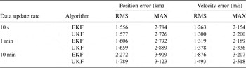
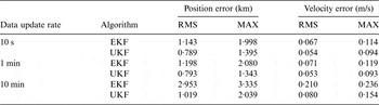
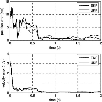
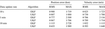
Tables 5 and 6 give the statistical information on the navigation accuracy of Scenario-1 after the filter has converged from the 24th to 48th hour. The simulation navigation results in Scenario-1 with data update rate of 1 minute are shown in Figures 11 and 12.
Estimate errors of LMO in Scenario-1 with 1 minute update rate.

Accuracy comparison of LMO with low inclination.

Accuracy comparison of HMO with low inclination.

In Scenario-1, when the update rate of measurement data is set to be 10 minutes, no matter LMO or HMO, the navigation accuracies by UKF are both better than that of EKF. For LMO, the position and velocity errors of EKF are about 2·2 km of root mean square (RMS) and 1·9 m/s (RMS), respectively. By contrast, those of UKF are 1·8 km and 1·5 m/s, respectively. For HMO, the position and velocity errors of EKF are about 3 km (RMS) and 0·2 m/s (RMS), respectively. By contrast, those of UKF are 1 km and 0·08 m/s, respectively. Especially for HMO, the performance in accuracy of UKF is about three times better than that of EKF.
However, when the update rate of measurement data is set to be either ten seconds or one minute, no matter LMO or HMO, EKF and UKF have similar excellent performance. For LMO, the position errors of both EKF and UKF are about 1·6 km (RMS) and 2·8 km (Maximum), and the velocity errors are about 1·3 m/s (RMS) and 2·2 m/s (Maximum). Meanwhile, for HMO, in the same scenario, the performance in accuracy of UKF is a little better than that of EKF. The position and velocity errors of EKF are about 1·2 km (RMS) and 0·07 m/s (RMS), respectively. By contrast, those of UKF are 0·8 km and 0·05 m/s, respectively.
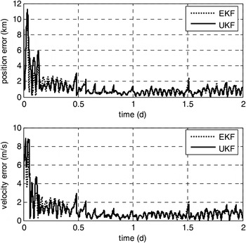
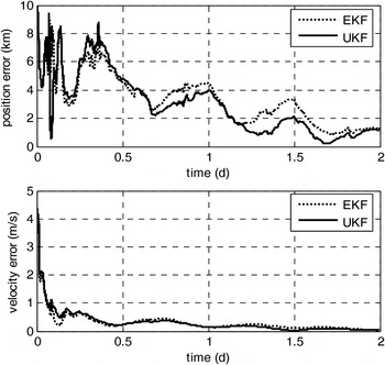
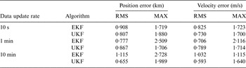
Tables 7 and 8 give statistical information of navigation results of LMO and HMO in Scenario-2 after the filter has converged from the 24th to 48th hour. The simulated navigation results for the cases of LMO and HMO in Scenario-2 of high inclination orbits are shown in Figures 13 and 14.
Estimate errors of HMO in Scenario-1 with 1 minute update rate.

Estimate errors of LMO in Scenario-2 with 1 minute update rate.

Estimate errors of HMO in Scenario-2 with 1 minute update rate.

Accuracy comparison of LMO with high inclination.
Accuracy comparison of HMO with high inclination.

In Scenario-2, with the update rate of measurement data set to be ten minutes, no matter LMO or HMO, the UKF navigation accuracy is also better than that of EKF. For LMO, the position and velocity errors of EKF are about 1·1 km Root Mean Square (RMS) and 1·0 m/s (RMS), respectively. By contrast, those of UKF are 0·65 km and 0·6 m/s, respectively. For HMO, the position and velocity errors of EKF are about 3·5 km (RMS) and 0·25 m/s (RMS), respectively. By contrast, those of UKF are 2·5 km and 0·18 m/s, respectively.
Similarly to Scenario-1, when the update rate of measurement data is set to be either ten seconds or one minute, EKF and UKF have similar excellent performance for LMO. For HMO, the navigation accuracy with data update rate of ten seconds is little better than that of one minute. For LMO, the position errors of both EKF and UKF are about 0·8–0·9 km (RMS) and 1·7–2·0 km (Maximum), and the velocity errors are about 0·7–0·8 m/s (RMS) and 1·7–2·1 m/s (Maximum). Meanwhile, for HMO, in the same scenario, the performance in accuracy of UKF is a little better than that of EKF. For data update rate of one minute, the position and velocity errors of EKF are about 2·2 km (RMS) and 0·15 m/s (RMS), respectively. By contrast, those of UKF are about 1·6 km and 0·1 m/s, respectively.
4.5. Simulation conclusion
From the above simulation results, we conclude that
• No matter whether in Scenario-1 with low inclination orbits or Scenario-2 with high inclination orbits, the autonomous navigation method of Mars probes by combining optical data of viewing Martian moons and Satellite-to-Satellite radio tracking data is practicable.
• EKF and UKF have similar excellent performance with ten seconds and one minute data update rates. Generally, the performance in accuracy of UKF is a little better than that that of EKF. If the measurement data update rate is ten minutes, UKF navigation accuracy is obviously better than EKF. Due to the dynamics model error, the larger the measurement interval is, the more obviously the strong non-linearity occurs. The EKF algorithm requires linearization to the dynamics model but the UKF algorithm does not.
• Because there are 12 state variables in the system, 25 sigma points should be created by UT, and the time consumption of UKF is twenty times more than that of EKF. So EKF performs faster.
• The shorter the measurement data update rate is, the higher the navigation accuracy is. If the measurement data update rate is shorter than one minute, the navigation accuracy is little improved.
• With data update rate less than one minute, for LMO, the autonomous navigation accuracy can attain about 1·6 km (RMS), 2·0–3·0 km (Maximum) in position, and about 1·0 m/s (RMS), 2·0–3·0 m/s (Maximum) in velocity. And for HMO, the autonomous navigation accuracy can attain about 1·5 km (RMS), 3–4 km (Maximum) in position, and about 0·1 m/s (RMS), 0·2 m/s (Maximum) in velocity.
5. CONCLUSION
Aiming at a future Mars programme, this paper presents autonomous navigation of two Mars probes in Low Mars Orbit (LMO) and High Mars Orbit (HMO) by combining optical data of viewing Martian moons and Satellite-to-Satellite radio tracking data during the Mars orbit phase. Visibility analysis, observation data generation, and orbit determination by using EKF and UKF are presented. Then two different scenarios with orbits of low inclination and high inclination are set to evaluate the performance of the two filters.
Results show that when the navigation of Mars probe uses only on board optical images of Martian moons, the maximum position error is 10 km and the velocity error is 0·5–0·7 m/s for HMO. For LMO, the results are divergent. The simulation results indicate that in the scenario of both low and high inclination orbits, the autonomous navigation method of Mars probes by combining optical data of viewing Martian moons and Satellite-to-Satellite radio tracking data is practicable. The autonomous navigation accuracy can always attain position error of about 1–2 km (RMS). Velocity error is about 1 m/s (RMS) for LMO and 0·1 m/s (RMS) for HMO. The performance in accuracy of UKF is a little better than that of EKF, but EKF has a faster computation performance.
ACKNOWLEDGMENTS
This work is supported by the National Natural Science Foundation of China (Grant No.11372150) and the National Basic Research Program of China (973 Program) (2012CB720000).
APPENDIX: SYSTEM DYNAMICS MODEL
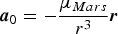 $${\bi a}_0 = - \displaystyle{{\mu _{Mars}} \over {r^3}} {\bi r}$$
 $${\bi a}_{ns} = \displaystyle{{\partial V} \over {\partial {\bi r}}}$$
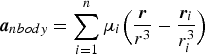 $${\bi a}_{nbody} = \sum\limits_{i = 1}^n {\mu _i} \Big(\displaystyle{{\bi r} \over {r^3}} - \displaystyle{{{\bi r}_i} \over {r_i ^3}} \Big)$$
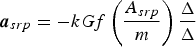 $${\bi a}_{srp} = - kGf\left( {\displaystyle{{A_{srp}} \over m}} \right)\displaystyle{{\bi \Delta} \over \Delta} $$
 $${\bi a}_{drag} = - \displaystyle{1 \over 2}C_D \rho _a \left( {\displaystyle{{A_{drag}} \over m}} \right)V_r {\bi V}_r $$
r is the position vector of the probe,  $r = \Vert {\bi r} \Vert$
 $\mu _{Mars} $ is the gravitational constant of the Mars
 ${\bi r}_i $ is the position vector of the third body including the Sun and other major planets, and
 $r_i = \Vert {{\bi r}_i} \Vert$
 $V$ is the Mars' gravity potential field, and GMM-2B is adopted
 $\mu _i $ is the gravitational constant of the third body such as the Sun and other major planets
 ${\bi \Delta} $ is the position vector of the probe relative to the Sun,
 $\Delta = \Vert {\bi \Delta} \Vert$
 $k$ is the solar radiation pressure coefficient
G is the momentum flux from the Sun at the probe location
f is the eclipse factor, if the probe is in the Mars's shadow f = 0, and if the probe is in sunlight f = 1
 $A_{srp} $ is the probe surface area with solar orientation
 $m$ is the probe mass
 $C_D $ is atmosphere drag coefficient
 $\rho _a $ is the atmosphere density in the position of the probe
 $A_{drag} $ is the probe surface area with drag orientation
 ${\bi V}_r $ is the relative velocity that the probe to atmosphere,
 $V_r = \Vert {{\bi V}_r} \Vert$