1. Introduction
Shock wave/boundary-layer interactions (SBLIs) are critical and fundamental phenomena in the internal and external flows of high-speed vehicles (Babinsky & Harvey Reference Babinsky and Harvey2011). SBLIs in hypersonic flows can induce unexpected heat flux augmentation and directly endanger the structural safety of high-speed vehicles. As a result, aerothermal effects in hypersonic SBLIs have drawn considerable attention. Building on extensive research of canonical two-dimensional (2-D) interactions, recent studies are shifting toward more complex three-dimensional (3-D) interactions that closely represent practical scenarios (Sabnis & Babinsky Reference Sabnis and Babinsky2023; Zuo & Pirozzoli Reference Zuo and Pirozzoli2024). Swept interactions, where the obstacle or shock generator is oriented at an angle to the incoming flow (e.g. swept compression ramps, sharp fins and swept impinging shocks), are a representative category of 3-D SBLIs. These interactions exhibit strong 3-D characteristics featured by the spanwise variations due to sweep effects. Accordingly, a key issue of swept SBLIs has been the pursuit of flow symmetry to achieve a unified collapse of flow field and surface properties, thereby enhancing the understanding of flow mechanisms and informing practical aerodynamic design.
In past years, considerable efforts have been dedicated to studying turbulent swept SBLIs (Settles & Dolling Reference Settles and Dolling1990; Knight, Horstman & Bogdonoff Reference Knight, Horstman and Bogdonoff1992), leading to the identification of two primary symmetry types: cylindrical symmetry and conical symmetry. According to Settles & Teng (Reference Settles and Teng1984), cylindrical symmetry is observed in inviscid attached shock configurations, whereas conical symmetry arises in inviscid detached shock configurations. For practical non-semi-infinite configurations, the presence of inception effects prevents these symmetries from being strictly defined. Instead, they manifest as asymptotic or quasi-symmetries. Furthermore, the conical ‘free interaction’ principle proposed by Settles & Kimmel (Reference Settles and Kimmel1986) provides a framework for correlating flow topologies and surface pressures across geometrically diverse configurations and various flow conditions. Regarding aerothermal effects, Rodi & Dolling (Reference Rodi and Dolling1995) conducted heat transfer measurements on the turbulent swept interaction induced by a sharp fin. The results showed that the heat flux was nearly constant along rays from the virtual conical origin (VCO) of the surface pressure field. They argued that the heat transfer distribution was not strictly conical, as a purely conical flow field would exhibit a
 $1/r$
decay in both heat transfer and skin friction. However, Kim & Settles (Reference Kim and Settles1988) argued that the uniform distribution of skin friction observed along the ray in swept fin interactions would also support the quasi-conical theory. Following their argument, in the present work, we consider the uniform heat flux distribution along the ray to exhibit conical symmetry, consistent with other surface properties such as pressure (Settles & Dolling Reference Settles and Dolling1990) and skin friction coefficient (Kim & Settles Reference Kim and Settles1988). In addition to surface properties, recent research has extended to the quasi-conical scaling of velocity fields (Vanstone et al. Reference Vanstone, Musta, Seckin and Clemens2018; Adler & Gaitonde Reference Adler and Gaitonde2019). Generally, the flow symmetries in turbulent swept SBLIs have been well understood.
As the Mach number increases, the aerothermal challenges in SBLIs become increasingly critical. Moreover, for high-Mach-number vehicles travelling at high altitudes, the transitional SBLIs, characterised by the laminar-to-turbulent transition occurring within or near the interaction zone, are prevalent. However, the aerothermal effects in hypersonic transitional swept SBLIs remain poorly understood. Existing studies on 2-D or axisymmetric transitional interactions demonstrate that the transition to turbulence significantly complicates the flow structures and the corresponding aerothermal effects in SBLIs. Specifically, when the transition occurs downstream of the reattachment, the transition onset is found to move upstream towards the reattachment location with increasing interaction strength, Reynolds number and upstream disturbance (Leidy et al. Reference Leidy, Neel, Tichenor, Bowersox and Schmisseur2021; Davami et al. Reference Davami2024; Benitez et al. Reference Benitez2025). This process is accompanied by an enhancement in heat transfer due to boundary-layer transition. For swept SBLIs, the spanwise variation of Reynolds number (at the inviscid shock) and interaction length supposedly leads to spanwise-varying transition behaviour. However, the specific distribution of the transition onset and its influence on the aerothermal symmetry of swept SBLIs remain unknown.
In addition to boundary-layer transition, sweep effects may also influence the heat flux streak structure. The streaks are commonly observed downstream of reattachment in the transitional SBLIs, causing heat flux fluctuations along the span and significantly enhancing local heat transfer. Various explanations have been proposed for these heat flux streaks. Traditionally, they are regarded as the footprints of Görtler vortices induced by centrifugal forces on the concave surface near reattachment (Benay et al. Reference Benay, Chanetz, Mangin, Vandomme and Perraud2006; Chuvakhov et al. Reference Chuvakhov, Borovoy, Egorov, Radchenko, Olivier and Roghelia2017; Cao, Klioutchnikov & Olivier Reference Cao, Klioutchnikov and Olivier2019). The upwash and downwash effects of these counter-rotating streamwise vortices lead to alternating heat flux variations. More recently, resolvent analysis has identified several convective mechanisms (including the above Görtler instability) that amplify external disturbances to form heat flux streaks in globally stable flows (Dwivedi et al. Reference Dwivedi, Sidharth, Nichols, Candler and Jovanović2019; Lugrin et al. Reference Lugrin, Beneddine, Leclercq, Garnier and Bur2021; Hao et al. Reference Hao, Cao, Guo and Wen2023). Moreover, global stability analysis on several strongly separated flows has revealed that intrinsic instabilities can also induce heat flux streaks (Sidharth et al. Reference GS, Dwivedi, Candler and Nichols2018; Hao et al. Reference Hao, Cao, Wen and Olivier2021). For transitional swept SBLIs, it is unclear as to how the spanwise variation in the interaction zone affects the streaks originating from different mechanisms. The influence of sweep angle also requires further exploration.
Shock–shock interaction is another key feature downstream of reattachment in hypersonic ramp flows, especially for large ramp angles with strong separation and reattachment shocks. These interactions generate waves that impinge on the ramp, causing complex heat flux variations. In 2-D hypersonic ramp flows, type VI shock–shock interactions are commonly encountered (Gonzales, Suzuki & Sakaue Reference Gonzales, Suzuki and Sakaue2020). However, for the swept ramps with the same ramp angle, the inviscid shock tends to detach as the sweep angle increases. Consequently, more complex shock–shock interactions other than type VI may occur, which produce various configurations of heat flux peaks and complicate the aerothermal symmetry. In a relevant study, Ishiguro et al. (Reference Ishiguro, Nagai, Asai and Nakakita2007) have experimentally investigated the influence of angle of attack (AOA) on the heat transfer in a
 $30^\circ$
compression ramp at Mach 10.4. Their results showed that as the AOA was gradually increased from
 $0^\circ$
to
 $20^\circ$
, the shock–shock interaction above the ramp evolved from type VI to type V and finally to type IV, leading to drastic changes in heat flux distribution. However, research regarding this phenomenon is relatively scarce and the understanding remains limited for hypersonic swept ramp flows.
Currently, research efforts in the numerical simulation of 3-D SBLIs still face a dilemma between accuracy and cost. Reynolds-averaged Navier–Stokes simulations struggle to accurately predict heat transfer due to the inherent unsteadiness and three-dimensionality of flows (Leger, Bisek & Poggie Reference Leger, Bisek and Poggie2016). Recent fruitful advancements in high-fidelity simulations have significantly improved the characterisation of fine flow structures and unsteady behaviour (Zhang et al. Reference Zhang, Guo, Dang and Li2022; Gaitonde & Adler Reference Gaitonde and Adler2023), but studies specifically addressing aerothermal effects in these interactions remain scarce. The expensive time and hardware costs limit the application of high-fidelity simulation to explore a wide range of cases or extend simulation durations. In contrast, experiments have been continuously offering reliable data and valuable insights for complex SBLI problems. However, conventional single-point heat flux gauges fall short in capturing complex 3-D aerothermal phenomena, while infrared imaging, despite offering a global perspective, lacks the temporal resolution to capture unsteady phenomena in short-duration hypersonic tests (Smith et al. Reference Smith, Siddiqui, Ledbetter, Gragston, Shine, Ibanez, McGruder and Bowersox2024). Recent advances in fast-responding temperature-sensitive paint (fast TSP) offer new opportunities to comprehensively understand the complex aerothermal issues in hypersonic flows, due to the superior spatial and temporal resolution. For example, fast TSP measurements in the high enthalpy shock tunnel Göttingen (HEG) was first demonstrated on a transition cone by Ozawa et al. (Reference Ozawa, Laurence, Schramm, Wagner and Hannemann2015), followed by applications on other models in the same facility (Risius et al. Reference Risius, Beck, Klein, Henne and Wagner2017; Laurence et al. Reference Laurence, Ozawa, Martinez Schramm, Butler and Hannemann2019). In particular, our previous work has developed a time-resolved heat flux field measurement technique using fast TSP for shock tunnel experiments (Liu et al. Reference Liu, Zhuang, Zhang, Wang, Liu and Peng2024).
Building on this technique, the present study aims to experimentally investigate the complex aerothermal effects in the hypersonic transitional swept SBLIs and explore heat transfer symmetry, a topic that, to the authors’ knowledge, has been rarely reported in literature. The obtained global heat transfer fields on the ramps with various sweep angles reveal intricate aerothermal phenomena driven by 3-D separation, reattachment and transition. After examining the states of upstream and reattached boundary layers, the time-averaged heat transfer characteristics are analysed in terms of the heat flux peaks downstream of reattachment, the heat flux streaks, the low heat transfer region near the swept ramp’s leading side and the spanwise variations in heat transfer beneath the reattached boundary layer. Finally, a local quasi-conical symmetry of heat transfer is identified upstream of reattachment, while this symmetry is disrupted downstream due to spanwise variations in transition onset, shock–shock interaction and heat flux streaks.
2. Experimental set-up
2.1. Wind tunnel and test model
The experiments were conducted in the
 $\varPhi$
0.6m shock tunnel at the Chinese Aerodynamic Research and Development Center. This tunnel simulates Mach 6–12 flows with an effective duration of 2–13 ms. This work used nitrogen as the driven gas. The incoming flow parameters, including Mach number (
 $M_{\infty }$
), total temperature (
 $T_0$
) and pressure (
 $P_0$
), free stream density (
 $\rho _{\infty }$
) and velocity (
 $U_{\infty }$
), and unit Reynolds number (
 $Re$
), are summarised in table 1, along with the uncertainties for
 $M_{\infty }$
,
 $T_0$
and
 $P_0$
. These incoming parameters exhibit a repeatability within 3
 $\%$
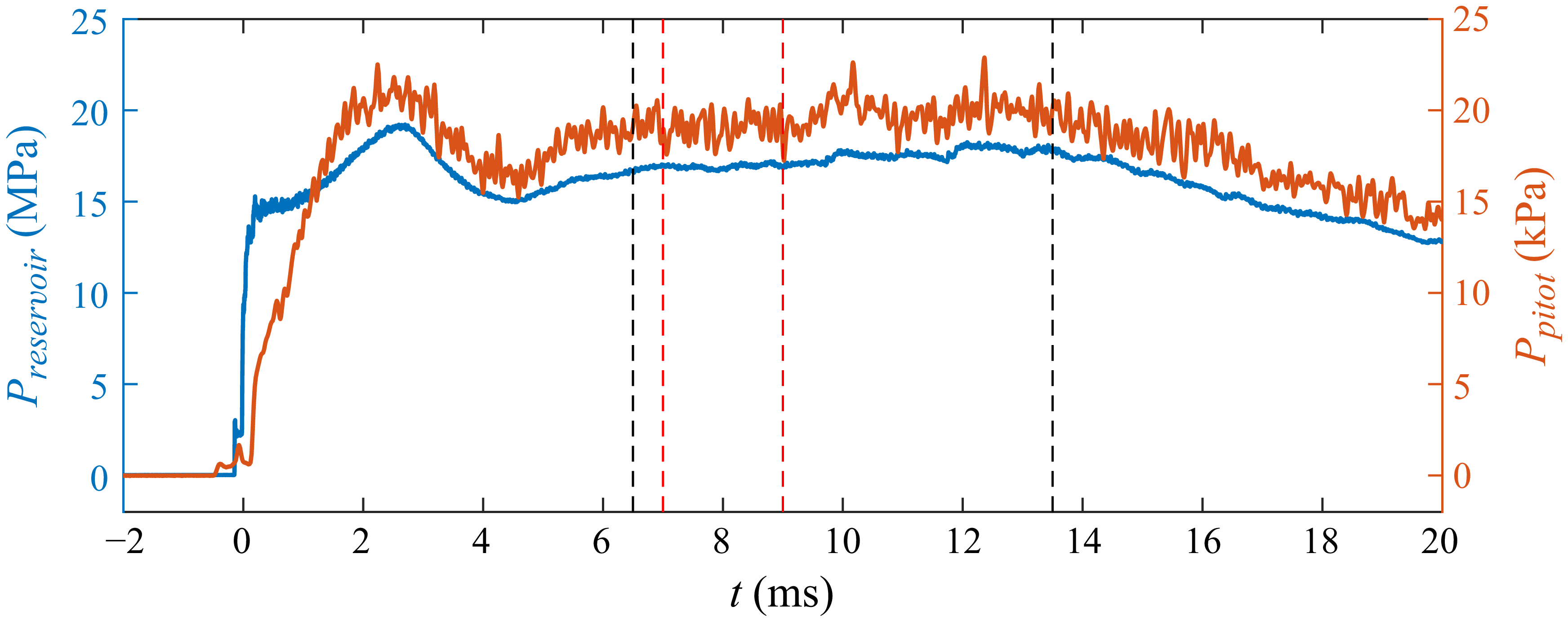
across different tests. Figure 1 shows typical traces of reservoir pressure and Pitot pressure under the current flow condition. The maximum effective test duration is approximately 7 ms, during which the relative standard deviations of the reservoir pressure and Pitot pressure are about 2.4
 $\%$
and 4.2
 $\%$
, respectively. For a narrower time range, such as
 $t$
= 7–9 ms (as used in the subsequent mean heat transfer analysis), the standard deviation values are even smaller at 0.7
 $\%$
and 3.7
 $\%$
, respectively.
Incoming flow parameters.

Typical traces of reservoir pressure (blue line) and Pitot pressure (orange line) under the present flow conditions. Here
 $t$
= 0 ms corresponds to the breaking of the secondary diaphragm. To facilitate comparison, the Pitot pressure trace is time shifted to account for the flow passage through the nozzle, aligning it with the reservoir pressure trace. The maximum effective test duration is indicated by the black dashed lines. The time range used for subsequent time-averaged results is indicated by the red dashed lines.

Schematic of fast TSP measurement on the compression ramps.

The test model consisted of a frame, a flat plate module and replaceable compression ramp modules, as shown in figure 2. The aluminium frame measured 600 mm in length, 300 mm in width, featuring a
 $24^\circ$
steel leading edge with a radius of 0.2 mm mounted at the front. The flat plate and compression ramp modules were fabricated from fibre-reinforced plastic, with a width of
 $w$
= 180 mm. The compression ramp modules featured a ramp angle of
 $\alpha$
=
 $34^\circ$
, sweep angles of
 $\chi$
=
 $0^\circ$
,
 $15^\circ$
,
 $30^\circ$
and
 $45^\circ$
, and a height of 80 mm. The trailing edge of the flat plate module was positioned
 $L=350$
mm downstream from the frame’s leading edge. For the unswept ramp module, its leading edge was aligned flush with the trailing edge of the flat plate module. For the swept ramp modules, there is a triangular panel between the flat plate and the swept ramp, with its leading edge aligned flush with the trailing edge of the flat plate module. The origin of the Cartesian coordinate system used in the present work is defined as the centre point at the trailing edge of the flat plate module, or equivalently, the centre point of the leading edge at the ramp module, as shown in figure 2.
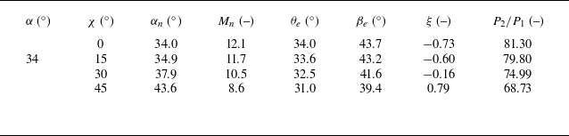
The inviscid analysis parameters for the examined swept ramps are listed in table 2. Here,
 $M_n$
and
 $\alpha _n$
denote the Mach number and ramp angle normal to the hinge line, respectively, with
 $M_n=M_{\infty }\cos \chi$
,
 $\alpha _n=\arctan (\tan \alpha /\cos \chi )$
;
 $\theta _e$
and
 $\beta _e$
denote the deflection angle and shock angle, respectively, in the effective plane with an incoming Mach number of
 $M_{\infty }$
, according to Domel’s theory (Domel Reference Domel2016);
 $\xi$
represents the detachment similarity parameter, commonly used in swept interactions to describe the inviscid shock shape (Settles & Kimmel Reference Settles and Kimmel1986). Details regarding the explanations and determination of
 $\theta _e$
,
 $\beta _e$
and
 $\xi$
are provided in Appendix A. As shown in table 2, increasing the sweep angle leads to a smaller effective shock angle
 $\beta _e$
and a lower pressure ratio across the inviscid shock, but results in a higher detachment similarity parameter, indicating a greater tendency for shock detachment. The critical value
 $\xi _c$
equals 0.85, beyond which the inviscid shock is detached. Since all values of
 $\xi$
in table 2 are below
 $\xi _c$
, the inviscid shock remains attached for all ramps investigated in this study.
Inviscid parameters.

2.2. Fast TSP measurement system
The fast TSP employed in this study was developed in-house, using dichlorotris(1,10-phenanthroline) ruthenium(II) (Ruphen) as the luminophore and automobile clearcoat as the binder (Liu et al. Reference Liu, Zhuang, Zhang, Wang, Liu and Peng2024). The luminophore has a lifetime of about 2
 $\unicode {x03BC}$
s at ambient temperature, and its excitation band spans from 400 to 450 nm, with an emission peak at approximately 600 nm. This TSP exhibits a high temperature sensitivity of
 $-2.3\,\%$
K−1 at ambient temperature, defined as the change in intensity ratio
 $I/I_{\textit{ref}}$
per unit increase in temperature, as shown by the temperature calibration curve on the top right of figure 3. The inherent dynamic heat flux response time for TSP is within 43
 $\unicode {x03BC}$
s. This estimation is the sum of the time delay (23
 $\unicode {x03BC}$
s) between the heat flux gauge and TSP results without temporal filtering, and the dynamic response time (20
 $\unicode {x03BC}$
s) of the heat flux gauge. It should be noted that the dynamic heat flux response is distinct from the dynamic temperature response, and minimally affected by the paint thickness (Schramm & Hilfer Reference Schramm and Hilfer2018; Liu et al. Reference Liu, Zhuang, Zhang, Wang, Liu and Peng2024). But it will be affected by the temporal filtering, which is usually applied to reduce the measurement noise. In the present work, the comparison of heat flux histories shown in the bottom right of figure 3 indicates a delay of around 100
 $\unicode {x03BC}$
s between the temporal filtered TSP result and the heat flux gauge result. Therefore, the TSP demonstrates a sufficiently fast response to capture the quasi-steady heat flux fields discussed in § 3.2. In the preparation of the test model, a white screen layer was pre-applied with a thickness of a few hundred microns, and then the fast TSP was sprayed to the model surface to form a uniform layer approximately 40
 $\unicode {x03BC}$
m thick.
As illustrated in figure 2, the fast TSP measurement system comprised three high-power light-emitting diodes with a central wavelength of 405 nm as the excitation source and a Photron SA-Z high-speed camera. The camera was equipped with a Nikon f/1.2 50 mm lens and 570 nm long pass filter. The regions of interest (ROIs) were located on the ramp, where significant aerothermal effects were observed. The sampling rates were set as 75, 70, 60 and 50 kHz, decreasing with sweep angle as the ROI expanded. The spatial resolution of the TSP images was around 0.4 mm pixel−1. In addition to the TSP measurements, several platinum thin-film heat flux gauges with a response time less than 20
 $\unicode {x03BC}$
s were installed along the centreline of the plate and ramp to simultaneously record local heat flux histories. These measurements also served as a basis for the in-situ calibration of the TSP.
General data processing procedure of a fast TSP measurement.

As shown in figure 3, the data processing procedure for fast TSP measurements involves two primary steps: (i) converting intensity images to temperature fields, (ii) determining heat flux fields by solving the inverse heat conduction problem. In the first step, following the image registration between the wind-off and wind-on images, the intensity ratio sequence is calculated and subsequently converted into temperature fields based on the prior temperature calibration. A spatial mean filter with a size of 5
 $\times$
5 pixels and a seven-point temporal mean filter are then applied to enhance the signal-to-noise ratio (SNR) of the temperature fields. In the second step, a transient in-situ calibration method, proposed in our previous work (Liu et al. Reference Liu, Zhuang, Zhang, Wang, Liu and Peng2024), is employed to inverse the time-resolved heat flux fields. The essence of this method is to determine the thermal properties and thickness of the TSP based on in-situ heat flux gauges by solving the following optimisation problem:
 \begin{equation} \min _{{\boldsymbol{\beta }}}G\left ( \boldsymbol{\beta }\right ) = \left \|\boldsymbol{\theta }_{\textit{TSP}}-{\boldsymbol H}\left (\boldsymbol{\beta }\right )\boldsymbol{q}_g \right \|_{2}^{2}. \end{equation}
Here,
 $\boldsymbol{\theta }_{\textit{TSP}}$
represents the temperature rise histories of TSP near the gauges,
 $\boldsymbol {H}$
is the temperature response matrix for the double-layer semi-infinite heat conduction model, which depends on the TSP’s parameters
 $\boldsymbol{\beta }$
, and
 $\boldsymbol{q}_g$
denotes the heat flux histories measured by the gauges. The Levenberg–Marquardt algorithm is employed to solve this optimisation problem. Once
 $\boldsymbol{\beta }$
is obtained, the heat flux history at each pixel can be inverted using
 $\boldsymbol {H}^{-1}\boldsymbol{\theta }_{\textit{TSP}}$
. A more detailed description and specific implementation of this method can be found in our previous work (Liu et al. Reference Liu, Zhuang, Zhang, Wang, Liu and Peng2024). Finally, a temporal filter length of 11–15 points (depending on the sampling rate) was applied to further improve the SNR of the heat flux results. The uncertainty of heat flux from the TSP measurement is approximately
 $\pm 7.5\,\%$
. The heat transfer coefficient
 $C_H$
is used to normalise the heat flux results, which is defined as
 \begin{equation} C_H = \frac {q}{\rho _\infty U_\infty c_p\left (T_0-T_w \right )} ,\end{equation}
where
 $q$
is the surface heat flux,
 $T_w$
= 292 K represents the wall temperature and
 $c_p$
= 1040 J kg–1 K is the specific heat capacity at constant pressure for nitrogen. The values of
 $\rho _\infty$
,
 $U_\infty$
and
 $T_0$
are provided in table 1.
3. Results and discussion
3.1. Boundary-layer state
First, to assess the state of the incoming boundary layer, the streamwise distributions of the time-averaged heat transfer coefficient along the flat plate’s centreline for different configurations are analysed, as shown in figure 4(a). These data were obtained in separate experiments using a metal flat plate module equipped with a coaxial thermistor array. Here, the distributions for
 $\chi$
=
 $45^\circ$
and
 $30^\circ$
are used to examine the boundary-layer state prior to the interaction, which closely follow the laminar theory in trend, albeit with slightly higher amplitudes. The fact that the incoming boundary layer remains laminar upstream of
 $x/L = 0$
with a swept compression ramp suggests a similar boundary-layer state in the absence of a downstream ramp. Therefore, for
 $\chi$
=
 $15^\circ$
and
 $0^\circ$
, despite the earlier start of interaction, the incoming boundary layer upstream of the interaction zone should also be laminar. In addition, for
 $\chi$
=
 $0^\circ$
, the streamwise distribution of heat transfer shows a significant decrease between
 $x/L= -0.6$
and
 $-0.5$
, followed by a gradual and then rapid increase. Downstream of
 $x/L = -0.2$
, the amplitude exceeds the laminar counterpart, which seems distinct from the purely laminar interaction (Gai & Khraibut Reference Gai and Khraibut2019).
(a) Streamwise distributions of the time-averaged heat transfer coefficient along the flat plate’s centreline. (b) Heat flux histories beneath the upstream boundary layer (
 $x/L= -0.54$
) and the reattached boundary layers (
 $x/L=$
0.26, 0.33, 0.38, 0.52 for
 $\chi$
=
 $0^\circ$
,
 $15^\circ$
,
 $30^\circ$
and
 $45^\circ$
, respectively) at the ramp’s centreline.

Subsequently, the state of the reattached boundary layer at the ramp’s centreline is examined. This is necessary for the swept configurations, because the above thermistor data within the finite streamwise range on the flat plate cannot indicate whether a transition has occurred. The heat flux histories beneath the reattached boundary layer measured by the thin-film heat flux gauges are shown in figure 4(b). For comparison, the heat flux history beneath the upstream laminar boundary layer for
 $\chi$
=
 $45^\circ$
is also included. The results reveal that the heat flux fluctuations in the upstream boundary layer are minimal, closely matching the measurement noise level. In contrast, significant heat flux fluctuations are evident downstream of reattachment. This notable difference implies that the reattached boundary layers are no longer in a laminar state, namely, the transition occurs near or upstream of the measuring points at the centreline.
In summary, the examined SBLIs feature a laminar incoming boundary layer, while the reattached boundary layer in the specified region is transitional. Following Threadgill, Little & Wernz (Reference Threadgill, Little and Wernz2021), these interactions can be classified as the ‘transitional SBLI,’ representing an intermediate state between purely laminar and purely turbulent interactions. However, compared to 2-D transitional SBLIs, the transition process in 3-D interactions is more complex, exhibiting spanwise variation in transition onset, as discussed in § 3.2. Consequently, although not all regions of the boundary layer over the ramp become transitional or display the same intermittency at a given downstream location, most of the spanwise range shows signs of transition and distinct heat flux patterns compared to purely laminar interactions, justifying the classification of the examined SBLI as a transitional interaction.
3.2. Time-averaged heat transfer characteristics
Figure 5 presents the time-averaged heat transfer distributions during the quasi-steady state (
 $t$
= 7–9 ms) for various sweep angles. These distributions reveal complex aerothermal effects and distinct 3-D features on the ramps. To gain an initial understanding of the flow structure and its link to the global heat transfer distribution on the ramp, the results for the unswept configuration are first examined alongside an instantaneous schlieren image (taken at a 3.3
 $\unicode {x03BC}$
s exposure time). As shown in figure 6(a), the incoming laminar boundary layer is unable to withstand the adverse pressure gradient imposed by the ramp-induced shock, resulting in a considerably large separation bubble. The bubble on the ramp impedes the convective heat transfer to the wall, leading to a low heat transfer coefficient in the separated region as indicated in figure 5(a). Above the separated region, the shear layer, separation shock (SS) and leading edge shock (LS) can be observed. As the separated shear layer reattaches to the ramp, a strong reattachment shock (RS) is observed near the reattachment point (at
 $x/L = 0.11$
or at
 $x/w = 0.21$
in figure 5
a). A heat flux peak is identified downstream of reattachment, attributed to the thinning of the reattached boundary layer (Simeonides & Haase Reference Simeonides and Haase1995). Further downstream, the RS interacts with SS and LS consecutively. Although the details of these shock–shock interactions cannot be directly observed from the schlieren image due to the limited size of the optical window, they can be inferred from the global heat transfer distribution. As shown in figure 5(a), the heat transfer coefficient experiences two distinct, rapid drops under the influence of impinging waves generated by the SS-RS and LS-RS interactions, respectively. This indicates that the impinging waves are expansion waves, and the aforementioned shock–shock interactions can be classified as type VI, as defined by Edney (Reference Edney1968). The region between the first heat flux peak and the first rapid drop due to the SS-RS interaction is subsequently referred to as the high heat transfer region for convenience, as illustrated in figure 5(a). Heat flux streaks are clearly observed in this region, which have been reported in previous investigations of hypersonic compression ramp flows (Ishiguro et al. Reference Ishiguro, Nagai, Asai and Nakakita2007; Gonzales et al. Reference Gonzales, Suzuki and Sakaue2020). These streaks are likely caused by Görtler vortices (Benay et al. Reference Benay, Chanetz, Mangin, Vandomme and Perraud2006; Cao et al. Reference Cao, Klioutchnikov and Olivier2019) considering their variations with the sweep angle as discussed later. However, to avoid controversy, these structures are referred to as Görtler-like vortices throughout this paper.
Time-averaged heat transfer coefficient distributions on the ramps; (a–d)
 $\chi$
=
 $0{-}45^\circ$
.

(a) Schlieren image of the unswept ramp. (b) Illustration of flow structures in a transitional SBLI on a swept compression ramp.

For the swept configurations, schlieren images are unavailable due to the obstruction of the optical path. Since the global heat transfer distributions of the swept and unswept configurations exhibit certain similarities, the 2-D flow structure previously described can still serve as a valuable reference for studying the swept configurations. As shown in figure 5(b–d), the separated region (low heat transfer region) at the ramp bottom displays a nearly linear expansion along the span. Its streamwise spacing narrows as the sweep angle increases. Similar trends are observed for the high heat transfer regions downstream of reattachment. Heat flux streaks are also visible across the high heat transfer region, and their intensity varies with the sweep angle. Additionally, a region of low heat transfer is observed near the ramp’s leading side. The streamwise heat transfer distributions in the adjacent region show clear differences downstream of reattachment. The following discussion will elaborate on the aerothermal effects for the swept configurations from these aspects: (i) heat flux peaks related to reattachment and shock structure, (ii) heat flux streaks following reattachment, (iii) spanwise heat flux variations induced by differences in boundary-layer state. The flow structures for the swept configurations inferred from the global heat transfer distributions and the previous 2-D flow structure are depicted in figure 6(b) to support the subsequent analysis.
(a) Streamwise distributions of the heat transfer coefficient at
 $z/w = 0.02$
for various sweep angles. (b) Amplitude variation of the first heat flux peak with sweep angle (normalised by the value for
 $\chi$
=
 $0^\circ$
). Here
 $x_c$
denotes the streamwise coordinates of the corner. The subscript
 $p$
and 0 represent the peak and
 $\chi$
=
 $0^\circ$
. The fading bars in (a) and error bars in (b) represent the measurement uncertainty of
 $7.5\,\%$
. The laminar and turbulent predictions are calculated based on the 1.13 and 0.85 powers of the pressure ratio
 $P_2/P_1$
across the inviscid shock, respectively.

Firstly, to analyse the influence of sweep angle on the heat flux peak, the streamwise distributions of the heat transfer coefficient near the centreline (at
 $z/w = 0.02$
) are extracted and presented in figure 7(a). As the sweep angle increases, the first heat flux peak shifts upstream with a reduced amplitude. Given that the first heat flux peak roughly indicates reattachment, the upstream movement with increasing sweep angle suggests a similar trend for the reattachment location. This is in contrary to the observations in turbulent swept interactions with cylindrical symmetry (Ceci et al. Reference Ceci, Palumbo, Larsson and Pirozzoli2024) and quasi-conical symmetry (Erengil & Dolling Reference Erengil and Dolling1993). In these turbulent interactions, the increased sweep angle results in a larger separation scale with the reattachment location moving downstream. The opposing trend observed in this study can be attributed to the intensified transitional effects in the separated shear layer, which are partially contributed by the increasing local Reynolds number at the corner (
 ${Re}_{x_c}$
). Furthermore, the amplitude variation of the first heat flux peak with sweep angle is examined and illustrated in figure 7(b). It should be noted that the error bars associated with the amplitude represent the measurement uncertainty and do not account for the unsteadiness caused by heat flux streaks. As the sweep angle increases, the amplitude of the first peak decreases, similar to the variation of pressure ratio across the inviscid shock. Previous studies have established a power-law relationship between the maximum heat flux ratio and the pressure ratio downstream of reattachment, with exponents of 1.13 for laminar interactions (Hung & Barnett Reference Hung and Barnett1973) and 0.85 for turbulent interactions (Back & Cuffel Reference Back and Cuffel1970; Zuo Reference Zuo2023; Tang et al. Reference Tang, Xu, Li and Ren2024). As shown in figure 7(b), the results in the present work generally follow the trend in the simplified analysis using the inviscid pressure ratios shown in table 2. It should be noted that the above analysis simplifies the separation and reattachment shocks as a single inviscid shock, and does not account for the heat flux peak overshoot (Sandham et al. Reference Sandham, Schülein, Wagner, Willems and Steelant2014) in the viscous interactions and the effects of heat flux streaks, which leads to the discrepancies between the experimental results and theoretical predictions.
In addition to the first peak just downstream of reattachment, a stronger second peak is observed on the
 $45^\circ$
swept ramp. Following this second peak, the heat transfer coefficient decreases rapidly. Since the second peak is located near the SS-RS interaction zone, it is likely the result of a type V shock–shock interaction. In this scenario, the generated transmitted shock is subsequently reflected by the ramp and the slip line to produce an expansion wave (Edney Reference Edney1968), and the sequential impingement of shock and expansion waves forms a peak in heat transfer. Previous investigations on the double-wedge flow show that the shock–shock interaction will change from type VI to type V when the shock strength is enhanced (Ishiguro et al. Reference Ishiguro, Nagai, Asai and Nakakita2007; Li, Zhu & Luo Reference Li, Zhu and Luo2014). For the swept ramps, as the sweep angle increases, although the pressure ratio across the inviscid shock decreases, the inviscid shock tends to detach, as analysed in Appendix A. This tendency of shock detachment is somewhat similar to the effect of increasing AOA for the double-wedge flow. Further evidence for this argument is the global heat transfer distribution on a
 $38^\circ$
compression ramp, which shows a similar double peak pattern for a lower sweep angle (
 $\chi$
=
 $30^\circ$
) under the same incoming flow condition (see figure 14). It can be anticipated that more complex shock–shock interactions will emerge as the ramp angle or the sweep angle further increases, similar to the influence of the AOA on the shock–shock interaction in hypersonic compression ramp flows as reported by Ishiguro et al. (Reference Ishiguro, Nagai, Asai and Nakakita2007). Additionally, preliminary inviscid simulations of the wedge-swept wedge, as presented in Appendix B, confirm that increasing the sweep angle can cause a transition in the shock–shock interaction type. Further research is required to fully understand the sweep effects on the shock–shock interaction in swept compression ramp flows.
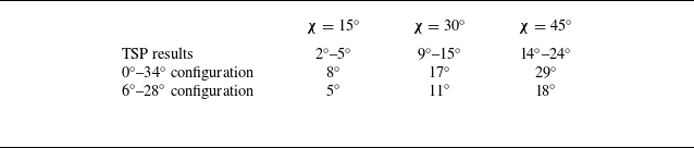
Secondly, the heat flux streaks following reattachment are discussed. These streaks can be seen across a broad area downstream of reattachment, with their traces particularly pronounced within the high heat transfer region. The orientations of these streaks are extracted from the global heat transfer maps, which can be regarded as the streamline directions. It is observed that the streak angles generally increase with
 $z/w$
. Specifically, these angles are quantified by calculating the dot product between the unit vectors representing the streaks and the ramp’s centreline. These vectors are obtained by selecting feature points along the streaks and the centreline (where the heat flux gauges are located). The specific values of streak angles for varying sweep angles are listed in table 3, along with the streamline deflection angles calculated based on Domel’s theory (Domel Reference Domel2016), as introduced in Appendix A. In addition to the single
 $34^\circ$
ramp, we also consider the case where the incoming flow is first deflected by a
 $6^\circ$
wedge (estimated from the separated region visible in the schlieren image of the unswept ramp) before encountering the swept wedge. In this scenario, we neglect the effect of shock–shock interaction on the streamline deflection. As shown in table 3, the streak angles extracted from the TSP results are smaller than the inviscid streamline deflection angles for the single
 $34^\circ$
ramp. This discrepancy is largely attributed to the omission of the flow deflection caused by the separated region. By modelling the separated region as an initial
 $6^\circ$
wedge, the inviscid deflection angles of the streamline on the second swept wedge show good agreement with the experimental observations.
Comparison between the streak angles from TSP results and the inviscid streamline deflection angles (shown in the third and fourth rows). The
 $0^\circ{-}34^\circ$
configuration refers to a single
 $34^\circ$
compression ramp, while the
 $6^\circ{-}28^\circ$
configuration represents a wedge-swept wedge with streamwise deflection angles of
 $6^\circ$
in the first unswept wedge and
 $28^\circ$
in the second swept wedge, respectively.

(a) Time-averaged heat transfer coefficient distributions along the upstream peak line for various sweep angles, and (b) corresponding spatial Fourier transformation results.

To further assess the variation in the intensity and wavelength of heat flux streaks, the heat transfer distribution along the upstream peak line is extracted and presented in figure 8(a). The upstream peak line is determined by linearly fitting the positions of the first heat flux peaks at various spanwise locations. The results show that as the sweep angle increases, the spanwise variation of heat streaks tends to decrease, which can also be attributed to the intensified transitional effects mentioned earlier in connection with the upstream motion of the reattachment location. Moreover, the wavelengths of these streaks, indicated by the distance projected on the
 $z$
axis between two adjacent peaks, range from 0.057
 $w$
to 0.065
 $w$
and show little dependency on the spanwise location and sweep angle. A spatial Fourier transformation is then performed on the distributions shown in figure 8(a) to obtain quantitative results. As shown in figure 8(b), for the unswept ramp, a distinct peak appears at a wavenumber of approximately
 $k_z$
= 96 m
 $^{-1}$
. This wavenumber corresponds to a wavelength of 0.058
 $w$
, which is generally consistent with the spacing between adjacent peaks labelled in figure 8(a). As the sweep angle increases, this local peak at about
 $k_z$
= 96 m
 $^{-1}$
persists, but its amplitude decreases and nearly vanishes for the
 $45^\circ$
swept ramp. These results confirm the weak dependence of the streak’s dominant wavelength on the sweep angle. The above evidence suggests the convective mechanism (rather than the global instability) is mainly responsible for these streaks, because the wavelength of streaks driven by global instability would depend on the separation scale (Hao et al. Reference Hao, Cao, Wen and Olivier2021). Specifically, the convective mechanism is most likely the Görtler instability, which is highly sensitive to the imperfections of the leading edge that are virtually inevitable in experiments (Ginoux Reference Ginoux1971; de la Chevalerie et al. Reference de la Chevalerie, Fonteneau, De Luca and Cardone1997). The disturbances induced by these imperfections are amplified by Görtler instability downstream of reattachment, leading to a nearly constant wavelength of the streaks regardless of the interaction strength. In the present study, although no obvious defect can be found on the main span of the leading edge, the extreme receptivity of Görtler instability to the imperfections of the leading edge still very likely induces the streamwise vortices and heat flux streaks (Roghelia et al. Reference Roghelia, Olivier, Egorov and Chuvakhov2017; Lugrin et al. Reference Lugrin, Nicolas, Severac, Tobeli, Beneddine, Garnier, Esquieu and Bur2022). The above observations of heat flux streaks are also reminiscent of the findings reported by Lugrin et al. (Reference Lugrin, Nicolas, Severac, Tobeli, Beneddine, Garnier, Esquieu and Bur2022). They studied the influence of the Reynolds number on the heat flux streaks in the transitional SBLI on a hollow cylinder flare using infrared thermometry. Their results showed that as the Reynolds number increased, the heat flux peak moved upstream, and the heat flux streaks were weakened with the dominant wavelength almost unchanged. In addition, figure 8(b) shows a broadband feature with wavenumbers between
 $k_z$
= 35–70 m
 $^{-1}$
, highlighted by the cyan rectangle, which is present in each case. Moreover, it is worth noting that the spanwise heat flux variations caused by heat flux streaks observed in the time-averaged results depend on the averaging time range, due to the unsteadiness of heat flux streaks, as explained in Appendix C.
Heat transfer coefficient distributions along lines originating from the point at
 $y/w=0.39$
and
 $z/w=-0.5$
, and oriented parallel to the upstream peak line for various sweep angles. These lines are located downstream of the LS-RS interaction region, as illustrated in the top left subplot for the
 $45^\circ$
swept ramp, shown as an example.

Finally, the focus is turned to the rich features of spanwise heat transfer variations further downstream of the reattachment region. The spanwise heat transfer distributions originating from the point at
 $y/w=0.39$
and
 $z/w=-0.5$
for the half-ramp (
 $z/w$
from
 $-0.50$
to 0) are presented in figure 9. The results for the unswept and swept configurations show substantial differences. For the unswept ramp, the heat transfer coefficient remains constant near the ramp centre and monotonically decreases as
 $z/w$
varies from
 $-0.33$
to approximately
 $-0.5$
, indicating the flow spillage effect due to the ramp’s finite width (Threadgill, Little & Wernz Reference Threadgill, Little and Wernz2019; Sadagopan et al. Reference Sadagopan, Huang, Jirasek, Seidel, Pandey and Casper2023). In contrast, for the swept ramps, the distributions exhibit a ‘V’-shaped trend in the
 $z/w$
range of
 $-0.5$
to
 $-0.33$
, with a lower minimum heat transfer coefficient than that for the unswept ramp. Moreover, as the sweep angle increases, the minimum heat transfer coefficient further decreases, and the low heat transfer region expands in the spanwise direction. The flow spillage effect does not account for this trend, as it would diminish with increasing sweep angle due to lower pressure on the swept ramp. Other inviscid effects include the expansion effect from streamline deflection in this region and the compression effect from the free stream directly attaching to the ramp. According to the inviscid simulation results in Appendix B, these competing effects lead to a lower temperature near the leading side of the
 $15^\circ$
and
 $30^\circ$
swept ramps (see figures 16
b and 16
c), where the expansion effect dominates. However, for the
 $45^\circ$
swept ramp, the compression effect prevails and results in a high temperature region near the leading side (see figure 16
d), which is contrary to experimental observations. Therefore, these inviscid effects are not the primary reasons for the low heat transfer region near the ramp’s leading side. Instead, the dominant factor is likely the variation in boundary-layer intermittency. Near the leading side, the boundary layer attached to the ramp is either laminar or, at least, has low intermittency. Away from the leading side, the intermittency rises in the boundary layer, resulting in higher heat transfer (the right-hand side of the V shape in figure 9). To clarify this point, the streamwise heat flux distribution at
 $z/w = -0.45$
for
 $\chi$
=
 $30^\circ$
, across the low heat transfer region, is presented in figure 10(a) (labelled by the reference line). As
 $(x-x_p)/w$
increases from 0.15 to 0.4, the heat transfer coefficient gradually decreases and is significantly lower than that in the adjacent region, indicating the development of a laminar boundary layer. An interesting detail further confirms the laminar state of the boundary layer in the specific area of the low heat transfer region. During the wind tunnel tests, a diaphragm fragment accidentally struck this region on the
 $30^\circ$
swept ramp and caused a minor defect. Consequently, a trail of increased heat flux was observed downstream of this defect (see figure 20), matching the transition phenomenon caused by an isolated roughness element in the laminar boundary layer (Tirtey, Chazot & Walpot Reference Tirtey, Chazot and Walpot2011; Liu et al. Reference Liu, Wang, Dong, Xia, Chen and Zhao2021). Similar laminarization regions have also been found in fully turbulent swept SBLIs (Adler & Gaitonde Reference Adler and Gaitonde2019; Zhang et al. Reference Zhang, Guo, Dang and Li2022), though they are less pronounced than those observed in the present study. Additionally, the region of high heat transfer very close to the edge of
 $z/w = -0.5$
(the left-hand side of the V shape in figure 9) can be attributed to the stagnation effect, which is also absent in the unswept ramp.
(a) Heat transfer coefficient distributions along various lines illustrated in the upper right subplot for
 $\chi$
=
 $30^\circ$
. The reference line originates from
 $z/w = -0.45$
on the hinge line and is parallel to the edge of the swept ramp. The square symbols represent the minimum values of the quadratic polynomial fitting curves indicated by the black dashed line. (b) Heat transfer coefficient distributions along the line parallel to the upstream peak line with a streamwise distance of 0.3
 $w$
for
 $\chi$
=
 $30^\circ$
.

Another key observation that highlights the transitional nature of the SBLI examined in this study is the spanwise heat flux variation on the swept ramp between its centreline and the aforementioned laminar region. The results for
 $\chi$
=
 $30^\circ$
are taken as an example, and the heat transfer distributions along various streamlines are extracted and presented in figure 10(a). These streamlines originate from different spanwise locations on the hinge line and are oriented based on the nearby heat flux streaks. As previously discussed, the heat transfer distribution along the first line near the edge (
 $z/w = -0.45$
, the reference line in blue) indicates the development of a laminar boundary layer on the ramp. In contrast, the heat transfer distribution along the adjacent oblique streamline with the same origin (indicated by the orange line) first drops and then gradually rises, as
 $(x-x_p)/w$
increases from 0.15 to 0.4. This trend indicates the occurrence of a boundary-layer transition near the location of the minimum heat transfer coefficient. As these streamlines move further away from the edge of the leading side, the heat transfer distributions exhibit a similar trend in the range of
 $(x-x_p)/w$
= 0.15–0.4, with an increase in the overall amplitude. Then, the minima of the quadratic polynomial curves fitted to the data in this region are extracted as an approximation of the transition onset location (noted by the squares in figure 10
a). It is observed that the minima move upstream towards the first peak as
 $z/w$
increases, indicating the spanwise variation trend of transition onset. It should be noted that as the streamline approaches the ramp centre, the aforementioned minimum falls into the SS-RS interaction region. This minimum can no longer reflect the transition onset, due to the coupled effects of shock–shock interaction and reattached boundary-layer transition on the heat transfer distribution. Alternatively, the heat transfer distribution along a line parallel to the upstream peak line (to ensure the same streamwise distance from the reattachment line) are extracted and presented in figure 10(b). Away from the laminar flow region, the heat transfer coefficient gradually increases with
 $z/w$
, before it becomes stable beyond
 $z/w$
= 0. This trend indicates that, away from the leading side, the transition onset of the reattached boundary layer initially shifts closer to the reattachment point, due to the larger streamwise separation scale and higher Reynolds number at the corner. At some point, the transitional effects within the separated shear layer become sufficiently strong, causing the boundary-layer transition immediately upon reattachment to the ramp. As a result, the transition onset is located very close to the reattachment point, leading to similar heat transfer characteristics in the downstream boundary layer. This ‘locking’ phenomenon of the transition onset at the reattachment point has also been observed in axisymmetric transitional SBLIs under increasing upstream disturbances (Lugrin et al. Reference Lugrin, Beneddine, Leclercq, Garnier and Bur2021).
3.3. Symmetry of heat transfer distribution
In this section the heat transfer symmetry on the swept ramps and the key factors disrupting the symmetry are discussed. The global heat transfer distributions presented in figure 5 show that the distance between the first heat flux peak and the hinge line increases linearly along the span for the swept ramps, suggesting a potential quasi-conical symmetry. To explore such symmetry, the global time-averaged heat transfer distributions are transformed from the Cartesian coordinate system into polar coordinates. The VCO is defined by the intersection of the hinge line and the upstream peak line. Based on this VCO, the displacement (
 $r$
) between a point on the ramp and the VCO, as well as the angle (
 $\phi$
) between the lines connecting this point to the VCO and the hinge line, are calculated. The transformed heat transfer distributions for the swept ramps are presented in figure 11(a,c,e). In contrast to typical turbulent scenarios (Zhang et al. Reference Zhang, Guo, Dang and Li2022), the VCO in the present transitional SBLIs is located farther from the swept origin, with a distance even exceeding the width of the swept ramp. This might be attributed to the larger separation scale for the transitional SBLIs. To further assess the symmetry, the circumferential distributions of heat transfer are extracted for various displacements
 $r/w$
. When taking these profiles, the inception region near the swept origin (where the heat flux peak location deviates from the linear upstream peak line) and the low heat transfer region near the ramp’s leading side are both avoided. As shown in figure 11(b,d,f), good consistency is observed in the heat transfer distributions upstream of the first peak across different
 $r$
, with the peak located at
 $\phi$
=
 $5.9^\circ$
,
 $5.4^\circ$
and
 $3.6^\circ$
for
 $\chi$
=
 $15^\circ$
,
 $30^\circ$
and
 $45^\circ$
, respectively. This consistency indicates a quasi-conical aerothermal symmetry upstream of reattachment for the transitional swept SBLIs examined.
Time-averaged results in polar coordinates, where the VCO is determined by the intersection of the upstream peak line and hinge line, for
 $\chi$
= (a,b)
 $15^\circ$
, (c,d)
 $30^\circ$
, (e,f)
 $45^\circ$
. Panels (a,c,e) show global heat transfer distributions and panels (b,d, f)show the circumferential distributions at different
 $r/w$
.

Compared with the consistent heat transfer behaviour upstream, varying degrees of divergence emerges downstream of the first heat flux peak. The most pronounced divergence occurs at
 $\phi \gt$
 $8^\circ$
for
 $\chi$
=
 $30^\circ$
, where the heat transfer coefficient increases significantly with
 $r/w$
. This trend reflects significant differences in the intermittency within the reattached boundary layer at the positions with the same
 $\phi$
but different
 $r/w$
, which can be associated with the movement of the transition onset discussed in § 3.2. Such divergence becomes more pronounced as the sweep angle increases from
 $\chi$
=
 $15^\circ$
to
 $30^\circ$
but significantly diminishes at
 $\chi$
=
 $45^\circ$
. This trend can be explained as follows. As the sweep angle increases, the spanwise variation in
 ${Re}_{x_c}$
and streamwise separation size is amplified, resulting in greater differences in the transition onset across the span. However, with further increases in sweep angle, stronger transitional effects shift the transition onset closer to the reattachment point and reduce its spanwise variation. Another notable divergence is related to the second peak in the high heat transfer region, particularly in the case of
 $\chi$
=
 $45^\circ$
, where the second peak amplitude surpasses that of the first peak as
 $r/w$
increases. This second peak is likely due to the type V shock–shock interaction as discussed before. As the sweep angle or the ramp angle further increases, the shock–shock interaction with varying type or intensity will produce different effects on the symmetry. In addition to the above divergences, fluctuations in the heat transfer coefficient are observed downstream of the first peak, disrupting the quasi-conical symmetry. These fluctuations originate from the heat flux streaks and their effects on the symmetry are especially pronounced for
 $\chi$
=
 $15^\circ$
, which is expected due to the strongest heat flux streaks in the swept configurations as explained in § 3.2. Moreover, considering that the strength of instantaneous heat flux streaks may exceed that of the time-averaged results (as explained in Appendix C), the disruption of the quasi-conical symmetry at some moments is likely to be even more pronounced.
4. Conclusion and remark
High-resolution heat transfer distributions, obtained through fast TSP measurements, reveal the complex aerothermal phenomena and sweep effects of a
 $34^\circ$
compression ramp at
 $M_{\infty }$
= 12.1, Re = 3.0
 $\times$
10
 $^{6}$
m
 $^{-1}$
. The streamwise heat flux distribution features a first peak located near the reattachment point, which shifts upstream with a diminishing amplitude as the sweep angle increases. A second heat flux peak emerges in the SS-RS interaction region on the
 $45^\circ$
swept ramp and is attributed to the transition of the shock–shock interaction from type VI to type V. These distinct sweep effects on the shock–shock interaction are similar to the effect of increased AOA for a 2-D ramp flow. Streamwise streaks lead to spanwise fluctuations in the heat flux downstream of reattachment, whose intensity drops with increasing sweep angle. These streaks are likely linked to Görtler vortices, since their projected wavelengths are not dependent on the spanwise position and sweep angle. The spanwise heat flux distributions downstream of the high heat transfer region are further complicated by the differences in the intermittency within the reattached boundary layer. The free stream directly attaches to the edge of the ramp’s leading side, producing a laminar region of low heat transfer. The area of this region expands, and its minimum heat flux decreases as the sweep angle increases. Adjacent to this laminar region, the transition in the boundary layer reattached from the separated shear layer is evident from the heat flux rise along the streamline. The transition onset shifts upstream toward and eventually locks at the reattachment point as the streamline moves away from the ramp’s leading side.
Regarding the symmetry of heat transfer on the swept ramps, a general quasi-conical symmetry is identified upstream of reattachment based on the VCO defined by the intersection of the upstream peak line and the hinge line. However, this symmetry is disrupted downstream due to spanwise variations in transition onset, shock–shock interaction and heat flux streaks. As the sweep angle increases, the impact of spanwise variations in transition onset initially increases and then diminishes, while the influence of the shock–shock interaction appears and the effect of heat flux streaks weakens. The finding also raises a question about the criteria of quasi-conical symmetry in transitional swept SBLIs. For turbulent swept interactions (Settles & Teng Reference Settles and Teng1984), the quasi-conical symmetry occurs when the inviscid shock is detached while the cylindrical symmetry occurs when the inviscid shock is attached. However, in the present work, the inviscid shocks for all swept ramps are detached, but the heat transfer distributions exhibit a partial quasi-conical symmetry. The larger separation scale in transitional SBLIs may render the previous symmetry criteria invalid.
It should be acknowledged that, although the fast TSP provided valuable global insights into the aerothermal effects in the transitional swept interactions, surface heat flux alone is far from enough to fully uncover the complex mechanisms driven by boundary-layer transition, shock–shock interaction and potential shear layer instability. Further efforts involving experiments using spatial flow field measurement techniques, high-fidelity simulations as well as stability analysis are required. Moreover, the swept ramps studied in the present work feature the same ramp angle but various sweep angles, while another interesting subject that deserves further investigation is the similarity between the swept ramps with various ramp angles and sweep angles but the constant inviscid shock strength, e.g. the same detachment similarity parameter or the same inviscid pressure ratio.
Supplementary movies
Supplementary movies are available at https://doi.org/10.1017/jfm.2025.10849.
Funding
This work was supported by the National Key Research and Development Program of China (No. 2019YFA0405300), the National Natural Science Foundation of China (NSFC No. 12227803) and the Gas Turbine Research Institute of Shanghai Jiao Tong University.
Declaration of interests
The authors report no conflict of interest.
Appendix A. Inviscid analysis
The following two methods are adopted for determining the parameters of the inviscid shock in the swept compression ramps. The first method applies the unswept shock relations in the plane normal to the hinge line by substituting the normal Mach number (
 $M_n$
) and normal ramp angle (
 $\alpha _n$
) into the 2-D oblique shock theory. The relationship between
 $\alpha _n$
,
 $M_n$
and the shock angle in the normal plane (
 $\beta _n$
) is
 \begin{equation} \tan \alpha _n=\frac {1}{\sin \beta _n}\left [\frac {\left (M_{n}^{2}\sin ^2\beta _{n}-1 \right )\sqrt {1-\sin ^2\beta _{n}}}{\frac {\gamma +1}{2}M_{n}^2-\left (M_{n}^{2}\sin ^2\beta _{n}-1 \right ) } \right ] \!,\end{equation}
where
 $\gamma$
is the ratio of specific heats for a perfect gas. The pressure ratio across the inviscid shock is then given by
 \begin{equation} \frac {P_2}{P_1}=1+\frac {2\gamma }{\gamma +1}\big (M_{n}^{2}\sin ^2\beta _{n}-1 \big ) .\end{equation}
The second method uses the generalised 3-D relation proposed by Domel (Reference Domel2016), which directly incorporates the sweep angle. The relationship between the ramp angle (
 $\alpha$
), incoming Mach number (
 $M_1$
), sweep angle (
 $\chi$
) and shock angle in the effective plane (
 $\beta _e$
) is
 \begin{equation} \tan \alpha =\frac {1}{\sin \beta _e}\left [\frac {\big (M_{1}^{2}\sin ^2\beta _{e}-1 \big )\sqrt {1-\sin ^2\beta _{e}\left (1+\tan ^2\chi \right )} }{\frac {\gamma +1}{2}M_{1}^2-\big (M_{1}^{2}\sin ^2\beta _{e}-1 \big )\left (1+\tan ^2\chi \right ) } \right ] \!.\end{equation}
The deflection angle in the effective plane (
 $\theta _e$
) is determined by
 \begin{equation} \tan \theta _e=\frac {\tan \alpha }{\tan \alpha \tan \beta _e\tan ^2\chi +\sqrt {1-\tan ^2\beta _e\tan ^2\chi } } .\end{equation}
The pressure ratio across the shock is given by
 \begin{equation} \frac {P_2}{P_1}=1+\frac {2\gamma }{\gamma +1}\big (M_{1}^{2}\sin ^2\beta _{e}-1 \big ) .\end{equation}
This is identical to the expression derived by the first method. However, Domel’s theory (Domel Reference Domel2016) provides additional insight into the actual streamline trajectories. The streamline deflection relative to the centreline can be determined using the dot product of the unit vectors representing the streamline (
 $\hat {a}_2$
) and the centreline (
 $\hat {a}_d$
), defined as
 \begin{align} \hat {a}_2 = \hat {i}\cos \theta _e-\hat {j}\sin \theta _e\tan \beta _e\tan \chi +\hat {k}\sin \theta _e\sqrt {1-\tan ^2\beta _e\tan ^2\chi },\\[-28pt] \nonumber \end{align}
 \begin{align} \hat {a}_d=\hat {i}\cos \alpha +\hat {k}\sin \alpha , \\[3pt] \nonumber\end{align}
where
 $\hat {i}$
,
 $\hat {j}$
and
 $\hat {k}$
are the unit vectors along the
 $x$
,
 $y$
and
 $z$
axes, respectively. The detailed derivations of these equations can be found in Domel (Reference Domel2016).
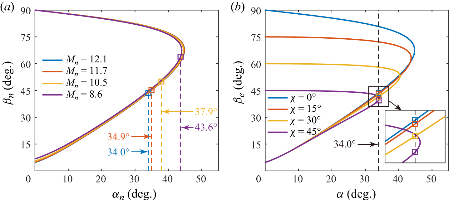
To illustrate the effect of sweep angle on inviscid shock properties, the shock relationships for the normal decomposition method and Domel’s method are presented in figures 12(a) and 12(b), respectively. In figure 12(a), increasing the sweep angle reduces the normal Mach number, yet the shock relationship curves remain nearly unchanged. However, the normal ramp angle rises rapidly, causing the weak solution (indicated by the square marker) to approach the maximum deflection angle, which suggests a greater tendency for the inviscid shock to detach at higher sweep angles. It is important to note that, due to the varying normal Mach number, the shock wave angle for the weak solution in figure 12(a) does not directly reflect the pressure ratio across the shock. According to (A2), the pressure ratio decreases with increasing sweep angle, as shown in table 2. In figure 12(b) the shock relationship changes significantly with increasing sweep angle, with the curves becoming compressed along both axes. At a fixed ramp angle of
 $34^\circ$
, the weak solution (square marker) exhibits a decreasing effective shock angle as the sweep angle increases, indicating a lower pressure ratio across the shock for a constant incoming Mach number. Additionally, the difference between the fixed ramp angle and the maximum deflection angle is reduced, further indicating a tendency for shock detachment. In summary, both methods give equivalent inviscid shock properties and yield consistent trends with increasing sweep angle.
Shock relationships for various sweep angles: (a) normal decomposition method; (b) Domel’s method (Domel Reference Domel2016).

To quantitatively characterise the extent of inviscid shock detachment, the detachment similarity parameter
 $\xi$
is used. This parameter has been extensively employed to correlate the inviscid shock shapes of different configurations in the study of turbulent swept SBLIs. As defined by Settles & Kimmel (Reference Settles and Kimmel1986),
 $\xi$
is given by
 \begin{equation} \xi =\frac {\alpha _n+C_1}{M_n (1-C_2 M_n)} ,\end{equation}
where
 $C_1$
and
 $C_2$
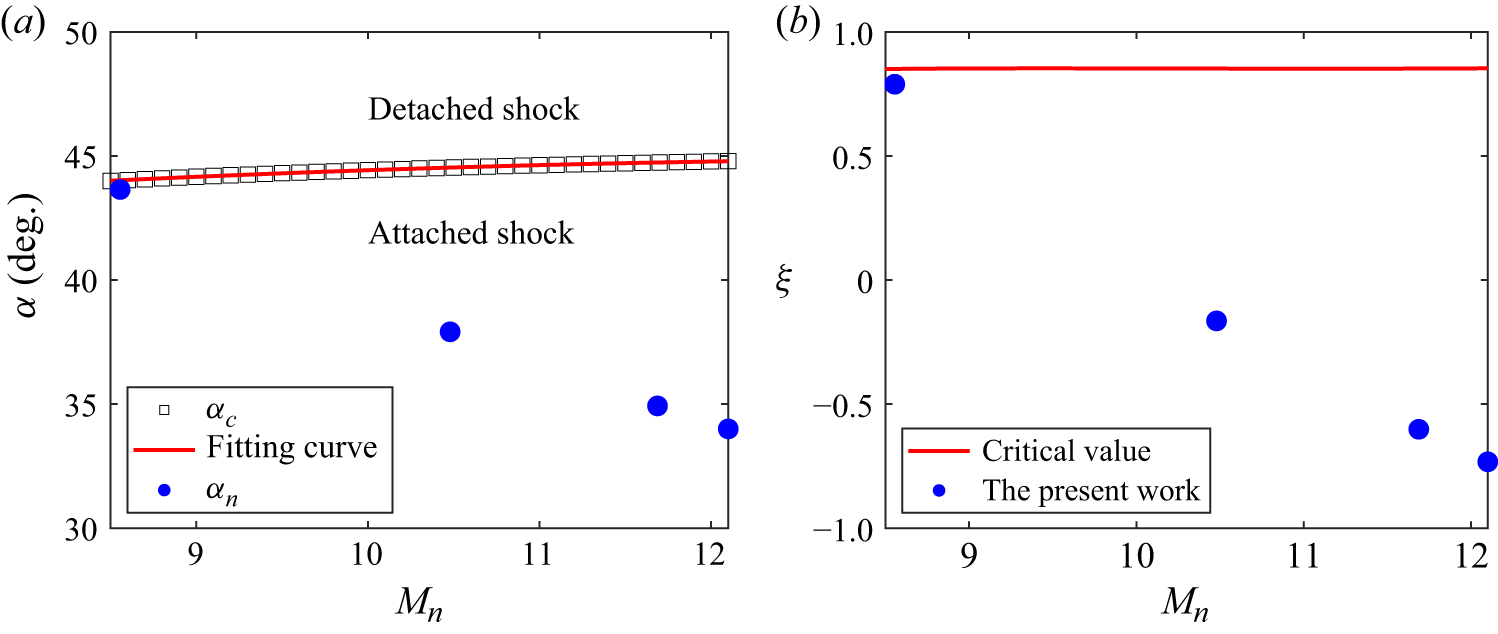
are obtained from a second-order polynomial curve fit of the expression for the maximum deflection angle by a wedge in the oblique shock theory. Figure 13(a) illustrates the critical detached deflection angle (
 $\alpha _c$
) across different normal Mach numbers. In this study, the normal ramp angles are found to be below the detached deflection angle. By fitting the relationship between the detached deflection angle and the normal Mach number (from
 $M_n$
= 8.5 to 12.2), the coefficients
 $C_1$
and
 $C_2$
are determined to be
 $-38.99$
and 0.036, respectively. Figure 13(b) illustrates the variation of the critical detachment similarity parameter
 $\xi _c$
with
 $M_n$
. It is observed that
 $\xi _c$
remains nearly constant at 0.85. For the sweep angles
 $\chi$
of
 $0^\circ$
,
 $15^\circ$
,
 $30^\circ$
and
 $45^\circ$
, the corresponding values of
 $\xi$
are calculated to be
 $-0.73$
,
 $-0.60$
,
 $-0.16$
and
 $0.79$
, respectively. All these values are below the critical threshold, indicating that the inviscid shock remains attached for all configurations.
(a) Relationship between the critical detached deflection angle
 $\alpha _c$
and the normal Mach number
 $M_n$
. The red line indicates the second-order polynomial fitting curve, while the blue solid circles represent the normal ramp angles for the configurations examined in this study. (b) Variation of the critical detachment similarity parameter
 $\xi _c$
with
 $M_n$
. The red line denotes the critical value and the blue solid circles correspond to the values for the configurations investigated in this work.

Appendix B. Transition in shock–shock interaction type
The global heat transfer distributions on a
 $38^\circ$
ramp with a
 $30^\circ$
sweep angle was measured under the same flow condition listed in table 1. As shown in figure 14, the high heat transfer region exhibits double heat flux peaks. This differs from the result for
 $\alpha$
=
 $34^\circ$
and
 $\chi$
=
 $30^\circ$
but resembles that for
 $\alpha$
=
 $34^\circ$
and
 $\chi$
=
 $45^\circ$
. It is inferred that the second peak arises from a type V shock–shock interaction, which replaces the common type VI interaction when the sweep angle or the ramp angle is sufficiently large. If the sweep and ramp angles are further increased, it is believed that other types of shock–shock interactions would occur.
Time-averaged heat transfer coefficient distributions on the ramp with
 $\alpha$
=
 $38^\circ$
and
 $\chi$
=
 $30^\circ$
.

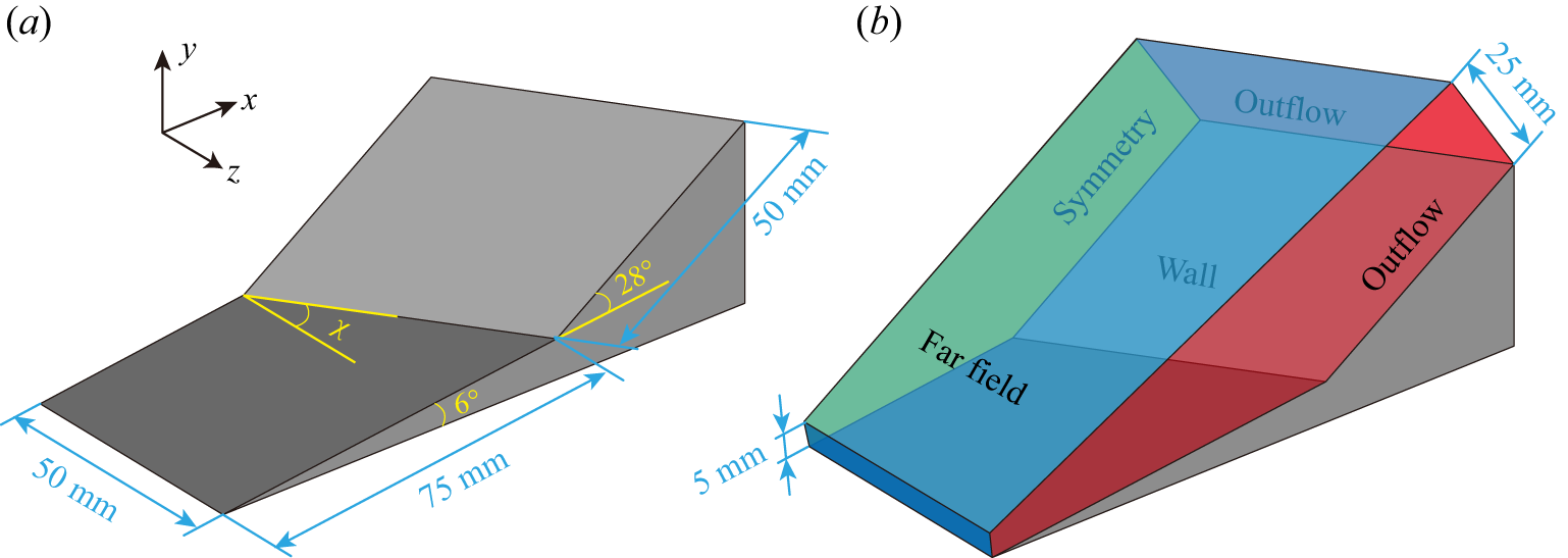
(a) Model geometry of the wedge–swept wedge configuration. (b) Computational domain and boundary conditions.

Surface temperature distributions normalised by the temperature on the first wedge and contours of the density gradient magnitude at the plane of
 $z$
= 40 mm; (a–d)
 $\chi$
= 0–45
 $^\circ$
. In the swept ramps, the streamlines near the leading side are superimposed.

To validate the occurrence of shock–shock interaction type transitions in swept SBLIs, a series of inviscid simulations are conducted on the wedge–swept wedge configuration shown in figure 15(a). In this setup, the first wedge serves as a surrogate for the boundary of the separated region in actual viscous flows. Its deflection angle is set to
 $6^\circ$
, estimated from the shear layer angle observed in the schlieren image for the unswept ramp. The second, swept wedge has a streamwise deflection angle (in the
 $x$
-
 $y$
plane) of
 $28^\circ$
, resulting in a total streamwise deflection angle of
 $34^\circ$
. The computational domain is illustrated in figure 15(b): the front and top planes are defined as far field boundaries, the left plane is set as a symmetry boundary (Zhang et al. Reference Zhang, Guo, Dang and Li2022) and the rear and right planes are specified as supersonic outflow boundaries (using simple extrapolation). The slip boundary condition is used at the wall. The computational grid consists of
 $921\times 301\times 360$
points (
 $N_x\times N_y \times N_z$
), with refinement near the wall and corner. Inviscid simulations are performed using the in-house multi-block parallel finite volume solver PHAROS (Hao, Wang & Lee Reference Hao, Wang and Lee2016; Hao & Wen Reference Hao and Wen2020). The modified Steger–Warming scheme (MacCormack Reference MacCormack2014) is used for inviscid flux calculations, and the implicit line relaxation method proposed by Wright, Candler & Bose (Reference Wright, Candler and Bose1998) is employed for pseudo-time marching. The incoming Mach number is set to 12.1.
Figure 16 presents the temperature distributions and density gradient magnitude contours for various sweep angles. A pronounced high temperature region is observed just downstream of the corner, resulting from the compression effect of the second wedge. As the sweep angle increases, the temperature in this region decreases, consistent with predictions from the inviscid theory. Downstream of the high temperature region, the temperature initially decreases and then slightly increases for the first three sweep angles, a trend attributed to the type VI shock–shock interaction shown in figure 17(a). However, for the
 $45^\circ$
swept ramp, a temperature peak appears at the end of the high temperature region, followed by a rapid temperature drop. These results closely match experimental observations.
Schematic of wave systems at the plane of
 $z$
= 40 mm for the (a)
 $30^\circ$
and (b)
 $45^\circ$
swept ramps.

The contours of density gradient magnitude indicate that the shock–shock interaction for the
 $45^\circ$
swept ramp differs significantly from the other three cases. A zoomed-in view for the
 $45^\circ$
swept ramp is provided in figure 17(b) for further discussion. In this case, the interaction between the first and second wedge shocks produces a Mach reflection, and the resulting transmitted shock impinges on the wall, causing a temperature increase. The transmitted shock is then reflected by the wall and slip line, forming an expansion wave that leads to a temperature drop. This corresponds to a type V shock–shock interaction (Li et al. Reference Li, Zhu and Luo2014; Lalande, Atkins & Deiterding Reference Lalande, Atkins and Deiterding2022). Although these inviscid simulations do not exactly replicate actual viscous flow, they provide valuable insight into the underlying mechanism: increasing the sweep angle can induce a transition in the type of shock–shock interaction. This transition is associated with the tendency of the inviscid shock of swept ramp to detach as the sweep angle increases.
Appendix C. Unsteadiness in heat transfer
This appendix presents the unsteadiness of heat transfer on the ramp during the quasi-steady state and examines its impact on the heat flux streaks observed in the time-averaged results. The standard deviation distributions of heat flux on the ramp during
 $t =$
7–9 ms for various swept ramps are shown in figure 18. Clearly, significant unsteadiness mainly concentrates near the upstream peak line, and appears to be weakened as the sweep angle is increased. It should be noted that the enhanced fluctuations at the lower left and upper right corners of the
 $45^\circ$
swept ramp are due to the reduced SNR under weaker excitation. By examining the time-resolved heat flux fields provided in the supplementary materials, two factors are identified as potential contributors to the unsteadiness near the upstream peak line: (i) motion and distortion of the reattachment line possibly due to transitional effects in the shear layer, and (ii) unsteady behaviour of the heat streaks.
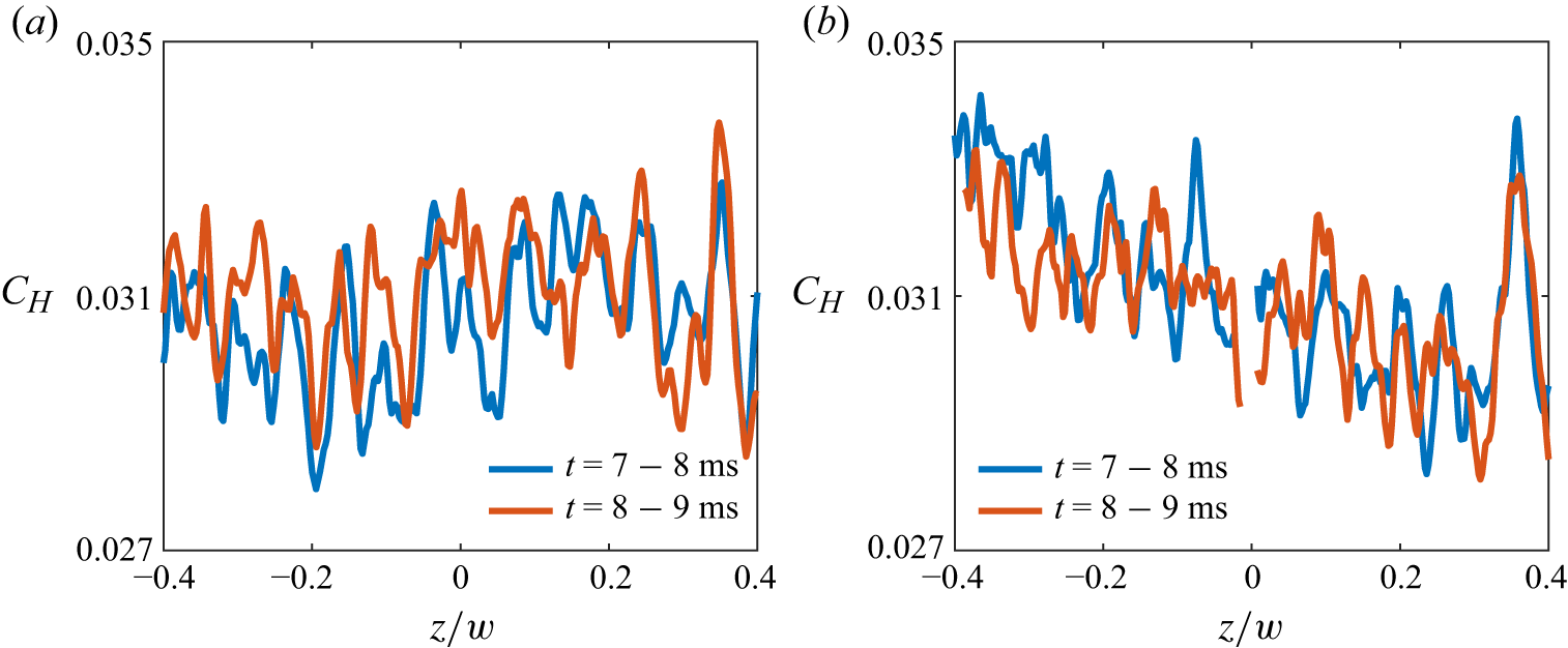
Due to the unsteadiness of heat flux streaks, the heat flux variation along the upstream peak line observed in the time-averaged results is closely related to the selected averaging time range. To illustrate this, figure 19 presents the heat transfer coefficient distributions along the upstream peak line averaged over different time ranges for
 $\chi$
=
 $15^\circ$
and
 $30^\circ$
. The results for the earlier and later portions of the
 $t$
= 7–9 ms interval differ in either the spanwise location or the amplitude of the heat streaks. The results averaged over the entire
 $t$
= 7–9 ms period, shown in figure 8(a), represent a blend between the two, exhibiting a smeared variation in heat flux. Therefore, it can be further inferred that the instantaneous results with a smaller time scale may display more pronounced variations than those shown in the time-averaged result presented here. This phenomenon has also been reported by Roghelia et al. (Reference Roghelia, Olivier, Egorov and Chuvakhov2017).
Standard deviation distributions of the heat transfer coefficient on the ramps; (a–d)
 $\chi$
= 0–45
 $^\circ$
.

Time-averaged heat transfer coefficient distributions along the upstream peak line over different time ranges for the (a)
 $15^\circ$
and (b)
 $30^\circ$
swept ramps.

Appendix D. Heat flux trail near the edge of the ramp’s leading side
In previous experiments on the swept ramp with
 $\alpha$
=
 $34^\circ$
and
 $\chi$
=
 $30^\circ$
, a small fragment of the diaphragm struck the low heat transfer region near
 $z/w = -0.5$
, causing localised minor damage to the paint. This resulted in a trail of increased heat flux downstream of the impact position, as shown in figure 20, consistent with the transition phenomenon triggered by a roughness element in the laminar boundary layer (Tirtey et al. Reference Tirtey, Chazot and Walpot2011; Liu et al. Reference Liu, Wang, Dong, Xia, Chen and Zhao2021). This phenomenon also corroborates the laminar characteristics of the low heat transfer region. It should be noted that this trail also appears in the heat transfer coefficient distribution in figure 5(c), but it is not very clear due to the universal colour bar range. To highlight this interesting detail, the temperature distribution with a suitable colour bar range is provided in figure 20.
Heat flux trail in the low heat transfer region of the ramp with
 $\alpha$
=
 $34^\circ$
and
 $\chi$
=
 $30^\circ$
.