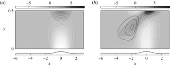
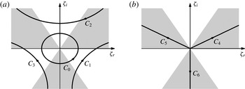
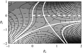
1 Introduction
The introduction of fluid elasticity can fundamentally modify Newtonian flow dynamics. Some examples include the tendency of the polymer to alter the linear amplification of disturbances in shear flows, shift the onset of laminar-to-turbulence transition and reduce drag in the turbulent flow regime. In order to explain the mechanics underpinning some of these flows, there has been recent focus on the transient evolution of idealized disturbances in viscoelastic fluids in both the linear and nonlinear regimes. In the context of such dynamical studies, an important problem is receptivity, and in this work we examine the structure of vortical disturbances generated by surface roughness. The problem set-up is analogous to the Newtonian study by Charru & Hinch (Reference Charru and Hinch2000). We examine the flow response due to small surface undulations on the lower wall of a viscoelastic Couette flow. Our linear analysis demonstrates that elasticity introduces new interesting regimes which differ appreciably from the Newtonian flow.
1.1 The effect of viscoelasticity on flow stability
Viscoelasticity has a profound effect on the stability characteristics of inertia-dominated flows. For example, the temporal growth of inviscid instability waves in mixing layers is attenuated by elasticity, and the amplification of short scales can be suppressed entirely (Azaiez & Homsy Reference Azaiez and Homsy1994). In jets, the interplay between fluid elasticity and flow inertia introduces new modes of instability (Rallison & Hinch Reference Rallison and Hinch1995). Furthermore, spatio-temporal analyses of these flow configurations indicate that viscoelasticity enlarges the region of the parameter space for which these free-shear layers are absolutely unstable (Ray & Zaki Reference Ray and Zaki2014, Reference Ray and Zaki2015). Some of these effects can be understood through an analogy between the elastic normal stress in the shear layer and a membrane tension.
The influence of fluid elasticity on the stability characteristics of moderate Reynolds number, bounded flows has also received attention. In channels, a small amount of elasticity can stabilize the flow with respect to exponential instabilities (Zhang et al. Reference Zhang, Lashgari, Zaki and Brandt2013). The effect of viscoelasticity on non-modal, transient amplification processes was investigated by Hoda, Jovanović & Kumar (Reference Hoda, Jovanović and Kumar2008, Reference Hoda, Jovanović and Kumar2009). Those authors computed the flow response to stochastic body forcing in the momentum equations and demonstrated that the polymer stress fluctuations enhance the associated kinetic energy amplification. In a more recent study, Zhang et al. (Reference Zhang, Lashgari, Zaki and Brandt2013) examined optimal velocity disturbances in channel flows at subcritical Reynolds numbers. A small amount of elasticity strengthens the amplification of streamwise streaks relative to the Newtonian flow, but damps oblique disturbances. The effect of polymer additives on both the lift-up and Orr amplification mechanisms was examined analytically by Page & Zaki (Reference Page and Zaki2014, Reference Page and Zaki2015). For high Weissenberg numbers, two-dimensional vortical disturbances amplify as they align favourably with the shear, which was termed a reverse-Orr effect. The nonlinear stages of the transition process in inertia-dominated viscoelastic channel flow were examined by Agarwal, Brandt & Zaki (Reference Agarwal, Brandt and Zaki2014). They performed direct numerical simulations of subcritical transition initiated by a localized velocity disturbance, and demonstrated that the polymer attenuates the streamwise streaks in the nonlinear regime.
In the above studies the base flows under consideration were parallel, with straight streamlines. In those configurations, the influence of the streamline tension due to the polymer was often stabilizing. In curved geometries, streamline tension has an opposite effect and introduces new elastic instabilities. The most striking feature of these instabilities is their persistence in inertialess flows (Shaqfeh Reference Shaqfeh1996). A combination of experiments and linear stability analyses of an inertialess Taylor–Couette flow identified their physical origin (Muller, Larson & Shaqfeh Reference Muller, Larson and Shaqfeh1989; Larson, Shaqfeh & Muller Reference Larson, Shaqfeh and Muller1990; Shaqfeh, Muller & Larson Reference Shaqfeh, Muller and Larson1992). The viscoelastic inertialess instability depends on the shear rate (Larson et al. Reference Larson, Shaqfeh and Muller1990), and draws energy from the base-state hoop stress in the curved streamlines. A succession of curvature-induced purely elastic instabilities can give way to elastic turbulence – a chaotic state with a broad range of spatial and temporal scales (Groisman & Steinberg Reference Groisman and Steinberg2000).
While there is no inertialess instability in planar viscoelastic Couette flow (Gorodtsov & Leonov Reference Gorodtsov and Leonov1967; Renardy & Renardy Reference Renardy and Renardy1986), parallel viscoelastic flows can exhibit strong non-modal amplification in the zero-Reynolds-number limit (Jovanovic & Kumar Reference Jovanovic and Kumar2010, Reference Jovanovic and Kumar2011; Lieu, Jovanović & Kumar Reference Lieu, Jovanović and Kumar2013; Page & Zaki Reference Page and Zaki2014). In addition, although these flows are asymptotically stable to infinitesimal perturbations, they may be unstable to finite-amplitude disturbances (Morozov & Saarloos Reference Morozov and Saarloos2007). These perturbations induce finite curvature in the streamlines and the flow becomes susceptible to a secondary linear instability (Meulenbroek et al. Reference Meulenbroek, Storm, Morozov and van Saarloos2004; Morozov & Saarloos Reference Morozov and Saarloos2005). There is also experimental evidence that a planar viscoelastic flow can support a self-sustaining chaotic state (Pan et al. Reference Pan, Morozov, Wagner and Arratia2013).
The present study is focused on the manner by which wall undulations induce streamline curvature in parallel viscoelastic shear flows. In low-Reynolds-number Newtonian configurations the flow field is determined by the instantaneous diffusion of vorticity (Charru & Hinch Reference Charru and Hinch2000). As will be demonstrated, the viscoelastic case is richer due to the potential role of the base-state stresses and the wave-like behaviour of vorticity.
1.2 Vorticity wave propagation in viscoelastic fluids
At finite Reynolds numbers the phase difference between the flow and polymer responses provides a mechanism for the propagation of vorticity waves (Joseph Reference Joseph1990). This phenomenon is apparent in the viscoelastic analogues to some of the classical time-dependent solutions of the Navier–Stokes equations. For example, in the starting plate, or Stokes’ first problem, the vortex sheet initiated by the jump in the wall velocity propagates upwards as a shear wave (Tanner Reference Tanner1962; Denn & Porteous Reference Denn and Porteous1971). In oscillatory pipe flows, shear waves can lead to instability (Torralba et al. Reference Torralba, Castrejón-Pita, Hernández, Huelsz, del Río and Ortín2007; Casanellas & Ortín Reference Casanellas and Ortín2014). In micellar solutions, their interference can initiate the formation of shear bands (Zhou, Cook & McKinley Reference Zhou, Cook and Mckinley2012). In wall-bounded flows, vorticity wave propagation and reflection can result in spanwise-travelling re-energizing streaks (Page & Zaki Reference Page and Zaki2014).
The highly tensioned streamlines in a viscoelastic shear flow provide an additional mechanism for wave propagation along the flow direction. Unlike the aforementioned shear waves, these streamwise-travelling waves persist even in dilute solutions. They can lead to new instabilities in flows with shear discontinuities (Rallison & Hinch Reference Rallison and Hinch1995), and the combined effects of wave propagation and shear deformation can amplify disturbances as they align with the shear (Page & Zaki Reference Page and Zaki2015). More fundamentally, the propagation of vorticity waves along tensioned streamlines can introduce critical layers in the flow. Across these layers, the domain is divided into ‘subcritical’ and ‘supercritical’ regions where the fluid is travelling slower and faster than the wave speed, respectively (Joseph, Renardy & Saut Reference Joseph, Renardy and Saut1985). Yoo & Joseph (Reference Yoo and Joseph1985) and Ahrens, Yoo & Joseph (Reference Ahrens, Yoo and Joseph1987) have investigated the change of type which occurs for upper convected Maxwell fluids in channels and pipes with surface waviness. Close to the wall, the vorticity equation is elliptic. There is a sudden change of type at the critical layer, and in the supercritical core of the flow domain the vorticity equation is hyperbolic. This critical layer is smoothed in fluids with a finite solvent viscosity, which are the focus of the current work. However, the critical layers can still have a dramatic influence on the penetration and amplification of vorticity generated at the wavy wall.
The studies by Yoo & Joseph (Reference Yoo and Joseph1985) and Ahrens et al. (Reference Ahrens, Yoo and Joseph1987) focused on the phenomenon of a change in type which occurs in inertia-dominated, instantaneously elastic flows – although they also commented on the form of the perturbation field. For example, Yoo & Joseph (Reference Yoo and Joseph1985) noted that the spanwise-vorticity perturbations induced by the wavy wall are ‘swept out along characteristics’ in the hyperbolic core of the channel, although they could not find an explanation for this property. In the present study, the structure of the vorticity field is explained in detail in terms of the coupling between vorticity and the polymer torque. Detailed asymptotic analyses identify the mechanism for vorticity amplification at the critical layer. Furthermore, we find intriguing behaviour in inertialess flows where the critical layer is outside of the flow domain and does not influence vorticity penetration. The competing effects of the wall wavelength, channel depth, critical layer height, inertia and fluid elasticity are distilled to a dependence on just two parameters: the ratios of the channel depth and of the critical layer height to the roughness wavelength.
The remainder of this paper is organized as follows: in § 2 the physical problem is defined, and the linear perturbation equations are manipulated into a vorticity/polymer-torque system. The various flow regimes are identified and parameterized using a phase diagram in § 3, before the underlying mechanics are explained in § 4. The flow response to localized wall roughness is examined in § 5 and conclusions are provided in § 6.
2 Theoretical formulation
On a macroscopic scale, the presence of small amounts of polymer dissolved in a solvent results in an additional forcing term in the momentum equation due to a polymeric stress,
 ${\it\mu}_{p}F_{i}^{\ast }={\it\mu}_{p}\partial \unicode[STIX]{x1D61B}_{ij}^{\ast }/\partial x_{j}^{\ast }$
. The modified flow equations are
 $$\begin{eqnarray}\displaystyle & \displaystyle \frac{\partial U_{i}^{\ast }}{\partial x_{i}^{\ast }}=0, & \displaystyle\end{eqnarray}$$
 $$\begin{eqnarray}\displaystyle & \displaystyle {\it\rho}\left(\frac{\partial U_{i}^{\ast }}{\partial t^{\ast }}+U_{j}^{\ast }\frac{\partial U_{i}^{\ast }}{\partial x_{j}^{\ast }}\right)=-\frac{\partial P^{\ast }}{\partial x_{i}^{\ast }}+{\it\mu}_{s}\frac{\partial ^{2}U_{i}^{\ast }}{\partial x_{j}^{\ast }\partial x_{j}^{\ast }}+{\it\mu}_{p}F_{i}^{\ast }, & \displaystyle\end{eqnarray}$$
where the asterisk indicates a dimensional variable. The quantities
 ${\it\mu}_{s}$
and
 ${\it\mu}_{p}$
are the dynamic solvent and polymer viscosities, respectively. The current study focuses on dilute solutions, which can be described by the Oldroyd-B model. In an Oldroyd-B fluid, polymer chains are modelled as infinitely extensible dumbbells, and stress is related to the polymer conformation by
 $\unicode[STIX]{x1D61B}_{ij}^{\ast }=(1/{\it\varsigma})(C_{ij}-{\it\delta}_{ij})$
, where
 ${\it\varsigma}$
is the polymer relaxation time. The polymer conformation evolves according to
 $$\begin{eqnarray}\frac{\partial C_{ij}}{\partial t^{\ast }}+U_{k}^{\ast }\frac{\partial C_{ij}}{\partial x_{k}^{\ast }}=C_{ik}\frac{\partial U_{j}^{\ast }}{\partial x_{k}^{\ast }}+C_{jk}\frac{\partial U_{i}^{\ast }}{\partial x_{k}^{\ast }}-\unicode[STIX]{x1D61B}_{ij}^{\ast }.\end{eqnarray}$$
The Oldroyd-B model predicts some of the important behaviours associated with viscoelastic fluids, for example the normal stress difference in shear flows and a fading memory of flow history. In this work, we exploit its simplicity to examine analytically the influence of these effects on the vorticity induced by surface waviness in Couette flow. However, the Oldroyd-B model suffers from well-documented deficiencies, in particular its performance at higher shear rates and failure in extensional flows (Bird, Armstrong & Hassager Reference Bird, Armstrong and Hassager1987). Therefore, in § 5.2, the more realistic FENE-P model, which accounts for the finite extensibility of the polymer chains, is considered numerically.
2.1 The physical problem
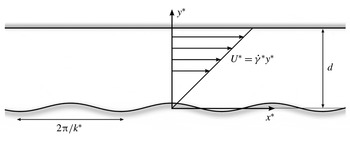
The flow configuration is presented schematically in figure 1. We consider a channel of depth
 $d$
with flow driven by motion of the top plate at speed
 $U_{0}$
. The lower wall has a wavy surface,
 $y^{\ast }=h^{\ast }\text{cos}(k^{\ast }x^{\ast })$
. Under the assumption of small wave slopes,
 ${\it\varepsilon}h\equiv k^{\ast }h^{\ast }\ll 1$
, the flow induced by the surface undulations can be treated as a small
 $O({\it\varepsilon})$
perturbation to a Couette base state,
 $$\begin{eqnarray}U^{\ast }=\dot{{\it\gamma}}^{\ast }y^{\ast },\end{eqnarray}$$
which has an associated constant polymer stress tensor,
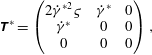 $$\begin{eqnarray}\unicode[STIX]{x1D64F}^{\ast }=\left(\begin{array}{@{}ccc@{}}2\dot{{\it\gamma}}^{\ast 2}{\it\varsigma} & \dot{{\it\gamma}}^{\ast } & 0\\ \dot{{\it\gamma}}^{\ast } & 0 & 0\\ 0 & 0 & 0\end{array}\right),\end{eqnarray}$$
where
 $\dot{{\it\gamma}}^{\ast }\equiv U_{0}/d$
is the shear rate. We consider the problem in a frame where the lower wall is at rest and therefore the perturbations appear steady.
The linearized no-slip condition on the undulating lower wall becomes a slip condition on the perturbation velocity,
 $$\begin{eqnarray}u^{\ast }(x^{\ast },0)=-\dot{{\it\gamma}}^{\ast }h^{\ast }\text{cos}(k^{\ast }x^{\ast }),\quad v^{\ast }(x^{\ast },0)=0,\end{eqnarray}$$
while the perturbation velocities vanish at the upper wall,
 $$\begin{eqnarray}u^{\ast }(x^{\ast },d)=v^{\ast }(x^{\ast },d)=0.\end{eqnarray}$$
The problem is non-dimensionalized by the wavenumber,
 $k^{\ast }$
, and the shear rate,
 $\dot{{\it\gamma}}^{\ast }$
. With this scaling, the base-state velocity profile is
 $U=\dot{{\it\gamma}}y$
, with associated non-dimensional base-state stresses
 $T_{11}=2W\dot{{\it\gamma}}^{2}$
and
 $T_{12}=\dot{{\it\gamma}}$
, where
 $W\equiv \dot{{\it\gamma}}^{\ast }{\it\varsigma}$
is the Weisenberg number, the ratio of the polymer relaxation time to a flow time scale, and the unit dimensionless shear rate
 $\dot{{\it\gamma}}$
is retained for clarity. The equations governing the linear perturbations are now introduced, and are reduced to an Orr–Sommerfeld equation for the streamfunction and an equation for a quantity that plays the role of a polymer potential.
2.2 Linear perturbation equations: streamfunction and polymer potential
For Oldroyd-B fluids, the non-dimensional, steady perturbation equations are
 $$\begin{eqnarray}\displaystyle & \displaystyle \frac{\partial u_{i}^{\prime }}{\partial x_{i}}=0, & \displaystyle\end{eqnarray}$$
 $$\begin{eqnarray}\displaystyle & \displaystyle {\it\Gamma}_{jk}x_{k}\frac{\partial u_{i}^{\prime }}{\partial x_{j}}+u_{j}^{\prime }{\it\Gamma}_{ij}=-\frac{\partial p^{\prime }}{\partial x_{i}}+\frac{{\it\alpha}^{2}}{R}\left({\it\beta}\frac{\partial ^{2}u_{i}^{\prime }}{\partial x_{j}\partial x_{j}}+(1-{\it\beta})f_{i}^{\prime }\right), & \displaystyle\end{eqnarray}$$
 $$\begin{eqnarray}\displaystyle & \displaystyle {\it\Gamma}_{jk}x_{k}\frac{\partial f_{i}^{\prime }}{\partial x_{j}}+\frac{1}{W}f_{i}^{\prime }=f_{j}^{\prime }{\it\Gamma}_{ij}+\unicode[STIX]{x1D61B}_{jk}\frac{\partial ^{2}u_{i}^{\prime }}{\partial x_{j}\partial x_{k}}+\frac{1}{W}\frac{\partial ^{2}u_{i}^{\prime }}{\partial x_{j}\partial x_{j}}, & \displaystyle\end{eqnarray}$$
 ${\it\Gamma}_{ij}$
is the base-state velocity gradient tensor. For Couette flow, the only non-zero entry is
 ${\it\Gamma}_{12}=\dot{{\it\gamma}}(=1)$
. The quantity
 ${\it\alpha}\equiv k^{\ast }d$
is the normalized channel depth,
 $R\equiv \dot{{\it\gamma}}^{\ast }d^{2}/{\it\nu}$
is the bulk Reynolds number and
 ${\it\beta}\equiv {\it\nu}_{s}/{\it\nu}$
is the ratio of the solvent to total viscosity. The variable
 $\boldsymbol{f}^{\prime }\equiv \boldsymbol{{\rm\nabla}}\boldsymbol{\cdot }\boldsymbol{{\it\tau}}^{\prime }$
is the perturbation force due to the polymer (Page & Zaki Reference Page and Zaki2015).
Viscoelastic Couette flow over a wavy wall. The unit length is the inverse wall wavenumber
 $k^{\ast -1}$
; the unit time is the inverse shear rate
 $\dot{{\it\gamma}}^{\ast -1}$
.

Taking the divergence of (2.4c
), we find that the polymer force field is solenoidal,
 $\boldsymbol{{\rm\nabla}}\boldsymbol{\cdot }\boldsymbol{f}^{\prime }=0$
. The present focus on two-dimensional perturbations thus motivates the introduction of the pair of vector potentials for the velocity and polymer force fields,
 $$\begin{eqnarray}\boldsymbol{u}^{\prime }=\boldsymbol{{\rm\nabla}}\wedge {\it\psi}^{\prime }\boldsymbol{e}_{z},\quad \boldsymbol{f}^{\prime }=\boldsymbol{{\rm\nabla}}\wedge {\it\varphi}^{\prime }\boldsymbol{e}_{z},\end{eqnarray}$$
where
 ${\it\psi}^{\prime }$
is the perturbation streamfunction and
 ${\it\varphi}^{\prime }$
is termed the ‘polymer potential’, which is instantaneously tangent to the polymer force vectors (Page & Zaki Reference Page and Zaki2015).
We seek solutions of the form
 $$\begin{eqnarray}\left(\begin{array}{@{}c@{}}{\it\psi}^{\prime }(\boldsymbol{x})\\ {\it\varphi}^{\prime }(\boldsymbol{x})\end{array}\right)=\text{Re}\left\{\left(\begin{array}{@{}c@{}}{\it\psi}(y)\\ {\it\varphi}(y)\end{array}\right)\text{e}^{\text{i}kx}\right\},\end{eqnarray}$$
where the unit non-dimensional wavenumber,
 $k=1$
, is retained for clarity, and manipulate equations (2.4) into a viscoelastic Orr–Sommerfeld system,
 $$\begin{eqnarray}\displaystyle & \displaystyle \text{i}k\dot{{\it\gamma}}y\left(\frac{\text{d}^{2}}{\text{d}y^{2}}-k^{2}\right){\it\psi}=\frac{{\it\alpha}^{2}}{R}\left[{\it\beta}\left(\frac{\text{d}^{2}}{\text{d}y^{2}}-k^{2}\right)^{2}{\it\psi}+(1-{\it\beta})\left(\frac{\text{d}^{2}}{\text{d}y^{2}}-k^{2}\right){\it\varphi}\right], & \displaystyle\end{eqnarray}$$
 $$\begin{eqnarray}\displaystyle & \displaystyle \text{i}k\dot{{\it\gamma}}y{\it\varphi}+\frac{1}{W}{\it\varphi}=\left[-k^{2}T_{11}+2\text{i}kT_{12}\frac{\text{d}}{\text{d}y}+\frac{1}{W}\left(\frac{\text{d}^{2}}{\text{d}y^{2}}-k^{2}\right)\right]{\it\psi}. & \displaystyle\end{eqnarray}$$
 $$\begin{eqnarray}\text{d}_{y}{\it\psi}(0)=-\dot{{\it\gamma}}h,\quad {\it\psi}(0)=0,\end{eqnarray}$$
where
 $h=1$
is assumed such that the wave slope is a small parameter,
 ${\it\varepsilon}h=k^{\ast }h^{\ast }$
. The streamfunction and its gradient have homogeneous boundary conditions at the top wall,
 $y={\it\alpha}$
.
It will often be instructive to analyse the perturbation field in terms of the spanwise vorticity,
 ${\it\omega}\equiv -{\rm\nabla}^{2}{\it\psi}=-(\text{d}_{y}^{2}-k^{2}){\it\psi}$
, and the spanwise polymer torque,
 ${\it\chi}\equiv -{\rm\nabla}^{2}{\it\varphi}=-(\text{d}_{y}^{2}-k^{2}){\it\varphi}$
, which are governed by
 $$\begin{eqnarray}\displaystyle & \displaystyle \text{i}k\dot{{\it\gamma}}y{\it\omega}=\frac{{\it\alpha}^{2}}{R}\left[{\it\beta}\left(\frac{\text{d}^{2}}{\text{d}y^{2}}-k^{2}\right){\it\omega}+(1-{\it\beta}){\it\chi}\right], & \displaystyle\end{eqnarray}$$
 $$\begin{eqnarray}\displaystyle & \displaystyle \text{i}k\dot{{\it\gamma}}y{\it\chi}+\frac{1}{W}{\it\chi}=2\text{i}k\dot{{\it\gamma}}\frac{\text{d}{\it\varphi}}{\text{d}y}+\left[-k^{2}T_{11}+2\text{i}kT_{12}\frac{\text{d}}{\text{d}y}+\frac{1}{W}\left(\frac{\text{d}^{2}}{\text{d}y^{2}}-k^{2}\right)\right]{\it\omega}. & \displaystyle\end{eqnarray}$$
3 Flow regimes and phase diagram
3.1 Quasi-Newtonian flow
Here we briefly examine the flow response to the surface waviness in the low-Weissenberg-number limit. This limit yields a quasi-Newtonian behaviour, and at leading order, the results are identical to those presented by Charru & Hinch (Reference Charru and Hinch2000). Therefore, this section establishes the background against which the elasticity-dominated flows are compared in subsequent sections.
In the limit of small Weissenberg number,
 $W\ll 1$
, the polymer behaves like an additional solvent. To leading order in
 $W$
, the equations for the vorticity (2.9a
) and polymer torque (2.9b
) are
 $$\begin{eqnarray}\displaystyle & \displaystyle \text{i}k\dot{{\it\gamma}}y{\it\omega}_{0}=\frac{{\it\alpha}^{2}}{R}\left[{\it\beta}\left(\frac{\text{d}^{2}}{\text{d}y^{2}}-k^{2}\right){\it\omega}_{0}+(1-{\it\beta}){\it\chi}_{0}\right], & \displaystyle\end{eqnarray}$$
 $$\begin{eqnarray}\displaystyle & \displaystyle {\it\chi}_{0}=\left(\frac{\text{d}^{2}}{\text{d}y^{2}}-k^{2}\right){\it\omega}_{0}. & \displaystyle\end{eqnarray}$$
 ${\it\chi}_{0}$
depends on the curvature in the vorticity field alone. The Newtonian spanwise vorticity is recovered after combining the system (3.1),
 $$\begin{eqnarray}\text{i}k\dot{{\it\gamma}}y{\it\omega}_{0}=\frac{{\it\alpha}^{2}}{R}\left(\frac{\text{d}^{2}}{\text{d}y^{2}}-k^{2}\right){\it\omega}_{0}.\end{eqnarray}$$
An identical equation is obtained in the limit of pure solvent,
 ${\it\beta}=1$
.
The solution to equation (3.2) above a wavy wall was discussed in detail by Charru & Hinch (Reference Charru and Hinch2000). Those authors demonstrated that the vorticity perturbations induced by the lower wall can be classified into three regimes, depending on the values of a pair of parameters:
 $$\begin{eqnarray}{\it\alpha}\equiv k^{\ast }d\quad \text{and}\quad {\it\theta}\equiv \left(\frac{{\it\alpha}^{2}}{R}\right)^{1/3}=\left(\frac{{\it\nu}k^{\ast 2}}{\dot{{\it\gamma}}^{\ast }}\right)^{1/3}.\end{eqnarray}$$
The first of these,
 ${\it\alpha}$
, is the normalized channel depth. The second,
 ${\it\theta}$
, is a normalized viscous length scale. Three regimes are defined following the analysis and terminology introduced by Charru & Hinch (Reference Charru and Hinch2000): (i) the shallow-viscous regime,
 ${\it\alpha}<1$
;
 ${\it\theta}>{\it\alpha}$
; (ii) the deep-viscous regime,
 ${\it\alpha}>1$
,
 ${\it\theta}>1$
; (iii) the inviscid regime,
 ${\it\alpha}>1$
,
 ${\it\theta}<1$
.
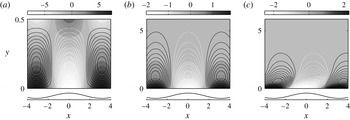
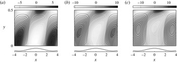
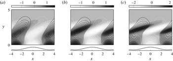
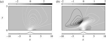
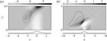
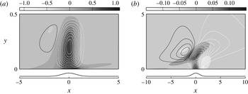
Vortical perturbations (top) induced by the wavy wall (bottom) in Newtonian fluids. Filled contours are the spanwise vorticity, lines are the streamfunction. (a) Shallow-viscous regime
 ${\it\alpha}=0.5$
and
 ${\it\theta}=0.63$
. (b) Deep-viscous regime,
 ${\it\alpha}=10$
and
 ${\it\theta}=4.64$
. (c) Inviscid regime,
 ${\it\alpha}=10$
and
 ${\it\theta}=0.46$
.

The vorticity and streamfunction in three examples representative of the Newtonian regimes are reported in figure 2. In figure 2(a) the vorticity perturbation fills the channel and the effects of inertia, which would tip the roll structures forward with the shear, are negligible. This behaviour is characteristic of the shallow-viscous regime where the roughness wavelength is longer than the channel depth,
 ${\it\alpha}<1$
, and the viscous length is greater than the channel height,
 ${\it\theta}>{\it\alpha}$
. In figure 2(b), the vorticity perturbations penetrate about a wavelength into the flow and inertial effects are still unimportant. This behaviour, which occurs for deep channels,
 ${\it\alpha}>1$
, with
 ${\it\theta}>1$
, is termed the ‘deep-viscous’ regime. Finally, figure 2(c) is an example of the ‘inviscid regime’. The induced rolls are tipped forward under the action of the shear, while the vorticity penetration depth is of the order of the viscous length. This regime is associated with conditions where
 ${\it\alpha}>1$
and
 ${\it\theta}<1$
.
In order to quantify vorticity penetration, Charru & Hinch (Reference Charru and Hinch2000) introduced a measure of penetration depth based on the inverse wall vorticity,
 $|{\it\omega}(0)|^{-1}$
. This definition is intuitive because the action of viscous diffusion means that the vorticity maximum is always at the lower wall, and in deep channels vorticity monotonically decays with increasing
 $y$
. Elasticity-dominated flows with
 $W>1$
do not share these Newtonian characteristics, and a more general definition of penetration depth will be required.
3.2 Viscoelastic phase diagram
Similar to the quasi-Newtonian limit, the solution at moderate to high Weissenberg numbers depends on two dimensionless parameters. The first remains the normalized channel depth,
 ${\it\alpha}\equiv k^{\ast }d$
. However, the viscous diffusion length is now of secondary importance. We will see that vorticity penetration is instead dependent on the parameter,
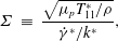 $$\begin{eqnarray}\displaystyle {\it\Sigma} & \equiv & \displaystyle \frac{\sqrt{{\it\mu}_{p}T_{11}^{\ast }/{\it\rho}}}{\dot{{\it\gamma}}^{\ast }/k^{\ast }},\end{eqnarray}$$
 $$\begin{eqnarray}\displaystyle & = & \displaystyle \frac{\sqrt{2{\it\nu}_{p}{\it\varsigma}}}{1/k^{\ast }},\end{eqnarray}$$
 $E^{\ast }\equiv (1-{\it\beta})W/R$
, by
 ${\it\Sigma}=k^{\ast }d\sqrt{E^{\ast }}$
. However, when written in the form (3.4a
),
 ${\it\Sigma}$
may be interpreted as the ratio of a vorticity wave speed,
 $c_{{\it\omega}}^{\ast }=\sqrt{{\it\mu}_{p}T_{11}^{\ast }/{\it\rho}}$
, to the base-flow velocity one wavelength above the lower wall. This classification reflects that vorticity fluctuations in a viscoelastic flow may propagate as streamwise-travelling waves along the tensioned mean-flow streamlines – a scenario which shares some similarities with the propagation of Alfvén waves along magnetic field lines (Chandrasekhar Reference Chandrasekhar1961). The difference in the viscoelastic case is that a mean shear is required to establish the normal stress
 ${\it\mu}_{p}T_{11}^{\ast }$
, and this shearing also has associated with it a kinematic vorticity amplification mechanism (Page & Zaki Reference Page and Zaki2015). When written in the form (3.4b
),
 ${\it\Sigma}$
is a ratio of length scales: the critical layer height and the roughness wavelength. The critical layer is the surface where the speed of the base flow matches the wave speed
 $c_{{\it\omega}}^{\ast }$
. While the vorticity perturbations are steady in the present problem, the longitudinal vorticity wave speed
 $c_{{\it\omega}}^{\ast }$
remains an important property of the viscolelastic flow. The critical layer height, which can be thought of as the point where an observer travelling with the mean flow would see the lower wall disturbance sweep by at the elastic wave speed, has particular physical significance (§ 4.3).
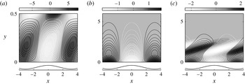
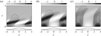
Vortical perturbations (top) induced by the wavy wall (bottom). Filled contours are the spanwise vorticity, lines are the streamfunction. (a) Shallow-elastic regime
 ${\it\alpha}=0.5$
and
 ${\it\Sigma}=3$
with
 $R=1$
,
 ${\it\beta}=0.7$
,
 $W=60$
. (b) Deep-elastic regime,
 ${\it\alpha}=10$
and
 ${\it\Sigma}=60$
with
 $R=1$
,
 ${\it\beta}=0.7$
,
 $W=60$
. (c) Transcritical regime,
 ${\it\alpha}=10$
and
 ${\it\Sigma}=1.9$
with
 $R=1000$
,
 ${\it\beta}=0.7$
,
 $W=60$
.

Three examples of vortical disturbances induced by the lower wall in flows with a fairly large Weissenberg number,
 $W=60$
, are reported in figure 3. The same behaviour is preserved at lower values of
 $W$
, but a relatively high value was adopted here in order to highlight the observed effects. Each of the panels in the figure illustrates a different regime.
In figure 3(a) counter-rotating rolls fill the channel. Rolls with positive vorticity sit above troughs and with negative vorticity over peaks. The parameters correspond to the shallow-viscous behaviour in a Newtonian fluid. However, in this high-Weissenberg-number flow, the rolls are tipped forward, a behaviour normally attributed to inertial effects. In addition, the vorticity maxima are located along the top wall. In general, these characteristics are associated with conditions where
 ${\it\alpha}\lesssim 1$
,
 ${\it\Sigma}>{\it\alpha}$
which we term ‘shallow-elastic’ flows.
In figure 3(b), the rolls remain in phase with the surface waviness and their associated vorticity decays within roughly one wavelength from the wall. Despite the high Weissenberg number, the perturbation flow is indistinguishable from the Newtonian deep-viscous regime. In general, this behaviour occurs when
 ${\it\alpha}\gtrsim 1$
and
 ${\it\Sigma}\gtrsim 1$
, and is denoted the ‘deep-elastic’ regime.
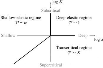
Finally, the most intriguing behaviour is encountered when
 ${\it\alpha}>{\it\Sigma}$
and
 ${\it\Sigma}\lesssim 1$
, and is displayed in figure 3(c). The vorticity is amplified in stripes tilted forward with the shear, and the amplification is localized around a
 $y$
-location away from the wall. This regime is referred to as ‘transcritical’ flow.
Both the shallow-elastic and transcritical flows have characteristics which differ substantially from the Newtonian configuration. Shallow-elastic flows exhibit vorticity amplification at the upper wall, while flows in the transcritical regime are characterized by non-local vorticity amplification in the bulk of the channel. These features motivate a definition of penetration depth based on a measure of the total perturbation vorticity, rather than one constructed from local information about the vorticity magnitude. We adopt the following measure of penetration depth,
 $$\begin{eqnarray}{\mathcal{P}}\equiv y({\it\Lambda}^{r}=0.99);\quad \text{where }{\it\Lambda}^{r}(y)=\frac{\displaystyle \int _{0}^{y}|{\it\omega}(y^{\prime })|^{2}\,\text{d}y^{\prime }}{\displaystyle \int _{0}^{{\it\alpha}}|{\it\omega}(y^{\prime })|^{2}\,\text{d}y^{\prime }},\end{eqnarray}$$
which can account for non-local effects. Note that (3.5) recovers the Newtonian scalings for penetration depth found by Charru & Hinch (Reference Charru and Hinch2000) in the limit
 $W\ll 1$
.
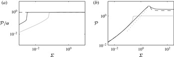
Penetration depth,
 ${\mathcal{P}}$
as a function of
 ${\it\Sigma}$
. (a) ‘Shallow’ channels with
 $W=60$
,
 ${\it\beta}=0.7$
: dashed line,
 ${\it\alpha}=0.01$
; black solid line,
 ${\it\alpha}=0.1$
; grey solid line,
 ${\it\alpha}=0.5$
. (b) ‘Deep’ channels with
 $W=60$
,
 ${\it\beta}=0.7$
; grey solid line,
 ${\it\alpha}=1$
; black solid line,
 ${\it\alpha}=5$
; dashed line,
 ${\it\alpha}=10$
. The dotted line is
 ${\mathcal{P}}={\it\Sigma}$
.

Phase diagram for vorticity disturbances initiated by the surface waviness.

The penetration depth
 ${\mathcal{P}}$
is evaluated for a range of
 ${\it\alpha}$
and
 ${\it\Sigma}$
and is used in figure 4 to examine the transitions between the three regimes reported in figure 3. Shallow channels,
 ${\it\alpha}<1$
, are considered in figure 4(a) and
 ${\it\Sigma}$
(or the vorticity wave speed) is varied by changing the bulk Reynolds number,
 $R$
. When the critical layer is outside of the flow domain,
 ${\it\Sigma}\gtrsim {\it\alpha}$
, the vorticity perturbation fills the channel,
 ${\mathcal{P}}\sim {\it\alpha}$
. Deep channels are considered in figure 4(b). When
 ${\it\Sigma}\lesssim 1$
the penetration depth scales with the dimensionless critical layer height,
 ${\mathcal{P}}\sim {\it\Sigma}$
(transcritical regime). There is a sharp transition to the deep-elastic regime when
 ${\it\Sigma}\gtrsim 1$
and penetration is of the order of a wavelength,
 ${\mathcal{P}}\sim 1$
.
In analogy to the Newtonian problem (Charru & Hinch Reference Charru and Hinch2000), these results may be summarized in the form of a ‘phase diagram’. The diagram for the viscoelastic Couette flow is presented schematically in figure 5. Each of the three regimes spans a sector in the
 $\{\log {\it\alpha},\log {\it\Sigma}\}$
plane. This classification does not explain the characteristics of the vorticity eigenfunctions in each regime; for example the vorticity generation at the top wall in shallow-elastic flows or the amplification of vorticity in the bulk fluid in transcritical channels. These effects are now explored further using asymptotic analyses.
4 Asymptotic solutions in the three regimes
4.1 Shallow-elastic flow
Shallow-elastic flows are those where
 ${\it\alpha}\lesssim 1$
and
 ${\it\Sigma}>{\it\alpha}$
. The second of these criteria means that the base flow is slower than the vorticity wave speed; the critical layer is outside of the flow domain. Examples of the streamfunction and vorticity in this regime are provided in figure 6 for increasing values of the Weissenberg number,
 $W$
. As
 $W$
is increased, the vorticity across the bulk of the channel becomes nearly constant, except for a rapid variation close to the upper wall where it is significantly amplified. This behaviour should be contrasted with Newtonian shallow-viscous flows where the vorticity distribution is linear and dictated by viscous diffusion.
Vortical perturbations (top) induced by the wavy wall (bottom) in the shallow-elastic regime. Filled contours are the spanwise vorticity, lines are the streamfunction. The channel depth
 ${\it\alpha}=0.5$
, and the solvent viscosity and bulk Reynolds numbers are fixed,
 $R=1$
,
 ${\it\beta}=0.5$
. (a)
 $W=20$
(
 ${\it\Sigma}=2.24$
); (b)
 $W=40$
(
 ${\it\Sigma}=3.16$
); (c)
 $W=80$
(
 ${\it\Sigma}=4.47$
).

In order to explain the structure of the vorticity perturbation in this regime, we examine the streamfunction–polymer potential system (2.7) in the long-wave limit,
 ${\it\alpha}\ll 1$
. The solution to the long-wave equations will be shown to depend on the parameter
 ${\mathcal{W}}\equiv {\it\alpha}\dot{{\it\gamma}}W$
. In the limit
 ${\mathcal{W}}\gg 1$
the bulk flow response to the vorticity injection at the bottom wall can be classified as ‘elastic’, and a solvent boundary layer forms at the upper wall where the spanwise vorticity is amplified by a factor which we will show is
 ${\mathcal{W}}^{1/2}$
.
The present interest in shallow channels motivates rescaling the equations by the channel height
 $Y=y/{\it\alpha}$
, with
 ${\it\alpha}^{2}\hat{{\it\psi}}(Y)={\it\psi}(y)$
,
 $\hat{{\it\varphi}}(Y)={\it\varphi}(y)$
. The system of (2.7) becomes
 $$\begin{eqnarray}\displaystyle & \displaystyle \text{i}{\it\alpha}\dot{{\it\gamma}}Y\left(\frac{\text{d}^{2}}{\text{d}Y^{2}}-{\it\alpha}^{2}\right)\hat{{\it\psi}}=\frac{{\it\beta}}{R}\left(\frac{\text{d}^{2}}{\text{d}Y^{2}}-{\it\alpha}^{2}\right)^{2}\hat{{\it\psi}}+\frac{(1-{\it\beta})}{R}\left(\frac{\text{d}^{2}}{\text{d}Y^{2}}-{\it\alpha}^{2}\right)\hat{{\it\varphi}}, & \displaystyle\end{eqnarray}$$
 $$\begin{eqnarray}\displaystyle & \displaystyle \left(Y+\frac{1}{\text{i}{\mathcal{W}}}\right)\hat{{\it\varphi}}=\left[2\text{i}{\mathcal{W}}+2\frac{\text{d}}{\text{d}Y}+\frac{1}{\text{i}{\mathcal{W}}}\left(\frac{\text{d}^{2}}{\text{d}Y^{2}}-{\it\alpha}^{2}\right)\right]\hat{{\it\psi}}, & \displaystyle\end{eqnarray}$$
 ${\mathcal{W}}\equiv {\it\alpha}\dot{{\it\gamma}}W=U_{0}{\it\varsigma}k^{\ast }$
is proportional to the number of bottom waves that an observer travelling at the top wall speed would pass in a relaxation time
 ${\it\varsigma}$
. Assuming that
 ${\it\alpha}\ll 1$
, an expansion in powers of
 ${\it\alpha}^{-1}$
yields the leading-order equations,
 $$\begin{eqnarray}\displaystyle & \displaystyle 0={\it\beta}\frac{\text{d}^{4}\hat{{\it\psi}}_{0}}{\text{d}Y^{4}}+(1-{\it\beta})\frac{\text{d}^{2}\hat{{\it\varphi}}_{0}}{\text{d}Y^{2}}, & \displaystyle\end{eqnarray}$$
 $$\begin{eqnarray}\displaystyle & \displaystyle \left(Y+\frac{1}{\text{i}{\mathcal{W}}}\right)\hat{{\it\varphi}}_{0}=\left(2\text{i}{\mathcal{W}}+2\frac{\text{d}}{\text{d}Y}+\frac{1}{\text{i}{\mathcal{W}}}\frac{\text{d}^{2}}{\text{d}Y^{2}}\right)\hat{{\it\psi}}_{0}. & \displaystyle\end{eqnarray}$$
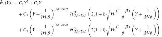 $$\begin{eqnarray}\displaystyle \hat{{\it\psi}}_{0}(Y) & = & \displaystyle C_{1}Y^{2}+C_{2}Y\nonumber\\ \displaystyle & & \displaystyle +\,C_{3}\left(Y+\frac{1}{\text{i}{\mathcal{W}}{\it\beta}}\right)^{(3{\it\beta}-2)/2{\it\beta}}{\mathcal{H}}_{(3{\it\beta}-2)/{\it\beta}}^{(1)}\left(2(1+\text{i})\sqrt{{\mathcal{W}}\frac{(1-{\it\beta})}{{\it\beta}}\left(Y+\frac{1}{\text{i}{\mathcal{W}}{\it\beta}}\right)}\right)\nonumber\\ \displaystyle & & \displaystyle +\,C_{4}\left(Y+\frac{1}{\text{i}{\mathcal{W}}{\it\beta}}\right)^{(3{\it\beta}-2)/2{\it\beta}}{\mathcal{H}}_{(3{\it\beta}-2)/{\it\beta}}^{(2)}\left(2(1+\text{i})\sqrt{{\mathcal{W}}\frac{(1-{\it\beta})}{{\it\beta}}\left(Y+\frac{1}{\text{i}{\mathcal{W}}{\it\beta}}\right)}\right),\nonumber\\ \displaystyle & & \displaystyle\end{eqnarray}$$
where the
 ${\mathcal{H}}_{n}^{(j)}$
are Hankel functions of order
 $n$
. The solution is a function of
 ${\mathcal{W}}$
and the polymer concentration,
 ${\it\beta}$
. However, extracting the physical mechanism behind the vorticity amplification from this solution is difficult. Since the upper wall amplification is increasingly pronounced for large
 ${\mathcal{W}}$
, we instead seek an approximate solution of the long-wave equations (4.2) assuming
 ${\mathcal{W}}\gg 1$
.
Bulk elastic solution: defining
 ${\it\varepsilon}\equiv {\mathcal{W}}^{-1}\ll 1$
and
 $\hat{{\it\Phi}}_{0}={\it\varepsilon}\hat{{\it\varphi}}_{0}$
, equations (4.2) become
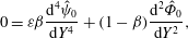 $$\begin{eqnarray}\displaystyle & \displaystyle 0={\it\varepsilon}{\it\beta}\frac{\text{d}^{4}\hat{{\it\psi}}_{0}}{\text{d}Y^{4}}+(1-{\it\beta})\frac{\text{d}^{2}\hat{{\it\Phi}}_{0}}{\text{d}Y^{2}}, & \displaystyle\end{eqnarray}$$
 $$\begin{eqnarray}\displaystyle & \displaystyle (Y-\text{i}{\it\varepsilon})\hat{{\it\Phi}}_{0}=\bigg(\underbrace{\vphantom{\frac{\text{d}}{\text{d}Y}}2\text{i}}_{}+\underbrace{2{\it\varepsilon}\frac{\text{d}}{\text{d}Y}}_{}-\text{i}{\it\varepsilon}^{2}\frac{\text{d}^{2}}{\text{d}Y^{2}}\bigg)\hat{{\it\psi}}_{0}, & \displaystyle\end{eqnarray}$$
 $T_{11}$
and
 $T_{12}$
(cf. equation 2.7b
). We adopt the asymptotic expansion
 $$\begin{eqnarray}\displaystyle & \displaystyle \hat{{\it\psi}}_{0}(Y;{\it\varepsilon}) & \displaystyle =\hat{{\it\psi}}_{0}^{0}(Y)+{\it\varepsilon}^{1/2}\hat{{\it\psi}}_{0}^{1/2}(Y)+{\it\varepsilon}\hat{{\it\psi}}_{0}^{1}(Y)+\cdots ,\end{eqnarray}$$
 $$\begin{eqnarray}\displaystyle & \displaystyle \hat{{\it\Phi}}_{0}(Y;{\it\varepsilon}) & \displaystyle =\hat{{\it\Phi}}_{0}^{0}(Y)+\underbrace{{\it\varepsilon}^{1/2}\hat{{\it\Phi}}_{0}^{1/2}(Y)}_{}+{\it\varepsilon}\hat{{\it\Phi}}_{0}^{1}(Y)+\cdots ,\end{eqnarray}$$
 $O({\it\varepsilon}^{1/2})$
, identified with an underbrace, will be required for matching with the solution at the top wall.
At leading order and
 $O({\it\varepsilon}^{1/2})$
,
 $$\begin{eqnarray}\displaystyle & \displaystyle 0=\frac{\text{d}^{2}\hat{{\it\Phi}}_{0}^{j}}{\text{d}Y^{2}}, & \displaystyle\end{eqnarray}$$
 $$\begin{eqnarray}\displaystyle & \displaystyle Y\hat{{\it\Phi}}_{0}^{j}=2\text{i}\hat{{\it\psi}}_{0}^{j}. & \displaystyle\end{eqnarray}$$
 $\hat{{\it\chi}}_{0}\propto -\text{d}_{Y}^{2}\hat{{\it\Phi}}_{0}$
, is zero to leading order. Equation (4.6b
) indicates that forces are generated through the action of the base-state streamwise stress on curvature in the perturbation streamlines as the polymer is advected. After applying the boundary conditions at
 $Y=0$
we find
 $$\begin{eqnarray}\hat{{\it\psi}}_{0}^{0}(Y)=Y(A_{0}Y-{\hat{h}}),\quad \hat{{\it\psi}}_{0}^{1/2}(Y)=A_{1/2}Y^{2},\end{eqnarray}$$
where
 $A_{0}$
and
 $A_{1/2}$
are constants and
 ${\hat{h}}\equiv h/{\it\alpha}$
. The first-order correction accounts for polymer relaxation and also the influence of the base-state shear stress,
 $T_{12}$
,
 $$\begin{eqnarray}\displaystyle & \displaystyle 0=\frac{\text{d}^{2}\hat{{\it\Phi}}_{0}^{1}}{\text{d}Y^{2}}, & \displaystyle\end{eqnarray}$$
 $$\begin{eqnarray}\displaystyle & \displaystyle Y\hat{{\it\Phi}}_{0}^{1}-\text{i}\hat{{\it\Phi}}_{0}^{0}=2\text{i}\hat{{\it\psi}}_{0}^{1}-2\frac{\text{d}\hat{{\it\psi}}_{0}^{0}}{\text{d}Y}. & \displaystyle\end{eqnarray}$$
 $Y=0$
, the streamfunction is
 $\hat{{\it\psi}}_{0}^{1}(Y)=A_{1}Y^{2}$
, and the solution correct to
 $O({\it\varepsilon})$
reads
 $$\begin{eqnarray}\hat{{\it\psi}}_{0}(Y)=Y(A_{0}Y-{\hat{h}})+{\it\varepsilon}^{1/2}A_{1/2}Y^{2}+{\it\varepsilon}A_{1}Y^{2}+\cdots .\end{eqnarray}$$
This expression, which is dictated by elastic effects only, corresponds to a vorticity perturbation which is constant across the channel,
 ${\it\omega}_{0}(Y)=-2A_{0}-2{\it\varepsilon}^{1/2}A_{1/2}-\cdots .$
In fact, the elastic flow response (4.9) is a simple distortion of the mean-flow streamlines to mimic the topography of the lower wall across the depth of the channel. As such, it cannot satisfy both boundary conditions at the upper wall,
 $Y=1$
.
Upper wall layer: in order to focus on the upper wall region, we introduce the new coordinate
 ${\it\eta}\equiv (Y-1)/{\it\delta}({\it\varepsilon})$
. In terms of
 ${\it\eta}$
, the bulk streamfunction (4.9) takes the form
 $$\begin{eqnarray}\hat{{\it\psi}}_{0}({\it\eta})=A_{0}-{\hat{h}}+{\it\varepsilon}^{1/2}[(2A_{0}-{\hat{h}}){\it\eta}+A_{1/2}]+{\it\varepsilon}(A_{0}{\it\eta}^{2}+2A_{1/2}{\it\eta}+A_{1})+\cdots .\end{eqnarray}$$
Enforcing the no penetration condition at
 $Y=1$
, or
 ${\it\eta}=0$
, implies
 $A_{0}={\hat{h}}$
. There is a non-zero gradient in the streamfunction, or a slip velocity, which must be corrected by the inner solution.
In the wall layer, we define the vorticity and polymer potential,
 $\{\overline{{\it\psi}}_{0}({\it\eta}),\overline{{\it\Phi}}_{0}({\it\eta})\}=\{\hat{{\it\psi}}_{0}(Y),\hat{{\it\Phi}}_{0}(Y)\}$
, and the rescaled equations (4.2) become,
 $$\begin{eqnarray}\displaystyle & \displaystyle 0={\it\varepsilon}{\it\beta}\frac{\text{d}^{4}\overline{{\it\psi}}_{0}}{\text{d}{\it\eta}^{4}}+{\it\delta}^{2}(1-{\it\beta})\frac{\text{d}^{2}\overline{{\it\Phi}}_{0}}{\text{d}{\it\eta}^{2}}, & \displaystyle\end{eqnarray}$$
 $$\begin{eqnarray}\displaystyle & \displaystyle (1+{\it\delta}{\it\eta}-\text{i}{\it\varepsilon})\overline{{\it\Phi}}_{0}=\left(2\text{i}+2\frac{{\it\varepsilon}}{{\it\delta}}\frac{\text{d}}{\text{d}{\it\eta}}-\frac{\text{i}{\it\varepsilon}^{2}}{{\it\delta}^{2}}\frac{\text{d}^{2}}{\text{d}{\it\eta}^{2}}\right)\overline{{\it\psi}}_{0}. & \displaystyle\end{eqnarray}$$
 ${\it\delta}={\it\varepsilon}^{1/2}$
, which motivates the asymptotic expansion,
 $$\begin{eqnarray}\displaystyle & \displaystyle \overline{{\it\psi}}_{0}({\it\eta};{\it\varepsilon})={\it\varepsilon}^{1/2}(\overline{{\it\psi}}_{0}^{0}({\it\eta})+{\it\varepsilon}^{1/2}\overline{{\it\psi}}_{0}^{1}({\it\eta})+\cdots \,), & \displaystyle\end{eqnarray}$$
 $$\begin{eqnarray}\displaystyle & \displaystyle \overline{{\it\Phi}}_{0}({\it\eta};{\it\varepsilon})={\it\varepsilon}^{1/2}(\overline{{\it\Phi}}_{0}^{0}({\it\eta})+{\it\varepsilon}^{1/2}\overline{{\it\Phi}}_{0}^{1}({\it\eta})+\cdots \,). & \displaystyle\end{eqnarray}$$
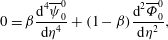 $$\begin{eqnarray}\displaystyle & \displaystyle 0={\it\beta}\frac{\text{d}^{4}\overline{{\it\psi}}_{0}^{0}}{\text{d}{\it\eta}^{4}}+(1-{\it\beta})\frac{\text{d}^{2}\overline{{\it\Phi}}_{0}^{0}}{\text{d}{\it\eta}^{2}}, & \displaystyle\end{eqnarray}$$
 $$\begin{eqnarray}\displaystyle & \displaystyle \overline{{\it\Phi}}_{0}^{0}=2\text{i}\overline{{\it\psi}}_{0}^{0}. & \displaystyle\end{eqnarray}$$
 ${\it\eta}\rightarrow -\infty$
and applying the homogeneous boundary conditions at
 ${\it\eta}=0$
, the leading-order streamfunction is
 $$\begin{eqnarray}\overline{{\it\psi}}_{0}^{0}({\it\eta})=\overline{B}_{0}({\it\kappa}{\it\eta}+1-\text{e}^{{\it\kappa}{\it\eta}}),\end{eqnarray}$$
where
 ${\it\kappa}=(1-\text{i})\sqrt{(1-{\it\beta})/{\it\beta}}$
. At first order there are correction terms due to advection of the polymer and the base shear stress
 $T_{12}$
,
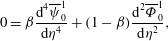 $$\begin{eqnarray}\displaystyle & \displaystyle 0={\it\beta}\frac{\text{d}^{4}\overline{{\it\psi}}_{0}^{1}}{\text{d}{\it\eta}^{4}}+(1-{\it\beta})\frac{\text{d}^{2}\overline{{\it\Phi}}_{0}^{1}}{\text{d}{\it\eta}^{2}}, & \displaystyle\end{eqnarray}$$
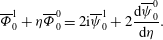 $$\begin{eqnarray}\displaystyle & \displaystyle \overline{{\it\Phi}}_{0}^{1}+{\it\eta}\overline{{\it\Phi}}_{0}^{0}=2\text{i}\overline{{\it\psi}}_{0}^{1}+2\frac{\text{d}\overline{{\it\psi}}_{0}^{0}}{\text{d}{\it\eta}}. & \displaystyle\end{eqnarray}$$
 $\overline{{\it\psi}}_{0}^{1}$
, the inner streamfunction to
 $O({\it\varepsilon})$
is
 $$\begin{eqnarray}\displaystyle \overline{{\it\psi}}_{0}({\it\eta}) & = & \displaystyle {\it\varepsilon}^{1/2}\overline{B}_{0}({\it\kappa}{\it\eta}+1-\text{e}^{{\it\kappa}{\it\eta}})\nonumber\\ \displaystyle & & \displaystyle +\,{\it\varepsilon}\left[\overline{B}_{1}({\it\kappa}{\it\eta}+1-\text{e}^{{\it\kappa}{\it\eta}})+\overline{B}_{0}\left({\it\kappa}{\it\eta}^{2}-\frac{(2\text{i}{\it\kappa}^{2}-1){\it\eta}}{4}+\frac{{\it\eta}}{4}({\it\kappa}{\it\eta}-1+2\text{i}{\it\kappa}^{2})\text{e}^{{\it\kappa}{\it\eta}}\right)\right].\nonumber\\ \displaystyle & & \displaystyle\end{eqnarray}$$
Matching with the inner limit of the streamfunction in the bulk (4.10) determines the unknown constants in both regions,
 $$\begin{eqnarray}\overline{B}_{0}=A_{1/2}=\frac{{\hat{h}}}{{\it\kappa}},\quad \overline{B}_{1}=A_{1}=\frac{{\hat{h}}}{{\it\kappa}^{2}}\left(\frac{7+2\text{i}{\it\kappa}^{2}}{4}\right).\end{eqnarray}$$
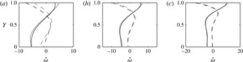
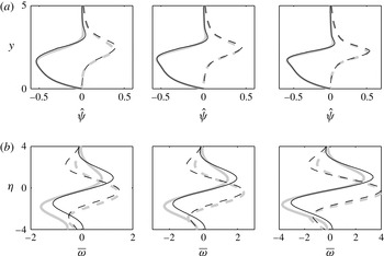
A composite solution is formed by combining the bulk (4.9) and inner (4.16) contributions and subtracting their overlap. It compares favourably to the solution to the long-wave equations (4.3) and also to the full numerical solution of (4.1) in figure 7. In particular, the matched asymptotics are able to accurately capture the amplification of the vorticity near the upper wall.
Comparison of numerics (grey line), long-wave (dark grey line) and
 ${\mathcal{W}}\gg 1$
(black line) solutions for the vorticity,
 $\hat{{\it\omega}}=-\text{d}_{Y}^{2}\hat{{\it\psi}}$
. The parameters correspond to those in figure 6 and from (a)–(c)
 ${\mathcal{W}}=\{10,20,40\}$
.

The asymptotic solution is instructive. Unlike the Hankel function solution of the long-wave equations (4.3), the matched asymptotic solution (4.9), (4.16) delineates the origin of the vorticity distribution across the channel and of the vorticity amplification at the top wall. It also demonstrates that the flow response in the shallow-elastic regime is dominated by elastic effects. The distortion of the highly tensioned mean-flow streamlines by the surface undulations establishes an irrotational polymer force field in the bulk of the channel (
 $\hat{{\it\chi}}\propto -d_{Y}^{2}\hat{{\it\Phi}}=0$
in 4.6a
), which corresponds to a constant perturbation vorticity (
 $\hat{{\it\omega}}_{0}\approx -2{\hat{h}}$
from 4.9). The perturbed, total velocity streamlines are parallel to the bottom wall topography in this layer. Close to the upper wall, the no-slip condition generates large vorticity gradients, with corresponding variations in polymer torque. The wall vorticity can be evaluated from the inner solution,
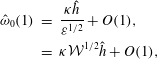 $$\begin{eqnarray}\displaystyle \hat{{\it\omega}}_{0}(1) & = & \displaystyle \frac{{\it\kappa}{\hat{h}}}{{\it\varepsilon}^{1/2}}+O(1),\nonumber\\ \displaystyle & = & \displaystyle {\it\kappa}{\mathcal{W}}^{1/2}{\hat{h}}+O(1),\end{eqnarray}$$
and has been amplified relative to its value in the bulk,
 $\hat{{\it\omega}}\approx -2{\hat{h}}$
, by a factor
 ${\it\kappa}{\mathcal{W}}^{1/2}$
. This effect is therefore increasingly important with increasing polymer concentration and elasticity
4.2 Deep-elastic flow
The terminology ‘deep elastic’ refers to flow configurations where
 ${\it\alpha}\gtrsim 1$
and
 ${\it\Sigma}\gtrsim 1$
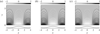
. The second of these requirements places the critical layer sufficiently far from the wall such that vorticity wave propagation dominates the dynamics of the perturbation field rather than base-flow advection. Two examples of the vorticity induced by the lower wall in this regime are reported in figure 8, alongside a Newtonian solution from the deep-viscous regime. The vorticity appears unchanged from the Newtonian solution irrespective of the choice of parameters, and
 $|\hat{{\it\omega}}|$
is monotonically decaying with height.
Vortical perturbations (top) induced by the wavy wall (bottom) in the deep-elastic regime. Filled contours are the spanwise vorticity, lines are the streamfunction. (a) Newtonian flow (deep viscous)
 ${\it\alpha}=10$
,
 $R=5$
. (b) Deep-elastic flow,
 ${\it\alpha}=10$
and
 ${\it\Sigma}=8.9$
with
 $R=5$
,
 ${\it\beta}=0.8$
,
 $W=10$
. (c) Deep-elastic flow,
 ${\it\alpha}=10$
and
 ${\it\Sigma}=34.6$
with
 $R=5$
,
 ${\it\beta}=0.5$
,
 $W=60$
.

In this section we construct an asymptotic solution to (2.7) assuming
 ${\it\Sigma}\gg 1$
, and demonstrate that the vorticity is unchanged from the Newtonian deep-viscous solution for any choice of
 $W$
or
 ${\it\beta}$
. We then examine the high-Weissenberg-number limit in order to explain why the polymer does not alter the structure of the perturbation field in deep channels with high elasticity.
We assume that
 ${\it\alpha}\gg 1$
so that the upper wall no longer appears in the problem. Then, defining the scaled polymer potential
 ${\it\Phi}\equiv {\it\varphi}/W$
, the governing system (2.7) becomes
 $$\begin{eqnarray}\text{i}k\dot{{\it\gamma}}y\left(\frac{\text{d}^{2}}{\text{d}y^{2}}-k^{2}\right){\it\psi}=\frac{{\it\Sigma}^{2}}{2}\left[\frac{{\it\beta}}{(1-{\it\beta})W}\left(\frac{\text{d}^{2}}{\text{d}y^{2}}-k^{2}\right)^{2}{\it\psi}+\left(\frac{\text{d}^{2}}{\text{d}y^{2}}-k^{2}\right){\it\Phi}\right],\end{eqnarray}$$
 $$\begin{eqnarray}\left(\text{i}k\dot{{\it\gamma}}y+\frac{1}{W}\right){\it\Phi}=\left[-2k^{2}\dot{{\it\gamma}}^{2}+\frac{2\text{i}\dot{{\it\gamma}}}{W}\frac{\text{d}}{\text{d}y}+\frac{1}{W^{2}}\left(\frac{\text{d}^{2}}{\text{d}y^{2}}-k^{2}\right)\right]{\it\psi}.\end{eqnarray}$$
 ${\it\Sigma}\gg 1$
, we seek a solution in powers of
 ${\it\varepsilon}\equiv 1/{\it\Sigma}^{2}\ll 1$
,
 $$\begin{eqnarray}\displaystyle & \displaystyle {\it\psi}(y;{\it\varepsilon})={\it\psi}_{0}(y)+{\it\varepsilon}{\it\psi}_{1}(y)+\cdots , & \displaystyle\end{eqnarray}$$
 $$\begin{eqnarray}\displaystyle & \displaystyle {\it\Phi}(y;{\it\varepsilon})={\it\Phi}_{0}(y)+{\it\varepsilon}{\it\Phi}_{1}(y)+\cdots , & \displaystyle\end{eqnarray}$$
 $$\begin{eqnarray}\displaystyle & \displaystyle 0=\frac{{\it\beta}}{W}\left(\frac{\text{d}^{2}}{\text{d}y^{2}}-k^{2}\right)^{2}{\it\psi}_{0}+(1-{\it\beta})\left(\frac{\text{d}^{2}}{\text{d}y^{2}}-k^{2}\right){\it\Phi}_{0}, & \displaystyle\end{eqnarray}$$
 $$\begin{eqnarray}\displaystyle & \displaystyle \left(\text{i}k\dot{{\it\gamma}}y+\frac{1}{W}\right){\it\Phi}_{0}=\left[-2k^{2}\dot{{\it\gamma}}^{2}+\frac{2\text{i}\dot{{\it\gamma}}}{W}\frac{\text{d}}{\text{d}y}+\frac{1}{W^{2}}\left(\frac{\text{d}^{2}}{\text{d}y^{2}}-k^{2}\right)\right]{\it\psi}_{0}. & \displaystyle\end{eqnarray}$$
 $$\begin{eqnarray}\displaystyle {\it\psi}_{0}(y) & = & \displaystyle E_{0}y\text{e}^{-ky}+F_{0}y\text{e}^{ky}\nonumber\\ \displaystyle & & \displaystyle +\,G_{0}\text{e}^{-ky}{\mathcal{U}}\left(\frac{(1-{\it\beta})(1-\text{i}\dot{{\it\gamma}}W)}{{\it\beta}},\frac{2(1-{\it\beta})}{{\it\beta}},2\left(ky+\frac{1}{\text{i}\dot{{\it\gamma}}W{\it\beta}}\right)\right)\nonumber\\ \displaystyle & & \displaystyle +\,H_{0}\text{e}^{-ky}{\mathcal{M}}\left(\frac{(1-{\it\beta})(1-\text{i}\dot{{\it\gamma}}W)}{{\it\beta}},\frac{2(1-{\it\beta})}{{\it\beta}},2\left(ky+\frac{1}{\text{i}\dot{{\it\gamma}}W{\it\beta}}\right)\right),\end{eqnarray}$$
where
 ${\mathcal{U}}$
and
 ${\mathcal{M}}$
are Kummer’s functions (Abramowitz & Stegun Reference Abramowitz and Stegun1964). After discarding exponentially growing terms and applying the boundary conditions at the lower wall, we obtain
 ${\it\psi}_{0}(y)=-h\dot{{\it\gamma}}y\text{e}^{-ky}$
, which is identical to the leading-order Newtonian solution in the deep-viscous regime reported by Charru & Hinch (Reference Charru and Hinch2000). The polymer does not have an effect on the flow field to leading order for any value of
 $W$
provided
 ${\it\Sigma}\gg 1$
.
The above result is simple to understand in the limit of fast polymer relaxation,
 $W\ll 1$
. As noted in § 3.1, in this limit the polymer behaves like additional solvent,
 ${\it\Phi}_{0}\sim (1/2W)(\text{d}_{y}^{2}-k^{2}){\it\psi}_{0}$
. The flow is therefore dominated by vorticity diffusion, and the streamfunction satisfies the biharmonic equation
 $(\text{d}_{y}^{2}-k^{2})^{2}{\it\psi}_{0}=0$
.
Some additional explanation is required in the high-Weissenberg-number limit, where it is not obvious why the flow response should appear unaffected by the large base-state stress. If
 $W\gg 1$
, we may approximate (4.21) by
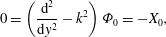 $$\begin{eqnarray}\displaystyle & \displaystyle 0=\left(\frac{\text{d}^{2}}{\text{d}y^{2}}-k^{2}\right){\it\Phi}_{0}=-X_{0}, & \displaystyle\end{eqnarray}$$
 $$\begin{eqnarray}\displaystyle & \displaystyle \text{i}k\dot{{\it\gamma}}y{\it\Phi}_{0}=-2k^{2}\dot{{\it\gamma}}^{2}{\it\psi}_{0}, & \displaystyle\end{eqnarray}$$
 $X_{0}={\it\chi}_{0}/W$
is the scaled polymer torque. The dominant balance is analogous to the large-
 ${\mathcal{W}}$
limit of the long-wave equations (4.6). According to (4.23b
), polymer forces are generated by displacement of the highly tensioned mean-flow streamlines, similar to the flow in the shallow-elastic regime. However, without the influence of the upper wall, there is no reason for a rapid flow adjustment and the Orr–Sommerfeld equation (4.23a
) indicates that the irrotational polymer force field decays exponentially in
 $y$
. This results in a perturbation flow which has the same form as the Newtonian deep-viscous regime.
4.3 Transcritical flow
The terminology ‘transcritical’ is associated with flows where
 ${\it\alpha}>{\it\Sigma}$
and
 ${\it\Sigma}\lesssim 1$
. These criteria correspond to the existence of a critical layer inside the flow domain and whose height,
 $y={\it\Sigma}$
or
 $y^{\ast }=\sqrt{2{\it\nu}_{p}{\it\varsigma}}$
, is within one wavelength from the lower wall. Across this critical layer, the base-flow velocity changes from subcritical to supercritical relative to the vorticity longitudinal wave speed. It is the same surface across which Yoo & Joseph (Reference Yoo and Joseph1985) find a change in type in the equations for an upper convected Maxwell fluid. Here, the focus is the mechanism for vorticity amplification at this layer.
Vortical perturbations (top) induced by the wavy wall (bottom) in transcritical flows with constant
 ${\it\alpha}=10$
and
 ${\it\Sigma}=2.45$
. Filled contours are the spanwise vorticity, lines are the streamfunction. The polymer viscosity is fixed at
 ${\it\beta}=0.5$
and the bulk Reynolds and Weissenberg numbers are varied: (a)
 $R=250$
,
 $W=15$
; (b)
 $R=500$
,
 $W=30$
; (c)
 $R=1000$
,
 $W=60$
.

Vortical perturbations (top) induced by the wavy wall (bottom) in transcritical flows with constant vorticity wave speed,
 $\sqrt{2W(1-{\it\beta})/R}=0.24$
(
 $R=500$
,
 $W=30$
,
 ${\it\beta}=0.5$
), with varying
 ${\it\alpha}$
. Filled contours are the spanwise vorticity, lines are the streamfunction. (a)
 ${\it\alpha}=5$
; (b)
 ${\it\alpha}=10$
; (c)
 ${\it\alpha}=15$
.

The spanwise-vorticity perturbation and associated streamfunction that are induced by the wavy wall are reported in figure 9 for three transcritical conditions. The critical layer height,
 ${\it\Sigma}$
, is held constant, and the bulk Reynolds and Weissenberg numbers are varied. In each case the spanwise vorticity is amplified around
 $y={\it\Sigma}$
. The
 ${\it\omega}$
-perturbation field close to
 $y={\it\Sigma}$
is arranged in stripes of positive and negative vorticity which are tilted forward with the shear and which become progressively stronger as
 $R$
and
 $W$
are increased.
In figure 10,
 ${\it\alpha}$
is varied while the bulk flow parameters are held fixed, which corresponds to a fixed vorticity wave speed. As a result, the dimensional
 $y^{\ast }$
-location of the critical layer is unchanged. However, relative to the roughness length scale, the critical layer height,
 $y={\it\Sigma}$
, increases with
 ${\it\alpha}$
and figure 10 captures the transition between the transcritical and deep-elastic regimes. As
 ${\it\Sigma}$
increases, the vorticity decays with height in
 $y\lesssim {\it\Sigma}$
and amplification at
 $y={\it\Sigma}$
is much less effective.
In order to examine the vorticity generation at the critical layer, the high-Weissenberg-number limit of the governing equations (2.7) will be derived. In this limit only the effects of the kinematic torque amplification mechanism and streamwise normal stress remain in the polymer-torque equation. The kinematic amplification is interpreted in terms of the polymer forces, before the equations for
 ${\it\omega}$
and
 ${\it\chi}$
are combined to form an ‘elastic-Rayleigh’ equation for the spanwise vorticity. In this equation the torque kinematics appear as a forcing term, and the efficacy of this term to generate vorticity is shown to depend on the relative values of two frequencies: the frequency at which the lower wall appears to oscillate relative to an observer moving with the shear and the frequency of a streamwise-travelling elastic vorticity wave with wavenumber
 $k$
. We demonstrate that there is a resonance between these two frequencies at the critical layer, before developing an approximate solution for the perturbation streamfunction using matched asymptotic expansions. The solution provides explicit expressions for the critical layer thickness and the level of vorticity amplification due to the resonance at
 $y={\it\Sigma}$
.
The vorticity amplification in the transcritical regime is increasingly pronounced at large Weissenberg numbers. Therefore, the small parameter,
 ${\it\varepsilon}\equiv 1/W\ll 1$
, is defined and an asymptotic expansion is adopted,
 $$\begin{eqnarray}\displaystyle & \displaystyle {\it\psi}(y;{\it\varepsilon})={\it\psi}_{0}(y)+{\it\varepsilon}{\it\psi}_{1}(y)+\cdots , & \displaystyle\end{eqnarray}$$
 $$\begin{eqnarray}\displaystyle & \displaystyle {\it\Phi}(y;{\it\varepsilon})={\it\Phi}_{0}(y)+{\it\varepsilon}{\it\Phi}_{1}(y)+\cdots , & \displaystyle\end{eqnarray}$$
 ${\it\Phi}={\it\varepsilon}{\it\varphi}$
is the scaled polymer potential. The leading-order approximation of (2.7) is
 $$\begin{eqnarray}\text{i}k\dot{{\it\gamma}}y\left(\frac{\text{d}^{2}}{\text{d}y^{2}}-k^{2}\right){\it\psi}_{0}=\frac{{\it\Sigma}^{2}}{2}\left(\frac{\text{d}^{2}}{\text{d}y^{2}}-k^{2}\right){\it\Phi}_{0},\end{eqnarray}$$
and
 $$\begin{eqnarray}\text{i}k\dot{{\it\gamma}}y{\it\Phi}_{0}=-2k^{2}\dot{{\it\gamma}}^{2}{\it\psi}_{0}.\end{eqnarray}$$
Again, the high-Weissenberg-number limit means that polymer forces are primarily generated by an induced curvature in the tensioned mean-flow streamlines. In this particular regime, it is instructive to write (4.25) in terms of the vorticity,
 ${\it\omega}$
, and polymer torque,
 ${\it\chi}$
(cf. equation (2.9)),
 $$\begin{eqnarray}\displaystyle & \displaystyle \text{i}k\dot{{\it\gamma}}y{\it\omega}_{0}=\frac{{\it\Sigma}^{2}}{2}X_{0}, & \displaystyle\end{eqnarray}$$
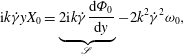 $$\begin{eqnarray}\displaystyle & \displaystyle \text{i}k\dot{{\it\gamma}}yX_{0}=\underbrace{2\text{i}k\dot{{\it\gamma}}\frac{\text{d}{\it\Phi}_{0}}{\text{d}y}}_{\mathscr{S}}-2k^{2}\dot{{\it\gamma}}^{2}{\it\omega}_{0}, & \displaystyle\end{eqnarray}$$
 $X\equiv {\it\varepsilon}{\it\chi}=-(\text{d}_{y}^{2}-k^{2}){\it\Phi}$
. The term labelled
 $\mathscr{S}$
corresponds to the kinematic mechanism for polymer-torque amplification,
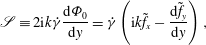 $$\begin{eqnarray}\mathscr{S}\equiv 2\text{i}k\dot{{\it\gamma}}\frac{\text{d}{\it\Phi}_{0}}{\text{d}y}=\dot{{\it\gamma}}\left(\text{i}k\tilde{f}_{x}-\frac{\text{d}\tilde{f}_{y}}{\text{d}y}\right),\end{eqnarray}$$
and
 $\tilde{f}_{i}\equiv {\it\varepsilon}f_{i}$
are the scaled polymer forces. The relative realignment of streamwise layers of varying polymer force by the mean shear generates a perturbation torque at a point.
Combining (4.26) into a single equation yields
 $$\begin{eqnarray}({\it\varpi}^{2}(y)-k^{2}c_{{\it\omega}}^{2}){\it\omega}_{0}=-\text{i}kc_{{\it\omega}}{\it\Sigma}\frac{\text{d}{\it\Phi}_{0}}{\text{d}y},\end{eqnarray}$$
where
 ${\it\varpi}(y)\equiv k\dot{{\it\gamma}}y$
is the apparent frequency at which the vorticity source (lower wall) appears to oscillate relative to an observer travelling with the mean flow at a height
 $y$
, while
 $c_{{\it\omega}}\equiv \dot{{\it\gamma}}{\it\Sigma}$
is the dimensionless speed of a streamwise-travelling vorticity wave in the viscoelastic flow. The kinematic torque amplification appears as a forcing term on the right-hand side. Equation (4.28) is known as the elastic-Rayleigh equation (Azaiez & Homsy Reference Azaiez and Homsy1994; Rallison & Hinch Reference Rallison and Hinch1995; Ray & Zaki Reference Ray and Zaki2014, Reference Ray and Zaki2015).
In equation (4.28),
 $kc_{{\it\omega}}$
represents the frequency of an elastic vorticity with wavenumber
 $k$
and appears as the natural frequency. At the critical layer,
 $y={\it\Sigma}$
, a travelling observer sees the wall as a vorticity source sweeping by at the elastic wave speed. Or, equivalently, the critical layer is the height where a travelling observer sees perturbations oscillating with a frequency that matches the frequency of an elastic wave of the same wavelength. The resulting resonance at the particular location in the flow corresponds to a singular point in the elastic-Rayleigh equation, and the torque amplification mechanism becomes most effective.
While equation (4.28) identifies the mechanism for vorticity amplification around
 $y={\it\Sigma}$
, the thickness of the critical layer is unknown. Furthermore, the level of vorticity amplification at the critical layer cannot be deduced from (4.28), in which
 $y={\it\Sigma}$
is a singular point. In order to address these issues, a solution to the viscoelastic Orr–Sommerfeld system (2.7) is now constructed using matched asymptotic expansions with
 ${\it\varepsilon}\equiv 1/W\ll 1$
as the small parameter.
Bulk solution: the leading term in an expansion in powers of
 ${\it\varepsilon}$
satisfies the elastic-Rayleigh equation derived above (4.28), which determines the perturbation field in the bulk of the channel. In terms of the streamfunction,
 ${\it\psi}_{0}$
, this equation is,
 $$\begin{eqnarray}\frac{\text{d}^{2}}{\text{d}y^{2}}\left(\frac{{\it\psi}_{0}}{y}\right)+\frac{2y}{(y^{2}-{\it\Sigma}^{2})}\frac{\text{d}}{\text{d}y}\left(\frac{{\it\psi}_{0}}{y}\right)-k^{2}\left(\frac{{\it\psi}_{0}}{y}\right)=0.\end{eqnarray}$$
Equation (4.29) has regular singular points at
 $y={\it\Sigma}$
and
 $y=-{\it\Sigma}$
, the second of which lies outside of the flow domain. The solution may therefore be sought as a Frobenius series around
 $y={\it\Sigma}$
(Bender & Orszag Reference Bender and Orszag1978). Above the critical layer,
 $y>{\it\Sigma}$
, the expression for
 ${\it\psi}_{0}(y)$
is
 $$\begin{eqnarray}{\it\psi}_{0}^{+}(y)=A_{0}^{+}y\mathop{\sum }_{j=0}^{\infty }b_{j}\left(y-{\it\Sigma}\right)^{j}+B_{0}^{+}y\left(\mathop{\sum }_{j=1}^{\infty }c_{j}\left(y-{\it\Sigma}\right)^{j}+\mathop{\sum }_{j=0}^{\infty }b_{j}(y-{\it\Sigma})^{j}\,\text{log}|y-{\it\Sigma}|\right).\end{eqnarray}$$
The series coefficients,
 $b_{j}$
and
 $c_{j}$
, are provided in appendix A. Below the critical layer the streamfunction is written
 $$\begin{eqnarray}{\it\psi}_{0}^{-}(y)=A_{0}^{-}y\mathop{\sum }_{j=0}^{\infty }b_{j}(y-{\it\Sigma})^{j}+B_{0}^{-}y\left(\mathop{\sum }_{j=1}^{\infty }c_{j}(y-{\it\Sigma})^{j}+\mathop{\sum }_{j=0}^{\infty }b_{j}(y-{\it\Sigma})^{j}(\text{log}|y-{\it\Sigma}|-\text{i}{\rm\pi})\!\right),\end{eqnarray}$$
where the branch chosen for the logarithm is not arbitrary, but is motivated by the solution in the critical layer which is constructed below. Note that the series (4.30) have a radius of convergence which extends only as far as the next singular point of the elastic-Rayleigh equation (4.29), which is at
 $y=-{\it\Sigma}$
. Therefore, the expression for
 ${\it\psi}_{0}^{+}(y)$
(4.30a
) only converges below
 $y=3{\it\Sigma}$
. However, the present focus is the behaviour around the critical layer,
 $y={\it\Sigma}$
, and we do not attempt to patch this series to an expression valid for large
 $y$
.
Critical layer: the kinematic amplification mechanism is most effective at the critical layer. At this location a resonance occurs between the oscillation frequency of the wall vorticity, as measured by an observer travelling with the base flow, and the frequency of an elastic wave with wavenumber
 $k$
. This behaviour corresponds to a singular point in the elastic-Rayleigh equation (4.29) and motivates an examination of the Orr–Sommerfeld system (2.7) in the vicinity of the critical layer. We assume an internal boundary layer at
 $y={\it\Sigma}$
of thickness
 ${\it\delta}_{c}({\it\varepsilon})$
and adopt the rescaling
 ${\it\eta}\equiv (y-{\it\Sigma})/{\it\delta}_{c}({\it\varepsilon})$
. In terms of
 ${\it\eta}$
the bulk Frobenius solutions (4.30),
 $$\begin{eqnarray}\displaystyle & \displaystyle {\it\psi}_{0}^{+}({\it\eta})\sim A_{0}^{+}{\it\Sigma}+B_{0}^{+}{\it\Sigma}(\text{log}|{\it\eta}|+\text{log}{\it\delta}_{c})+\cdots , & \displaystyle\end{eqnarray}$$
 $$\begin{eqnarray}\displaystyle & \displaystyle {\it\psi}_{0}^{-}({\it\eta})\sim A_{0}^{-}{\it\Sigma}+B_{0}^{-}{\it\Sigma}(\text{log}|{\it\eta}|-\text{i}{\rm\pi}+\text{log}{\it\delta}_{c})+\cdots , & \displaystyle\end{eqnarray}$$
 $$\begin{eqnarray}\overline{{\it\psi}}({\it\eta})=\log {\it\delta}_{c}\overline{{\it\psi}}_{-1}({\it\eta})+\overline{{\it\psi}}_{0}({\it\eta})+\cdots ,\end{eqnarray}$$
where
 $\overline{{\it\psi}}({\it\eta})={\it\psi}(y)$
is the streamfunction expressed in terms of the critical layer coordinate and the term appearing at
 $O(\log {\it\delta}_{c})$
is an eigensolution required for matching.
In terms of the stretched coordinate,
 ${\it\eta}$
, the full Orr–Sommerfeld system (2.7) becomes,
 $$\begin{eqnarray}\displaystyle & \hspace{-16.99998pt}\displaystyle \text{i}k\dot{{\it\gamma}}({\it\Sigma}+{\it\delta}_{c}{\it\eta})\!\left(\frac{1}{{\it\delta}_{c}^{2}}\frac{\text{d}^{2}}{\text{d}{\it\eta}^{2}}-k^{2}\right)\overline{{\it\psi}}=\frac{{\it\Sigma}^{2}}{2}\!\left[\frac{{\it\beta}{\it\varepsilon}}{(1-{\it\beta})}\!\left(\frac{1}{{\it\delta}_{c}^{2}}\frac{\text{d}^{2}}{\text{d}{\it\eta}^{2}}-k^{2}\right)^{2}\!\overline{{\it\psi}}+\!\left(\frac{1}{{\it\delta}_{c}^{2}}\frac{\text{d}^{2}}{\text{d}{\it\eta}^{2}}-k^{2}\!\right)\overline{{\it\Phi}}\right]\!,\hspace{-20.00003pt} & \displaystyle \nonumber\\ \displaystyle & & \displaystyle\end{eqnarray}$$
 $$\begin{eqnarray}\displaystyle & \hspace{-18.00005pt}\displaystyle \text{i}k\dot{{\it\gamma}}({\it\Sigma}+{\it\delta}_{c}{\it\eta})\overline{{\it\Phi}}+{\it\varepsilon}\overline{{\it\Phi}}=\bigg[-\!2k^{2}\dot{{\it\gamma}}^{2}+2\text{i}k\dot{{\it\gamma}}\frac{{\it\varepsilon}}{{\it\delta}_{c}}\frac{\text{d}}{\text{d}{\it\eta}}+{\it\varepsilon}^{2}\left(\frac{1}{{\it\delta}_{c}^{2}}\frac{\text{d}^{2}}{\text{d}{\it\eta}^{2}}-k^{2}\right)\bigg]\overline{{\it\psi}},\hspace{-10.00002pt} & \displaystyle\end{eqnarray}$$
 $\overline{{\it\Phi}}({\it\eta})={\it\Phi}(y)$
is the scaled polymer potential. If
 ${\it\delta}_{c}>{\it\varepsilon}$
, then according to (4.33b
) the polymer potential
 $\overline{{\it\Phi}}$
is dominated by the effects of the normal stress,
 $T_{11}$
, similar to the bulk flow (4.30). This balance implies that
 $\text{i}k\dot{{\it\gamma}}({\it\Sigma}+{\it\delta}_{c}{\it\eta})\overline{{\it\Phi}}\approx -2k^{2}\dot{{\it\gamma}}^{2}\overline{{\it\psi}}$
, which is substituted into (4.33a
) and yields,
 $$\begin{eqnarray}\displaystyle & & \displaystyle \text{i}k\dot{{\it\gamma}}({\it\Sigma}+{\it\delta}_{c}{\it\eta})\left(\frac{1}{{\it\delta}_{c}^{2}}\frac{\text{d}^{2}}{\text{d}{\it\eta}^{2}}-k^{2}\right)\overline{{\it\psi}}\nonumber\\ \displaystyle & & \displaystyle \quad \approx \frac{{\it\Sigma}^{2}}{2}\bigg[\frac{{\it\beta}{\it\varepsilon}}{(1-{\it\beta})}\left(\frac{1}{{\it\delta}_{c}^{2}}\frac{\text{d}^{2}}{\text{d}{\it\eta}^{2}}-k^{2}\right)^{2}\overline{{\it\psi}}+\underbrace{\frac{2\text{i}k\dot{{\it\gamma}}}{{\it\Sigma}}\left(\frac{1}{{\it\delta}_{c}^{2}}\frac{\text{d}^{2}}{\text{d}{\it\eta}^{2}}-k^{2}\right)\left(\overline{{\it\psi}}-\frac{{\it\delta}_{c}{\it\eta}}{{\it\Sigma}}\overline{{\it\psi}}+\cdots \,\right)}_{\overline{{\it\Phi}}}\bigg],\qquad \hspace{-20.00003pt}\nonumber\\ \displaystyle & & \displaystyle\end{eqnarray}$$
As anticipated, the leading term in
 $\overline{{\it\Phi}}$
on the right-hand side cancels with the leading advection term on the left-hand side. The dominant balance between advection, diffusion in the solvent and polymer potential due to
 $T_{11}$
then suggests a critical layer thickness
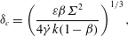 $$\begin{eqnarray}{\it\delta}_{c}=\left(\frac{{\it\varepsilon}{\it\beta}{\it\Sigma}^{2}}{4\dot{{\it\gamma}}k(1-{\it\beta})}\right)^{1/3},\end{eqnarray}$$
where the factor of
 $4$
is introduced for convenience. In dimensional variables
 ${\it\delta}_{c}^{\ast }=({\it\nu}_{s}/2\dot{{\it\gamma}}^{\ast }k^{\ast })^{1/3}$
, which is a diffusion length in the solvent. The scaling is also consistent with the original assumption regarding the relative importance of the base-state stresses in the critical layer:
 $T_{12}$
appears at
 $O({\it\varepsilon}^{2/3})$
in (4.33b
).
The dominant balance between advection, polymer torque generated by
 $T_{11}$
and solvent diffusion in (4.34) leads to
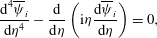 $$\begin{eqnarray}\frac{\text{d}^{4}\overline{{\it\psi}}_{i}}{\text{d}{\it\eta}^{4}}-\frac{\text{d}}{\text{d}{\it\eta}}\left(\text{i}{\it\eta}\frac{\text{d}\overline{{\it\psi}}_{i}}{\text{d}{\it\eta}}\right)=0,\end{eqnarray}$$
which is satisfied by the two leading terms in the inner expansion (4.32). Equation (4.36) can be written as an inhomogeneous Airy equation for the derivative
 $\text{d}_{{\it\eta}}\overline{{\it\psi}}_{0}$
, although it is more convenient to express the solutions in integral form,
 $$\begin{eqnarray}\displaystyle \overline{{\it\psi}}_{i}({\it\eta}) & = & \displaystyle \overline{A}_{i}+\overline{B}_{i}\int _{{\it\sigma}}^{\infty }\left(\frac{1}{s}\right)\text{exp}\left(-\frac{s^{3}}{3}-\text{i}s{\it\eta}\right)\text{d}s\nonumber\\ \displaystyle & & \displaystyle +\,\overline{C}_{i}\int _{{\it\sigma}}^{\infty }\left(\frac{1}{s}\right)\text{exp}\left(-\frac{s^{3}}{3}+\frac{s{\it\eta}(\sqrt{3}+\text{i})}{2}\right)\text{d}s\nonumber\\ \displaystyle & & \displaystyle +\,\overline{D}_{i}\int _{{\it\sigma}}^{\infty }\left(\frac{1}{s}\right)\text{exp}\left(-\frac{s^{3}}{3}+\frac{s{\it\eta}(-\sqrt{3}+\text{i})}{2}\right)\text{d}s,\end{eqnarray}$$
where the limit
 ${\it\sigma}\rightarrow 0$
should be taken and the constant
 $\overline{A}_{i}$
contains terms which eliminate the logarithmic divergence associated with this limit (see appendix A). This statement is made explicit below, where
 $\overline{{\it\psi}}({\it\eta})$
is matched to the elastic-Rayleigh solutions in the bulk.
Assuming that the critical layer and the wall are well separated,
 ${\it\Sigma}\gg {\it\delta}_{c}$
, solutions which are exponentially growing as
 ${\it\eta}\rightarrow \pm \infty$
must be discarded. The critical layer streamfunction thus takes the form,
 $$\begin{eqnarray}\overline{{\it\psi}}_{i}({\it\eta})=\overline{A}_{i}+\overline{B}_{i}\int _{{\it\sigma}}^{\infty }\left(\frac{1}{s}\right)\text{exp}\left(-\frac{s^{3}}{3}-\text{i}s{\it\eta}\right)\text{d}s.\end{eqnarray}$$
In appendix A the method of steepest descents is applied to the integral appearing in (4.38) to obtain the behaviour of the inner streamfunction as
 ${\it\eta}\rightarrow \pm \infty$
,
 $$\begin{eqnarray}\displaystyle & \displaystyle \overline{{\it\psi}}_{i}({\it\eta}\rightarrow \infty )\sim \overline{A}_{i}+\overline{B}_{i}\left(-{\it\gamma}-\frac{\text{i}{\rm\pi}}{2}-\log {\it\sigma}-\text{log}|{\it\eta}|\right), & \displaystyle\end{eqnarray}$$
 $$\begin{eqnarray}\displaystyle & \displaystyle \overline{{\it\psi}}_{i}({\it\eta}\rightarrow -\infty )\sim \overline{A}_{i}+\overline{B}_{i}\left(-{\it\gamma}+\frac{\text{i}{\rm\pi}}{2}-\log {\it\sigma}-\text{log}|{\it\eta}|\right), & \displaystyle\end{eqnarray}$$
 ${\it\gamma}=0.5772\ldots \,$
is the Euler–Mascheroni constant and there is a phase change of
 ${\rm\pi}$
across the critical layer. Matching these expressions to the bulk streamfunction near
 $y={\it\Sigma}$
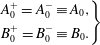
(4.31) reduces the number of unknown constants in the system to two. Across the critical layer, the constants in the expressions for the bulk streamfunction (4.30) are unchanged,
 $$\begin{eqnarray}\displaystyle \left.\begin{array}{@{}c@{}}\displaystyle A_{0}^{+}=A_{0}^{-}\equiv A_{0},\\ \displaystyle B_{0}^{+}=B_{0}^{-}\equiv B_{0}.\end{array}\right\} & & \displaystyle\end{eqnarray}$$
The constants appearing in the critical layer solution are,
 $$\begin{eqnarray}\displaystyle \left.\begin{array}{@{}c@{}}\overline{A}_{-1}={\it\Sigma}B_{0},\quad \overline{B}_{-1}=0;\\ \overline{A}_{0}={\it\Sigma}A_{0}+{\it\Sigma}B_{0}\left(-{\it\gamma}-{\displaystyle \frac{\text{i}{\rm\pi}}{2}}-\log {\it\sigma}\right),\quad \overline{B}_{0}=-{\it\Sigma}B_{0}.\end{array}\right\} & & \displaystyle\end{eqnarray}$$
The
 $O(\log {\it\delta}_{c})$
term in the critical layer is therefore a constant, and the inner streamfunction is
 $$\begin{eqnarray}\overline{{\it\psi}}({\it\eta})={\it\Sigma}B_{0}\log {\it\delta}_{c}+{\it\Sigma}A_{0}+{\it\Sigma}B_{0}\!\left(\!-{\it\gamma}-\frac{\text{i}{\rm\pi}}{2}-\log {\it\sigma}\!\right)-{\it\Sigma}B_{0}\!\int _{{\it\sigma}}^{\infty }\!\!\left(\!\frac{1}{s}\!\right)\text{exp}\left(\!-\frac{s^{3}}{3}-\text{i}s{\it\eta}\!\right)\text{d}s.\end{eqnarray}$$
In the limit
 ${\it\sigma}\rightarrow 0$
the term
 $-{\it\Sigma}B_{0}\log {\it\sigma}$
eliminates the logarithmic divergence associated with the lower limit of the integral.
The solutions to the elastic-Rayleigh equation (4.30) automatically satisfy the no penetration condition at the lower wall,
 ${\it\psi}_{0}^{-}(y=0)=0$
. One of the two remaining constants,
 $A_{0}$
and
 $B_{0}$
, can be eliminated by applying the slip condition on the streamwise perturbation velocity,
 $\text{d}_{y}{\it\psi}_{0}^{-}(y=0)=-\dot{{\it\gamma}}h$
. In deep channels,
 ${\it\alpha}\gg 1$
, the final constant would be chosen to enforce boundedness of the streamfunction far above the critical layer. In the present formulation, the series solutions to the elastic-Rayleigh equation only converge below
 $y=3{\it\Sigma}$
, and so this condition cannot be enforced without patching
 ${\it\psi}_{0}^{+}(y)$
to solutions valid for large
 $y$
. However, our focus is the vorticity amplification at the critical layer, while above
 $y\approx {\it\Sigma}$
the perturbation decays. Therefore, we instead impose the artificial condition
 ${\it\psi}_{0}^{+}(y=8{\it\Sigma}/3)=0$
in order to determine the final unknown constant. In domains where
 ${\it\alpha}<3{\it\Sigma}$
, we may enforce the no-penetration condition at the top wall,
 ${\it\psi}_{0}^{+}(y={\it\alpha})=0$
. This approach introduces a small slip velocity, which could be eliminated by examining the perturbations in a thin solvent boundary layer at
 $y={\it\alpha}$
, similar to the approach taken in the shallow-elastic regime (see § 4.1).
Comparison of numerical (grey) and asymptotic (black) solutions in the transcritical regime. (a) Composite streamfunction formed from solutions to the elastic-Rayleigh (4.30) and critical layer (4.42) equations. (b) Critical layer vorticity,
 $\overline{{\it\omega}}$
. From left to right:
 ${\it\alpha}=10$
,
 ${\it\Sigma}=2.5$
, with
 $R=500$
,
 $W=30$
,
 ${\it\beta}=0.5$
;
 ${\it\alpha}=10$
,
 ${\it\Sigma}=2.5$
, with
 $R=1000$
,
 $W=60$
,
 ${\it\beta}=0.5$
;
 ${\it\alpha}=10$
,
 ${\it\Sigma}=2.24$
, with
 $R=2000$
,
 $W=100$
,
 ${\it\beta}=0.5$
.

A composite asymptotic solution is formed by combining the bulk (4.30) and inner (4.42) solutions and subtracting their overlapping values. It is compared to numerical solutions for three parameter sets in the transcritical regime in figure 11(a). The asymptotic solution compares favourably with the numerics, and becomes increasingly accurate as the Weissenberg number is increased.
The critical layer vorticity computed from the inner solution (4.42) is also compared to the numerical solution in figure 11(b), with increasingly good agreement at higher
 $W$
. Furthermore, the vorticity at the critical layer may be estimated explicitly,
 $$\begin{eqnarray}\displaystyle {\it\omega}_{0}(y={\it\Sigma}) & = & \displaystyle -\frac{{\it\Sigma}B_{0}}{{\it\delta}_{c}^{2}}\int _{0}^{\infty }s\;\text{exp}\left(-\frac{s^{3}}{3}\right)\text{d}s,\nonumber\\ \displaystyle & = & \displaystyle -\frac{{\it\Sigma}B_{0}3^{-1/3}}{{\it\delta}_{c}^{2}}{\it\Gamma}\left(\frac{2}{3}\right)\approx -\frac{0.9389{\it\Sigma}B_{0}}{{\it\delta}_{c}^{2}}.\end{eqnarray}$$
Numerical calculations of
 $B_{0}$
over a range of
 ${\it\Sigma}$
(not shown) demonstrate a dependence
 $B_{0}\propto \sqrt{{\it\Sigma}}\text{exp}(-{\it\Sigma})$
and so the vorticity
 ${\it\omega}_{0}\propto {\it\Sigma}^{3/2}\text{exp}(-{\it\Sigma})/{\it\delta}_{c}^{2}$
. The exponential decay with
 ${\it\Sigma}$
reflects the weakened propensity for vorticity amplification as the critical layer is moved farther from the wall due to decay in
 $y<{\it\Sigma}$
, as was remarked in connection with figure 10. The dependence on the solvent diffusion length is intuitive: increasingly sharp gradients are generated across thinner critical layers.
The transcritical regime,
 ${\it\alpha}>{\it\Sigma}$
and
 ${\it\Sigma}\lesssim 1$
, is perhaps the most intriguing in the phase diagram because the maximum vorticity is observed in the bulk of the fluid, away from the bottom topography. This non-local vorticity amplification was explained using the elastic-Rayleigh equation which shows that when curvature acts onto the base-state
 $T_{11}$
stresses, it generates polymer torque. This torque then acts as forcing on the right-hand side of the vorticity equation, and its effectiveness at generating vorticity depends on the difference between two frequencies: (i) the frequency of oscillation of the vorticity source, or the undulating wall, relative to an observer travelling with the mean flow; (ii) the frequency of a streamwise-travelling elastic vorticity wave with wavenumber
 $k$
, which is a property of the viscoelastic flow configuration. When the two frequencies match, resonance occurs at the critical layer
 $y={\it\Sigma}$
, and the kinematic mechanism becomes most effective at generating vorticity. The critical layer thickness scales with the solvent diffusion,
 ${\it\delta}_{c}^{\ast }\sim ({\it\nu}_{s}/{\it\gamma}^{\ast }k^{\ast })^{1/3}$
and the vorticity in this layer can be estimated by
 ${\it\omega}=O({\it\Sigma}^{3/2}\text{exp}(-{\it\Sigma})/{\it\delta}_{c}^{2})$
.
5 Localized roughness
The detailed analysis of the three regimes of vorticity generation above a harmonic wall topography provides the foundation for examining the flow response to general, small-amplitude surface topography. In this section the flow response to localised wall roughness is examined numerically. The phenomenology observed in these computations are then interpreted based on the analyses in § 4.
5.1 Gaussian wall bump
By exploiting the linearity of the problem, we herein extend our earlier analyses to more realistic, localized surface topographies using Fourier synthesis. We consider the flow response to a Gaussian wall bump,
 $$\begin{eqnarray}\mathscr{H}^{\ast }(x)=h^{\ast }\text{e}^{-|x^{\ast }|^{2}/l_{x}^{\ast 2}},\end{eqnarray}$$
where
 $l_{x}^{\ast }$
is now used as the reference length. The corresponding non-dimensional wall disturbance is
 $\mathscr{H}^{\prime }(x)=h\text{e}^{-|x|^{2}/l_{x}^{2}}$
, where
 $l_{x}=1$
is retained for clarity. The Fourier transform of this wall bump is also Gaussian
 $$\begin{eqnarray}\mathscr{H}(k)=\int _{-\infty }^{\infty }\mathscr{H}^{\prime }(x)\text{e}^{-\text{i}kx}\,\text{d}x=hl_{x}\sqrt{{\rm\pi}}\,\text{e}^{-l_{x}^{2}k^{2}/4},\end{eqnarray}$$
and we adopt the normalization
 $h=1$
. Note that the zeroth wavenumber,
 $k=0$
, corresponds to a mean-flow correction and is omitted from the energy and enstrophy spectra presented in this section.
While the spectral make-up of the wall disturbance (5.1b
) includes waves for which the channel will appear shallow (
 $k\rightarrow 0$
) and infinitely deep (
 $k\rightarrow \infty$
), it is helpful to introduce the parameters,
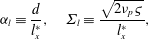 $$\begin{eqnarray}{\it\alpha}_{l}\equiv \frac{d}{l_{x}^{\ast }},\quad {\it\Sigma}_{l}\equiv \frac{\sqrt{2{\it\nu}_{p}{\it\varsigma}}}{l_{x}^{\ast }},\end{eqnarray}$$
in order to relate the present results to the earlier discussion of the wavy wall. These parameters are the normalized channel depth and ratio of the critical layer depth to the bump length scale, respectively.
Vortical perturbations (top) induced by Gaussian wall bump (bottom) in shallow flow with
 ${\it\alpha}_{l}=0.5$
. Filled contours are the spanwise vorticity, lines are the streamfunction. (a) Newtonian flow with
 $R=1$
. (b) Viscoelastic flow with
 ${\it\Sigma}_{l}=3.16$
with
 ${\it\beta}=0.5$
,
 $W=40$
,
 $R=1$
.

The flow response to the Gaussian wall disturbance in a shallow channel,
 ${\it\alpha}_{l}<1$
, is reported in figure 12 for both Newtonian and Oldroyd-B fluids. Inertial effects are weak, which places the Newtonian flow in the ‘shallow-viscous’ regime. In the viscoelastic fluid, the high Weissenberg number places the critical layer outside of the flow domain,
 ${\it\Sigma}_{l}>{\it\alpha}_{l}$
, and the flow response can be classified as ‘shallow elastic’.
In the Newtonian fluid the Gaussian bump produces an upward distortion of the streamlines, symmetric about the bump centre,
 $x=0$
. This inertialess behaviour corresponds to a single vortex in the perturbation field directly above the bump. In the viscoelastic fluid the flow response is not symmetric with respect to the bump centre. Instead, a second counter-rotating vortex is formed upstream of the bump. This second vortex is attached to a region of positive spanwise vorticity extending down from the top wall where the vorticity magnitude is maximum.
Streamwise energy (a) and enstrophy (b) spectra in a shallow channel with
 ${\it\alpha}_{l}=0.5$
. Here
 $R=1$
,
 ${\it\beta}=0.5$
. Grey solid line, Newtonian flow; black solid line,
 $W=20$
; dashed line,
 $W=40$
; dot-dashed line,
 $W=80$
.

Streamwise enstrophy spectra for a shallow-elastic channel with
 ${\it\alpha}_{l}=0.5$
, while
 ${\mathcal{W}}_{l}$
is varied. Here
 $R=1$
and (a)
 ${\it\beta}=0.8$
; (b)
 ${\it\beta}=0.5$
; (c)
 ${\it\beta}=0.2$
. The solid lines identify the contour levels
 $\{1,2,3,10,20\}$
.

The response of a viscoelastic fluid to the Gaussian bump in a shallow channel is further examined in figure 13, where streamwise energy and enstrophy spectra are reported for increasing values of the Weissenberg number. In the Newtonian fluid, both the energy and enstrophy are monotonically decreasing with increasing streamwise wavenumber. In contrast, the Oldroyd-B results show peaks in the energy and enstrophy spectra at
 $k\sim 1$
. The peak in the energy spectral density is enhanced with increasing
 $W$
.
These results can be understood in the context of our earlier analysis of the shallow-elastic regime. It was demonstrated that, for long waves, a significant amplification of the vorticity at the upper wall was possible provided that
 ${\mathcal{W}}\equiv k^{\ast }U_{0}{\it\varsigma}\gg 1$
. In those cases, the bulk flow response was shown to be ‘elastic’ with a constant vorticity, while a large vorticity disturbance was generated at the upper wall due to rapid adjustment in a solvent boundary layer to satisfy the no-slip condition. This is consistent with the present results for the localized disturbance, where enstrophy amplification is most pronounced in long waves,
 $1/k\gtrsim {\it\alpha}_{l}$
. Further evidence is provided in figure 14 where contours of streamwise enstrophy spectra are provided for varying
 ${\mathcal{W}}_{l}\equiv {\it\alpha}_{l}W$
. Significant amplification is limited to modes with a local
 $k{\mathcal{W}}_{l}\gg 1$
, consistent with our expectation from the monochromatic wall oscillation. The upper wall vorticity generation is increasingly effective as the solvent viscosity is reduced.
Vortical perturbations (top) induced by Gaussian wall bump (bottom) in a deep channel with
 ${\it\alpha}_{l}=10$
. Filled contours are the spanwise vorticity, lines are the streamfunction. (a) Newtonian flow with
 $R=1000$
. (b) Viscoelastic flow with
 ${\it\Sigma}_{l}=1.73$
with
 ${\it\beta}=0.5$
,
 $W=30$
,
 $R=1000$
.

The flow response to a Gaussian wall bump in a deep channel is reported in figure 15 for both a Newtonian and an Oldroyd-B fluid. In the Newtonian case a patch of negative spanwise vorticity is generated directly above the bump, with a weaker region of positive vorticity downstream. The vorticity field is tipped forward with the shear due to the strong inertial effects,
 ${\it\theta}_{l}\equiv ({\it\alpha}_{l}^{2}/R)^{1/3}<1$
, and the flow lies in the ‘inviscid regime’ according to the criteria by Charru & Hinch (Reference Charru and Hinch2000). This vorticity disturbance, while localized at the wall, induces a much larger scale potential flow. The vorticity field in the viscoelastic case is strikingly different and is dominated by non-local effects: in addition to a response at the wall, there is a significant amplification of vorticity at the critical layer,
 $y={\it\Sigma}_{l}$
, where the vorticity is arranged in stripes of opposite signs. This non-local vorticity, generated by the kinematic torque amplification mechanism examined in § 4.3, drives the formation of an upstream vortex with opposite circulation. The proximity of the critical layer to the wall allows us to classify the flow as ‘transcritical’ using the terminology developed in § 3.2.
Streamwise energy (a) and enstrophy (b) spectra in a deep channel with
 ${\it\alpha}_{l}=10$
. Here
 $R=1000$
,
 ${\it\beta}=0.5$
. Grey solid line, Newtonian flow; black solid line,
 $W=15$
; dashed line,
 $W=30$
; dot-dashed line,
 $W=60$
.

In figure 16 the influence of elasticity on the streamwise energy and enstrophy spectra is examined for deep channels with a fixed bulk Reynolds number. The Newtonian flow shows a monotonic decay in the spectral energy density with increasing streamwise wavenumber, while the enstrophy peaks at
 $k\sim 1$
. At moderate Weissenberg number (
 $W=15$
) there is amplification in both energy and enstrophy across the range of streamwise wavenumbers well beyond the levels recorded for the Newtonian reference case. As the Weissenberg number is increased, the energy and enstrophy in the low wavenumbers are enhanced appreciably while being slightly attenuated for larger values of
 $k$
. These results can be explained by considering the height of the critical layer of each constituent wavelength in the Fourier decomposition of the Gaussian bump. This connection is explored further in figure 17, where contours of the streamwise enstrophy are reported for three deep flows (
 ${\it\alpha}_{l}=10$
) with
 $W=\{15,30,60\}$
. The bulk Reynolds number is varied to change the critical layer height,
 $y={\it\Sigma}_{l}$
. All three flows show peaks in their enstrophy spectra around
 $k\sim 1$
when
 ${\it\Sigma}_{l}\sim 1$
, where the vorticity response to the bump shows a strong amplification at the critical layer. As
 ${\it\Sigma}_{l}$
increases, enstrophy in the higher wavenumbers is attenuated first, similar to the behaviour reported in figure 16, before the spectra in all three cases reach a similar state as
 ${\it\Sigma}_{l}\rightarrow \infty$
. This phenomenon can be interpreted in terms of a transition between ‘transcritical’ and ‘deep-elastic’ regimes: in the Fourier decomposition, each constituent wavenumber has its own critical layer. These critical layers all lie at the same dimensional
 $y^{\ast }$
location, but their normalized height relative to each individual wavelength,
 ${\it\Sigma}$
, increases linearly with
 $k$
. For a particular choice of
 ${\it\Sigma}_{l}$
, part of the spectrum will be transcritical, while above a critical
 $k\gtrsim {\it\Sigma}_{l}$
, the waves can be classified as deep elastic. Therefore, as
 ${\it\Sigma}_{l}$
increases, more of the bump’s spectrum can be classified as deep elastic and is unable to generate vorticity using the transcritical amplification mechanism. When
 ${\it\Sigma}_{l}$
crosses a threshold value, the entire spectrum is no longer influenced by the critical layer and the perturbation field achieves the same state regardless of the Weissenberg number or solvent viscosity.
Streamwise enstrophy spectra for a deep channel with
 ${\it\alpha}_{l}=10$
, while
 ${\it\Sigma}_{l}$
is varied. Here
 ${\it\beta}=0.5$
and (a)
 $W=15$
; (b)
 $W=30$
; (c)
 $W=60$
. The solid lines identify the contour levels
 $\{1,2,3,10,20\}$
.

In summary, the results for the localized bump display evidence of the three regimes examined in detail in § 4. Whether the dominant behaviour is shallow elastic, transcritical or deep elastic depends on both the normalized channel height,
 ${\it\alpha}_{l}$
, and the critical layer height relative to the bump length scale,
 ${\it\Sigma}_{l}$
. For localized bumps in the shallow-elastic regime,
 ${\it\alpha}_{l}<1$
,
 ${\it\Sigma}_{l}>{\it\alpha}_{l}$
, a second vortex of opposite sign is generated upstream of the bump by the large vorticity in the upper wall solvent boundary layer. For transcritical flows, vorticity is generated at the critical layer through the kinematic torque amplification mechanism, and the perturbation flow takes the form of a pair of counter-rotating vortices. Both of these behaviours contrast with the Newtonian flows, where a single vortex forms directly above the bump. Note that the interesting phenomenology reported in these computations is most pronounced at high values of the Weissenberg number,
 $W$
. Therefore, it is important to examine the impact of finite polymer extensibility on vorticity penetration into the flow.
5.2 The effect of finite extensibility
As was remarked in § 2, Oldroyd-B fluids model the dissolved polymer chains as infinitely extensible dumbbells, and this simplification can generate unphysical behaviour. Perhaps the most well-known failure of the Oldroyd-B model is its prediction of infinite stresses in extensional flows. Therefore, it is important to verify that the behaviours examined in this work are relevant when the finite extensibility of the polymer is taken into account. In this section, the influence of a wall bump on viscoelastic FENE-P fluid is evaluated numerically in order to assess whether the same regimes reported in § 5.1 remain relevant when the polymer extensibility is finite.
Streamwise energy (a) and enstrophy (b) spectra in a FENE-P fluid with
 ${\it\alpha}_{l}=0.5$
,
 $R=1$
,
 $W=40$
,
 ${\it\beta}=0.5$
. Grey solid line, Oldroyd-B; black solid line,
 $L=1000$
; dashed line,
 $L=100$
; dot-dashed line,
 $L=50$
.

Streamwise energy (a) and enstrophy (b) spectra in a FENE-P fluid with
 ${\it\alpha}_{l}=10$
,
 $R=1000$
,
 $W=30$
,
 ${\it\beta}=0.5$
. Grey solid line, Oldroyd-B; black solid line,
 $L=1000$
; dashed line,
 $L=100$
; dot-dashed line,
 $L=50$
.

The FENE-P model replaces the Hookean dumbbells of the Oldroyd-B fluid with nonlinear springs (Bird et al. Reference Bird, Armstrong and Hassager1987),
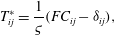 $$\begin{eqnarray}T_{ij}^{\ast }=\frac{1}{{\it\varsigma}}(FC_{ij}-{\it\delta}_{ij}),\end{eqnarray}$$
where
 $$\begin{eqnarray}F=\frac{L^{2}-3}{L^{2}-C_{kk}},\end{eqnarray}$$
is the Peterlin function and
 $L$
is related to the maximum extensibility of the polymer chains
 $L^{2}=L_{max}^{2}+3$
. In the present configuration, the nonlinear-spring law influences the perturbation field in two ways: (i) a weakening of the base-state normal stress as
 $W/L$
increases (see appendix B) and (ii) a new form of stress perturbation,
 $$\begin{eqnarray}{\it\tau}_{ij}^{\ast }=\frac{F}{{\it\varsigma}}\biggl(\!c_{ij}+\underbrace{\frac{1}{L^{2}-C_{ll}}C_{ij}c_{kk}}_{{\mathcal{N}}}\!\biggr),\end{eqnarray}$$
which is labelled
 ${\mathcal{N}}$
. The full perturbation equations for the FENE-P fluid are provided in appendix B.
Vortical perturbations (top) induced by Gaussian wall bump (bottom) in a FENE-P channels with
 $L=100$
. Filled contours are the spanwise vorticity, lines are the streamfunction. (a)
 ${\it\alpha}_{l}=0.5$
with
 ${\it\beta}=0.5$
,
 $W=40$
,
 $R=1$
. (b)
 ${\it\alpha}_{l}=10$
with
 ${\it\beta}=0.5$
,
 $W=30$
,
 $R=1000$
.

Contours of polymer stretch perturbations,
 $c_{kk}/L^{2}$
, in Couette flow of a FENE-P fluid with
 $L=100$
. (a) Shallow channel with
 ${\it\alpha}_{l}=0.5$
,
 $W=40$
,
 $R=1$
,
 ${\it\beta}=0.5$
. (b) Deep channel with
 ${\it\alpha}_{l}=10$
,
 $W=30$
,
 $R=1000$
,
 ${\it\beta}=0.5$
. Lines are contours of the streamfunction.

Streamwise energy and enstrophy spectra for the FENE-P fluid are reported in figures 18 and 19 for a shallow and a deep channel respectively. Note that the parameter sets correspond to the Oldroyd-B cases considered in figures 13 and 16. For the largest extensibility,
 $L=1000$
, the results are indistinguishable from the Oldroyd-B cases. For the more realistic values,
 $L=\{50,100\}$
, the FENE-P results exhibit the same qualitative trends as the Oldroyd-B fluids. In the shallow-elastic flow (figure 18) the energy and enstrophy are damped slightly across the full range of wavenumbers. In the transcritical flow (figure 19), the kinematic amplification mechanism remains active across a band of wavenumbers. The spectra are similar in shape to the Oldroyd-B results, although the peak in both the energy and enstrophy spectra is shifted to higher wavenumbers.
In figure 20 the flow response to the Gaussian bump is reported for the flows examined in figures 18 and 19 for the realistic value
 $L=100$
. The important flow features from the Oldroyd-B results remain: in the shallow-elastic channel, the vorticity maximum is located at the upper wall and a weak secondary vortex is formed upstream of the bump. In the transcritical channel, there is a strong non-local response in the vorticity at the critical layer, which takes the form of stripes tipped forward with the shear.
Finally, the polymer stretch field associated with each flow is examined in figure 21. In the shallow-elastic flow, the polymer is most strongly stretched directly above the wall bump, while a small ‘jet’ of polymer stretch protrudes downstream along the lower wall. For the transcritical flow, the polymer is stretched in a thin region between the two induced vortices, as anticipated from the vorticity field.
6 Conclusion
The flow response to surface waviness in a viscoelastic Couette flow was examined using linear theory. For an Oldroyd-B fluid at high Weissenberg number, the induced vorticity perturbations can be classified using a phase diagram in a similar manner to the Newtonian problem (Charru & Hinch Reference Charru and Hinch2000). The viscoelastic phase diagram is parameterized by two quantities: the ratios of the channel depth and of the critical layer height to the length scale of the surface undulation,
 ${\it\alpha}\equiv k^{\ast }d$
and
 ${\it\Sigma}\equiv k^{\ast }\sqrt{2{\it\nu}_{p}{\it\varsigma}}$
.
The phase diagram was divided in three regions: (i) when
 ${\it\alpha}<1$
and
 ${\it\Sigma}>{\it\alpha}$
, the flow is termed ‘shallow elastic’; the surface waves are long relative to the channel depth and the critical layer is outside of the flow domain. The bulk flow response is a constant vorticity generated by a distortion of the highly tensioned mean-flow streamlines. There is a substantial spanwise vorticity generated in a solvent boundary layer at the top wall where the flow adjusts to satisfy the top boundary conditions. (ii) When
 ${\it\alpha}>1$
and
 ${\it\Sigma}\gtrsim 1$
, the flow is labelled ‘deep elastic’; neither the top wall or the critical layer influence the perturbation field. The vortical perturbations are not affected by the elasticity in this regime. (iii) When
 ${\it\alpha}>{\it\Sigma}$
and
 ${\it\Sigma}\lesssim 1$
, the critical layer is inside the flow domain, and lies within one wavelength from the lower wall. This behaviour is termed ‘transcritical’, and is characterized by generation of vorticity at the critical layer, which is driven by a kinematic amplification mechanism for the polymer torque.
The analysis of a single wall wavelength was followed by a computational study of the flow response to localized disturbances using Fourier superposition. In shallow-elastic flows, the large vorticity generated at the upper wall leads to the formation of a second vortex upstream of the bump. In deep channels a significant vorticity is generated at the critical layer, and this has attached an associate pair of counter-rotating vortices. Calculations of the flow response to isolated bumps using the more realistic FENE-P model showed the same qualitative behaviour in both shallow and deep channels.
Future work should extend the analysis to finite-amplitude wall roughness, where the secondary instability of the curved streamlines in shallow channels may present a pathway to elastic turbulence. The influence of wall undulations on drag-reduced turbulent flows at high Reynolds numbers is also of interest since, in that regime, critical layers can be established in close proximity to the lower wall.
Acknowledgement
This work is sponsored by the Engineering and Physical Sciences Research Council and by the National Science Foundation under grant no. 1511937.
Appendix A. Further details on the transcritical regime
A.1 Solution of the elastic-Rayleigh equation
In the bulk of the channel, the streamfunction satisfies the elastic-Rayleigh equation,
 $$\begin{eqnarray}\frac{\text{d}^{2}}{\text{d}y^{2}}\left(\frac{{\it\psi}_{0}}{y}\right)+\frac{2y}{(y^{2}-{\it\Sigma}^{2})}\frac{\text{d}}{\text{d}y}\left(\frac{{\it\psi}_{0}}{y}\right)-k^{2}\left(\frac{{\it\psi}_{0}}{y}\right)=0.\end{eqnarray}$$
A solution is sought in the form of a Frobenius series about
 $y={\it\Sigma}$
(Bender & Orszag Reference Bender and Orszag1978) and takes the form,
 $$\begin{eqnarray}{\it\psi}_{0}^{\pm }(y)=A_{0}^{\pm }y\mathop{\sum }_{j=0}^{\infty }b_{j}(y-{\it\Sigma})^{j}+B_{0}^{\pm }y\left(\mathop{\sum }_{j=1}^{\infty }c_{j}(y-{\it\Sigma})^{j}+\mathop{\sum }_{j=0}^{\infty }b_{j}(y-{\it\Sigma})^{j}\log (y-{\it\Sigma})\right).\end{eqnarray}$$
The branch of the logarithm for
 ${\it\psi}_{0}^{-}(y)$
is chosen as
 $\text{log}(y-{\it\Sigma})=\text{log}|y-{\it\Sigma}|-\text{i}{\rm\pi}$
. The series coefficients in (A 2) are
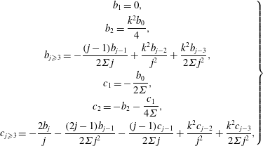 $$\begin{eqnarray}\displaystyle \left.\begin{array}{@{}c@{}}\displaystyle b_{1}=0,\\ \displaystyle b_{2}=\frac{k^{2}b_{0}}{4},\\ \displaystyle b_{j\geqslant 3}=-\frac{(j-1)b_{j-1}}{2{\it\Sigma}j}+\frac{k^{2}b_{j-2}}{j^{2}}+\frac{k^{2}b_{j-3}}{2{\it\Sigma}j^{2}},\\ \displaystyle c_{1}=-\frac{b_{0}}{2{\it\Sigma}},\\ \displaystyle c_{2}=-b_{2}-\frac{c_{1}}{4{\it\Sigma}},\\ \displaystyle c_{j\geqslant 3}=-\frac{2b_{j}}{j}-\frac{(2j-1)b_{j-1}}{2{\it\Sigma}j^{2}}-\frac{(j-1)c_{j-1}}{2{\it\Sigma}j}+\frac{k^{2}c_{j-2}}{j^{2}}+\frac{k^{2}c_{j-3}}{2{\it\Sigma}j^{2}},\end{array}\right\} & & \displaystyle\end{eqnarray}$$
where
 $b_{0}=1$
and
 $c_{0}=0$
.
Close to the critical layer the solution (A 2) is expressed in terms of the critical layer coordinate
 ${\it\eta}\equiv (y-{\it\Sigma})/{\it\delta}_{c}$
and the leading terms are,
 $$\begin{eqnarray}\displaystyle & \displaystyle {\it\psi}_{0}^{+}({\it\eta})\sim A_{0}^{+}{\it\Sigma}+B_{0}^{+}{\it\Sigma}(\text{log}|{\it\eta}|+\text{log}{\it\delta}_{c})+O({\it\delta}_{c}), & \displaystyle\end{eqnarray}$$
 $$\begin{eqnarray}\displaystyle & \displaystyle {\it\psi}_{0}^{-}({\it\eta})\sim A_{0}^{-}{\it\Sigma}+B_{0}^{-}{\it\Sigma}(\text{log}|{\it\eta}|-\text{i}{\rm\pi}+\text{log}{\it\delta}_{c})+O({\it\delta}_{c}). & \displaystyle\end{eqnarray}$$
 $$\begin{eqnarray}\overline{{\it\psi}}({\it\eta})=\log {\it\delta}_{c}\overline{{\it\psi}}_{-1}({\it\eta})+\overline{{\it\psi}}_{0}({\it\eta})+\cdots .\end{eqnarray}$$
The equations satisfied by the inner variable
 $\overline{{\it\psi}}({\it\eta})={\it\psi}(y)$
are solved below.
A.2 Solution in the critical layer
In the critical layer the balance between advection, polymer force generated by
 $T_{11}$
and solvent diffusion leads to
 $$\begin{eqnarray}\frac{\text{d}^{4}\overline{{\it\psi}}_{i}}{\text{d}{\it\eta}^{4}}-\frac{\text{d}}{\text{d}{\it\eta}}\left(\text{i}{\it\eta}\frac{\text{d}\overline{{\it\psi}}_{i}}{\text{d}{\it\eta}}\right)=0,\end{eqnarray}$$
where
 ${\it\eta}\equiv (y-{\it\Sigma})/{\it\delta}_{c}({\it\varepsilon})$
is the shifted coordinate scaled by the viscous length scale in the solvent,
 ${\it\delta}_{c}=({\it\varepsilon}{\it\beta}{\it\Sigma}^{2}/4\dot{{\it\gamma}}k(1-{\it\beta}))^{1/3}$
. Note that this equation is satisfied by the
 $O(\log {\it\delta}_{c})$
eigensolution,
 $\overline{{\it\psi}}_{-1}({\it\eta})$
and the
 $O(1)$
component,
 $\overline{{\it\psi}}_{0}({\it\eta})$
. Solutions are sought in the form of Laplace contour integrals,
 $$\begin{eqnarray}\overline{{\it\psi}}_{i}({\it\eta})=\int _{C}f({\it\zeta})\text{e}^{{\it\eta}{\it\zeta}}\,\text{d}{\it\zeta},\end{eqnarray}$$
where
 $C$
is a yet unspecified contour in the complex-
 ${\it\zeta}$
plane.
Possible integration contours in the complex
 ${\it\zeta}$
-plane that define the linearly independent solutions of (A 6).

Substituting (A 7) into (A 6) and differentiating under the integral sign,
 $$\begin{eqnarray}\int _{C}({\it\zeta}^{4}-\text{i}{\it\eta}{\it\zeta}^{2}-\text{i}{\it\zeta})f({\it\zeta})\text{e}^{{\it\eta}{\it\zeta}}\,\text{d}{\it\zeta}=0.\end{eqnarray}$$
Integrating by parts yields,
 $$\begin{eqnarray}\int _{C}\left[\left({\it\zeta}^{4}+\text{i}{\it\zeta}\right)f+\text{i}{\it\zeta}^{2}\frac{\text{d}f}{\text{d}{\it\zeta}}\right]\text{d}{\it\zeta}-\underbrace{\text{i}{\it\zeta}^{2}f({\it\zeta})\text{e}^{{\it\eta}{\it\zeta}}\bigg|_{C}}_{}=0,\end{eqnarray}$$
where the term identified with an underbrace is evaluated at the end points of the contour. After solving for
 $f({\it\zeta})$
, linearly independent solutions for the streamfunction are
 $$\begin{eqnarray}\overline{{\it\psi}}_{i}^{j}({\it\eta})=\int _{C_{j}}\left(\frac{1}{{\it\zeta}}\right)\text{exp}\left(\frac{\text{i}{\it\zeta}^{3}}{3}+{\it\eta}{\it\zeta}\right)\text{d}{\it\zeta},\end{eqnarray}$$
where the contours
 $C_{j}$
must satisfy
 $$\begin{eqnarray}{\it\zeta}\text{exp}\left(\frac{\text{i}{\it\zeta}^{3}}{3}+{\it\eta}{\it\zeta}\right)\bigg|_{C_{j}}=0.\end{eqnarray}$$
Valid integration contours are illustrated in figure 22. Contours can encircle the origin. They may also start and end at the origin or in one of the sectors in which
 $\text{exp}(\text{i}{\it\zeta}^{3}/3)$
is decaying at
 ${\it\zeta}\rightarrow \infty$
, which are indicated in grey in figure 22. Each contour yields a solution of (A 6), but four contours may not be chosen arbitrarily. For example, contours
 $C_{0}$
,
 $C_{1}$
,
 $C_{2}$
and
 $C_{3}$
do not produce four independent solutions, since
 $C_{1}$
,
 $C_{2}$
and
 $C_{3}$
can be joined at infinity to produce
 $C_{0}$
.
Numerically satisfactory solutions can be constructed using integration contours
 $C_{i};\;i\in [0,4,5,6]$
. The integration around
 $C_{0}$
encloses a simple pole, and the solution is a constant. The other paths are parameterized with
 ${\it\zeta}=s\text{e}^{\text{i}{\it\theta}}$
, with
 ${\it\theta}=\{{\rm\pi}/6,5{\rm\pi}/6,3{\rm\pi}/2\}$
. The solution is therefore
 $$\begin{eqnarray}\displaystyle \overline{{\it\psi}}_{i}({\it\eta}) & = & \displaystyle \overline{A}_{i}+\overline{B}_{i}\int _{{\it\sigma}}^{\infty }\left(\frac{1}{s}\right)\text{exp}\left(-\frac{s^{3}}{3}-\text{i}s{\it\eta}\right)\text{d}s\nonumber\\ \displaystyle & & \displaystyle +\,\overline{C}_{i}\int _{{\it\sigma}}^{\infty }\left(\frac{1}{s}\right)\text{exp}\left(-\frac{s^{3}}{3}+\frac{s{\it\eta}(\sqrt{3}+\text{i})}{2}\right)\text{d}s\nonumber\\ \displaystyle & & \displaystyle +\,\overline{D}_{i}\int _{{\it\sigma}}^{\infty }\left(\frac{1}{s}\right)\text{exp}\left(-\frac{s^{3}}{3}+\frac{s{\it\eta}(-\sqrt{3}+\text{i})}{2}\right)\text{d}s.\end{eqnarray}$$
These expressions are valid in the limit
 ${\it\sigma}\rightarrow 0$
. This limit results in divergent integrals in (A 12). The constant
 $\overline{A}_{i}$
can eliminate this effect, and this becomes apparent when (A 12) is matched to the elastic-Rayleigh equation below. For now, the dependence on
 ${\it\sigma}$
is retained, and the limit
 ${\it\sigma}\rightarrow 0$
will be taken once the unknown constants have been determined.
A.3 Matching with the elastic-Rayleigh equation
Discarding solutions which are exponentially growing as
 ${\it\eta}\rightarrow \pm \infty$
, the critical layer streamfunction is,
 $$\begin{eqnarray}\overline{{\it\psi}}_{i}({\it\eta})=\overline{A}_{i}+\overline{B}_{i}\int _{{\it\sigma}}^{\infty }\left(\frac{1}{s}\right)\text{exp}\left(-\frac{s^{3}}{3}-\text{i}s{\it\eta}\right)\text{d}s.\end{eqnarray}$$
In order to match this expression to the elastic-Rayleigh solutions in the bulk of the channel we examine the integral in the limits
 ${\it\eta}\rightarrow \pm \infty$
. Here we provide details of the limit
 ${\it\eta}\rightarrow \infty$
.
The integral in (A 13) is highly oscillatory as
 ${\it\eta}\rightarrow \infty$
. In order to obtain approximate expressions in this limit we use the method of steepest descent and deform the integration contour so that the phase in the exponent is constant (Bender & Orszag Reference Bender and Orszag1978). The dominant contributions to the integral in the limit
 ${\it\eta}\rightarrow \infty$
then come from regions of maximum altitude or saddle points.
The exponent in the integral in (A 13) has moveable saddle points in the complex
 $s$
-plane. Therefore, the change of variable
 $s=\sqrt{{\it\eta}}{\it\vartheta}$
is adopted. The integral to be approximated may then be written
 $$\begin{eqnarray}I({\it\lambda})=\int _{{\it\sigma}{\it\lambda}^{-1/3}}^{\infty }\frac{\text{e}^{{\it\lambda}g({\it\vartheta})}\text{d}{\it\vartheta}}{{\it\vartheta}},\end{eqnarray}$$
where
 ${\it\lambda}\equiv {\it\eta}^{3/2}$
and
 $g({\it\vartheta})=-{\it\vartheta}^{3}/3-\text{i}{\it\vartheta}$
.
Contours of the altitude
 $\mathscr{A}$
(colours and dashed lines) and phase
 $\mathscr{P}$
(solid lines) of the function
 $g({\it\vartheta})$
. The original integration contour,
 $L_{0}$
, is identified with the white dashed line. The solid white lines are those on which the phase
 $\mathscr{P}=-{\it\sigma}{\it\lambda}^{-1/3}$
and
 $\mathscr{P}=-\sqrt{2}/3$
and the labels
 $L_{1}$
and
 $L_{2}$
identify the path of steepest descent.

Contours of both the altitude,
 $\mathscr{A}({\it\vartheta})\equiv \text{Re}(g({\it\vartheta}))$
, and phase,
 $\mathscr{P}({\it\vartheta})\equiv \text{Im}(g({\it\vartheta}))$
, are plotted in figure 23 in the complex-
 ${\it\vartheta}$
plane. The original integration contour,
 $L_{0}$
, is along the real axis. The contour is deformed such onto
 $L_{1}+L_{2}$
, along each of which
 $\mathscr{P}=\text{constant}$
. The steepest descent paths
 $L_{1}$
and
 $L_{2}$
meet as
 ${\it\vartheta}\rightarrow \infty$
. Along
 $L_{1}$
the phase
 $\mathscr{P}=-{\it\sigma}{\it\lambda}^{-1/3}$
, while along
 $L_{2}$
the phase
 $\mathscr{P}=-\sqrt{2}/3$
.
The dominant contributions to the integral
 $I({\it\lambda})$
as
 ${\it\lambda}\rightarrow \infty$
are from the saddle point on
 $L_{2}$
and the end point
 ${\it\vartheta}={\it\sigma}{\it\lambda}^{-1/3}$
on
 $L_{1}$
, which is the point of maximum altitude. The contribution from the saddle point is exponentially small in comparison to the end point contribution, and is not presented here. At the end point the path,
 $L_{1}$
is parameterized,
 ${\it\vartheta}-{\it\sigma}{\it\lambda}^{-1/3}=r\text{e}^{\text{i}{\it\theta}}$
. As
 ${\it\lambda}\rightarrow \infty$
the exponent
 $g({\it\vartheta})$
may thus be approximated,
 $$\begin{eqnarray}\displaystyle g({\it\vartheta}) & {\approx} & \displaystyle -\frac{{\it\sigma}^{3}}{3{\it\lambda}}-\frac{\text{i}{\it\sigma}}{{\it\lambda}^{1/3}}+\left(-\frac{{\it\sigma}^{2}}{{\it\lambda}^{2/3}}-\text{i}\right)r\text{e}^{\text{i}{\it\theta}}+\cdots ,\nonumber\\ \displaystyle & {\approx} & \displaystyle -r-\frac{\text{i}{\it\sigma}}{{\it\lambda}^{1/3}}.\end{eqnarray}$$
The approximation to
 $I({\it\lambda})$
is therefore,
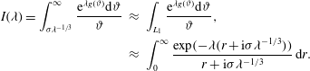 $$\begin{eqnarray}\displaystyle I({\it\lambda})=\int _{{\it\sigma}{\it\lambda}^{-1/3}}^{\infty }\frac{\text{e}^{{\it\lambda}g({\it\vartheta})}\text{d}{\it\vartheta}}{{\it\vartheta}} & {\approx} & \displaystyle \int _{L_{1}}\frac{\text{e}^{{\it\lambda}g({\it\vartheta})}\text{d}{\it\vartheta}}{{\it\vartheta}},\nonumber\\ \displaystyle & {\approx} & \displaystyle \int _{0}^{\infty }\frac{\text{exp}(-{\it\lambda}(r+\text{i}{\it\sigma}{\it\lambda}^{-1/3}))}{r+\text{i}{\it\sigma}{\it\lambda}^{-1/3}}\,\text{d}r.\end{eqnarray}$$
With a change of variable this expression can be written as a generalized exponential integral (Abramowitz & Stegun Reference Abramowitz and Stegun1964),
 $$\begin{eqnarray}\displaystyle I({\it\lambda}) & {\approx} & \displaystyle \int _{\text{i}{\it\sigma}{\it\eta}}^{\infty }\frac{\text{e}^{-w}\,\text{d}w}{w},\nonumber\\ \displaystyle & = & \displaystyle E_{1}(\text{i}{\it\sigma}{\it\eta})=-{\it\gamma}-\frac{\text{i}{\rm\pi}}{2}-\log {\it\sigma}-\text{log}|{\it\eta}|-\mathop{\sum }_{j=1}^{\infty }\frac{(-1)^{j}(\text{i}{\it\sigma}{\it\eta})^{j}}{jj!},\end{eqnarray}$$
where
 ${\it\gamma}=0.5772\ldots \,$
is the Euler–Mascheroni constant. In the limit
 ${\it\sigma}\rightarrow 0$
the algebraic contribution can be ignored and the streamfunction as
 ${\it\eta}\rightarrow \infty$
is
 $$\begin{eqnarray}\overline{{\it\psi}}_{i}({\it\eta}\rightarrow \infty )\sim \overline{A}_{i}+\overline{B}_{i}\left(-{\it\gamma}-\frac{\text{i}{\rm\pi}}{2}-\log {\it\sigma}-\text{log}|{\it\eta}|\right).\end{eqnarray}$$
Similar considerations as
 ${\it\eta}\rightarrow -\infty$
result in
 $$\begin{eqnarray}\overline{{\it\psi}}_{i}({\it\eta}\rightarrow -\infty )\sim \overline{A}_{i}+\overline{B}_{i}\left(-{\it\gamma}+\frac{\text{i}{\rm\pi}}{2}-\log {\it\sigma}-\text{log}|{\it\eta}|\right).\end{eqnarray}$$
Matching these expressions to inner limit of the elastic-Rayleigh solutions (A 4) reveals
 $A_{0}^{+}=A_{0}^{-}\equiv A_{0}$
,
 $B_{0}^{+}=B_{0}^{-}\equiv B_{0}$
and determines the constants for the inner solution,
 $$\begin{eqnarray}\displaystyle \overline{{\it\psi}}({\it\eta}) & = & \displaystyle {\it\Sigma}B_{0}\log {\it\delta}_{c}+{\it\Sigma}A_{0}+{\it\Sigma}B_{0}\left(-{\it\gamma}-\frac{\text{i}{\rm\pi}}{2}-\log {\it\sigma}\right)\nonumber\\ \displaystyle & & \displaystyle -\,{\it\Sigma}B_{0}\int _{{\it\sigma}}^{\infty }\left(\frac{1}{s}\right)\text{exp}\left(-\frac{s^{3}}{3}-\text{i}s{\it\eta}\right)\text{d}s.\end{eqnarray}$$
In the limit
 ${\it\sigma}\rightarrow 0$
the logarithmic term regularizes the lower limit of the integral.
Appendix B. Flow equations for a FENE-P fluid
B.1 Base state
In a FENE-P fluid the polymer stress is related to the conformation tensor through a nonlinear-spring law,
 $$\begin{eqnarray}\unicode[STIX]{x1D61B}_{ij}=\frac{1}{W}(FC_{ij}-{\it\delta}_{ij}),\end{eqnarray}$$
where
 $F$
is the Peterlin function,
 $$\begin{eqnarray}F=\frac{L^{2}-3}{L^{2}-C_{kk}}.\end{eqnarray}$$
In simple shear,
 $U=\dot{{\it\gamma}}y$
, the base-state polymer stresses for a FENE-P fluid can be related to the Oldroyd-B values (Sureshkumar, Beris & Handler Reference Sureshkumar, Beris and Handler1997),
 $$\begin{eqnarray}\frac{T_{11}}{T_{11}^{\infty }}=\frac{1}{F^{2}},\quad \frac{T_{12}}{T_{12}^{\infty }}=\frac{1}{F},\end{eqnarray}$$
where the superscript
 $\infty$
identifies the Oldroyd-B result. The Peterlin function depends on the parameter
 ${\it\varrho}\equiv \dot{{\it\gamma}}W/L$
,
 $$\begin{eqnarray}F({\it\varrho})=\frac{\sqrt{6}{\it\varrho}}{2\text{sinh}(q/3)},\quad \text{with }q=\text{sinh}^{-1}(3\sqrt{6}{\it\varrho}/2).\end{eqnarray}$$
The function
 $F$
is monotonically decreasing with increasing
 ${\it\varrho}$
(Ray & Zaki Reference Ray and Zaki2014). Therefore, the polymer stresses are always attenuated by finite extensibility. For the parameters of interest in this paper,
 ${\it\varrho}=O(1)$
and the Oldroyd-B scaling remains,
 $T_{11}=O(W\dot{{\it\gamma}}^{2})$
,
 $T_{12}=O(\dot{{\it\gamma}})$
(Page & Zaki Reference Page and Zaki2015).
B.2 Linear perturbation equations
The continuity and momentum equations are,
 $$\begin{eqnarray}\displaystyle & \displaystyle \text{i}ku+\frac{\text{d}v}{\text{d}y}=0, & \displaystyle\end{eqnarray}$$
 $$\begin{eqnarray}\displaystyle & \displaystyle \text{i}k\dot{{\it\gamma}}yu+\dot{{\it\gamma}}v=-\text{i}kp+\frac{{\it\alpha}^{2}}{R}\left[{\it\beta}\left(\frac{\text{d}^{2}}{\text{d}y^{2}}-k^{2}\right)u+(1-{\it\beta})\left(\text{i}k{\it\tau}_{11}+\frac{\text{d}{\it\tau}_{12}}{\text{d}y}\right)\right], & \displaystyle\end{eqnarray}$$
 $$\begin{eqnarray}\displaystyle & \displaystyle \text{i}k\dot{{\it\gamma}}yv=-\frac{\text{d}p}{\text{d}y}+\frac{{\it\alpha}^{2}}{R}\left[{\it\beta}\left(\frac{\text{d}^{2}}{\text{d}y^{2}}-k^{2}\right)v+(1-{\it\beta})\left(\text{i}k{\it\tau}_{12}+\frac{\text{d}{\it\tau}_{22}}{\text{d}y}\right)\right]. & \displaystyle\end{eqnarray}$$
 $$\begin{eqnarray}{\it\tau}_{ij}=\frac{F}{W}\left(c_{ij}+\frac{1}{L^{2}-C_{ll}}C_{ij}c_{kk}\right).\end{eqnarray}$$
The relevant components of the conformation tensor evolve according to,
 $$\begin{eqnarray}\displaystyle & \displaystyle \text{i}k\dot{{\it\gamma}}yc_{11}+\frac{1}{W}{\it\tau}_{11}=2\text{i}kC_{11}u+2C_{12}\frac{\text{d}u}{\text{d}y}+2\dot{{\it\gamma}}c_{12}, & \displaystyle\end{eqnarray}$$
 $$\begin{eqnarray}\displaystyle & \displaystyle \text{i}k\dot{{\it\gamma}}yc_{12}+\frac{1}{W}{\it\tau}_{12}=\text{i}kC_{11}v+C_{22}\frac{\text{d}u}{\text{d}y}+\dot{{\it\gamma}}c_{22}, & \displaystyle\end{eqnarray}$$
 $$\begin{eqnarray}\displaystyle & \displaystyle \text{i}k\dot{{\it\gamma}}yc_{22}+\frac{1}{W}{\it\tau}_{22}=2\text{i}kC_{12}v+2C_{22}\frac{\text{d}v}{\text{d}y}, & \displaystyle\end{eqnarray}$$
 $$\begin{eqnarray}\displaystyle & \displaystyle \text{i}k\dot{{\it\gamma}}yc_{33}+\frac{1}{W}{\it\tau}_{33}. & \displaystyle\end{eqnarray}$$