



1. Introduction
Fluid-driven fracture propagation is a typical moving-boundary problem that governs mass transport, energy release and the structural evolution of permeable media. The dynamic coupling between viscous fluid flow and solid deformation plays a central role in a wide spectrum of natural and engineered systems. In nature, such processes control the emplacement of magma dikes (Spence & Turcotte Reference Spence and Turcotte1985; Spence et al. Reference Spence, Sharp and Turcotte1987; Lister Reference Lister1990b
; Rubin Reference Rubin1998), the propagation of crevasses in glaciers (Tsai & Rice Reference Tsai and Rice2010) and the formation of natural hydraulic fractures (Renshaw & Harvey Reference Renshaw and Harvey1994; Berchenko et al. Reference Berchenko, Detournay and Chandler1997; Liu et al. Reference Liu, Zhang and Detournay2025b
). Concurrently, in subsurface engineering, understanding these coupled fluid-mechanical dynamics is essential for advancing energy transition technologies, including CO
 $_2$
sequestration (Fu et al. Reference Fu, Settgast, Hao, Morris and Ryerson2017; Han et al. Reference Han, Shi, Ni, Zhang and Gao2024; Zhang et al. Reference Zhang, Zhang, Song, Wei, Liu and Wang2025), underground energy storage (Yuan et al. Reference Yuan, Wood and Yu2015; Wang et al. Reference Wang, Jie, Zhou and Ma2024; Hu & Wang Reference Hu and Wang2024) and enhanced geothermal systems (Niemz et al. Reference Niemz, McLennan, Pankow, Rutledge and England2024; Singh et al. Reference Singh, Galban, McClure, Briggs and Norbeck2025), as well as conventional hydrocarbon recovery (King Reference King2010, Reference King2012; Economides Reference Economides2013).
To understand and predict such processes, classical theoretical models have been developed since the mid-20th century, including the plane strain or Khristianovic–Geertsma–de Klerk (KGD) (Khristianovic & Zheltov Reference Khristianovic and Zheltov1955; Geertsma & De Klerk Reference Geertsma and De Klerk1969), constant height or Perkins–Kern–Nordgren (PKN) (Perkins & Kern Reference Perkins and Kern1961; Nordgren Reference Nordgren1972) and penny-shaped or radial formulations, as well as extensions to three-dimensional (3-D) or planar geometries, such as pseudo-3-D models (Cleary Reference Cleary1980; Adachi et al. Reference Adachi, Detournay and Peirce2010; Dontsov & Peirce Reference Dontsov and Peirce2015; Nguyen et al. Reference Nguyen, Lee and Elraies2022) and planar-3-D/full-3-D models (Cleary et al. Reference Cleary, Kavvadas and Lam1983; Settari & Cleary Reference Settari and Cleary1984; Vandamme & Curran Reference Vandamme and Curran1989; Siebrits & Peirce Reference Siebrits and Peirce2002). These classical formulations, often combined with Carter’s leak-off law, have established a consistent theoretical framework for classifying fracture propagation regimes or limiting solutions. In particular, the classical
 $M\tilde {M}K\tilde {K}$
parametric space (Detournay Reference Detournay2016) organizes the asymptotic behaviour in terms of the dominant dissipation mechanism, namely viscosity or toughness, together with the relative roles of fracture storage and leak-off. This framework has supported the development of numerous analytical and semianalytical solutions across various geometries (Adachi Reference Adachi2001; Madyarova Reference Madyarova2003; Hu & Garagash Reference Hu and Garagash2010; Dontsov Reference Dontsov2017; Dontsov Reference Dontsov2016a
, Reference Dontsov2022), as well as extensions to non-Newtonian fluids (Dontsov Reference Dontsov2019; Kanin et al. Reference Kanin, Dontsov, Garagash and Osiptsov2021) and pressure-dependent leak-off (Kanin et al. Reference Kanin, Dontsov, Garagash and Osiptsov2020a
,
Reference Kanin, Garagash and Osiptsovb
). While these classical paradigms remain the foundation of modern fracture theory, they typically neglect the two-way poroelastic coupling between the leaking fluid and the surrounding matrix. Fluid leak-off from the fracture perturbs the pore-pressure field in the surrounding formation. The associated pore-pressure increase induces poroelastic deformation of the rock matrix and generates a compressive normal stress acting on the fracture faces. This stress, referred to here as poroelastic backstress, opposes fracture opening. It is expected to become relevant when its magnitude is comparable to the pressure scales associated with the classical viscous, toughness or leak-off-dominated regimes. Under such conditions, the classical regime structure can be altered, motivating the introduction of the backstress-dominated vertex in the regime map.
With the advancement of numerical methods, many studies have extended hydraulic fracture modelling to fully coupled poroelastic formulations using numerical methods such as the finite element method (Salimzadeh et al. Reference Salimzadeh, Paluszny and Zimmerman2017; Golovin & Baykin Reference Golovin and Baykin2018; Baykin & Golovin Reference Baykin and Golovin2018; Baykin et al. Reference Baykin, Abdullin, Dontsov and Golovin2023; Liu et al. Reference Liu, Dontsov, He and Zhang2025a ), extended finite element method (Mohammadnejad & Andrade Reference Mohammadnejad and Andrade2016; Wang et al. Reference Wang, Liu, Zeng, Gao and Zhuang2017; Vahab & Khalili Reference Vahab and Khalili2018; Luo et al. Reference Luo, Zhang, Zhao, Zeng, Liu and Li2020), phase-field method (Mikelić et al. Reference Mikelić, Wheeler and Wick2015; Santillán et al. Reference Santillán, Juanes and Cueto-Felgueroso2018; You & Yoshioka Reference You and Yoshioka2023; Liu et al. Reference Liu, Yoshioka, You, Li and Zhang2024), discrete approaches (Grassl et al. Reference Grassl, Fahy, Gallipoli and Wheeler2015) and boundary element or displacement discontinuity approaches coupled with diffusion equations (Kovalyshen Reference Kovalyshen2010; Kovalyshen & Detournay Reference Kovalyshen and Detournay2013; Rezaei et al. Reference Rezaei, Siddiqui, Bornia and Soliman2019). These models can accurately capture the spatiotemporal evolution of pore pressure and the resulting poroelastic stresses, providing detailed descriptions of fracture-rock interaction, stress shadowing and multifracture interference. However, their mathematical and computational complexity, together with the slow numerical convergence of coupled simulations, makes theoretical analysis difficult and often precludes systematic parametric or asymptotic studies that are essential for identifying the dominant processes that occur during hydraulic fracturing.
The aim of this study is to bridge the gap between the analytical simplicity of classical hydraulic fracture models and the physical complexity of fully coupled poroelastic simulations. Building on a previously developed simplified poroelastic formulation for hydraulic fractures that captures the essential feedback between pore-pressure diffusion and elastic deformation (Dontsov Reference Dontsov2021), we investigate how leak-off-induced backstress modifies the asymptotic evolution of plane-strain, radial and constant-height fractures. These geometries represent canonical cases and are widely used in both engineering applications and scientific research. The plane-strain geometry is relevant as an early-time approximation for fractures propagating from vertical wells. The radial geometry describes axisymmetric propagation in the absence of confining geological layers. The constant-height geometry represents fractures confined between bounding layers above and below the propagation plane. These geometries also provide reference solutions for laboratory experiments and numerical simulations, with the plane-strain geometry serving as a benchmark for two-dimensional models and the radial and constant-height geometries for 3-D models (Bunger & Detournay Reference Bunger and Detournay2008; Lecampion et al. Reference Lecampion, Bunger and Zhang2018; Zia & Lecampion Reference Zia and Lecampion2020). Within this framework, we derive the backstress-dominated self-similar limit, incorporate it into the classical parametric-space description, and examine transition solutions connecting the classical limiting regimes to this new regime. Although the present formulation is developed for fluid-driven fractures in poroelastic media, an analogous diffusion-induced stress mechanism also arises in thermoelastic problems, where temperature diffusion generates thermoelastic stresses. This, for instance, occurs in geothermal systems (Detournay & Cheng Reference Detournay and Cheng1993; Cheng Reference Cheng2016).
The remainder of the paper is organized as follows. Section 2 presents the governing equations and the simplified poroelastic framework for a general planar hydraulic fracture, and outlines the assumptions of the model. Sections 3–5 analyse three different fracture geometries, namely, plane strain, radial and constant height hydraulic fractures. For each of the geometries, an analytical solution for the backstress-dominated limit (or
 $B$
vertex) is obtained, a parametric space is constructed to specify the location of this new limit relative to the existing
 $M\tilde {M}K\tilde {K}$
vertices, and finally transitions to the
 $B$
-vertex solution are investigated. Section 6 discusses some of the applications and applicability of the developed framework and the
 $B$
-vertex solution. Finally, § 7 summarizes the main findings and conclusions of the study.
2. Simplified model for a planar fluid-driven fracture with poroelastic backstress
Consider the problem of a single planar hydraulic fracture propagating in a homogeneous poroelastic formation, as shown in figure 1. Let the fracture occupy the
 $ (x,y )$
plane, so that the fracture opening is in the
 $z$
direction. To account for the effect of poroelastic backstress, we follow the approach proposed in Dontsov (Reference Dontsov2021), in which case the governing equations can be written as
 \begin{align} & \frac {\partial w}{\partial t}+\boldsymbol{\nabla }\boldsymbol{\cdot }q+\frac {C^{\prime }}{\sqrt {t-t_{0}(x,y)}}=Q_{0}\delta (x,y),\quad q=-\frac {w^{3}}{\mu ^{\prime }}\boldsymbol{\nabla }p_{f}, \nonumber\\ & p_{f}=\sigma _{0}-\frac {E^{\prime }}{8\pi }\int _{S}\frac {(w+w^{\ell o})\mathrm{d}x^{\prime }\mathrm{d}y^{\prime }}{[(x-x^{\prime })^{2}+(y-y^{\prime })^{2}]^{3/2}},\quad w^{\ell o}=2B^{\prime }C^{\prime }\sqrt {t-t_{0}(x,y)},\nonumber\\ & w=\frac {K^{\prime }}{E^{\prime }}s^{1/2},\quad s\rightarrow 0. \end{align}
The hypersingular elastic integral is understood in the Hadamard finite-part sense. Here the fracture is characterized by its width
 $w$
,
 $q$
is the fluid flux,
 $p_{f}$
is fluid pressure, while
 $t_0(x,y)$
is the time at which the fracture front reached the point
 $(x,y)$
. Also, the last equation represents the propagation condition, in which
 $s$
is the distance to the fracture front. The formation parameters are undrained Young’s modulus
 $E_u$
, undrained Poisson’s ratio
 $\nu _u$
, in situ stress
 $\sigma _0$
, fracture toughness
 $K_{Ic}$
, Carter’s leak-off coefficient
 $C_{\ell }$
, Biot coefficient
 $\alpha$
and Biot modulus
 $M$
(the last two affect the value of
 $B'$
). The additional dimensionless parameter
 $B'$
determines the magnitude of
 $w^{\ell o}$
. For saturated rocks, it can be estimated as
 \begin{align} B'=\frac {2\alpha (1-\nu _u)M}{P+\alpha ^2M}, \quad P=\frac {(1-\nu )E}{(1+\nu )(1-2\nu )}, \end{align}
where
 $E$
and
 $\nu$
are the drained elastic constants and
 $P$
is the drained P-wave modulus. This expression shows that
 $B'$
is typically of the order of one for saturated rocks. For unsaturated rocks,
 $B'$
is usually much smaller because it scales with the ratio between the internal fluid pressure and the elastic modulus. The detailed derivation and the unsaturated expression are given in Appendix A. All of these are assumed to be spatially homogeneous. The injection is located at the origin and has rate
 $Q_0$
; the injected fluid has viscosity
 $\mu$
.
To reduce the length of mathematical expressions, the following alternative parameters are defined:
 \begin{equation} E^{\prime }=\frac {E_u}{1-\nu _u^{2}},\quad K^{\prime }=4\sqrt {\frac {2}{\pi }}K_{Ic},\quad C^{\prime }=2C_{\ell },\quad \mu ^{\prime }=12\mu . \end{equation}
Note that the hydrostatic pressure gradient is not included for simplicity. The governing equations use the undrained elastic constants. Fracture toughness can be defined under drained or undrained conditions, and the relation between the corresponding toughness values depends on
 $E^{\prime }/E_d^{\prime }$
, where
 $E_d^{\prime }=E/(1-\nu ^2)$
. For either definition, the propagation condition in (2.1) can be expressed in the form used here by choosing the toughness value consistently with the elastic modulus.
The primary difference from the classical hydraulic fracturing equations that ignore the effect of poroelastic stress is an additional term
 $w^{\ell o}$
, which captures the effect of poroelasticity. The quantity
 $w^{\ell o}$
represents the leak-off-induced swelling of the formation normal to the fracture surface (Dontsov Reference Dontsov2021). It is not the mechanical fracture aperture, but an effective aperture used in the elastic boundary integral equation to account for the poroelastic normal stress acting on the fracture faces.
Sketch of a planar fluid-driven fracture: (a) planar view; (b) cross-section view. The grey region represents the surrounding formation, and the light-blue region schematically represents the pressure-diffusion zone around the fracture.

It is crucial to outline the main assumptions of the simplified model. This backstress model effectively utilizes similar assumptions as Carter’s leak-off model (Howard & Fast Reference Howard and Fast1957), whereby the size of the pressure diffusion zone around the fracture (indicated by
 $d$
in figure 1) is assumed to be much smaller than the fracture size. More specifically, the Carter-type approximation requires the fracture front to move faster than the pore-pressure diffusion wave. Another requirement of the model is that the fracture net pressure remains small relative to the leak-off driving pressure, i.e.
 $p_f - \sigma _0 \ll \sigma _0-p_0$
. In this case, the Carter leak-off coefficient can be treated as independent of the transient fracture pressure. These assumptions result in one-dimensional fluid flow in the direction perpendicular to the fracture and make the zone of the pressure perturbation around the fracture relatively thin, which simplifies calculations of the leak-off-induced stress. The model retains the hydraulic-to-mechanical effect of leak-off-induced pore-pressure diffusion through the poroelastic backstress, but neglects the reverse mechanical-to-hydraulic feedback, namely the effect of fracture-induced stress changes on the reservoir pore-pressure field. As discussed in Dontsov (Reference Dontsov2021), the pore pressure change due to mechanical-to-hydraulic coupling is of the order of fracture net pressure, which is much smaller than the stress difference
 $\sigma _0-p_0$
. The latter represents the magnitude of pressure perturbation caused by leak-off. As can be seen from the result (2.1), such assumptions lead to a very simple contribution of the leak-off induced poroelastic stress. Specifically, fluid leak-off causes swelling of the rock that is represented by an addition of an effective aperture
 $w^{\ell o}$
, whose magnitude is proportional to the total volume of leaked fluid. Although this representation is valid on the fracture plane, stress calculations outside the fracture plane differ for the actual fracture opening and the poroelastic stress. Therefore, the concept of effective aperture does not apply outside of the fracture plane for the purpose of stress calculations.
The governing equations (2.1) are written for a general planar hydraulic fracture. However, in order to perform the analysis, we further restrict ourselves to three specific fracture geometries. Namely, plane strain or KGD geometry (Khristianovic & Zheltov Reference Khristianovic and Zheltov1955; Geertsma & De Klerk Reference Geertsma and De Klerk1969), radially symmetric geometry and constant height or PKN geometry (Perkins & Kern Reference Perkins and Kern1961; Nordgren Reference Nordgren1972). All these cases feature a one-dimensional formulation and are amenable to analysis.
3. Plane-strain fracture
In this section, we analyse the problem of a plane strain hydraulic fracture with poroelastic backstress. The governing equations and the general scaling relations are presented first. The backstress-dominated
 $B$
-vertex is then derived. This, in turn, allows us to construct the parametric space that includes the influence of backstress and features the new
 $B$
-regime. Finally, some of the transition solutions are developed to connect the classical limiting regimes with the backstress-dominated regime.
3.1. Governing equations
The plane strain model (Khristianovic & Zheltov Reference Khristianovic and Zheltov1955; Geertsma & De Klerk Reference Geertsma and De Klerk1969) assumes that crack deformation and propagation occur in the state of plane strain, as shown in figure 2. The corresponding governing equations can be obtained from the planar model (2.1) by neglecting variation with respect to the vertical coordinate
 $y$
as
 \begin{align} & \frac {\partial w}{\partial t}+\frac {\partial q}{\partial x}+\frac {C^{\prime }}{\sqrt {t-t_{0}(x)}}=Q_{0}\delta (x),\quad q=-\frac {w^{3}}{\mu ^{\prime }}\frac {\partial p_{f}}{\partial x},\nonumber\\ & p=p_{f}-\sigma _{0}=-\frac {E^{\prime }}{4\pi }\int _{-\ell }^{\ell }\frac {w+w^{\ell o}}{(x-s)^{2}}\mathrm{d}s,\quad w^{\ell o}=2B^{\prime }C^{\prime }\sqrt {t-t_{0}(x)},\nonumber\\ & w=\frac {K^{\prime }}{E^{\prime }}(\ell -x)^{1/2},\quad x\rightarrow \ell ,\nonumber\\ & Q_{0}t=2\int _{0}^{\ell (t)}w(x,t)\mathrm{d}x+4C^{\prime }\int _{0}^{\ell (t)}\sqrt {t-t_{0}(x)}\mathrm{d}x. \end{align}
Here the net pressure is introduced as
 $p$
, the fracture half-length is
 $\ell$
and the global volume balance is also written for future reference, assuming a symmetric fracture.
Sketch of a plane strain fluid-driven fracture.

3.2. General scaling
To proceed with the analysis and to find self-similar solutions, we employ the following scaling:
 \begin{align} &x=\ell (t)\xi ,\quad \ell (t)=L(t)\gamma (t),\nonumber \\ &p_{f}(x,t)-\sigma _{0}=P(t)\varPi (\xi ,t),\quad w(x,t)=W(t)\varOmega (\xi ,t), \end{align}
where
 $L$
,
 $P$
,
 $W$
are time-dependent scales that need to be determined. By transforming the derivatives as
 \begin{equation} \left .\frac {\partial }{\partial x}\right |_{x}=\frac {1}{\ell }\left .\frac {\partial }{\partial \xi }\right |_{\xi },\quad \left .\frac {\partial }{\partial t}\right |_{x}=\left .\frac {\partial }{\partial t}\right |_{\xi }-\xi \frac {\dot {\ell }}{\ell }\frac {\partial }{\partial \xi }, \end{equation}
the governing equations (3.1) become
 \begin{align} & G_{v}\left [\frac {\dot {W}}{W}\varOmega t+\dot {\varOmega }t-\xi \left (\frac {\dot {\gamma }t}{\gamma }+\frac {\dot {L}t}{L}\right )\frac {\partial \varOmega }{\partial \xi }\right ]-\frac {1}{G_{m}}\frac {1}{\gamma ^{2}}\frac {\partial }{\partial \xi }\left (\varOmega ^{3}\frac {\partial \varPi }{\partial \xi }\right )+\frac {G_{c}}{\sqrt {1-\theta (\xi)}}=0,\nonumber\\ & \varPi =-\frac {G_{e}}{4\pi \gamma }\int _{-1}^{1}\frac {\varOmega (\zeta)}{(\xi -\zeta )^{2}}\mathrm{d}\zeta -\frac {G_{p}}{2\pi \gamma }\int _{-1}^{1}\frac {\sqrt {1-\theta (\zeta)}}{(\xi -\zeta )^{2}}\mathrm{d}\zeta ,\nonumber\\ & \varOmega =G_{k}\gamma ^{1/2}(1-\xi )^{1/2},\quad \xi \rightarrow 1,\nonumber\\ & \frac {1}{2\gamma }=G_{v}\int _{0}^{1}\varOmega \mathrm{d}\xi +2G_{c}\int _{0}^{1}\sqrt {1-\theta (\xi)}\mathrm{d}\xi , \end{align}
while the dimensionless groups are
 \begin{align} &G_{v}=\frac {WL}{Q_{0}t},\quad G_{m}=\frac {\mu ^{\prime }Q_{0}L}{W^{3}P},\quad G_{c}=\frac {C^{\prime }L}{Q_{0}t^{1/2}},\nonumber \\ &G_{e}=\frac {E^{\prime }W}{PL},\quad G_{p}=\frac {E^{\prime }B^{\prime }C^{\prime }t^{1/2}}{PL},\quad G_{k}=\frac {K^{\prime }L^{1/2}}{E^{\prime }W}. \end{align}
Note that the newly introduced backstress-related dimensionless group is related to other parameters as
 $G_{p}=B^{\prime }G_{e}{G_{c}}/{G_{v}}$
. The dimensionless group
 $G_v$
characterizes the fracture volume relative to the injected volume;
 $G_m$
captures the effect of fluid viscosity;
 $G_c$
quantifies leak-off volume relative to the injected volume;
 $G_e$
reflects the relation between the opening and the pressure;
 $G_p$
measures the influence of backstress;
 $G_k$
represents fracture toughness.
3.3. Backstress-dominated
 $B$
-vertex

Backstress inevitably accompanies the pore-pressure diffusion induced by leak-off. Formally, the
 $B$
-vertex scaling is defined by requiring
 $G_c$
,
 $G_e$
and
 $G_p$
to be of the order of one. These three conditions express the simultaneous leading-order balance between leak-off, elastic deformation and poroelastic backstress, while other terms are assumed to be subdominant. In the present formulation we set
 $G_c=G_e=G_p=1$
, which establishes the characteristic length, opening and pressure scales. This common definition of the
 $B$
-scaling is used for the plane-strain, radial and constant-height geometries, so that the resulting
 $B$
-vertices can be compared within the same physical balance. According to the result in (3.5), the corresponding scales are
 \begin{equation} L=\frac {Q_{0}t^{1/2}}{C^{\prime }},\quad W=B^{\prime }C^{\prime }t^{1/2},\quad P=\frac {E^{\prime }B^{\prime }C^{\prime 2}}{Q_{0}}. \end{equation}
The remaining dimensionless groups are
 \begin{equation} G_{v}=B^{\prime },\quad G_{m}=\frac {\mu ^{\prime }Q_{0}^{3}}{B^{\prime 4}E^{\prime }C^{\prime 6}t},\quad G_{k}=\frac {K^{\prime }Q_{0}^{1/2}}{B^{\prime }E^{\prime }C^{\prime 3/2}t^{1/4}}. \end{equation}
The storage group
 $G_v$
follows directly from the definitions in (3.5). For
 $t\to \infty$
, we have
 $G_{m}\rightarrow 0$
and
 $G_{k}\rightarrow 0$
, and therefore the corresponding terms are negligible in the
 $B$
-vertex. In this situation, given that the fracture length is proportional to
 $t^{1/2}$
(see (3.6)), the leak-off history is simplified to
 $\theta =t_{0}/t= (x/\ell )^{2}=\xi ^{2}$
, and the contribution of the back stress in the elasticity equation in (3.4) can be rewritten as
 \begin{equation} \varPi _b=-\frac {1}{2\pi \gamma }\int _{-1}^{1}\frac {\sqrt {1-\zeta ^{2}}}{(\xi -\zeta )^{2}}\mathrm{d}\zeta =\frac {1}{2\gamma }. \end{equation}
Since
 $G_{m}\rightarrow 0$
, the lubrication equation in (3.4) results in
 $\varPi =\mathrm{const}$
. Given the uniform pressure and constant contribution of the backstress, the elasticity equation in (3.4) can be solved for fracture width, which essentially represents a solution for a Griffith fracture (Sneddon & Elliot Reference Sneddon and Elliot1946). Expansion of the general solution for fracture opening
 $\varOmega =k\sqrt {1-\xi ^{2}}$
near the tip leads to
 \begin{equation} \varOmega =\sqrt {2}k(1-\xi )^{1/2},\quad \xi \rightarrow 1. \end{equation}
Comparison of this result with the propagation criterion in (3.4) leads to
 $k=G_{k}\gamma ^{1/2}/\sqrt {2}$
, and since
 $G_{k}\rightarrow 0$
, we have
 $\varOmega \rightarrow 0$
. The fracture length can be calculated from the global volume balance equation in (3.4) as
 $\gamma =1/\pi$
, while the pressure has only contribution of the backstress
 \begin{equation} \varPi =\varPi _b=\frac {\pi }{2}. \end{equation}
To summarize the above, the corresponding dimensionless self-similar solution for the backstress-dominated limit is
 \begin{equation} \varPi _{b0}=\frac {\pi }{2},\quad \varOmega _{b0}=0,\quad \gamma _{b0}=\frac {1}{\pi }, \end{equation}
which we refer to as the
 $B$
-vertex. The result
 $\varOmega _{b0}=0$
is a leading-order result in the
 $B$
-scaling. It indicates that no aperture of order
 $W_b=B'C't^{1/2}$
is resolved at the
 $B$
-vertex, rather than that the physical aperture is exactly zero. A finite aperture is recovered when the subdominant toughness or viscous contribution is retained in the transition problem, as is shown later in this section. By using the scaling relations (3.2) and (3.6), the dimensional form of the above solution is
 \begin{equation} p_{b0}=\frac {\pi }{2}\frac {E^{\prime }B^{\prime }C^{\prime 2}}{Q_{0}},\quad w_{b0}=o(B'C't^{1/2}),\quad \ell _{b0}=\frac {Q_{0}}{\pi C^{\prime }}t^{1/2}. \end{equation}
As can be seen from the result, in this limiting case or regime, the net pressure is balanced at leading order by the poroelastic backstress, so that no aperture is resolved at the
 $B$
-scaling. In addition, the fracture length is identical to that for the leak-off-dominated regimes that assume no backstress (Adachi & Detournay Reference Adachi and Detournay2008).
3.4. Parametric space
The next goal is to modify the existing parametric space for the considered plane-strain fracture geometry (Dontsov Reference Dontsov2017) and to introduce the effect of poroelastic backstress. The dimensionless variables that define the original diagram are
 \begin{equation} \tau =\frac {tE^{\prime }C^{\prime 6}}{\mu ^{\prime }Q_{0}^{3}},\quad K_{m}=\left (\frac {K^{\prime 4}}{\mu ^{\prime }E^{\prime 3}Q_{0}}\right )^{1/4}. \end{equation}
In the absence of backstress, there are four limiting regimes: storage-viscosity
 $M$
; leak-off-viscosity
 $\tilde {M}$
; storage-toughness
 $K$
; leak-off-toughness
 $\tilde {K}$
. The presence of backstress adds an additional backstress-dominated regime or
 $B$
-vertex, which is defined in the previous section.
In contrast to the approach in Dontsov (Reference Dontsov2017), in which an approximate solution is used to determine boundaries of fracture regimes, we are going to utilize an alternative approach that uses only vertex solutions. While the latter approach is simpler, it is much less accurate and provides only an approximate result. Such an approach was also adopted in Dontsov (Reference Dontsov2019). Nevertheless, this is the only option at this point since all the vertex solutions are known, while the approximate solution for the whole parametric space is currently unavailable. Specifically, to construct the parametric space, the following metric is used:
 \begin{equation} p_{i0}=\epsilon p_{j0}\left (\frac {\ell }{2},t\right ),\quad \epsilon p_{i0}=p_{j0}\left (\frac {\ell }{2},t\right ), \end{equation}
where subscripts
 $i$
and
 $j$
(
 $i\neq j$
) correspond to
 $M$
,
 $\tilde {M}$
,
 $K$
,
 $\tilde {K}$
and
 $B$
vertex solutions. The tolerance parameter
 $\epsilon$
is specified below through the calibration procedure used to construct the approximate parametric space. Given two individual regimes
 $i$
and
 $j$
, (3.14) allow us to calculate the boundaries of the transition zone, which are straight lines in the
 $(\log (\tau ),\log (K_m))$
parametric space. The combination of all such transition zones then defines the location of the vertex solutions. Note that net pressure is used as a metric and it is evaluated in the middle between the injection point and the fracture tip to avoid singularities. The value of a small parameter
 $\epsilon$
will be determined later. The limiting solutions for the problem have been thoroughly investigated in the past, including the
 $M$
-vertex (Adachi Reference Adachi2001; Adachi et al. Reference Adachi, Detournay and Savitski2001; Adachi & Detournay Reference Adachi and Detournay2002), the
 $\tilde {M}$
-vertex (Adachi & Detournay Reference Adachi and Detournay2008), the
 $K$
-vertex (Adachi Reference Adachi2001; Detournay Reference Detournay2004; Garagash Reference Garagash2006) and the
 $\tilde {K}$
-vertex (Bunger et al. Reference Bunger, Detournay and Garagash2005). The vertex solutions are also summarized in Hu & Garagash (Reference Hu and Garagash2010) and Dontsov (Reference Dontsov2017). The vertex solutions for fluid pressure that are used in (3.14), including the new
 $B$
-vertex, are listed in table 1.
Vertex pressure solutions for a plane strain hydraulic fracture.

Table 1. Long description
Panel A: The table lists vertex pressure solutions for a plane strain hydraulic fracture. It includes columns for Vertex, Expression, and Net pressure. Panel B: The Vertex column contains symbols M, M-tilde, K, K-tilde, and B. Panel C: The Expression column shows mathematical expressions for each vertex. Panel D: The Net pressure column provides net pressure values for each vertex.
As a starting point, to evaluate the accuracy of the new approach and to determine the value of
 $\epsilon$
, we first recalculate the original
 $M\tilde {M}\tilde {K}K$
parametric space. As was mentioned previously, the parametric space is effectively defined by the boundaries of the transition regimes. They are characterized by corresponding transition parameters. These are defined as (see e.g. Dontsov (Reference Dontsov2017))
 \begin{align} \tau _{m\tilde {m}}=\tau _{\tilde {m}b}=\tau _{mb}=\tau , \quad \tau _{k\tilde {k}}'=\tau _{\tilde {k}b}'=\tau _{kb}'=\tau K_{m}^{-4},\quad K_{m,mk}=K_{m,\tilde m\tilde k}=K_m. \end{align}
Specifically, there are two boundaries, the first indicating the beginning of the transition and the second one representing the end of the transition. Superscripts ‘
 $(1)$
’ and ‘
 $(2)$
’ are used to denote the aforementioned two boundaries.
Table 2 summarizes results for the transition regions that are obtained by substituting the vertex solutions from table 1 into (3.14). The parameter
 $\epsilon$
is set to 0.210 to make the newly calculated transitions as similar as possible to the target values that are calculated in Dontsov (Reference Dontsov2017). Specifically, this parameter is defined as
 \begin{equation} \epsilon =\arg \min _{\epsilon }\sum _{i}|\log a_{i}(\epsilon )-\log b_{i}|, \end{equation}
where
 $a_{i} (\epsilon )$
represents each of the transition boundaries and
 $b_{i}$
corresponds to the target values. As can be seen from the results in table 2, the new approach that uses exclusively vertex solutions is able to adequately estimate boundaries for all of the transitions.
Boundaries of the transition between vertex solutions
 $M$
,
 $\tilde {M}$
,
 $\tilde {K}$
,
 $K$
for
 $\epsilon =0.210$
for plane strain hydraulic fracture geometry.

Table 2. Long description
The table has four columns and four transition groups, each containing two boundary rows. The columns are labeled Transition edge, Scaled expression, Target, and Result. The rows are labeled with different transition edges: MK, M–M-tilde, K–K-tilde, and M-tilde–K-tilde. Each row contains values for the scaled expression, target, and result. For example, the first row under MK shows the scaled expression as epsilon times Pi sub m0(0.5) over Pi sub k0 equals K sub m,mk superscript (1) to the power of 4/3, with a target value of 0.70 and a result value of 0.58. The table provides a detailed comparison of calculated transition boundaries against target values for different transition edges in plane strain hydraulic fracture geometry.
By further applying this approach to the transitions featuring the
 $B$
-vertex, we obtain the results that are summarized in table 3. Note that there are two critical values of
 $B'$
, namely
 \begin{equation} B'_{k}=1.93\times 10^{-3},\quad B'_{m}=2.04\times 10^{-3}, \end{equation}
that determine if the corresponding leak-off-dominated regimes exist. If
 $B'\gt B'_k$
, then there is no leak-off-toughness regime, while if
 $B'\gt B'_m$
, then there is no leak-off-viscosity regime. The critical values of
 $B'$
are obtained using
 $\tau _{\tilde {k}b}^{\prime (1 )}=\tau _{k\tilde {k}}^{\prime (2 )}$
and
 $\tau _{\tilde {m}b}^{ (1 )}=\tau _{m\tilde {m}}^{ (2 )}$
, respectively.
Boundaries of the transition between
 $M$
,
 $\tilde {M}$
,
 $\tilde {K}$
,
 $K$
vertices and the
 $B$
-vertex for
 $\epsilon =0.210$
for plane strain hydraulic fracture geometry.

Table 3. Long description
Panel A: The table lists transition edges, their definitions, and bounds. Transition edges include K-tilde B, M-tilde B, K B, and M B. Definitions are given in terms of tau and B-prime. Bounds are provided for each transition edge with specific values and inequalities. Panel B: The definitions and bounds are detailed with mathematical expressions and inequalities, specifying the conditions under which each transition occurs.
Parametric space for a plane-strain hydraulic fracture with backstress: (a)
 $B^{\prime }\lt B'_{k}\,,B^{\prime }\lt B'_{m}$
, with leak-off regimes; (b)
 $B^{\prime }\gt B'_{k}\,,B^{\prime }\gt B'_{m}$
, without leak-off regimes. See (3.17) for the definition of
 $B'_{k}$
and
 $B'_{m}$
. The red lines delineate the toughness-storage (
 $K$
) vertex, while the blue lines delineate the viscosity-storage (
 $M$
) vertex. The right-hand region, bounded by the brown solid and dashed lines, corresponds to the backstress-dominated (
 $B$
) regime. For small
 $B^\prime$
, the region enclosed by the magenta boundaries defines the toughness-leak-off (
 $\tilde K$
) vertex, whereas the region enclosed by the green boundaries defines the viscosity-leak-off (
 $\tilde M$
) vertex. For large
 $B^\prime$
, both the
 $\tilde M$
and
 $\tilde K$
vertices disappear. The numbered markers correspond to the cases discussed in § 6.

Figure 3 shows the parametric space that is calculated assuming a small value of
 $B'$
(leak-off-dominated regimes present) and large
 $B'$
(no leak-off-dominated regimes). The lines represent boundaries of the transitions between the regimes, as summarized in tables 2 and 3. As can be seen from the result, the increasing values of
 $B'$
shift the
 $B$
-vertex towards the no leak-off regimes and once
 $B'$
exceeds a critical value, leak-off-dominated regimes cease to exist. This means that for such conditions, the effect of backstress is crucial and cannot be neglected.
Specifically, the qualitative behaviour at large times of fracture propagation depends primarily on the magnitude of
 $B'$
, characterized by two independent critical values
 $B'_{k}$
and
 $B'_{m}$
, which differ by only approximately 5 % and are therefore effectively indistinguishable at the level of approximation of the present regime-map construction. They are associated with the transitions from the
 $\tilde {K}$
- and
 $\tilde {M}$
-regimes, respectively, as follows:
-
(i)
$B'=0$
;both transition boundaries tend to infinity, indicating that without the poroelastic coupling the fracture never enters the backstress-dominated regime, i.e.
(3.18)
\begin{align} K\rightarrow \tilde {K},\quad M\rightarrow \tilde {M}; \end{align}
-
(ii) small
$B'$
;when
$B'\lt B'_{k}$
and
$B'\lt B'_{m}$
, the
$\tilde {K}B$
and
$\tilde {M}B$
boundaries shift to the right of the original
$\tilde {K}$
and
$\tilde {M}$
regimes, so that the fracture successively evolves through one of the two paths(3.19)
\begin{align} K\rightarrow \tilde {K}\rightarrow B,\quad M\rightarrow \tilde {M}\rightarrow B; \end{align}
-
(iii) large
$B'$
;when
$B'$
exceeds
$B'_{k}$
and
$B'_{m}$
, both
$\tilde {K}$
- and
$\tilde {M}$
-vertices vanish, and the fracture behaviour is entirely governed by the
$B$
-regime at large times, i.e. the time evolutions are(3.20)
\begin{align} K\rightarrow B,\quad M\rightarrow B. \end{align}


It should be noted here that the constructed parametric space is approximate, whereby the location of the boundaries may have some error. Also, the actual solution never coincides with the vertex solution. Instead, it asymptotically approaches it. As a result, different levels of tolerance lead to different quantitative results. However, since the result is presented on a logarithmic scale, such deviations lead to relatively small differences. Finally, the constructed parametric space can be used to determine the dominant mechanism that governs hydraulic fracture propagation for a given set of parameters. The addition of the
 $B$
regime specifically allows us to estimate whether poroelastic backstress is important or not for the considered case.
3.5. Transition solutions
To further investigate the problem, we focus on leak-off dominated cases, when the poroelastic effect can be significant. According to the physical meaning of dimensionless groups, there are three evolution parameters:
 $B^{\prime }$
,
 $G_m$
and
 $G_k$
. The limiting case of
 $B^\prime \rightarrow 0$
is discussed, corresponding to the case when the storage term in the global volume balance can be neglected. This is consistent with observations made in the previous section, showing that the leak-off-dominated regimes disappear when
 $B^\prime =O(1)$
. For the toughness-dominated case, we have
 $G_m\rightarrow 0$
. The parameter
 $G_k$
controls the transition from the
 $\tilde {K}$
-vertex to the
 $B$
-vertex. For the viscosity-dominated case, we have
 $G_k\rightarrow 0$
. The parameter
 $G_m$
controls the transition from the
 $\tilde {M}$
-vertex to the
 $B$
-vertex.
For the toughness-dominated case, we analyse the
 $\tilde K B$
transition. With
 $G_m\rightarrow 0$
, the governing equations in (3.4) are simplified to
 \begin{equation} \begin{aligned} &\varPi _{\tilde {k}}+\varPi _{\tilde {k}}^{b}=\mathrm{const},\quad \varPi _{\tilde {k}}=-\frac {1}{4\pi \gamma _{\tilde {k}b}}\int _{-1}^{1}\frac {\varOmega _{\tilde {k}b}}{(\xi -\zeta )^{2}}\mathrm{d}\zeta ,\quad \varPi _{\tilde {k}}^{b}=-\frac {1}{2\pi \gamma _{\tilde {k}b}}\int _{-1}^{1}\frac {\sqrt {1-\theta (\zeta ,t)}}{(\xi -\zeta )^{2}}\mathrm{d}\zeta ,\\ &\varOmega _{\tilde {k}b}=G_k \gamma _{\tilde {k}b}^{1/2}(1-\xi )^{1/2},\quad \xi \rightarrow 1,\quad \frac {1}{2\gamma _{\tilde {k}b}}= B^{\prime }\int _{0}^{1}\varOmega _{\tilde {k}b} \mathrm{d}\xi + 2\int _{0}^{1}\sqrt {1-\theta (\xi ,t)}\mathrm{d}\xi . \end{aligned} \end{equation}
The elasticity equation and constant pressure condition in the above lead to the following general expression for fracture width:
 \begin{equation} \varOmega _{\tilde {k}b}=k\sqrt {1-\xi ^{2}}-2\sqrt {1-\theta (\xi ,t)}. \end{equation}
Further, when
 $B^\prime \to 0$
, the storage term in the global volume balance becomes negligible. As a result, the dimensionless half-length
 $\gamma =\ell /L$
is constant and the fracture half-length scales as
 $\ell \sim t^{1/2}$
. The leak-off history simplifies to
 $\theta =t_0/t=(x/\ell )^2=\xi ^2$
, and the integral term is time-independent. Given this result and accounting for the propagation condition, we obtain the solution
 \begin{equation} \varPi _{\tilde {k}b} = \frac {\sqrt {\pi }}{4\sqrt {2}}G_k+\frac {\pi }{2},\quad \varOmega _{\tilde {k}b} = \frac {G_k}{\sqrt {2\pi }}\sqrt {1-\xi ^2},\quad \gamma _{\tilde {k}b} = \frac {1}{\pi }, \end{equation}
whose dimensional form is
 \begin{align} p_{\tilde {k}b}=\frac {\sqrt {\pi }}{4\sqrt {2}}\frac {K^{\prime }C^{\prime 1/2}}{Q_0^{1/2}t^{1/4}} + \frac {\pi }{2}\frac {E^{\prime }B^{\prime }C^{\prime 2}}{Q_{0}},\quad\!\! w_{\tilde {k}b}=\frac {1}{\sqrt {2\pi }} \frac {K^{\prime }Q_0^{1/2}t^{1/4}}{E^{\prime } C^{\prime 1/2}} \sqrt {1-\xi ^2},\quad\!\! \ell _{\tilde {k}b}=\frac {Q_{0}}{\pi C^{\prime }}t^{1/2}. \end{align}
The solution converges to the classical toughness-dominated
 $\tilde {K}$
-vertex solution when
 $G_k\gg 1$
, while it converges to the backstress-dominated
 $B$
-vertex solution when
 $G_k\rightarrow 0$
. This form of the solution can be used to quickly estimate the contribution of backstress for the high-toughness, high-leak-off scenario.
It is important to note that the problem of a toughness-dominated plane strain hydraulic fracture with leak-off and backstress has been investigated in Liu et al. (Reference Liu, Zhang and Detournay2026). The general case of two-dimensional diffusion around the fracture is considered. In the limit of one-dimensional diffusion and Carter’s leak-off, the previously obtained result coincides with (3.24), as shown in Appendix B.
For the viscosity-dominated case, we analyse the
 $\tilde {M}B$
transition. With
 $G_k\rightarrow 0$
, the governing equations in (3.4) are simplified to
 \begin{align} &-\frac {1}{G_m}\frac {1}{\gamma _{\tilde {m}b}^{2}}\frac {\partial }{\partial \xi }\left (\varOmega _{\tilde {m}b}^{3}\frac {\partial \varPi _{\tilde {m}b}}{\partial \xi }\right ) + \frac {1}{\sqrt {1-\theta (\xi ,t)}}=0, \quad \varPi _{\tilde {m}b}=\varPi _{\tilde {m}}+\varPi _{\tilde {m}}^b, \nonumber\\ &\varPi _{\tilde {m}}=-\frac {1}{4\pi \gamma _{\tilde {m}b}}\int _{-1}^{1}\frac {\varOmega _{\tilde {m}b}}{(\xi -\zeta )^{2}}\mathrm{d}\zeta ,\quad \varPi _{\tilde {m}}^b=-\frac {1}{2\pi \gamma _{\tilde {m}b}}\int _{-1}^{1}\frac {\sqrt {1-\theta (\zeta ,t)}}{(\xi -\zeta )^{2}}\mathrm{d}\zeta ,\nonumber\\ &\varOmega _{\tilde {m}b}=0,\quad \xi \rightarrow 1,\quad \frac {1}{2\gamma _{\tilde {m}b}} = B^{\prime }\int _{0}^{1}\varOmega _{\tilde {m}b} \mathrm{d}\xi + 2\int _{0}^{1}\sqrt {1-\theta (\xi ,t)}\mathrm{d}\xi . \end{align}
Further, when
 $B^\prime \rightarrow 0$
, the storage term in the global volume balance can be neglected. Similarly to the
 $\tilde {K}B$
transition, it can be shown that
 $\ell \sim t^{1/2}$
and
 $\theta =\xi ^{2}$
in this limit, and that the integral terms with
 $\theta$
appearing in the elasticity and global volume balance equations are both constant. Therefore, the backstress contributes only to the pressure solution, while the length and opening solutions are identical to those for the leak-off-viscosity dominated
 $\tilde {M}$
-vertex solution. The
 $\tilde {M}$
-vertex solution for pressure
 $\varPi _{\tilde {m}0}$
, opening
 $\varOmega _{\tilde {m}0}$
and fracture length
 $\gamma _{\tilde {m}0}$
is converted to the
 $B$
-scaling, which leads to the following solution for the transition from the
 $\tilde {M}$
-vertex to the
 $B$
-vertex:
 \begin{equation} \varPi _{\tilde {m}b} = G_m^{1/4}\varPi _{\tilde {m}0} + \frac {\pi }{2},\quad \varOmega _{\tilde {m}b} = G_m^{1/4}\varOmega _{\tilde {m}0}, \quad \gamma _{\tilde {m}b} = \gamma _{\tilde {m}0} = \frac {1}{\pi }, \end{equation}
where the subscript
 $\tilde {m}0$
denotes the classical viscosity-leak-off-dominated
 $\tilde {M}$
-vertex solution (Adachi & Detournay Reference Adachi and Detournay2002), while the subscript
 $\tilde {m}b$
denotes the transition solution from the
 $\tilde {M}$
-vertex to the
 $B$
-vertex under the
 $B$
-scaling. The dimensional form of the above solution is
 \begin{align} p_{\tilde {m}b} = \left ( \frac {\mu ^{\prime }E^{\prime 3}C^{\prime 2}}{Q_0 t} \right )^{1/4}\!\! \varPi _{\tilde {m}0} + \frac {\pi }{2} \frac {E^{\prime }B^{\prime }C^{\prime 2}}{Q_{0}},\quad\!\! w_{\tilde {m}b} = \left ( \frac {\mu ^{\prime }Q_0^3 t}{E^{\prime }C^{\prime 2}} \right )^{1/4} \varOmega _{\tilde {m}0} ,\quad\!\! \ell _{\tilde {m}b} = \frac {Q_{0}}{\pi C^{\prime }}t^{1/2}. \end{align}
The above result converges to the
 $B$
-vertex solution (3.11) when
 $G_m\rightarrow 0$
, while when
 $G_m\gg 1$
, the
 $\tilde {M}$
solution is recovered.
It is also possible to calculate the correction to the storage-toughness
 $K$
-vertex solution for small leak-off and backstress, as indicated in Appendix C.
Sketch of a radial fluid-driven fracture.

4. Radial model
This section focuses on the radial hydraulic fracture geometry, for which the effect of poroelastic backstress is included. First, the dimensionless governing equations and scaling are outlined. Then, the backstress-dominated
 $B$
-vertex is obtained as a limiting self-similar solution. Equipped with such a solution, the classical parametric space is revisited and modified to incorporate the
 $B$
-regime, yielding new transition boundaries. The section concludes with an analytical transition solution that describes the evolution from the classical toughness-leak-off-dominated solution to the
 $B$
-regime.
4.1. Governing equations
The radial, or penny-shaped, model assumes that the fracture propagates within a single plane and grows symmetrically from the injection point, as illustrated in figure 4. Mathematically, the governing equations (2.1) can be simplified by introducing the radial coordinate
 $r=\sqrt {x^2+y^2}$
and fracture radius
 $R$
as
 \begin{align} & \frac {\partial w}{\partial t}-\frac {1}{\mu ^{\prime }}\frac {1}{r}\frac {\partial }{\partial r}\left (rw^{3}\frac {\partial p}{\partial r}\right )+\frac {C^{\prime }}{\sqrt {t-t_{0}(r)}}=Q_{0}\delta (r),\nonumber\\ & p(r,t)=p_{f}-\sigma _{0}=-\frac {E^{\prime }}{2\pi R}\int _{0}^{R}M\left (\frac {r}{R},\frac {r^{\prime }}{R}\right )\frac {\partial (w+w^{\ell o})}{\partial r^{\prime }}\mathrm{d}r^{\prime }, \quad w^{\ell o}(r,t) =2B^{\prime }C^{\prime }\sqrt {t-t_{0}(r)},\nonumber\\ & \int _{0}^{R}(w(r,t)+2C^{\prime }\sqrt {t-t_{0}(r)})r\mathrm{d}r=\frac {Q_{0}t}{2\pi },\nonumber\\ & w\rightarrow \frac {K^{\prime }}{E^{\prime }}(R-r)^{1/2},\quad r\rightarrow R. \end{align}
Here
 $\delta (r)$
represents a unit point source at the origin in the fracture plane. The kernel for the elasticity equation is
 \begin{equation} M(\rho ,s)=\begin{cases} \frac {1}{\rho }K\left (\frac {s^{2}}{\rho ^{2}}\right )+\frac {\rho }{s^{2}-\rho ^{2}}E\left (\frac {s^{2}}{\rho ^{2}}\right ), & \rho \gt s,\\ \frac {s}{s^{2}-\rho ^{2}}E\left (\frac {\rho ^{2}}{s^{2}}\right ), & \rho \lt s. \end{cases} \end{equation}
The functions
 $K (\boldsymbol{\cdot })$
and
 $E (\boldsymbol{\cdot })$
denote the complete elliptic integrals of the first and the second kind, respectively. These governing equations closely follow those for a radial hydraulic fracture without the backstress (Madyarova Reference Madyarova2003; Kovalyshen Reference Kovalyshen2010; Dontsov Reference Dontsov2016a
).
4.2. General scaling
By following the procedures used in previous research (Madyarova Reference Madyarova2003; Kovalyshen Reference Kovalyshen2010), we introduce the following scaling:
 \begin{align} &r=R(t)\rho ,\quad R(t)=L(t)\gamma (t),\nonumber \\ &w(r,t)=W(t)\varOmega (\rho ,t),\quad p(r,t)=P(t)\varPi (\rho ,t), \end{align}
where
 $\rho$
is the dimensionless radial coordinate (
 $0\leq \rho \leq 1$
). By changing the derivatives as
 \begin{equation} \left .\frac {\partial }{\partial r}\right |_{r}=\frac {1}{L\gamma }\left .\frac {\partial }{\partial \rho }\right |_{\rho },\quad \left .\frac {\partial }{\partial t}\right |_{r}=\left .\frac {\partial }{\partial t}\right |_{\rho }-\rho \frac {\dot {R}}{R}\left .\frac {\partial }{\partial \rho }\right |_{\rho }, \end{equation}
the governing equations (4.1) become
 \begin{align} & G_{v}\left [\left (\frac {\dot {W}t}{W}\varOmega +\dot {\varOmega }t\right )-\rho \left (\frac {\dot {L}t}{L}+\frac {\dot {\gamma }t}{\gamma }\right )\frac {\partial \varOmega }{\partial \rho }\right ]-\frac {1}{G_{m}}\frac {1}{\gamma ^{2}\rho }\frac {\partial }{\partial \rho }\left (\rho \varOmega ^{3}\frac {\partial \varPi }{\partial \rho }\right )+\frac {G_{c}}{\sqrt {1-\theta (\rho ,t)}}\nonumber\\&\quad =\frac {1}{\gamma ^2}\delta (\rho ),\nonumber\\ & \varPi =-\frac {G_{e}}{2\pi \gamma }\int _{0}^{1}M(\rho ,\rho ^{\prime })\frac {\partial \varOmega }{\partial \rho ^{\prime }}\mathrm{d}\rho ^{\prime }-\frac {G_{p}}{\pi \gamma }\int _{0}^{1}M(\rho ,\rho ^{\prime })\frac {\partial }{\partial \rho ^{\prime }}\sqrt {1-\theta }\mathrm{d}\rho ^{\prime },\nonumber\\ & G_{v}\int _{0}^{1}\varOmega \rho \mathrm{d}\rho +2G_{c}\int _{0}^{1}\sqrt {1-\theta }\rho \mathrm{d}\rho =\frac {1}{2\pi \gamma ^{2}},\nonumber\\ & \varOmega =G_{k}\gamma ^{1/2}(1-\rho )^{1/2},\quad \rho \rightarrow 1. \end{align}
The dimensionless groups that appear in the above equations are
 \begin{align} &G_{v}=\frac {WL^{2}}{Q_{0}t},\quad G_{m}=\frac {\mu ^{\prime }Q_{0}}{W^{3}P},\quad G_{c}=\frac {C^{\prime }L^{2}}{Q_{0}t^{1/2}},\nonumber\\ &G_{e}=\frac {E^{\prime }W}{PL},\quad G_{p}=B^{\prime }\frac {G_{c}}{G_{v}}G_{e},\quad G_{k}=\frac {K^{\prime }L^{1/2}}{E^{\prime }W}. \end{align}
Similarly to the plane strain geometry, the dimensionless group
 $G_v$
characterizes the fracture volume relative to the injected volume;
 $G_m$
captures the effect of fluid viscosity;
 $G_c$
quantifies leak-off volume relative to the injected volume;
 $G_e$
reflects the relation between the opening and the pressure;
 $G_p$
measures the influence of backstress;
 $G_k$
represents fracture toughness.
4.3. Backstress-dominated
$B$
-vertex

We aim to obtain a self-similar solution in the backstress-dominated regime. The backstress scaling can be defined by setting
 $G_{c}=G_{e}=G_{p}=1$
(similar to the plane strain case), with
 $G_{v}=B^{\prime }$
, which results in the following scales:
 \begin{equation} L=\left (\frac {Q_{0}t^{1/2}}{C^{\prime }}\right )^{1/2},\quad P=\frac {B^{\prime }E^{\prime }C^{\prime 3/2}t^{1/4}}{Q_{0}^{1/2}},\quad W=B^{\prime }C^{\prime }t^{1/2}, \end{equation}
and the two time-dependent dimensionless parameters,
 \begin{equation} G_{m}=\frac {\mu ^{\prime }Q_{0}^{3/2}}{B^{\prime 4}E^{\prime }C^{\prime 9/2}t^{7/4}},\quad G_{k}=\frac {K^{\prime }Q_{0}^{1/4}}{B^{\prime }E^{\prime }C^{\prime 5/4}t^{3/8}}. \end{equation}
Further, the backstress-dominated limiting solution occurs when
 $t\to \infty$
, and therefore
 $G_{m}\rightarrow 0$
and
 $G_{k}\rightarrow 0$
. This implies that the length
 $\gamma _{b0}$
is independent of time and
 $R=L\gamma \sim t^{1/4}$
. Consequently, the arrival time is related to the coordinate as
 $r\sim t_{0}^{1/4}$
, and the leak-off history is simplified to
 $\theta =t_{0}/t= (r/R )^{4}=\rho ^{4}$
. Since
 $G_{m}\rightarrow 0$
, the lubrication equation in (4.5) leads to the constant pressure solution, while the elasticity equation in (4.5) can be written as
 \begin{equation} \varPi _{b0}=-\frac {1}{2\pi \gamma _{b0}}\left [\int _{0}^{1}M(\rho ,\rho ^{\prime })\frac {\partial }{\partial \rho ^{\prime }}\big(\varOmega _{b0}+2\sqrt {1-\rho ^{\prime 4}}\big)\mathrm{d}\rho ^{\prime }\right ]=\mathrm{const}. \end{equation}
The latter equation can be inverted to obtain
 \begin{equation} \varOmega _{b0} = k \sqrt {1-\rho ^{2}}-2\sqrt {1-\rho ^{4}},\quad \varOmega _{b0}\rightarrow \big(\sqrt {2}k - 4\big)s^{1/2},\quad s\rightarrow 0, \end{equation}
where the second equation represents expansion near the fracture tip
 $s=1-\rho \rightarrow 0$
, and the constant
 $k$
is to be determined from the propagation condition. The elasticity equation also provides the value of the constant pressure as
 $\varPi _{b0} = \pi k / (8 \gamma _{b0})$
. Comparing the asymptote near the tip with the propagation condition in (4.5) gives
 \begin{equation} \sqrt {2}k - 4 = G_k \gamma _{b0}^{1/2}. \end{equation}
Finally, substituting the opening (4.10) into the global volume balance equation in (4.5) and using the fact that
 $G_k=0$
in (4.11), allows us to find the full limiting solution as
 \begin{align}\varPi _{b0} & =\frac {2^{-3/2}\pi }{\gamma _{b0}},\nonumber\\ \varOmega _{b0} & =2^{3/2}\sqrt {1-\rho ^{2}}-2\sqrt {1-\rho ^{4}},\nonumber\\ \gamma _{b0} & =\left [\frac {2^{5/2}\pi B^{\prime }}{3}+\frac {\pi ^{2}}{2}(1-B^{\prime })\right ]^{-1/2}. \end{align}
The scaling relations (4.3) and (4.7) further allow us to write the dimensional form of the above solution as
 \begin{align}p_{b0} & =2^{-3/2}\pi \left [\frac {2^{5/2}\pi B^{\prime }}{3}+\frac {\pi ^{2}}{2}(1-B^{\prime })\right ]^{1/2}\frac {B^{\prime }E^{\prime }C^{\prime 3/2}t^{1/4}}{Q_{0}^{1/2}},\nonumber\\ w_{b0} & =2^{3/2}B^{\prime }C^{\prime }t^{1/2}\sqrt {1-\rho ^{2}}-2B^{\prime }C^{\prime }t^{1/2}\sqrt {1-\rho ^{4}},\nonumber\\ R_{b0} & =\left [\frac {2^{5/2}\pi B^{\prime }}{3}+\frac {\pi ^{2}}{2}(1-B^{\prime })\right ]^{-1/2}\left (\frac {Q_{0}t^{1/2}}{C^{\prime }}\right )^{1/2}. \end{align}
As can be seen from the result, time dependence of the radius is similar to the leak-off dominated solutions. However, this solution features constant pressure and zero toughness. In the absence of backstress, a radially symmetric solution with uniform pressure corresponds to the toughness-controlled limit. If the toughness is set to zero, this limit gives a zero-aperture solution. In the present case, however, a non-zero aperture is obtained because the poroelastic backstress produces a spatially non-uniform compressive stress on the fracture faces.
To better understand the effect of backstress, it should be noted that the corresponding term for the radial fracture is
 \begin{equation} \varSigma _{b0}=-\frac { 1 }{\pi \gamma _{b0}}I(\rho ),\quad I(\rho )=\int _{0}^{1}M(\rho ,\rho ^{\prime })\frac {\partial }{\partial \rho ^{\prime }}\sqrt {1-\rho ^{\prime 4}}\mathrm{d}\rho ^{\prime }, \end{equation}
in which the integral can be evaluated numerically. As can be seen from the result shown in figure 5, the magnitude of the backstress is non-uniform and is higher near the fracture tip. This is different from the corresponding solution for the plane-strain fracture, for which the backstress is uniform. The higher stress magnitude compresses the fracture near the tips and allows a zero-toughness, constant-pressure solution. A conceptually similar situation occurs for pseudo-3-D fracture with constant stress barriers (Adachi et al. Reference Adachi, Detournay and Peirce2010; Dontsov & Peirce Reference Dontsov and Peirce2015), for which the stress barriers compress the fracture tips and there is a solution with zero toughness and constant pressure.
Numerical value of the integral
 $I(\rho )$
that quantifies backstress for a radial fracture.

4.4. Parametric space
By following a similar process to that for the plane-strain fracture geometry, the next goal is to construct the parametric space for a single radial hydraulic fracture with backstress. Such a parametric space was constructed for the case of zero backstress in Dontsov (Reference Dontsov2016a ), and it was quantified by the following two dimensionless variables:
 \begin{equation} \tau =\frac {t K^{\prime 9}}{\left (\mu ^{\prime 5}E^{\prime 13}Q_{0}^{3}\right )^{1/2}},\quad \phi =\frac {\mu ^{\prime 3}E^{\prime 11}C^{\prime 4}Q_{0}}{K^{\prime 14}}. \end{equation}
To construct the updated parametric space, we employ the same approach as was used for the plane-strain fracture. Namely, the parametric space is constructed based on the limiting vertex solutions. In particular, the following metric is used:
 \begin{equation} p_{i0}=\epsilon p_{j0}\left (\frac {R}{2},t\right ),\quad \epsilon p_{i0}=p_{j0}\left (\frac {R}{2},t\right ), \end{equation}
where subscripts
 $i$
and
 $j$
(
 $i\neq j$
) correspond to
 $M$
,
 $\tilde {M}$
,
 $K$
,
 $\tilde {K}$
and
 $B$
vertex solutions. Similarly to the plane-strain case, the tolerance parameter
 $\epsilon$
is specified below through the calibration procedure used to construct the approximate parametric space. Equations (4.16) quantify boundaries of the transition zones (straight lines in the
 $(\log (\tau ),\log (\phi ))$
parametric space) and define the location of the vertex solutions. As for the plane strain geometry, net pressure evaluated in the middle between the injection point and the fracture tip is used as a metric to avoid singularities.
The limiting solutions for the radial hydraulic fracture geometry have been thoroughly investigated, including the
 $M$
-vertex (Savitski & Detournay Reference Savitski and Detournay2001, Reference Savitski and Detournay2002; Peirce & Detournay Reference Peirce and Detournay2008), the
 $\tilde {M}$
-vertex (Peirce & Detournay Reference Peirce and Detournay2008), the
 $K$
-vertex (Savitski & Detournay Reference Savitski and Detournay2002; Bunger et al. Reference Bunger, Detournay and Garagash2005) and the
 $\tilde {K}$
-vertex (Bunger et al. Reference Bunger, Detournay and Garagash2005). The vertex solutions are also investigated in Madyarova (Reference Madyarova2003) and Dontsov (Reference Dontsov2016a
). Table 4 summarizes the vertex solutions for pressure, including the new
 $B$
-vertex. Note that for the
 $B$
-vertex, we use the approximation
 $\gamma _{b0}\simeq 0.43$
, since the result is not very sensitive to the value of
 $B^{\prime }$
. This corresponds to
 $B^{\prime }=0.5$
.
Vertex pressure solutions for a radial hydraulic fracture.

Table 4. Long description
Panel A: The table lists vertex pressure solutions for a radial hydraulic fracture. It includes columns for Vertex, Expression, and Net pressure. Each row provides a specific vertex, its corresponding mathematical expression, and the net pressure value. Panel B: The Expression column contains mathematical formulas with variables and constants. Panel C: The Net pressure column lists numerical values and expressions for net pressure corresponding to each vertex.
By following the same procedure as for the plane strain geometry, we first recalculate the original
 $M\tilde {M}\tilde {K}K$
parametric space to determine the optimal value of
 $\epsilon$
. Since the parametric space is effectively defined by the boundaries of the transition regimes that are characterized by corresponding transition parameters, these need to be defined. To this end, by following the results in Dontsov (Reference Dontsov2016a
) and adding the corresponding transitions to the
 $B$
vertex, we have
 \begin{align} \tau ^{\prime }_{m\tilde {m}}=\tau ^{\prime }_{\tilde {m}b}=\tau ^{\prime }_{mb}=\tau \phi ^{9/14}, \quad \tau _{k\tilde {k}}'=\tau _{\tilde {k}b}'=\tau _{kb}'=\tau \phi ^{5/6}, \quad \tau _{mk}=\tau , \quad \tau ^{\prime }_{\tilde {m}\tilde {k}}=\tau \phi ^{-1/2}. \end{align}
As for the plane strain geometry, there are two boundaries: the first indicating the beginning of the transition, and the second representing the end of the transition. Superscripts ‘
 $(1)$
’ and ‘
 $(2)$
’ are used to denote the aforementioned two boundaries.
Table 5 summarizes the results for the transition regions that are obtained by substituting the vertex solutions from table 4 into (4.16). The parameter
 $\epsilon$
that is calculated according to
 \begin{equation} \epsilon =\arg \min _{\epsilon }\sum _{i}\left |\log a_{i}(\epsilon )-\log b_{i}\right |, \end{equation}
is determined as 0.403. This makes the newly calculated transitions as similar as possible to the target values calculated in Dontsov (Reference Dontsov2016a
). As for the plane strain case,
 $a_{i} (\epsilon )$
represents each of the transition boundaries and
 $b_{i}$
corresponds to the target values.
Boundaries of the transition between vertex solutions
 $M$
,
 $\tilde {M}$
,
 $\tilde {K}$
,
 $K$
for
 $\epsilon =0.403$
for radial hydraulic fracture geometry.

Table 5. Long description
The table has four columns: Transition edge, Scaled expression, Target, and Result. It contains data for different transition edges labeled as MK, M−M-tilde, K−K-tilde, and M-tilde−K-tilde. Each row provides a scaled expression, its target value, and the resulting value. For example, for the transition edge MK, the scaled expression is (ε * Πm0(0.5) / Πk0)^(15/2) with a target value of 4.54 x 10^−2 and a result of 2.66 x 10^−1. The table systematically compares these values across different transition edges and scaled expressions.
The same approach is applied to the transitions including the
 $B$
-vertex. Table 6 summarizes the results. There are two critical values of
 $B'$
, namely
 \begin{equation} B'_{k}=3.40\times 10^{-3},\quad B'_{m}=2.16\times 10^{-2}, \end{equation}
that determine if the corresponding leak-off-dominated regime exists. If
 $B'\gt B'_k$
, then there is no leak-off-toughness regime, while if
 $B'\gt B'_m$
, then there is no leak-off-viscosity regime. The latter critical values of
 $B'$
are obtained using
 $\tau _{\tilde {k}b}^{\prime (1 )}=\tau _{k\tilde {k}}^{\prime (2 )}$
and
 $\tau _{\tilde {m}b}^{\prime (1 )}=\tau _{m\tilde {m}}^{\prime (2 )}$
, respectively.
Boundaries of the transition between
 $M$
,
 $\tilde {M}$
,
 $\tilde {K}$
,
 $K$
vertices and the
 $B$
-vertex for
 $\epsilon =0.403$
for radial hydraulic fracture geometry.

Table 6. Long description
A table with three columns: Transition edge, Definition, and Bounds. The table contains four transition groups, each with two boundary values. Each row provides the definition and bounds for each transition edge. The transition groups are between K-tilde and B, between M-tilde and B, between K and B, and between M and B. Each transition edge has specific definitions and bounds associated with it, presented in mathematical notation.
The corresponding radial parametric spaces for small and large
 $B'$
are illustrated in figure 6. The qualitative behaviour depends primarily on the magnitude of
 $B'$
in relation to critical values
 $B'_{k}$
and
 $B'_{m}$
:
-
(i)
$B'=0$
;both transition boundaries tend to infinity, indicating that without poroelastic coupling, the fracture never enters the backstress-dominated regime at large times, i.e.
(4.20)where the transition can occur via
\begin{align} M\rightarrow \mathrm{transition}\rightarrow \tilde {K}, \end{align}
$\tilde M$
or
$K$
vertices, or can bypass both of them;
-
(ii) small
$B'$
;when
$B'\lt B'_{k}$
and
$B'\lt B'_{m}$
, the
$\tilde {K}B$
and
$\tilde {M}B$
boundaries shift to the right of the original
$\tilde {K}$
and
$\tilde {M}$
regimes, and the fracture evolves through(4.21)where, depending on the parameters, the transition can pass through
\begin{align} M\rightarrow \mathrm{transition}\rightarrow B, \end{align}
$\tilde M$
,
$\tilde K$
, or
$K$
and
$\tilde K$
vertices;
-
(iii) large
$B'$
;when
$B'$
exceeds
$B'_{k}$
and
$B'_{m}$
, both
$\tilde {K}$
- and
$\tilde {M}$
-vertices vanish, and the fracture behaviour is entirely governed by the
$B$
-regime at large times, namely(4.22)where the transition can occur via the
\begin{align} M\rightarrow \mathrm{transition}\rightarrow B, \end{align}
$K$
vertex, or the solution can go directly from
$M$
to
$B$
vertex.


From a practical perspective, since the critical values
 $B'_{k}$
and
 $B'_{m}$
are relatively small, the fracture at large times generally evolves directly towards the
 $B$
-regime.
Parametric space for a radial hydraulic fracture with backstress: (a)
 $B^{\prime }\lt B'_{k}\,,B^{\prime }\lt B'_{m}$
, with leak-off regimes; (b)
 $B^{\prime }\gt B'_{k}\,,B^{\prime }\gt B'_{m}$
, without leak-off regimes. The values of
 $B'_{k}$
and
 $B'_{m}$
are defined in (4.19). The red lines delineate the toughness-storage (
 $K$
) vertex, while the blue lines delineate the viscosity-storage (
 $M$
) vertex. The upper right-hand region, bounded by the brown solid and dashed lines, corresponds to the backstress-dominated (
 $B$
) regime. For small
 $B^\prime$
, the region enclosed by the magenta boundaries defines the toughness-leak-off (
 $\tilde K$
) vertex, whereas the region enclosed by the green boundaries defines the viscosity-leak-off (
 $\tilde M$
) vertex. For large
 $B^\prime$
, both the
 $\tilde M$
and
 $\tilde K$
vertices disappear. The numbered markers correspond to the cases discussed in § 6.

Figure 6. Long description
Panel A: A line graph shows the parametric space for a radial hydraulic fracture with backstress and leak-off regimes. The x-axis is labeled ‘log τ’ and the y-axis is labeled ‘log φ’. The graph includes various colored lines and regions representing different regimes: toughness-storage (red lines), viscosity-storage (blue lines), backstress-dominated (brown lines), toughness-leak-off (magenta boundaries), and viscosity-leak-off (green boundaries). Markers labeled 1(a) and 1(b) indicate specific cases. Panel B: Another line graph shows the parametric space without leak-off regimes. The x-axis is labeled ‘log τ’ and the y-axis is labeled ‘log φ’. Similar to Panel A, it includes colored lines and regions representing different regimes: toughness-storage (red lines), viscosity-storage (blue lines), and backstress-dominated (brown lines). Markers labeled 2(a) and 2(b) indicate specific cases.
4.5. Toughness-leak-off solution with backstress
It is possible to obtain an approximate transition solution between the
 $\tilde {K}$
- and
 $B$
-vertex. Following the
 $B$
-scaling for the radial fracture, we keep
 $G_k$
as the transition parameter, while
 $G_{m}\rightarrow 0$
since toughness domination is assumed. The parameter
 $G_k$
is related to the dimensionless evolution parameters by
 $G_k = B^{\prime -1} \tau ^{-3/8} \phi ^{-5/16} = (B^{\prime 8/3}\tau _{\tilde {k}b}^\prime )^{-3/8}$
. Also note that we need to set
 $B^{\prime }\rightarrow 0$
. As indicated on the parametric space in figure 6, the
 $\tilde K B$
transition occurs only for small values of
 $B^\prime$
, which is similar to what we had for the plane strain case. The goal is to solve (4.5) under these assumptions.
Transition solution between the
 $\tilde {K}$
-vertex and the
 $B$
-vertex for a radial hydraulic fracture: (a) normalized opening profiles for different values of
 $G_k$
; (b) variation of the pressure versus
 $G_k$
. The dashed lines indicate the
 $\tilde K$
and
 $B$
vertex solutions. The vertical dash–dotted lines in (b) mark the corresponding values of transition boundaries indicated in the legend. The parameter
 $G_k$
is related to the dimensionless evolution parameters as
 $G_k = B^{\prime -1} \tau ^{-3/8} \phi ^{-5/16} = (B^{\prime 8/3}\tau _{\tilde {k}b}^\prime )^{-3/8}$
.

Based on (4.10) and (4.11) that utilize the constant pressure assumption or
 $G_{m}\rightarrow 0$
, if we keep
 $G_k$
as the transition parameter, the opening solution can be written as
 \begin{equation} \varOmega _{\tilde {k}b}=\left (\frac {G_k \gamma _{\tilde {k}b}^{1/2}}{\sqrt {2}} + 2\sqrt {2} \right ) \sqrt {1-\rho ^{2}} - 2\sqrt {1-\rho ^{4}}, \end{equation}
with the corresponding pressure solution
 $\varPi _{\tilde {k}b} = \pi (G_k \gamma _{\tilde {k}b}^{1/2}/\sqrt {2} + 2\sqrt {2}) / (8 \gamma _{\tilde {k}b})$
. Since
 $G_v=B^{\prime }\rightarrow 0$
, the storage term can be neglected in the global volume balance, yielding
 $R\sim t^{1/4}$
, which is similar to both the
 $\tilde K$
- and
 $B$
-vertex. Substituting (4.23) into the global volume balance equation in (4.5) gives the fracture length
 $\gamma _{\tilde {k}b}=\sqrt {2}/\pi$
. Finally, the pressure solution is calculated by substituting the opening and fracture length into the elasticity equation in (4.5), and the full transition solution can be written as
 \begin{align}\varPi _{\tilde {k}b} & =\frac {2^{-7/2} \pi }{\gamma _{\tilde {k}b}}\left (G_k \gamma _{\tilde {k}b}^{1/2} + 4 \right ),\nonumber\\ \varOmega _{\tilde {k}b} & = 2^{-1/2} \left (G_k \gamma _{\tilde {k}b}^{1/2} + 4 \right ) \sqrt {1-\rho ^{2}} - 2\sqrt {1-\rho ^{4}},\nonumber\\ \gamma _{\tilde {k}b} & = \dfrac {\sqrt {2}}{\pi }. \end{align}
This solution is identical to the
 $\tilde {K}$
-vertex solution (Bunger et al. Reference Bunger, Detournay and Garagash2005; Dontsov Reference Dontsov2016a
) when
 $G_k\gg 1$
. At the same time, when
 $G_k\ll 1$
, the transition solution degenerates to the
 $B$
-vertex solution (assuming
 $B^\prime \rightarrow 0$
).
Figure 7 illustrates the transition solutions for different values of
 $G_k$
. Note that the
 $\tilde {K}$
-vertex solution written in the
 $B$
-scaling is
 \begin{equation} \varPi _{\tilde {k}0} =\frac {2^{-7/2} \pi }{\gamma _{\tilde {k}b}}G_k \gamma _{\tilde {k}b}^{1/2},\quad \varOmega _{\tilde {k}0} = 2^{-1/2} G_k \gamma _{\tilde {k}b}^{1/2} \sqrt {1-\rho ^{2}}. \end{equation}
As shown in figure 7(a), the opening profile coincides with the
 $\tilde {K}$
-vertex solution when
 $G_k \gg 1$
and progressively approaches the
 $B$
-regime profile (grey dashed curves) with decreasing
 $G_k$
. It is also interesting to observe nearly zero toughness behaviour near the fracture tip for small values of
 $G_k$
. Figure 7(b) further illustrates that the pressure gradually transitions from the
 $\tilde {K}$
-vertex solution to the
 $B$
-regime solution as
 $G_k$
decreases. The boundaries from table 6 are indicated as vertical dash–dotted lines.
The corresponding dimensional version of the solution is
 \begin{align} &p_{\tilde {k}b}(\rho ,t) = \frac {2^{-3/2}\pi }{\gamma _{\tilde {k}b}} \frac {B^{\prime }E^{\prime }C^{\prime 3/2}t^{1/4}}{\ Q_{0}^{1/2}} + \frac {2^{-7/2}\pi }{\gamma _{\tilde {k}b}^{1/2}} K^{\prime }\left (\frac {C^{\prime }}{Q_{0}t^{1/2}}\right )^{1/4},\nonumber\\ &w_{\tilde {k}b}(\rho ,t) =2^{-1/2}\left \{ 4B^{\prime }C^{\prime }t^{1/2}+\frac {K^{\prime } \gamma _{\tilde {k}b}^{1/2}}{E^{\prime }}\left (\frac {Q_{0}t^{1/2}}{C^{\prime }}\right )^{1/4}\right \} \sqrt {1-\rho ^{2}}-2B^{\prime }C^{\prime }t^{1/2}\sqrt {1-\rho ^{4}},\nonumber\\ &R_{\tilde {k}b}(t) =\gamma _{\tilde {k}b}\left (\frac {Q_{0}t^{1/2}}{C^{\prime }}\right )^{1/2},\quad \gamma _{\tilde {k}b} = \dfrac {\sqrt {2}}{\pi }. \end{align}
As can be seen from the result, the solution consists of the
 $\tilde {K}$
-vertex solution and features additional terms with
 $B^\prime$
that represent the effect of backstress.
5. Constant height fracture model
This section is devoted to the constant height hydraulic fracture model with poroelastic backstress. Such a model applies to elongated fractures, for which the mathematical framework can be formulated in terms of a one-dimensional model featuring an effective width approach. We first state the governing equations, including the effect of backstress, and the associated scaling. The backstress-dominated
 $B$
-vertex is then derived as a limiting solution. Building on this, we update the parametric space to include the new
 $B$
-regime and provide the corresponding transition boundaries. Finally, transition solutions that connect the classical toughness-leak-off and viscosity-leak-off solutions to the
 $B$
-regime are investigated.
5.1. Governing equations
The classical constant height fracture model, or PKN model (Perkins & Kern Reference Perkins and Kern1961; Nordgren Reference Nordgren1972), assumes that the fracture height is constant and is equal to
 $H$
, while the fracture length is
 $\ell \gg H$
, so that the fracture is relatively long. This leads to the so-called local elasticity assumption, whereby fracture width in each vertical fracture cross-section is determined by fluid pressure in this cross-section, which is constant within the cross-section. Consequently, in the absence of backstress, this leads to an elliptically shaped fracture opening within each cross-section, while the magnitude of the opening depends on the value of fluid pressure. However, once the backstress is included, the cross-sectional solution is no longer elliptical since the backstress adds a non-uniform loading. The schematic diagram of the modified model is shown in figure 8.
Sketch of a constant height fluid-driven fracture with backstress.

By following the results in Appendix D, the governing equations are written in terms of the effective opening and fluid flow that are defined as
 \begin{equation} \bar {w}=\frac {1}{H}\int _{-h/2}^{h/2}w(x,y,t)\mathrm{d}y,\quad \bar {q}_{x}=-\frac {1}{12H\mu }\frac {\partial p}{\partial x}\int _{-h/2}^{h/2}w^{3}\mathrm{d}y. \end{equation}
Here
 $\mu$
is fluid viscosity, and the local height is defined by
 \begin{equation} h=\sqrt {1-\beta ^{2}}H,\quad \beta (x,t)=\frac {\sigma _{b}(x,0,t)}{p(x,t)}=\frac {2E^{\prime }B^{\prime }C^{\prime }\sqrt {t-t_{0}(x)}}{\pi Hp(x,t)}, \end{equation}
where
 $E'$
and
 $C'$
are defined in (2.3), and
 $t_{0} (x )$
denotes the time at which the fracture front reached the point
 $x$
. The dimensionless parameter
 $\beta \in [0,1]$
signifies the ratio between the magnitude of the backstress and the net pressure, with
 $\beta =1$
representing the closed limiting case.
The opening and pressure are related by the local elasticity equation
 \begin{equation} \bar {w}=(1-\beta)^{2}\frac {\pi Hp}{2E^{\prime }}, \end{equation}
which, for the limiting case of
 $\beta =1$
, becomes
 \begin{equation} \bar {w}=0,\quad p=\frac {2E^{\prime }B^{\prime }C^{\prime }\sqrt {t-t_{0}(x)}}{\pi H}. \end{equation}
The latter result stems from (5.2) and represents the case of a practically closed fracture (or the fracture with negligible opening), in which fluid net pressure balances the backstress.
The combination of (5.2)–(5.4) allows us to write the relation between the
 $\beta$
coefficient and the average fracture width as
 \begin{align} \bar {w}\beta &=(1-\beta)^{2}B^{\prime }C^{\prime }\sqrt {t-t_{0}(x)},\quad \beta \lt 1,\nonumber\\ \bar {w}&=0,\quad \beta =1. \end{align}
The first relation in (5.5) may be used for the whole range
 $0\leq \beta \leq 1$
, since it also gives
 $\bar {w}=0$
when
 $\beta =1$
. It is therefore important not to divide this relation by
 $1-\beta$
, as doing so would remove the regular
 $\beta =1$
limiting case.
The lubrication equation written in terms of the effective width is
 \begin{equation} \frac {\partial \bar {w}}{\partial t}+\frac {\partial \bar {q}_{x}}{\partial x}+\frac {C^{\prime }}{\sqrt {t-t_{0}(x)}}=\frac {Q_{0}}{H}\delta (x),\quad \bar {q}_{x}=-\frac {f_{q}(\beta )}{1-\beta ^{2}}\frac {\bar {w}^{3}}{\pi ^{2}\mu }\frac {\partial p}{\partial x}. \end{equation}
As can be seen from the result, it differs from the classical equation by a multiplier that depends on
 $\beta$
, while
 $f_q(\beta )=O(1)$
is defined in Appendix D. This multiplier accounts for the reduction of fracture width and the associated hydraulic conductivity caused by backstress.
Following Sarvaramini & Garagash (Reference Sarvaramini and Garagash2015), the propagation condition is
 \begin{equation} \bar {w}(\ell ,t)=\frac {\sqrt {\pi H}K_{Ic}}{E^{\prime }}. \end{equation}
This condition is independent of
 $\beta$
, since
 $t=t_0$
and hence
 $\beta =0$
at the lateral fracture tip.
Finally, the global volume balance can be obtained by integrating (5.6) as follows:
 \begin{equation} \int _{0}^{\ell (t)}\left (\bar {w}(x,t)+2C^{\prime }\sqrt {t-t_{0}}\right )\mathrm{d}x=\frac {Q_{0}t}{2H}. \end{equation}
These governing equations represent a model for a constant height hydraulic fracture with poroelastic backstress. The primary additional quantity is the poroelastic parameter
 $\beta$
, which measures the ratio between the backstress and the net pressure. Its spatial variation reflects the exposure time of the fracture surface to leak-off:
 $\beta =0$
at the fracture tip and increases towards the inlet, where the cumulative leak-off effect is stronger. The poroelastic effects can compress the fracture and reduce the effective height near the inlet, as schematically shown in figure 8. Overall, the elasticity and lubrication equations are affected by backstress, while the propagation condition is independent of
 $\beta$
. When
 $\beta =0$
and the backstress is negligible, these equations reduce to the classical constant-height fracture model based on local elasticity.
5.2. General scaling
By following the approach of Adachi (Reference Adachi2001), we start addressing the problem by using the following scaling:
 \begin{equation} x=\xi \ell (t),\quad \ell (t)=L(t)\gamma (t),\quad \bar {w}(x,t)=W(t)\varOmega (\xi ,t), \end{equation}
where
 $\xi \in [0,1]$
is the dimensionless coordinate. By calculating the derivatives as
 \begin{equation} \left .\frac {\partial }{\partial x}\right |_{x}=\frac {1}{\ell }\left .\frac {\partial }{\partial \xi }\right |_{\xi },\quad \left .\frac {\partial }{\partial t}\right |_{x}=\left .\frac {\partial }{\partial t}\right |_{\xi }-\xi \frac {\dot {\ell }}{\ell }\frac {\partial }{\partial \xi }, \end{equation}
the scaled governing equations and the boundary conditions for the constant height fracture problem (5.5)–(5.8) become
 \begin{align} & G_{v}\left [\frac {\dot {W}}{W}\varOmega t+\dot {\varOmega }t-\xi \left (\frac {\dot {\gamma }t}{\gamma }+\frac {\dot {L}t}{L}\right )\frac {\partial \varOmega }{\partial \xi }\right ]-\frac {2}{\pi ^{3}G_{m}}\frac {1}{\gamma ^{2}}\frac {\partial }{\partial \xi }\left [\frac {f_{q}(\beta )}{1-\beta ^{2}}\varOmega ^{3}\frac {\partial }{\partial \xi }\left (\frac {\varOmega }{(1-\beta)^{2}}\right )\right ] \nonumber\\ &\quad +\frac {G_{c}}{\sqrt {1-\theta (\xi ,t)}} =\frac {1}{\gamma }\delta (\xi),\nonumber\\ &\varOmega \beta =(1-\beta)^{2}G_p\sqrt {1-\theta (\xi ,t)},\quad \varOmega (1)=\sqrt {\pi }G_{k},\nonumber\\ &G_{v}\int _{0}^{1}\varOmega (\xi ,t)\mathrm{d}\xi +2G_{c}\int _{0}^{1}\sqrt {1-\theta (\xi ,t)}\mathrm{d}\xi =\frac {1}{2\gamma }, \end{align}
where the history function is defined as
 $\theta (\xi ,t )=t_{0} (x )/t$
, the poroelastic parameter
 $\beta =\beta (\xi ,t )$
varies spatially and also depends on time, while the dimensionless groups are
 \begin{align} &G_{v}=\frac {WLH}{Q_{0}t},\quad G_{m}=\frac {\mu Q_{0}L}{E^{\prime }W^{4}},\quad G_{c}=\frac {C^{\prime }LH}{Q_{0}t^{1/2}},\nonumber \\ &G_p=\frac {B^{\prime }C^{\prime }t^{1/2}}{W}=B^{\prime }\frac {G_{c}}{G_{v}},\quad G_k=\frac {K_{Ic}H^{1/2}}{E^{\prime }W}. \end{align}
The dimensionless group
 $G_v$
characterizes the fracture volume relative to the injected volume;
 $G_m$
captures the effect of fluid viscosity;
 $G_c$
quantifies leak-off volume relative to the injected volume;
 $G_p$
measures the influence of backstress;
 $G_k$
represents fracture toughness. The dimensionless formulation allows us to reduce the number of problem parameters and to focus on specific limiting solutions by carefully choosing the values of such parameters.
Note that unlike the plane strain and radial geometries, the elasticity related group
 $G_e$
does not exist in these equations, as the local elasticity equations (5.3) and (5.4) were used to substitute pressure as a function of opening.
5.3. Backstress-dominated
$B$
-vertex

In order to obtain the limit of backstress-dominated self-similar solution, we let
 $G_c=G_{p}=1$
in (5.12), with
 $G_v=B^\prime$
. Recall that there is no
 $G_e$
in the formulation, but otherwise the approach is the same as for the other two fracture geometries considered. In this way, we determine the scales
 \begin{equation} L = \frac {Q_0 t^{1/2}}{C^\prime H},\quad W = B^{\prime }C^\prime t^{1/2}. \end{equation}
For completeness, we also define the scale for net pressure using (5.3) as
 \begin{equation} P = \frac {E^{\prime }B^{\prime }C^{\prime }t^{1/2}}{H}. \end{equation}
The remaining dimensionless groups or evolution parameters are
 \begin{equation} G_m = \frac {\mu Q_0^2}{B^{\prime 4} E^\prime C^{\prime 5}Ht^{3/2}},\quad G_k=\frac {K_{Ic}H^{1/2}}{B^{\prime }E^{\prime }C^{\prime }t^{1/2}}. \end{equation}
The
 $B$
-vertex appears at large times
 $t\to \infty$
for which both dimensionless groups
 $G_m$
and
 $G_k$
vanish. For a self-similar solution, the dimensionless variables are therefore time independent, and since
 $\ell (t)=L(t)\gamma$
, we obtain
 $\ell \sim t^{1/2}$
and
 $\theta =\xi ^{2}$
. For finite scaled flux, taking
 $G_m\to 0$
in (5.11) gives the first relation below wherever the leading-order opening is positive. Together with
 $G_k\to 0$
, the limiting equations are
 \begin{align} &\frac {\varOmega _{b0}}{(1-\beta _{b0})^2} =\mathrm{const},\nonumber\\ &\varOmega _{b0}\beta _{b0}=\left (1-\beta _{b0}\right )^{2} \sqrt {1-\xi ^2},\quad \varOmega _{b0}(1)=0,\nonumber\\ &B^\prime \int _{0}^{1}\varOmega _{b0}(\xi)\mathrm{d}\xi +2\int _{0}^{1}\sqrt {1-\xi ^2}\mathrm{d}\xi =\frac {1}{2\gamma _{b0}}. \end{align}
The first two relations in (5.16) imply that, if positive, the opening increases towards the tip and therefore cannot decrease to zero. This makes it impossible to satisfy the zero-opening condition at the tip. Hence the leading-order opening vanishes throughout the fracture. The second relation then gives
 $\beta _{b0}=1$
in the fracture interior, while the global volume balance determines the fracture length. Thus, the dimensionless
 $B$
-vertex solution is
 \begin{equation} \beta _{b0}=\begin{cases} 1, & 0\leq \xi \lt 1,\\ 0, & \xi =1, \end{cases},\quad \varOmega _{b0}=0,\quad \varPi _{b0}=\frac {2}{\pi }\sqrt {1-\xi ^2},\quad \gamma _{b0}=\frac {1}{\pi }, \end{equation}
where the elasticity relation (5.4) and the scaling relation (5.14) are used to calculate the net pressure. The result
 $\varOmega _{b0}=0$
should be understood in the same sense as in the plane-strain case, i.e. it is negligible in the given scaling but is not exactly zero. In the fracture interior
 $0\leq \xi \lt 1$
,
 $\beta _{b0}=1$
indicates a leading-order balance between net pressure and poroelastic backstress. Since the local elasticity relation contains the factor
 $(1-\beta )^2$
, no aperture of order
 $W_b=B'C't^{1/2}$
is resolved at the
 $B$
-vertex.
Then, the dimensional solution for the
 $B$
-vertex is obtained from the dimensionless solution (5.17) using (5.13) and (5.14) as
 \begin{align}\bar {w}_{b0} & =o(B'C't^{1/2}),\nonumber\\ p_{b0} & =\frac {2E^{\prime }B^{\prime }C^{\prime }t^{1/2}}{\pi H}\sqrt {1-\xi ^{2}},\nonumber\\ \ell _{b0} & =\frac {1}{\pi }\frac {Q_{0}t^{1/2}}{C^{\prime }H}. \end{align}
It is also useful to report the corresponding backstress. From the definition (5.2), the backstress for the constant height fracture is
 \begin{align} \sigma _{b}(x,t)=p(x,t)\,\beta (x,t)=\frac {2E^{\prime }B^{\prime }C^{\prime }\sqrt {t-t_{0}(x)}}{\pi H},\quad \frac {\sigma _{b}}{P}=\varPi \,\beta = \frac {2}{\pi } \sqrt {1-\xi ^{2}}. \end{align}
It is interesting to observe that, in the
 $B$
-vertex solution (5.18), no aperture of order
 $B'C't^{1/2}$
is resolved, while the net pressure supports the backstress. This result is qualitatively similar to that for a plane-strain hydraulic fracture (3.12). At the same time, it is different from the radial case (4.13), for which a finite leading-order width profile is obtained at the
 $B$
-vertex.
5.4. Parametric space
Similarly to the plane strain and radial fracture geometries, the next step is to construct the parametric space for a single constant height fluid-driven fracture with backstress. In the absence of backstress, such a parametric space was constructed in Dontsov (Reference Dontsov2022) and it was quantified by the following two dimensionless variables:
 \begin{equation} \tau =\frac {2\pi ^{1/2}E^{\prime 4}\mu Q_{0}^{2}t}{H^{7/2}K_{Ic}^{5}}, \quad \phi =\left (\frac {H^{5}K_{Ic}^{6}C^{\prime 4}}{4\pi ^{3}E^{\prime 4}\mu ^{2}Q_{0}^{4}}\right )^{1/4}. \end{equation}
To construct a modified parametric space that accounts for the effect of backstress, we employ the same approach as was used for the plane strain and radial fracture geometries. Specifically, the parametric space is constructed using the limiting vertex solutions using the following relations:
 \begin{equation} \ell _{i0}^{-1}p_{i0} =\epsilon \ell _{j0}^{-1}p_{j0}\left (\frac {\ell }{2},t\right ),\quad \epsilon \ell _{i0}^{-1}p_{i0}=\ell _{j0}^{-1}p_{j0}\left (\frac {\ell }{2},t\right ). \end{equation}
Similarly to the previously considered fracture geometries, subscripts
 $i$
and
 $j$
(
 $i\neq j$
) correspond to
 $M$
,
 $\tilde {M}$
,
 $K$
,
 $\tilde {K}$
and
 $B$
vertex solutions. Similarly to the plane-strain case, the tolerance parameter
 $\epsilon$
is specified below through the calibration procedure used to construct the approximate parametric space. These equations (5.21) quantify boundaries of the transition zones (straight lines in the
 $(\log (\tau ),\log (\phi ))$
parametric space) and define the location of the vertex solutions. In contrast to the plane strain and radial geometries, a slightly different metric is used, which involves the ratio between the net pressure and fracture length. This is a necessity because the pressure solutions for the
 $K$
- and
 $\tilde {K}$
-vertex are identical.
Vertex pressure and length solutions for a constant height fracture.

Table 7. Long description
The table has three columns: Vertex, Expression, and Dimensionless solution. The five vertex groups are K, K-tilde, M, M-tilde and B. Each group gives dimensional net pressure p, fracture half-length ell, their ratio, dimensionless pressure capital Pi, and dimensionless length coefficient gamma. In each group below, p, ell, capital Pi and gamma carry the matching subscript specified for that group. Lowercase pi denotes the mathematical constant. “Prime” denotes a prime attached to a symbol; “tilde” denotes a tilde above a letter. Q subscript zero is the injection rate, and K subscript Ic is fracture toughness.K vertex; matching subscript k0: Pressure p of x and t equals K subscript Ic divided by the square root of H, multiplied by capital Pi. Half-length ell equals E prime times Q subscript zero times t times gamma, divided by the product of K subscript Ic and H raised to three halves. The ratio p divided by ell equals K subscript Ic squared times H, divided by the product of E prime and Q subscript zero, multiplied by t raised to minus one and by capital Pi divided by gamma. Capital Pi equals two divided by the square root of pi. Gamma equals one divided by twice the square root of pi. K-tilde vertex; matching subscript k-tilde zero: Pressure p of x and t equals K subscript Ic divided by the square root of H, multiplied by capital Pi. Half-length ell equals Q subscript zero divided by the product of C prime and H, multiplied by the square root of t and by gamma. The ratio p divided by ell equals K subscript Ic times C prime times the square root of H, divided by Q subscript zero, multiplied by t raised to minus one half and by capital Pi divided by gamma. Capital Pi equals two divided by the square root of pi. Gamma equals one divided by pi. M vertex; matching subscript m0: Pressure p of x and t equals the fifth root of the ratio of mu times E prime to the fourth power times Q subscript zero squared to H to the sixth power. This fifth root is multiplied by t raised to one fifth and by capital Pi of xi. Half-length ell equals the fifth root of the ratio of E prime times Q subscript zero cubed to the product of mu and H to the fourth power. This fifth root is multiplied by t raised to four fifths and by gamma. The ratio p divided by ell equals the fifth root of the ratio of mu squared times E prime cubed to the product of H squared and Q subscript zero. This fifth root is multiplied by t raised to minus three fifths and by capital Pi of xi divided by gamma. Capital Pi of xi equals 1.12 times the cube root of one minus xi, multiplied by the quantity one minus the ratio of one minus xi to 96.Gamma equals 0.38. M-tilde vertex; matching subscript m-tilde zero: Pressure p of x and t equals the fourth root of the ratio of mu times E prime cubed times Q subscript zero squared to the product of C prime and H to the fifth power. This fourth root is multiplied by t raised to one eighth and by capital Pi of xi. Half-length ell equals Q subscript zero divided by the product of C prime and H, multiplied by the square root of t and by gamma. The ratio p divided by ell equals the fourth root of the ratio of mu times E prime cubed times C prime cubed to the product of H and Q subscript zero squared. This fourth root is multiplied by t raised to minus three eighths and by capital Pi of xi divided by gamma. Capital Pi of xi is the product of four factors: the fourth root of the ratio of 32 to pi cubed; the eighth root of eight ninths; the quantity one minus xi raised to three eighths; and one minus the product of the quantity one minus the eighth root of nine eighths and the quantity one minus xi.
The limiting solutions without backstress have been previously investigated (see e.g. Kovalyshen & Detournay (Reference Kovalyshen and Detournay2010) and Dontsov (Reference Dontsov2022)). The vertex solutions for fluid pressure and fracture length, including the new
 $B$
-vertex, are summarized in table 7.
By following the same procedure as for the previously considered fracture geometries, we first recalculate the original
 $M\tilde {M}\tilde {K}K$
parametric space to determine the optimal value of
 $\epsilon$
. Since the parametric space is defined by boundaries of the transition regimes, we need to define these. At this point, we define the following dimensionless transition parameters:
 \begin{align} \tau _{km}^{\prime }=\tau ,\quad \tau _{k\tilde {k}}^{\prime }=\tau _{\tilde {k}b}^{\prime }=\tau _{kb}^{\prime }=\tau \phi ^{2},\quad \tau _{\tilde {k}\tilde {m}}^{\prime }=\tau \phi ^{-2},\quad \tau _{m\tilde {m}}^{\prime }=\tau _{\tilde {m}b}^{\prime }=\tau _{mb}^{\prime }=\tau \phi ^{10/3}, \end{align}
which include both the original transitions for the case of no backstress, as well as the new transitions associated with the
 $B$
vertex. Since each transition is associated with the beginning (i.e. departure from one vertex) and the end (i.e. arrival to another vertex), we utilize the superscripts ‘
 $(1)$
’ and ‘
 $(2)$
’ to indicate both boundaries of the transition.
Table 8 summarizes the results for the transition regions that are obtained by substituting the vertex solutions from table 7 into (5.21). The parameter
 $\epsilon$
is determined by
 \begin{equation} \epsilon =\arg \min _{\epsilon }\sum _{i}\left |\log a_{i}(\epsilon )-\log b_{i}\right |, \end{equation}
which yields
 $\epsilon =0.145$
. This makes the newly calculated transitions as similar as possible to the target values that are calculated in Dontsov (Reference Dontsov2022). Similarly to the plane strain and radial cases,
 $a_{i} (\epsilon )$
represents each of the transition boundaries and
 $b_{i}$
corresponds to the target values. The agreement in table 8 is less satisfactory than for the plane-strain and radial cases. Since the pressure scales for the
 $K$
- and
 $\tilde K$
-vertices are identical, the boundaries are estimated using
 $p/\ell$
rather than the pressure alone. Moreover, several transition relations involve high powers of the tolerance parameter
 $\epsilon$
. For instance, the
 $\tilde K\tilde M$
transition contains the power of eight, so small changes in
 $\epsilon$
are amplified into orders-of-magnitude changes in the resulting location of the boundary. The constructed parametric space should therefore be interpreted as a qualitative regime map on a logarithmic scale, rather than a precise instrument that identifies transition boundaries.
Boundaries of the transition between
 $M$
,
 $\tilde {M}$
,
 $\tilde {K}$
and
 $K$
vertices for
 $\epsilon =0.145$
for constant height fracture geometry.

Table 8. Long description
The table has four columns and four transition groups, each containing two boundary rows. The columns are labeled Transition edge, Scaled expression, Target, and Result. The rows are labeled with different transition edges: KM, KK, KM, and MM” with “KM, K–K-tilde, K-tilde–M-tilde, and M–M-tilde. Each row contains values for the scaled expression, target, and result. For example, the first boundary of KM has the scaled expression obtained by multiplying epsilon, capital Pi subscript k0 and gamma subscript m0, dividing by the product of gamma subscript k0 and capital Pi subscript m0 evaluated at 0.5, raising this entire ratio to the power five halves, and then multiplying by twice the square root of pi. This equals tau-prime with subscript km and superscript (1). Both its target and result are 0.11. The table provides detailed numerical values for each transition edge, scaled expression, target, and result.
The same approach is applied to the transitions to the
 $B$
-vertex. Table 9 summarizes the results. There are two critical values of
 $B'$
, namely
 \begin{equation} B'_{k}=3.82\times 10^{-2},\quad B'_{m}=8.70\times 10^{-3}, \end{equation}
that determine if the corresponding leak-off-dominated regimes exist. If
 $B'\gt B'_k$
, then there is no leak-off-toughness regime, while if
 $B'\gt B'_m$
, then there is no leak-off-viscosity regime. The latter critical values of
 $B'$
are obtained using
 $\tau _{\tilde {k}b}^{\prime (1 )}=\tau _{k\tilde {k}}^{\prime (2 )}$
and
 $\tau _{\tilde {m}b}^{\prime (1 )}=\tau _{m\tilde {m}}^{\prime (2 )}$
, respectively.
Boundaries of the transition between
 $M$
,
 $\tilde {M}$
,
 $\tilde {K}$
,
 $K$
vertices and the
 $B$
-vertex for
 $\epsilon =0.145$
for constant height fracture geometry.

Table 9. Long description
The table has three columns and four transition groups, each with two boundary values. The columns are labeled Transition edge, Definition, and Bounds. The rows detail the transitions between different vertices and their corresponding definitions and bounds. Row 1: Transition edge, K-tilde B; Definition, τ′k-tilde b = τϕ², B′ < B′k; Bounds, τ′(1)k-tilde b ≃ 2.80 × 10^−2 B′^−2, τ′(2)k-tilde b ≃ 6.34 × 10^1 B′^−2. Row 2: Transition edge, M-tilde B; Definition, τ′m-tilde b = τϕ^10/3, B′ < B′m; Bounds, τ′(1)m-tilde b ≃ 9.08 × 10^−4 B′^−8/3, τ′(2)m-tilde b ≃ 2.69 × 10^1 B′^−8/3. Row 3: Transition edge, K-tilde B; Definition, τ′k-tilde b = τϕ², B′ > B′k-tilde; Bounds, τ′(1)k-tilde b ≃ 1.07 × 10^−1 B′^−1, τ′(2)k-tilde b ≃ 5.07 B′^−1. Row 4: Transition edge, M-tilde B; Definition, τ′m-tilde b = τϕ^10/3, B′ > B′m-tilde; Bounds, τ′(1)m-tilde b ≃ 4.20 × 10^−3 B′^−5/3, τ′(2)m-tilde b ≃ 2.61 B′^−5/3.
Parametric space for a constant height hydraulic fracture with backstress: (a)
 $B^{\prime }\lt B'_{k}\,,B^{\prime }\lt B'_{m}$
, with leak-off regimes; (b)
 $B^{\prime }\gt B'_{k}\,,B^{\prime }\gt B'_{m}$
, without leak-off regimes. The values of
 $B'_{k}$
and
 $B'_{m}$
are defined in (5.24). The red lines delineate the toughness-storage (
 $K$
) vertex, while the blue lines delineate the viscosity-storage (
 $M$
) vertex. The upper right-hand region, bounded by the brown solid and dashed lines, corresponds to the backstress-dominated (
 $B$
) regime. For small
 $B^\prime$
, the region enclosed by the magenta boundaries defines the toughness-leak-off (
 $\tilde K$
) vertex, whereas the region enclosed by the green boundaries defines the viscosity-leak-off (
 $\tilde M$
) vertex. For large
 $B^\prime$
, both the
 $\tilde K$
and
 $\tilde M$
vertices disappear. The numbered markers correspond to the cases discussed in § 6.

The parametric spaces for small and large
 $B'$
are illustrated in figure 9. When
 $B'$
exceeds
 $B'_{k}$
or
 $B'_{m}$
, the corresponding leak-off regime disappears. For sufficiently large
 $B'$
, both the
 $\tilde {K}$
- and
 $\tilde {M}$
-vertex vanish, and the fracture behaviour is entirely governed by the
 $B$
-regime at large times. From a practical perspective, since the critical values
 $B'_{k}$
and
 $B'_{m}$
are relatively small, the fracture at large times generally evolves directly towards the
 $B$
-regime.
The qualitative transition behaviour of the solution depends primarily on the magnitude of
 $B'$
in relation to critical values
 $B'_{k}$
and
 $B'_{m}$
:
-
(i)
$B'=0$
;both transition boundaries tend to infinity, indicating that without poroelastic coupling, the fracture never enters the backstress-dominated regime at large times, i.e.
(5.25)where the transition can occur via
\begin{align} K\rightarrow \mathrm{transition}\rightarrow \tilde {M}, \end{align}
$\tilde K$
,
$M$
vertices, or can bypass both of them;
-
(ii) small
$B'$
; when
$B'\lt B'_{k}$
and
$B'\lt B'_{m}$
, the
$\tilde {K}B$
and
$\tilde {M}B$
boundaries shift upward and to the right of the original
$\tilde {K}$
and
$\tilde {M}$
regimes, and the fracture evolves through(5.26)depending on the parameters, the transition can pass through
\begin{align} K\rightarrow \mathrm{transition}\rightarrow B, \end{align}
$\tilde K$
,
$\tilde M$
or
$M$
followed by
$\tilde M$
;
-
(iii) large
$B'$
; when
$B'\gt B'_{k}$
and
$B'\gt B'_{m}$
, the qualitative behaviour of the solution is(5.27)where the transition can occur via the
\begin{align} K\rightarrow \mathrm{transition}\rightarrow B, \end{align}
$M$
vertex, or the solution can go directly from
$K$
to
$B$
vertex.


5.5. Transition solutions
The parametric-space analysis reveals an intricate connection between the
 $B$
-regime and the leak-off-dominated regimes. To elucidate this connection, we derive the transition solutions
 $\tilde {K}B$
and
 $\tilde {M}B$
, respectively.
First, we derive the transition solution from
 $\tilde {K}$
-vertex to
 $B$
-vertex. For the
 $\tilde {K}B$
transition, the evolution parameter
 $G_k$
is related to the dimensionless evolution parameters by
 $G_k = (\sqrt {\pi } B^\prime \tau ^{1/2} \phi )^{-1}$
. For the toughness-leak-off dominated limiting solution, we set
 $G_{m}\rightarrow 0$
and assume
 $G_{v}=B^\prime \ll 1$
. Under these conditions,
 $\ell =L\gamma \sim t^{1/2}$
, and the leak-off history is simplified to
 $\theta =t_{0}/t= (x/\ell )^{2}=\xi ^{2}$
. Given these considerations, the simplified governing equations can be obtained from (5.11) as
 \begin{align} &\frac {\varOmega _{\tilde {k}b}}{ (1-\beta _{\tilde {k}b})^{2}}=\mathrm{const},\,\,\beta _{\tilde {k}b}\lt 1, \quad \varOmega _{\tilde {k}b}(1)=\sqrt {\pi }G_k, \nonumber \\ &2\int _{0}^{1}\sqrt {1-\xi ^{2}}\mathrm{d}\xi =\frac {1}{2\gamma _{\tilde {k}b}}, \quad \varOmega _{\tilde {k}b}\beta _{\tilde {k}b}= (1-\beta _{\tilde {k}b})^{2} \sqrt {1-\xi ^{2}}. \end{align}
These equations can be easily solved and the corresponding dimensionless solution for the
 $\tilde {K}B$
transition can be summarized as
 \begin{align} & \varOmega _{\tilde {k}b}=\sqrt {\pi }G_k (1-\beta _{\tilde {k}b})^{2},\quad \gamma _{\tilde {k}b}=\frac {1}{\pi },\nonumber\\ & \varPi _{\tilde {k}b}=\max \left \{ \frac {2}{\sqrt {\pi }} G_k, \frac {2}{\pi }\sqrt {1-\xi ^{2}}\right \} ,\quad 0\leq \xi \leq 1,\nonumber\\ & \beta _{\tilde {k}b}=\min \left \{ 1,\frac {1}{\sqrt {\pi }}G_k^{-1}\sqrt {1-\xi ^{2}}\right \} ,\quad 0\leq \xi \leq 1, \end{align}
where the elasticity relation (5.4) and the scaling relation (5.14) are used to calculate the net pressure.
The corresponding dimensional solution is
 \begin{align} \bar {w}_{\tilde {k}b} &=\sqrt {\pi }(1-\beta _{\tilde {k}b})^2 \frac {K_{Ic}H^{1/2}}{E^{\prime }},\quad \ell _{\tilde {k}b}=\frac {Q_0t^{1/2}}{\pi C^{\prime }H},\nonumber\\ p_{\tilde {k}b} &=\max \left \{\frac {2K_{Ic}}{\sqrt {\pi H}}, \frac {2E^{\prime }B^{\prime }C^{\prime }t^{1/2}\sqrt {1-\xi ^2}} {\pi H}\right \},\quad 0\leq \xi \leq 1,\nonumber\\ \beta _{\tilde {k}b} &=\min \left \{1, \frac {E^{\prime }B^{\prime }C^{\prime }t^{1/2}\sqrt {1-\xi ^2}} {\sqrt {\pi }K_{Ic}H^{1/2}}\right \},\quad 0\leq \xi \leq 1. \end{align}
The profile of the coefficient
 $\beta _{\tilde {k}b}$
is shown in figure 10. For large values of the parameter
 $G_k$
, the profile remains elliptical, while its magnitude increases with decreasing
 $G_k$
. Once
 $\beta (\xi )$
reaches
 $1$
, it is capped and becomes constant. Accordingly, the profile first touches the ‘ceiling’
 $\beta =1$
near the inlet and then progressively extends towards the tip as
 $G_k$
decreases, approaching
 $1$
at every fixed point
 $0\leq \xi \lt 1$
as
 $G_k\to 0$
. This trend indicates that the backstress contribution is the strongest at the inlet and the weakest at the tip. As
 $\beta$
increases, backstress becomes increasingly dominant, and the net pressure ultimately balances the backstress throughout the whole fracture.
Profile of the coefficient
 $\beta$
for the
 $\tilde {K}B$
solution of a constant-height fracture, with
 $G_k$
as the evolution parameter.

In order to compare the
 $\tilde {K}B$
transition solution with the
 $\tilde {K}$
solution, it is useful to write the latter in the scaled form using the same
 $B$
scaling. Specifically, the
 $\tilde K$
solution is recovered from (5.29) in the limit
 $G_k\to \infty$
, for which
 $\beta \to 0$
:
 \begin{equation} \varOmega _{\tilde {k}0}=\sqrt {\pi }G_k,\quad \gamma _{\tilde {k}b}=\frac {1}{\pi },\quad \varPi _{\tilde {k}0}= \frac {2}{\sqrt {\pi }} G_k. \end{equation}
Figure 11 illustrates the solution in terms of spatial variation of the dimensionless fracture opening
 $\varOmega _{\tilde {k}b}$
and dimensionless pressure
 $\varPi _{\tilde {k}b}$
for different values of the transition parameter
 $G_{k}$
. As can be seen from the results, when
 $G_{k}\gg 1$
the solution approaches the
 $\tilde K$
solution. At the same time, for
 $G_{k}\to 0$
, the solution approaches the
 $B$
solution. It is also interesting to observe that the fracture has the highest opening at the fracture tip, which is counterintuitive. Partially, this is related to using the local elasticity together with toughness propagation condition that implies that there is a finite fracture opening at the tip. As is shown in Dontsov & Peirce (Reference Dontsov and Peirce2016), the usage of non-local elasticity leads to a smooth transition of the fracture opening to zero at the fracture tip, while the local elasticity solution is able to accurately capture the far field behaviour away from the tip. Therefore, the solution for the fracture opening is qualitatively similar to that for a buoyancy-driven hydraulic fracture (Spence & Turcotte Reference Spence and Turcotte1985; Lister Reference Lister1990a
,
Reference Listerb
; Roper & Lister Reference Roper and Lister2007; Dontsov Reference Dontsov2016b
), for which there is a propagating fracture head with relatively large fracture width, while this head is connected to the injection point by a narrow tail with small aperture. The solutions are qualitatively similar since the backstress is higher near the injection point and lower near the tip, which is qualitatively similar to the external stress behaviour for buoyancy-driven hydraulic fractures.
Constant-height fracture: profiles of the
 $\tilde {K}B$
transition solution. (a) Dimensionless opening
 $\varOmega _{\tilde {k}b}(\xi )$
and (b) dimensionless net pressure
 $\varPi _{\tilde {k}b}(\xi )$
versus the normalized coordinate
 $\xi =x/\ell (t)\in [0,1]$
(inlet at
 $\xi =0$
, tip at
 $\xi =1$
). Solid curves correspond to different values of the evolution parameter
 $G_k$
(see legend). Dashed curves show the limiting vertex solutions:
 $\varOmega _{\tilde {k}0}$
and
 $\varPi _{\tilde {k}0}$
for the
 $\tilde {K}$
vertex (
 $G_k \gg 1$
), and
 $\varOmega _{b0}$
and
 $\varPi _{b0}$
for the
 $B$
regime (
 $G_k \to 0$
).

Constant-height fracture: evolution of the inlet values of the
 $\tilde {K}B$
transition solution as a function of the evolution parameter
 $G_k$
. Here (a)
 $\varOmega _{\tilde {k}b}(0)$
and (b)
 $\varPi _{\tilde {k}b}(0)$
, where
 $\xi =0$
denotes the inlet. Solid lines show the transition solution, while dashed lines indicate the corresponding limiting vertex solutions:
 $\varOmega _{\tilde {k}0}(0)$
and
 $\varPi _{\tilde {k}0}(0)$
for the
 $\tilde {K}$
vertex (
 $G_k \gg 1$
), and
 $\varOmega _{b0}(0)$
and
 $\varPi _{b0}(0)$
for the
 $B$
regime (
 $G_k \to 0$
). The vertical dash–dotted lines mark the corresponding values of transition boundaries indicated in the legend. For the
 $\tilde {K}B$
transition, the evolution parameter
 $G_k$
is related to the dimensionless evolution parameters by
 $G_k = (\sqrt {\pi } B^\prime \tau ^{1/2} \phi )^{-1} = (\pi B^{\prime 2} \tau _{\tilde {k}b}^\prime )^{-1/2}$
.

Figure 12. Long description
Two line graphs depict the evolution of inlet values of the transition solution as a function of the evolution parameter. Panel A: A line graph shows the evolution of the inlet values of the transition solution for the vertex. The x-axis represents the evolution parameter on a logarithmic scale ranging from 10^−2 to 10^2. The y-axis represents the inlet values of the transition solution ranging from 0 to 200. Solid lines represent the transition solution, while dashed lines indicate the corresponding limiting vertex solutions. Vertical dash-dotted lines mark the corresponding values of transition boundaries. Panel B: A line graph shows the evolution of the inlet values of the transition solution for the regime. The x-axis represents the evolution parameter on a logarithmic scale ranging from 10^−2 to 10^2. The y-axis represents the inlet values of the transition solution on a logarithmic scale ranging from 10^−1 to 10^2. Solid lines represent the transition solution, while dashed lines indicate the corresponding limiting vertex solutions. Vertical dash-dotted lines mark the corresponding values of transition boundaries.
As shown in figure 12, the inlet values of the opening and net pressure along the
 $\tilde {K}B$
transition evolve differently as the evolution parameter
 $G_k$
increases. The inlet opening
 $\varOmega _{\tilde {k}b}(0)$
remains close to the
 $\tilde {K}$
-vertex value over a wide range of large
 $G_k$
, and then drops rapidly as
 $G_k$
decreases towards
 $O(1)$
, indicating a sharp reduction of the inlet opening along the transition (figure 12
a). In contrast, the inlet net pressure
 $\varPi _{\tilde {k}b}(0)$
stays nearly constant at small
 $G_k$
and subsequently increases monotonically for larger values, approaching the corresponding
 $\tilde {K}$
-regime limit (figure 12
b). In figure 12(b), the inlet net pressure
 $\varPi _{\tilde {k}b}(0)$
exhibits a sharp corner. The corner occurs at
 $G_k=1/\sqrt {\pi }$
: the inlet pressure equals
 $2/\pi$
below this value and follows the
 $\tilde K$
-vertex relation
 $2G_k/\sqrt {\pi }$
above it. The boundaries from table 9 are indicated as vertical dash–dotted lines. Together, the two panels show that the
 $\tilde {K}B$
transition is characterized by a pronounced change of inlet opening and inlet pressure as the evolution parameter increases.
It is also possible to calculate the transition solution from the
 $\tilde {M}$
-vertex to the
 $B$
-regime. For the viscosity-leak-off dominated limiting solution, we set
 $G_{k}\rightarrow 0$
,
 $G_{v}=B^\prime \ll 1$
. Similar to the
 $\tilde {K}B$
transition, the leak-off history is simplified to
 $\theta =t_{0}/t= (x/\ell )^{2}=\xi ^{2}$
. Given these considerations, the simplified governing equations can be obtained from (5.11) as
 \begin{equation} -\frac {2}{\pi ^{3}G_m}\frac {1}{\gamma _{\tilde {m}b}^{2}}\frac {\mathrm{d}}{\mathrm{d}\xi }\left [\frac {f_{q}(\beta _{\tilde {m}b})}{1-\beta _{\tilde {m}b}^{2}}\varOmega _{\tilde {m}b}^{3}\frac {\mathrm{d}}{\mathrm{d}\xi }\left (\frac {\varOmega _{\tilde {m}b}}{(1-\beta _{\tilde {m}b})^{2}}\right )\right ]+\frac {1}{\sqrt {1-\xi ^{2}}}=\frac {1}{\gamma _{\tilde {m}b}}\delta (\xi), \end{equation}
 \begin{equation} \varOmega _{\tilde {m}b}(1)=0,\quad 2\int _{0}^{1}\sqrt {1-\xi ^{2}}\mathrm{d}\xi =\frac {1}{2\gamma _{\tilde {m}b}},\quad \varOmega _{\tilde {m}b}\beta _{\tilde {m}b}=(1-\beta _{\tilde {m}b})^{2} \sqrt {1-\xi ^{2}}. \end{equation}
Since
 $\gamma =1/\pi$
from (5.33), (5.32) can be integrated to obtain
 \begin{equation} \frac {1}{G_m} \frac {f_{q}(\beta _{\tilde {m}b})}{1-\beta _{\tilde {m}b}^{2}}\varOmega _{\tilde {m}b}^{3}\frac {\mathrm{d}}{\mathrm{d}\xi }\left (\frac {\varOmega _{\tilde {m}b}}{(1-\beta _{\tilde {m}b})^{2}}\right )=\frac {\pi }{2}\arcsin \xi -\frac {\pi ^{2}}{4}. \end{equation}
The above equation is complemented by
 \begin{align} &\varOmega _{\tilde {m}b}(1)=0,\quad \beta _{\tilde {m}b}(1)=0, \quad \beta _{\tilde {m}b}=1-\frac {\sqrt {(k+2)^{2}-4}-k}{2},\nonumber\\ &k=\frac {\varOmega _{\tilde {m}b}}{\sqrt {1-\xi ^{2}}}, \quad 0\leq \xi \lt 1. \end{align}
The tip conditions
 $\varOmega _{\tilde {m}b}(1)=0$
and
 $\beta _{\tilde {m}b}(1)=0$
follow from the propagation condition and from
 $t=t_0$
at the fracture tip, respectively. The algebraic relation for
 $\beta _{\tilde {m}b}$
is obtained by solving the quadratic elasticity relation in (5.33). Therefore, since the function
 $f_{q}$
is known, (5.34) and (5.35) represent an ordinary differential equation that only depends on the dimensionless parameter
 $G_m$
.
The solution for equations (5.34) and (5.35) is computed using a finite-difference scheme, with
 $f_{q} (\beta _{\tilde {m}b} )$
evaluated by interpolation. We first present the profiles of the coefficient
 $\beta _{\tilde {m}b}$
, then show the normalized opening and net-pressure profiles with comparisons with the limiting regimes, and finally report the evolution of the inlet values of the dimensionless opening and net pressure. The inlet solutions are approximated by the values of the first element.
Constant-height fracture: profiles of the
 $\tilde {M}B$
transition solution. Backstress coefficient
 $\beta _{\tilde {m}b}(\xi )$
versus the normalized coordinate
 $\xi =x/\ell (t)\in [0,1]$
(inlet at
 $\xi =0$
, tip at
 $\xi =1$
). Curves are parameterized by the time-like evolution variable
 $G_m$
, which decreases as the solution evolves towards the
 $B$
-regime.

Constant-height fracture: normalized profiles of the
 $\tilde {M}B$
transition solution. (a) Normalized opening
 $\varOmega _{\tilde {m}b}(\xi )/\varOmega _{\tilde {m}b}(0)$
and (b) normalized net pressure
 $\varPi _{\tilde {m}b}(\xi )/\varPi _{\tilde {m}b}(0)$
versus the normalized coordinate
 $\xi =x/\ell (t)\in [0,1]$
(inlet at
 $\xi =0$
, tip at
 $\xi =1$
). Solid curves are parameterized by the time-like evolution variable
 $G_m$
, which decreases as the solution evolves towards the
 $B$
-regime. Dashed curves indicate the corresponding limiting vertex solutions.

Figure 14. Long description
Panel A: A line graph shows normalized opening profiles of the transition solution. The x-axis represents the normalized coordinate, ranging from 0 to 1, with the inlet at 0 and the tip at 1. The y-axis represents the normalized opening, ranging from 0 to 1. Solid curves are parameterized by the time-like evolution variable, which decreases as the solution evolves towards the B-regime. Dashed curves indicate the corresponding limiting vertex solutions. Panel B: A line graph shows normalized net pressure profiles of the transition solution. The x-axis represents the normalized coordinate, ranging from 0 to 1, with the inlet at 0 and the tip at 1. The y-axis represents the normalized net pressure, ranging from 0 to 1. Solid curves are parameterized by the time-like evolution variable, which decreases as the solution evolves towards the B-regime. Dashed curves indicate the corresponding limiting vertex solutions.
Figure 13 shows the profiles of the backstress coefficient
 $\beta _{\tilde {m}b}$
for the
 $\tilde {M}B$
transition solution. For large values of the evolution parameter
 $G_m$
, the backstress coefficient remains well below one and varies little along the fracture (figure 13). As
 $G_m$
decreases,
 $\beta _{\tilde {m}b}$
increases monotonically and approaches one over an increasingly large portion of the fracture, indicating that backstress becomes increasingly dominant relative to the net pressure. These trends indicate a gradual shift from the viscosity-leak-off-dominated regime towards the backstress-dominated response as the evolution parameter decreases.
We proceed to compare the
 $\tilde {M}B$
transition solution with the
 $\tilde {M}$
- and
 $B$
-solutions. When
 $\beta =0$
, we retrieve the classical viscosity-leak-off-dominated
 $\tilde M$
-vertex for the constant height fracture (Dontsov Reference Dontsov2022). For the purpose of comparison, we define the
 $\tilde {M}$
solution as
 \begin{equation} \varOmega _{\tilde {m}0}=\varOmega _{\tilde {m}b}|_{\beta =0},\quad \varPi _{\tilde {m}0}=\varPi _{\tilde {m}b}|_{\beta =0}. \end{equation}
Figure 14 shows the normalized opening and net-pressure profiles for the
 $\tilde {M}B$
transition solution. The normalized opening
 $\varOmega _{\tilde {m}b}(\xi )/\varOmega _{\tilde {m}b}(0)$
exhibits a clear dependence on the transition parameter
 $G_m$
, particularly over the interior portion of the fracture, indicating that the transition has a non-negligible influence on the opening shape (figure 14
a). As
 $G_m$
increases, the opening profile moves closer to the
 $\tilde {M}$
-vertex solution, whereas for smaller
 $G_m$
it departs more markedly from that limit. In contrast, the normalized net pressure
 $\varPi _{\tilde {m}b}(\xi )/\varPi _{\tilde {m}b}(0)$
shows a comparatively weaker, though still discernible, dependence on
 $G_m$
and remains bounded by the two limiting curves shown by dashed lines (figure 14
b). Specifically, the pressure profile approaches the
 $\tilde {M}$
-vertex solution for
 $G_m \gg 1$
and the
 $B$
-regime solution for
 $G_m \to 0$
. No corresponding
 $B$
-regime opening profile is shown in figure 14(a), because no
 $B$
-scaling opening is resolved in that limit.
As shown in figure 15, the inlet values of the opening and net pressure exhibit distinct trends with respect to the evolution parameter
 $G_m$
. The inlet opening
 $\varOmega _{\tilde {m}b}(0)$
increases monotonically as
 $G_m$
increases and departs from the
 $B$
-vertex limit, eventually approaching the
 $\tilde {M}$
-vertex at large
 $G_m$
(figure 15
a). In contrast, the inlet net pressure
 $\varPi _{\tilde {m}b}(0)$
remains close to its
 $B$
-vertex value for small
 $G_m$
, before transitioning to the
 $\tilde {M}$
-vertex and increasing rapidly as
 $G_m$
grows (figure 15
b). The boundaries from table 9 are indicated as vertical dash–dotted lines. This figure indicates that both pressure and opening approach the
 $B$
-vertex for
 $G_m \to 0$
, and the
 $\tilde {M}$
-vertex for
 $G_m\gg 1$
.
Constant-height fracture: evolution of the inlet values of the
 $\tilde {M}B$
transition solution as a function of the evolution parameter
 $G_m$
. Here (a)
 $ \varOmega _{\tilde {m}b}(0)$
and (b)
 $ \varPi _{\tilde {m}b}(0)$
, where
 $\xi =0$
denotes the inlet. Solid curves show the transition solution. Vertical dash–dotted lines mark the corresponding values of transition boundaries indicated in the legend. Dashed lines indicate the limiting vertex solutions:
 $\varOmega _{\tilde {m}0}(0)$
in (a) and
 $\varPi _{\tilde {m}0}(0)$
in (b) for the
 $\tilde {M}$
vertex (
 $G_m \gg 1$
), and
 $\varOmega _{b0}(0)$
in (a) and
 $\varPi _{b0}(0)$
in (b) for the
 $B$
regime (
 $G_m \to 0$
). For the
 $\tilde {M}B$
transition, the evolution parameter
 $G_m$
is related to the dimensionless evolution parameters by
 $ G_m = 1/(2\pi ^3) ( B^{\prime 8/3} \tau \phi ^{10/3})^{-3/2} = 1/(2\pi ^3)(B^{\prime 8/3} \tau ^{\prime }_{\tilde {m}b})^{-3/2}$
.

6. Discussion
6.1. Applicability of the small diffusion zone assumption
The influence of poroelasticity is quantified by the coefficient
 $B^{\prime }$
, which has different definitions for saturated and unsaturated cases, as indicated in Appendix A. Saturated conditions typically correspond to large-scale geophysical or geological processes with large fractures and high injection rates, whereas unsaturated conditions often characterize controlled laboratory-scale experiments with smaller fractures and lower injection rates.
Our model utilizes Carter’s law for leak-off, which applies when pore-pressure diffusion around the fracture is approximately one-dimensional. To ensure the smallness of the diffusion zone, the diffusion length, defined as
 $d=4\sqrt {ct}$
(Detournay & Cheng Reference Detournay and Cheng1993), should be much smaller than the characteristic fracture size. Here
 $c$
is the diffusivity coefficient defined in Appendix B. This limitation applies to the saturated case. For the unsaturated case, the invasion zone should be much less than the fracture length.
Based on the aforementioned condition, we define the characteristic fracture size
 $L_c$
as
 $2\ell$
,
 $2R$
and
 $H$
for the plane-strain, radial and constant-height geometries, respectively. The saturated applicability criterion is then
 $\psi _u=d/L_c\lesssim 1$
. For the plane-strain fracture geometry, the use of fracture length (3.12) for the backstress-dominated regime (it is the same as for leak-off regimes) gives
 $\psi _u= 2\pi \sqrt {c}C^{\prime }/{Q_{0}}\lesssim 1$
. For the radial fracture, the use of the backstress solution (4.13) with
 $B'=0$
gives
 $\psi _u= \sqrt {2}\pi \sqrt {cC^{\prime }t^{1/2}/{Q_{0}}}\lesssim 1$
. Finally, for the constant height fracture geometry, using the given fracture height as the characteristic size of the fracture, we obtain
 $\psi _u= 4\sqrt {ct}/H\lesssim 1$
.
For unsaturated rocks, accounting for the finite extent of the invasion zone of length
 $\lambda =C^{\prime }\sqrt {t}/\phi _p$
(defined in Appendix A), we introduce the applicability criterion
 $\psi _d=\lambda /L_c\lesssim 1$
. This criterion yields
 $\psi _d= \pi C^{\prime 2}/(2\phi _p Q_0) \lesssim 1$
for the plane-strain geometry,
 $\psi _d= \pi /(2\sqrt {2}\phi _p) \sqrt { C^{\prime 3} t^{1/2}/Q_0 } \lesssim 1$
for the radial geometry (with
 $B^\prime = 0$
), and
 $\psi _d= C^{\prime }\sqrt {t} / (\phi _p H) \lesssim 1$
for the constant-height geometry.
The above inequalities are not additional predictions of the theory, but consistency requirements underlying our simplified formulation: the Carter-type leak-off representation (and the associated backstress estimate) presumes that the pore-pressure perturbation remains confined to a thin diffusion/invasion zone compared with the fracture size. Accordingly, throughout the paper we restrict attention to parameter combinations that satisfy, or remain close to, these approximate criteria, and we use them as a priori bounds to delimit the admissible ranges of the problem parameters in the subsequent discussion (e.g. when selecting representative cases and plotting parametric spaces). In practice, for a given geometry they provide a quick check that translates the modelling premise into constraints on
 $(Q_0,t)$
and geometric scales (e.g.
 $\ell$
and/or
 $H$
) for prescribed rock–fluid properties (through
 $c$
,
 $C'$
,
 $\phi _p$
, etc.). Parameter choices that violate these bounds fall outside the regime of validity of the present small-zone approximation and would require a formulation that resolves a finite diffusion zone (or a fully coupled poroelastic model).
6.2. Examples
In order to cater for both field-scale and laboratory-scale situations, we consider the cases of unsaturated and saturated rock independently. This is done for all three hydraulic fracture geometries. We first calculate the value of
 $B'$
to obtain the specific parametric space. Recall that large values of
 $B'$
lead to the disappearance of the leak-off-dominated regimes. Then, to find a location of a given case inside the parametric space, we calculate the corresponding dimensionless parameters (see (3.13) for the plane strain case, (4.15) for the radial case, and (5.20) for the constant height case) and then simply indicate them in the parametric space.
The parameters that are selected for the unsaturated (Case 1) and saturated (Case 2) rocks are summarized in table 10. These parameters are representative values chosen from ranges reported for saturated and unsaturated rocks (Detournay & Cheng Reference Detournay and Cheng1993; Wang Reference Wang2000; Cheng Reference Cheng2016; Talebkeikhah Reference Talebkeikhah2025). They are not intended to reproduce a specific field operation or laboratory experiment. Instead, the examples are designed to show that, within plausible parameter ranges, the solution can approach or reach the backstress-dominated regime for each of the three fracture geometries. The table is organized into four parts. The first part provides the elastic and poroelastic properties required to evaluate the poroelastic coefficient
 $B^\prime$
for both cases. The second part lists the parameters governing pore-pressure diffusion and fluid leak-off, where for the unsaturated rock, the internal fluid pressure
 $P_f$
(see Appendix A) entering the estimates of
 $C'$
and
 $B'$
is approximated by the prescribed stress difference
 $(\sigma _0-p_0)$
. The third part contains the remaining parameters associated with the hydraulic fracturing operation. For the constant-height calculations, the values of
 $\mu$
and
 $K_{Ic}$
are obtained from the tabulated
 $\mu '$
and
 $K'$
using
 $\mu =\mu '/12$
and
 $K_{Ic}=K'/(4\sqrt {2/\pi })$
, respectively. Note that the injection rate for the plane-strain fracture is calculated by
 $Q_0$
divided by the specified fracture height
 $H$
. Finally, the resulting values of
 $B^\prime$
for the two cases are reported in the last part. The details of the poroelastic parameter conversion are provided in Appendix A. For saturated rocks, the leak-off coefficient
 $C^\prime$
is computed using (B4), while for unsaturated rocks, (A8) is utilized.
Parameters for the examples for unsaturated and saturated rocks.

Table 10. Long description
The table compares parameters for unsaturated and saturated rocks across two cases. It has 19 parameter rows and 4 columns. The columns are labeled Parameter, Symbol, Unsaturated (Case 1), and Saturated (Case 2). Each row lists a specific parameter, its symbol, and the corresponding values for unsaturated and saturated cases. Parameters include Drained Young’s modulus, Drained Poisson’s ratio, Undrained Young’s modulus, Undrained Poisson’s ratio, Biot coefficient, Biot modulus, Porosity, Permeability, Mobility, Diffusivity coefficient, Stress difference, Leak-off coefficient, Fracturing fluid viscosity, Fracture toughness, Fracture height (plane strain), Fracture height (constant height), Injection rate, Injection time, and Poroelastic coefficient. The values are provided in various units such as Pa, m, s, and dimensionless.
To explore a broader range of locations within the parametric spaces, two additional subcases are introduced for each base case by varying the fracturing-fluid viscosity and the mobility
 $\kappa$
for the saturated rock or the permeability
 $k$
for the unsaturated rock. The fracture toughness is also increased in Case 1(b) to move this case towards the toughness-leak-off regime.
For the unsaturated rock, Case 1(a) is defined by
 $\mu ^\prime = 1\times 10^{-3}\,\mathrm{Pa\,s}$
and
 $k = 1\times 10^{-18}\,\mathrm{m^{2}}$
, while Case 1(b) uses
 $\mu ^\prime = 3.34\times 10^{-3}\,\mathrm{Pa\,s}$
,
 $k = 1.11\times 10^{-19}\,\mathrm{m^{2}}$
and
 $K_{Ic}=0.80\,\mathrm{MPa\,m^{1/2}}$
, corresponding to
 $K^{\prime }=2.55\times 10^6\,\mathrm{Pa\,m^{1/2}}$
. The permeability and viscosity values for the unsaturated subcases are selected subject to the applicability criterion. For the saturated rock, Case 2(a) corresponds to
 $\mu ^\prime = 1\times 10^{-4}\,\mathrm{Pa\,s}$
and
 $\kappa = 3\times 10^{-13}\,\mathrm{m^{2}\,(Pa\,s)}^{-1}$
, whereas Case 2(b) adopts
 $\mu ^\prime = 1\,\mathrm{Pa\,s}$
and
 $\kappa = 1\times 10^{-14}\,\mathrm{m^{2}\,(Pa\,s)}^{-1}$
.
The resulting dimensionless parameters governing fracture evolution, together with the applicability ratios and the pressure ratio,
 \begin{equation} \chi =\frac {p}{\sigma _0-p_0}, \end{equation}
are reported in tables 11 and 12 for the unsaturated and saturated rocks, respectively, where
 $p=p_f-\sigma _0$
denotes the fracture net pressure. These representative cases are plotted in figures 3, 6 and 9. As illustrated in these figures, the cases associated with both saturated and unsaturated rocks can approach the backstress-dominated
 $B$
-regime for all three fracture geometries. This indicates that, within the range of parameters considered in this study, backstress-dominated fracture propagation can be relevant both at the field scale and in laboratory-scale experiments.
Parameters for three fracture geometries for the case of unsaturated rock.

Table 11. Long description
A table comparing parameters for three fracture geometries in unsaturated rock. The table has three case groups and five columns. The columns are labeled Cases, Evolution quantities, Plane strain, Radial, and Constant height. The rows are labeled Case 1, Case 1(a), and Case 1(b). Each row contains specific values for the parameters under different fracture geometries. For example, in Case 1, the values for Plane strain, Radial, and Constant height are 8.62 x 10^10, 2.51 x 10^4, and 8.35 x 10^5 respectively. The table provides detailed numerical data for each case and geometry.
Parameters for three fracture geometries for the case of saturated rock.

Table 12. Long description
A table comparing parameters for three fracture geometries in saturated rock. The table has three case groups and five columns. The columns are labeled Cases, Evolution quantities, Plane strain, Radial, and Constant height. Case 2, τ, 4.85, 2.69 x 10^5, 3.27 x 10^1. Case 2(a), τ, 1.31 x 10^7, 2.69 x 10^10, 3.27 x 10^−1. Case 2(b), τ, 4.85 x 10^−2, 2.69, 3.27 x 10^3.
The reported values of
 $\chi$
, which remain smaller than one, provide a consistency check for the pressure-independent Carter coefficient. For Case 1, the
 $\tilde {M}$
-vertex solution is used for the plane-strain and constant-height geometries, while the
 $B$
-vertex solution is used for the radial geometry. For Case 1(b), the
 $\tilde {K}$
-vertex solution is used for all three geometries. The
 $B$
-vertex solution is used for Cases 1(a), 2, 2(a) and 2(b) for all three geometries. For the same physical parameters, the constant-height geometry tends to give the highest net pressure and thus the largest value of
 $\chi$
.
6.3. Large diffusion case for the constant height geometry
It is important to note that the backstress model that is considered in this study (2.1) assumes that the size of the zone with elevated pore pressure is small compared with the relevant fracture dimension. While this is a clear assumption for the plane strain and radial fracture geometries, there is some ambiguity for the constant height fracture. The reason for the latter is because the fracture size has two distinct length scales, namely fracture height and fracture length. The model assumes that the size of the pore pressure change or leak-off zone is much smaller than the smallest dimension, i.e. fracture height in this case or
 $d\ll H\ll \ell$
. Here
 $d$
is the size of the leak-off zone,
 $H$
is fracture height and
 $\ell$
is fracture length. However, there can be situations in which the reservoir is surrounded by impermeable layers and the diffusion pattern is such that its size is much less than the fracture length, but, at the same time, it is much bigger than the fracture height, i.e.
 $H\ll d\ll \ell$
. In this case, the smallest dimension of the pore pressure change is in the vertical direction and it can be shown that the backstress in this case is given simply by
 $\sigma _{b}=\eta (p_{f}-p_{0} )$
, where
 $p_f$
is fracturing pressure,
 $p_0$
is the initial pore pressure, while the poroelastic coefficient
 $\eta$
is defined in (A10), see also Detournay & Cheng (Reference Detournay and Cheng1993). Since
 $p_{f}=\sigma _{0}+\sigma _{b}$
, the backstress becomes
 \begin{equation} \sigma _{b}=\frac {\eta }{1-\eta }(\sigma _{0}-p_{0} ), \end{equation}
which is spatially constant everywhere. Note that this is subject to the assumptions outlined above, which clearly break down near the fracture tip. Nevertheless, the addition of poroelasticity under such assumptions leads to adding this constant value of the backstress that results in a trivial modification of the existing solution of Dontsov (Reference Dontsov2022), which does not account for the poroelastic effects.
7. Conclusion
In this study, we investigated how leak-off-induced poroelastic backstress modifies the asymptotic propagation regimes of fluid-driven fractures in poroelastic media. Within a simplified framework based on Carter-type leak-off and classical fracture models, we derived the backstress-dominated self-similar limit, or
 $B$
-vertex, for plane-strain, radial and constant-height geometries. The resulting solutions show that the
 $B$
-regime has distinct manifestations in different geometries: no aperture of order
 $B'C't^{1/2}$
is resolved at leading order in the plane-strain and constant-height limits, whereas the radial case admits a finite leading-order aperture profile because the backstress is spatially non-uniform.
We also extended the classical parametric spaces to include the effect of poroelastic backstress. The analysis shows that the large-time evolution depends strongly on the poroelastic parameter
 $B^{\prime }$
. For sufficiently small
 $B^{\prime }$
, the solution may pass through the classical leak-off-dominated regimes before approaching the
 $B$
-regime. For larger
 $B^{\prime }$
, these leak-off-dominated asymptotic limits may no longer appear within the present framework, and the fracture may evolve directly towards the backstress-dominated state.
Finally, representative examples for saturated field-scale conditions and unsaturated laboratory-scale conditions indicate that the
 $B$
-regime can be relevant across a broad range of parameters, provided that the small diffusion-zone and pressure-independence assumptions underlying the Carter-type approximation remain satisfied. Together, the derived
 $B$
-vertex solutions and the extended parametric spaces provide a reduced framework for assessing when poroelastic backstress may play a significant role in fluid-driven fracture propagation.
Acknowledgements
The authors extend their heartfelt gratitude to the referees for offering valuable suggestions to enhance the paper.
Funding
F.Z. acknowledges support from the National Natural Science Foundation of China (award no. 42320104003). C.L. acknowledges support from the International Exchange Program for Graduate Students, Tongji University.
Declaration of interests
The authors report no conflict of interest.
Appendix A. Calculation of the poroelastic coefficient
$B'$
for saturated and unsaturated rocks

The simplified model that accounts for backstress features a single parameter
 $B^{\prime }$
that quantifies the effect of leak-off-induced stress. For saturated rocks, it can be calculated as (see Dontsov Reference Dontsov2021)
 \begin{equation} B^{\prime }=\frac {2\alpha (1-\nu _u)M}{P+\alpha ^{2}M}, \end{equation}
where
 $\alpha$
is the Biot coefficient,
 $M$
is the Biot modulus and
 $P$
is a P-wave modulus defined as
 \begin{equation} P=\frac {(1-\nu )E}{(1+\nu )(1-2\nu )}. \end{equation}
Here
 $E$
and
 $\nu$
are the drained Young’s modulus and Poisson’s ratio, respectively.
The undrained elastic constants can be related to the drained constants by
 \begin{equation} E_{u}=\frac {9K_{u}G}{3K_{u}+G},\quad \nu _{u}=\frac {3K_{u}-2G}{2(3K_{u}+G )}, \end{equation}
where
 $G$
is the shear modulus and the undrained bulk modulus is given by
 $K_{u}=K+\alpha ^{2}M$
. The drained bulk modulus
 $K$
is given by
 $K=E/[3 (1-2\nu )]$
.
The microscopic definition of Biot modulus
 $M$
is given by (Detournay & Cheng Reference Detournay and Cheng1993; Cheng Reference Cheng2016)
 \begin{equation} M=\left (\frac {\phi _{p}}{K_{f}}+\frac {\alpha -\phi _p}{K_{s}}\right )^{-1}=\left [\frac {\phi _{p}}{K_{f}}+\frac {\left (\alpha -\phi _p\right )\left (1-\alpha \right )}{K}\right ]^{-1}, \end{equation}
where
 $\phi _{p}$
is the porosity,
 $K_{f}$
is the fluid bulk modulus and
 $K_{s}$
is the modulus of solid material.
It is also important to consider the case of unsaturated conditions, which often occurs in laboratory experiments. In this situation, the leaking fracturing fluid forms an invasion zone, i.e. the zone occupied by fluid, while outside of this zone, the rock remains unsaturated. By following the derivations for classical Carter’s model (Howard & Fast Reference Howard and Fast1957; Adachi Reference Adachi2001) and assuming that the flow is one-dimensional and perpendicular to the fracture surface, the leak-off velocity at the fracture surface can be written as
 \begin{equation} v_{\ell }=\frac {k}{\mu }\frac {P_{f}}{\lambda }, \end{equation}
where
 $k$
is rock permeability,
 $\mu$
is fracturing fluid viscosity,
 $P_{f}$
is fluid pressure inside the fracture, while
 $\lambda$
is the size of the invasion zone (on one side of the fracture). Note that pressure outside of the invasion zone is taken as zero and linear pressure variation from the fracture to the edge of the invasion zone is also assumed.
Growth of the invasion zone originates from the volume balance and reads
 \begin{equation} v_{\ell }=\phi _{p}\frac {\mathrm{d}\lambda }{\mathrm{d}t}, \end{equation}
where
 $\phi _{p}$
is porosity of the rock. By combining these two equations, it is possible to write the solution as
 \begin{equation} \lambda =\sqrt {2\frac {k}{\mu }\frac {P_{f}}{\phi _{p}}t+\lambda _{0}^{2}},\quad v_{\ell }=\frac {k}{\mu }\frac {P_{f}}{\sqrt {2\frac {k}{\mu }\frac {P_{f}}{\phi _{p}}t+\lambda _{0}^{2}}}, \end{equation}
where
 $\lambda _{0}$
is the initial length of the invasion zone. The latter plays a role during reinjection into an existing fracture. It is also assumed that pressure
 $P_{f}$
is constant. Practically speaking, it is assumed that it does not vary significantly.
Note that if
 $\lambda _{0}=0$
, i.e. when the fracture propagates in an intact rock, the leak-off model reduces to classical Carter’s model with square-root of time behaviour. At the same time, the model is different when injection is performed into an already fractured rock as the initial condition for the invasion zone effectively reduces the leak-off rate. Assuming that the initial time of rock contact with fluid is
 $t_{0}$
, the above (A7) can be written as
 \begin{equation} v_{\ell }=\frac {k}{\mu }\frac {P_{f}}{\sqrt {2\frac {k}{\mu }\frac {P_{f}}{\phi _{p}}(t-t_{0})}}=\frac {C_{\ell }}{\sqrt {t-t_{0}}},\quad C_{\ell }=\sqrt {\phi _{p}\frac {k}{\mu }\frac {P_{f}}{2}}. \end{equation}
Note that for the reinjection, the original time
 $t_{0}$
should be used, i.e. when the first contact with fluid is encountered.
Assuming that the invasion zone is relatively small compared with fracture size, poroelastic stress can be estimated as (Dontsov Reference Dontsov2021)
 \begin{equation} \left .\Delta \sigma _{xx}^{\ell o}\right |_{x=0}=-\frac {\eta }{2\pi }\int _{S}\frac {\Delta \bar {p}^{\ell o}\left (y^{\prime },z^{\prime },t\right )\mathrm{d}y^{\prime }\mathrm{d}z^{\prime }}{\left [\left (y-y^{\prime }\right )^{2}+\left (z-z^{\prime }\right )^{2}\right ]^{3/2}},\left .\quad \Delta \sigma _{xy}^{\ell o}\right |_{x=0}=\left .\Delta \sigma _{xz}^{\ell o}\right |_{x=0}=0, \end{equation}
where
 \begin{equation} \eta =\frac {\alpha (1-2\nu )}{2(1-\nu )},\quad \Delta \bar {p}^{\ell o}(y^{\prime },z^{\prime },t)=\int _{-\infty }^{\infty }\Delta p^{\ell o}(x^{\prime },y^{\prime },z^{\prime },t)\mathrm{d}x^{\prime }. \end{equation}
The result above demonstrates that the total pore pressure loading determines the magnitude of the poroelastic stress. Recalling that the pressure is assumed to vary linearly within the invasion zone, the latter integral can be calculated analytically, which results in
 \begin{equation} \Delta \bar {p}^{\ell o}=P_{f}\lambda ,\quad \lambda =\sqrt {2\frac {k}{\mu }\frac {P_{f}}{\phi _{p}}}\sqrt {t-t_{0}}=2\frac {C_{\ell }}{\phi _{p}}\sqrt {t-t_{0}}. \end{equation}
Since (A9) resembles the one for pressure caused by fracture aperture for a planar fracture (Dontsov Reference Dontsov2021), the poroelastic stress can be calculated in terms of the effective aperture, i.e.
 \begin{equation} w^{\ell o}=\frac {8\eta P_{f}}{E'\phi _{p}}C_{\ell }\sqrt {t-t_{0}},\quad p^{\ell o}=-\frac {E'}{8\pi }\int _{S}\frac {w^{\ell o}}{[(x-x')^{2}+(y-y')^{2}]^{3/2}}\mathrm{d}x'\mathrm{d}y'. \end{equation}
With
 $C^{\prime }=2C_{\ell }$
, the aperture can be rewritten as
 \begin{equation} w^{\ell o}=2B^{\prime }C^{\prime }\sqrt {t-t_{0}}, \quad B^{\prime }=\frac {2\eta P_{f}}{E'\phi _{p}}, \end{equation}
which provides the expression for the coefficient
 $B^{\prime }$
for unsaturated rocks.
Appendix B. Comparison with large-time solution for a plane strain hydraulic fracture obtained in Liu et al. (Reference Liu, Zhang and Detournay2026)
A previous study (Liu et al. Reference Liu, Zhang and Detournay2026) considered the problem of a toughness dominated plane strain hydraulic fracture in a saturated rock with two-dimensional leak-off and backstress. The large-time and large injection rate limit corresponds to Carter-type leak-off and is characterized by
 \begin{equation} \sigma _{b} = \frac {8\eta }{\mathcal{I}}(\sigma _{0}-p_{0}), \quad \mathcal{I}=\frac {Q_{0}}{\kappa (\sigma _{0}-p_{0})}, \end{equation}
where
 $\mathcal{I}$
denotes the dimensionless injection rate,
 $\eta$
is the poroelastic constant that is defined in (A10),
 $\sigma _0$
is the initial compressive stress,
 $p_0$
is the initial pore pressure and
 $\kappa =k/\mu$
is the mobility. Here
 $\sigma _{b}$
is the magnitude of the backstress, which is uniform in space and constant in time in this limit.
Specifically, the large-time fields obtained in Liu et al. (Reference Liu, Zhang and Detournay2026) can be summarized as
 \begin{align} p & = \frac {\pi ^{1/4}}{4\mathcal{I}^{1/2}} \frac {K^{\prime }}{(ct)^{1/4}} + \frac {8\eta }{\mathcal{I}}(\sigma _{0}-p_{0}), \nonumber \\ w &= \frac {\mathcal{I}^{1/2}}{2\pi ^{1/4}} \frac {K^{\prime }(ct)^{1/4}}{E^{\prime }} \sqrt {1-\xi ^{2}}, \nonumber \\ \ell &= \frac {\mathcal{I}}{2\sqrt {\pi }}(ct)^{1/2}, \end{align}
where
 $K'$
is the alternative fracture toughness and
 $c$
is the diffusivity coefficient. The diffusivity coefficient is defined as (Detournay & Cheng Reference Detournay and Cheng1993)
 \begin{equation} c=\frac {\kappa }{S}=\frac {2\kappa G(1-\nu )(\nu _u-\nu )}{\alpha ^2(1-2\nu )^2(1-\nu _u)}, \end{equation}
where
 $S$
is the storage coefficient and
 $G$
is the shear modulus. Carter’s leak-off coefficient can be expressed using diffusivity as
 \begin{equation} C^{\prime } = \frac {2\kappa (\sigma _{0}-p_{0})}{\sqrt {\pi c}}. \end{equation}
By using this result together with the definition of
 $\mathcal{I}$
from (B1), (B2) can be rewritten as
 \begin{align} p &= \frac {\sqrt {\pi }}{4\sqrt {2}} \frac {C^{\prime 1/2}K^{\prime }}{Q_0^{1/2}t^{1/4}} + \frac {2\pi \eta c C^{\prime 2}}{\kappa Q_{0}}, \nonumber \\w &= \frac {Q_0^{1/2}K^{\prime }}{\sqrt {2\pi }C^{\prime 1/2}E^{\prime }} t^{1/4}\sqrt {1-\xi ^{2}}, \nonumber \\\ell &= \frac {Q_{0}}{\pi C'}t^{1/2}. \end{align}
By using the definition of poroelastic constant (A10), the definition of
 $B'$
(A1), and the expression for diffusivity
 $c=\kappa (M^{-1}+\alpha ^2P^{-1})^{-1}$
, the pressure equation can be rewritten as
 \begin{equation} p = \frac {\sqrt {\pi }}{4\sqrt {2}} \frac {C^{\prime 1/2}K^{\prime }}{Q_0^{1/2}t^{1/4}} + \frac {(1-2\nu )P}{(1-\nu )(1-\nu _u)} \frac {\pi B'C^{\prime 2}}{2Q_{0}}. \end{equation}
By further using the definition of
 $P$
-wave modulus (A2) and the fact that
 ${E_{u}}/{(1+\nu _{u})} ={E}/{(1+\nu )}$
(Detournay & Cheng Reference Detournay and Cheng1993), the backstress term is recovered. The large-time solution therefore coincides with the
 $\widetilde {K}B$
solution (3.24).
Appendix C. Toughness-storage solution with small leak-off correction for a plane-strain fracture
This section considers the problem of a plane strain hydraulic fracture and focuses on finding the solution near the
 $K$
-vertex. Both leak-off and backstress add small corrections to the storage-toughness or
 $K$
solution. As a starting point, the
 $K$
-scaling is used, whereby
 $G_{k}=G_{v}=G_{e}=1$
, so that the scales are
 \begin{equation} L=\left (\frac {E^{\prime }Q_{0}t}{K^{\prime }}\right )^{2/3},\quad P=\frac {K^{\prime 4/3}}{(E^{\prime }Q_{0}t )^{1/3}},\quad W=\left (\frac {K^{\prime 2}Q_{0}t}{E^{\prime 2}}\right )^{1/3}, \end{equation}
while the remaining parameters are
 \begin{equation} M_{k}=G_{m}=\frac {\mu ^{\prime }Q_{0}E^{\prime 3}}{K^{\prime 4}},\quad C_{k}=G_{c}=\frac {C^{\prime }E^{\prime 2/3}t^{1/6}}{Q_{0}^{1/3}K^{\prime 2/3}},\quad G_{p}=\frac {B^{\prime }C^{\prime }E^{\prime 2/3}t^{1/6}}{Q_{0}^{1/3}K^{\prime 2/3}}=B^{\prime }G_{c}. \end{equation}
Let
 $F_{k} (\xi ,C_{k} )= \{ \gamma _{k},\varOmega _{k},\varPi _{k} \}$
denote the general solution in the
 $K$
-scaling, with
 $M_{k}\rightarrow 0$
. We seek an expansion of
 $F_{k}$
for small
 $C_{k}$
(Adachi & Detournay Reference Adachi and Detournay2008),
 \begin{equation} F_{k}=F_{k0}+C_{k}F_{k1}+O(C_{k}^{2}), \end{equation}
where
 $F_{k0}=F_{k} (\xi ,0 )$
is the
 $K$
-vertex self-similar solution and
 $F_{k1} (\xi )=\{ \gamma _{k1},\varOmega _{k1},\varPi _{k1}\}$
is the first-order correction that accounts for small leak-off.
With
 $K$
scaling and the expansion (C3), the governing equations (3.4) are written as
 \begin{eqnarray} &&\varPi _{k0}=\mathrm{const},\quad \varPi _{k1}=\mathrm{const},\nonumber\\ &&\varPi _{k0}+C_{k}\varPi _{k1}=-\frac {1}{4\pi }\left (\frac {1}{\gamma _{k0}}-\frac {C_{k}\gamma _{k1}}{\gamma _{k0}^{2}}\right )\int _{-1}^{1}\frac {\varOmega _{k0}+C_{k}\varOmega _{k1}}{(\xi -\zeta )^{2}}\mathrm{d}\zeta \nonumber\\&&\qquad\qquad\qquad\qquad -\frac {B^{\prime }C_{k}}{2\pi }\left (\frac {1}{\gamma _{k0}}-\frac {C_{k}\gamma _{k1}}{\gamma _{k0}^{2}}\right )\int _{-1}^{1}\frac {\sqrt {1-\theta (\zeta)}}{(\xi -\zeta )^{2}}\mathrm{d}\zeta ,\nonumber\\ &&\varOmega _{k0}+C_k\varOmega _{k1} =\left (\sqrt {\gamma _{k0}} +\frac {C_k\gamma _{k1}}{2\sqrt {\gamma _{k0}}}\right ) (1-\xi )^{1/2},\quad \xi \rightarrow 1,\nonumber\\ &&\frac {1}{2\gamma _{k0}}-\frac {C_{k}\gamma _{k1}}{2\gamma _{k0}^{2}}=\int _{0}^{1}(\varOmega _{k0}+C_{k}\varOmega _{k1})\mathrm{d}\xi +2C_{k}\int _{0}^{1}\sqrt {1-\theta (\xi)}\mathrm{d}\xi . \end{eqnarray}
The zero-order self-similar solution of the above system of equations is (Bunger et al. Reference Bunger, Detournay and Garagash2005; Hu & Garagash Reference Hu and Garagash2010)
 \begin{align} \varPi _{k0}=\frac {\pi ^{1/3}}{8},\quad \varOmega _{k0}=\pi ^{-1/3}\sqrt {1-\xi ^{2}},\quad \gamma _{k0}=\frac {2}{\pi ^{2/3}}. \end{align}
Since
 $\ell \sim t^{2/3}$
, and the arrival time is related to the coordinate by
 $x\sim t_{0}^{2/3}$
, the leak-off history is simplified to
 $\theta =t_{0}/t=(|x|/\ell )^{3/2}=|\xi |^{3/2}$
. Therefore, the first-order elasticity equation can be rewritten as
 \begin{equation} 4\pi \gamma _{k0}\left (\varPi _{k1}+\frac {\gamma _{k1}}{\gamma _{k0}}\varPi _{k0}\right )=-\int _{-1}^{1}\frac {\varOmega _{k1}+2B^{\prime }\sqrt {1-|\zeta |^{3/2}}}{(\xi -\zeta )^{2}}\mathrm{d}\zeta . \end{equation}
Since both
 $\varPi _{k0}$
and
 $\varPi _{k1}$
are constants, the solution of the above integral equation is
 \begin{equation} \varOmega _{k1}=4\gamma _{k0}(\varPi _{k1}+\frac {\gamma _{k1}}{\gamma _{k0}}\varPi _{k0})\sqrt {1-\xi ^{2}}-2B^{\prime }\sqrt {1-|\xi |^{3/2}}. \end{equation}
Substituting the above equation into the global volume balance with
 $\theta =\xi ^{3/2}$
leads to
 \begin{equation} \gamma _{k1}=-\frac {\pi \gamma _{k0}\varPi _{k1}+\frac {4}{3}\mathrm{B}\left (\frac {2}{3},\frac {3}{2}\right )(1-B^{\prime })}{\frac {1}{2\gamma _{k0}^{2}}+\pi \varPi _{k0}}, \end{equation}
where
 $\mathrm{B} (x,y )$
is Euler’s beta function, with
 $\mathrm{B} (({2}/{3}),({3}/{2}) )\simeq 1.1088$
. Further, we can determine
 $\varPi _{k1}$
by expanding (C7) near the fracture tip and comparing the result with the propagation condition
 \begin{equation} \varPi _{k1} =\frac {\sqrt {6}B^{\prime } +\frac {\gamma _{k1}}{2\sqrt {\gamma _{k0}}}} {4\sqrt {2}\gamma _{k0}} -\frac {\gamma _{k1}}{\gamma _{k0}}\varPi _{k0}. \end{equation}
Finally, the combination of (C5), (C8) and (C9) allows us to write the near-
 $K$
-solution as
 \begin{align} \varPi _{k1} &=\frac {2\mathrm{B}\left (\frac 23,\frac 32\right )} {9\pi ^{1/3}}(1-B^{\prime }) +\frac {\sqrt {3}\pi ^{2/3}}{6}B^{\prime } \simeq 0.168+0.451B^{\prime }, \end{align}
 \begin{align} \varOmega _{k1} &=\left [ -\frac {16\mathrm{B}\left (\frac 23,\frac 32\right )} {9\pi }(1-B^{\prime }) +\frac {2\sqrt {3}}{3}B^{\prime } \right ]\sqrt {1-\xi ^2} -2B^{\prime }\sqrt {1-|\xi |^{3/2}} \end{align}
 \begin{align} &\simeq (1.78 B^{\prime }-0.627)\sqrt {1-\xi ^2} -2B^{\prime }\sqrt {1-|\xi |^{3/2}}, \end{align}
 \begin{align} \gamma _{k1} &=-\frac {64\mathrm{B}\left (\frac 23,\frac 32\right )} {9\pi ^{4/3}}(1-B^{\prime }) -\frac {4\sqrt {3}}{3\pi ^{1/3}}B^{\prime } \simeq -1.714+0.137 B^{\prime }. \end{align}
The dimensional solution can be obtained using (3.2) and (C1). Note that the total solution is the combination of the zeroth-order or
 $K$
-vertex solution and the above first-order correction.
Appendix D. Derivation of governing equations for a constant height hydraulic fracture with backstress
The problem under consideration assumes that the fracture height is much smaller than the fracture length. The starting governing equations are those for a planar fracture (2.1). The assumption of small height naturally leads to negligible vertical fluid flow, which translates to constant fluid pressure in each vertical cross-section. Further, the fracture opening in each vertical cross-section is governed by a plane strain elasticity problem. Finally, leak-off is assumed to be uniform within each cross-section, i.e.
 $t_0(x,y)=t_0(x)$
.
By introducing the effective fracture width as
 \begin{equation} \bar {w}(x,t)=\frac {1}{H}\int _{-H/2}^{H/2}w(x,y,t)\mathrm{d}y, \end{equation}
the volume balance in (2.1) reduces to
 \begin{equation} \frac {\partial \bar {w}}{\partial t}+\frac {\partial \bar {q}_{x}}{\partial x}+\frac {C^{\prime }}{\sqrt {t-t_{0}(x)}}=\frac {Q_{0}}{H}\delta (x),\quad \bar {q}_{x}=-\frac {1}{12H\mu }\frac {\partial p}{\partial x}\int _{-H/2}^{H/2}w^3 \mathrm{d}y, \end{equation}
which can be integrated to obtain global volume balance
 \begin{equation} \int _{0}^{\ell (t)}\left (\bar {w}(x,t)+2C^{\prime }\sqrt {t-t_{0}}\right )\mathrm{d}x=\frac {Q_{0}t}{2H}. \end{equation}
The plane-strain elasticity equation for each cross-section can be formulated as
 \begin{align} p= & -\frac {E^{\prime }}{4\pi }\int _{-h/2}^{h/2}\frac {w}{(y-s)^{2}}\mathrm{d}s + \sigma _{b},\quad \sigma _{b}=-\frac {E^{\prime }}{4\pi }\int _{-H/2}^{H/2}\frac {w^{\ell o}}{(y-s)^{2}}\mathrm{d}s,\nonumber\\ w^{\ell o}= & 2B^{\prime }C^{\prime }\sqrt {t-t_{0}(x)}. \end{align}
Note that the net pressure
 $p=p_f-\sigma _0$
in the above equation is assumed to be constant, and we simply use
 $p (x,t )$
instead of
 $p (x,y,t )$
. It is also assumed that leak-off spreads all the way across the main reservoir layer, whereby the integration of the backstress term is from
 $-H/2$
to
 $H/2$
. As will be shown shortly, the backstress is singular near
 $y=H/2$
, and, as a result, the fracture closes before reaching the maximum height
 $H$
. Since the effective fracture height is less than
 $H$
, we define
 $h (x,t )$
as the local height. The fracture is closed in the region
 $h/2\lt |y|\lt H/2$
by the backstress.
In terms of the propagation criterion, backstress vanishes at the lateral fracture tip since
 $t=t_0(x)$
, see (D4). We therefore use the propagation criterion of Sarvaramini & Garagash (Reference Sarvaramini and Garagash2015), which can be written in two equivalent forms:
 \begin{equation} p(\ell ,t)=\frac {2K_{Ic}}{\sqrt {\pi H}},\quad \bar {w}(\ell ,t)=\frac {\sqrt {\pi H}K_{Ic}}{E^{\prime }}. \end{equation}
In order to proceed, we need to solve the cross-section elasticity problem (D4), as well as to calculate the fluid flow term in (D2). These two problems are addressed next.
As a starting point, we consider the elastic problem for fracture cross-section. The backstress
 $\sigma _{b} (x,y,t )$
that is defined in (D4) can be calculated as
 \begin{equation} \sigma _{b}=\frac {E^{\prime }B^{\prime }C^{\prime }}{2\pi }\frac {H}{\left (\frac {H}{2}\right )^{2}-y^{2}}\sqrt {t-t_{0}(x)}. \end{equation}
The backstress is singular near
 $y=H/2$
, and, as a result, the fracture closes before reaching the maximum height
 $H$
, as was mentioned above. In order to determine the apparent fracture height, it is necessary to compute the stress intensity factor
 $K_{I} (x,t )$
, which is given by
 \begin{equation} K_{I}=\frac {2}{\sqrt {\pi }}\sqrt {a}\int _{0}^{a}\frac {p-\sigma _{b}}{\sqrt {a^{2}-y^{2}}}\mathrm{d}y,\quad a=\frac {h}{2}. \end{equation}
By using the expression for the backstress (D6) together with the fact that the net pressure is constant within the vertical cross-section, we can calculate
 \begin{equation} K_{I}=\sqrt {\frac {\pi h}{2}}p-E^{\prime }B^{\prime }C^{\prime }\sqrt {\frac {2h}{\pi }}\frac {\sqrt {t-t_{0}(x)}}{\sqrt {H^{2}-h^{2}}}. \end{equation}
The fracture height is determined by imposing the zero-stress-intensity-factor condition, in which case we have
 \begin{equation} h=\sqrt {1-\beta ^{2}}H,\quad \beta (x,t)=\frac {\sigma _{b}(x,0,t)}{p(x,t)}=\frac {2E^{\prime }B^{\prime }C^{\prime }\sqrt {t-t_{0}(x)}}{\pi Hp(x,t)}. \end{equation}
Note that the fracture height at the lateral fracture tip is equal to
 $H$
since the backstress is zero there. Then
 $h$
reduces further inside the fracture due to increasing backstress. Therefore, it is appropriate to use the zero-stress-intensity-factor condition to determine the effective fracture height.
Elasticity (D4) can be inverted (Spence & Sharp Reference Spence and Sharp1985; Adachi et al. Reference Adachi, Detournay and Peirce2010) to obtain the following expression for fracture width:
 \begin{equation} w(x,y,t) =-\frac {4}{\pi E^{\prime }}\int _{0}^{h/2}\left (p(x,t)-\sigma _{b}(x,s,t)\right )K_{E}\left (\frac {y}{h/2},\frac {s}{h/2}\right )\mathrm{d}s, \end{equation}
where the kernel is
 \begin{equation} K_{E}(\eta ,u)=\ln \left |\frac {\sqrt {1-\eta ^{2}}-\sqrt {1-u^{2}}}{\sqrt {1-\eta ^{2}}+\sqrt {1-u^{2}}}\right |, \end{equation}
and
 $\eta =2y/h$
and
 $u=2s/h$
are normalized cross-sectional coordinates. With the use of definitions for
 $h$
and
 $\beta$
in (D9) as well as the constant pressure assumption, the expression for fracture opening becomes
 \begin{align} w(x,y,t)=&\frac {2\sqrt {1-\beta ^{2}}Hp(x,t)}{E^{\prime }}\sqrt {1-\left (\frac {y}{h/2}\right )^{2}}\nonumber\\&+\frac {2\beta \sqrt {1-\beta ^{2}}Hp(x,t)}{\pi E^{\prime }}\int _{0}^{1}\frac {K_{E}\left (\frac {y}{h/2},u\right )}{1-(1-\beta ^{2})u^{2}}\mathrm{d}u, \end{align}
where
 $ |y|\leq h/2$
.
Equation (D12) can be integrated to obtain
 \begin{equation} \bar {w}(x,t)=\frac {(1-\beta ^{2})\pi Hp(x,t)}{2E^{\prime }}+\frac {2\beta (1-\beta ^{2})Hp(x,t)}{\pi E^{\prime }h}\int _{-h/2}^{h/2}\int _{0}^{1}\frac {K_{E}\left (\frac {y}{h/2},u\right )}{1-(1-\beta ^{2})u^{2}}\mathrm{d}u\mathrm{d}y. \end{equation}
By changing the order of integration and using the Griffith crack solution
 \begin{equation} \int _{-1}^{1}K_{E}(\eta ,u)\mathrm{d}\eta =2\int _{0}^{1}K_{E}(\eta ,u)\mathrm{d}\eta =-2\pi \sqrt {1-u^{2}}, \end{equation}
the double integral in (D13) can be calculated analytically as
 \begin{equation} \bar {w}(x,t)=f_{e}(\beta )\frac {\pi Hp(x,t)}{2E^{\prime }},\quad f_{e}(\beta )=(1-\beta)^{2}. \end{equation}
As can be seen from the above result, the new elasticity equation differs from the original one (see e.g. Sarvaramini & Garagash (Reference Sarvaramini and Garagash2015)) by the factor
 $f_{e} (\beta )\leq 1$
. It decreases from 1 to 0 with
 $\beta$
from 0 to 1.
To calculate the actual fracture opening profile, (D12) can be rewritten as
 \begin{align} w(x,y,t)=&\frac {2\sqrt {1-\beta ^{2}}Hp(x,t)}{E^{\prime }}F(\eta ;\beta ),\nonumber\\ F(\eta ;\beta )= &\sqrt {1-\eta ^{2}} + \frac {\beta }{\pi }\int _{0}^{1}\frac {K_{E}(\eta ,u)}{1-\left (1-\beta ^{2}\right )u^{2}}\mathrm{d}u. \end{align}
Figure 16 plots the normalized fracture opening profiles
 \begin{equation} \frac {w}{\langle {w}\rangle }=\frac {4(1-\beta ^{2})F\left (\frac {y}{h/2};\beta \right )}{\pi f_{e}(\beta )},\quad \langle {w}\rangle =\frac {1}{h}\int _{-h/2}^{h/2}w(x,y,t)\mathrm{d}y = \frac {\bar {w}}{\sqrt {1-\beta ^{2}}}, \end{equation}
versus scaled spatial coordinate
 $2y/h$
for different values of
 $\beta$
. As can be seen from the picture, the opening is elliptical without backstress, i.e.
 $\beta =0$
. But once non-trivial backstress is added, the fracture opening profile becomes very different with higher aperture in the middle of the fracture and reduced aperture near its edges.
Cross-sectional solution for a constant-height hydraulic fracture with backstress. (a) Normalized fracture opening
 $w/\langle w\rangle$
as a function of the normalized spatial coordinate
 $\eta$
for different values of
 $\beta$
. (b) Fluid flow factor
 $f_q(\beta )$
defined in (D19).

Next, we calculate average fluid flow rate within the fracture. The average fluid flow rate
 $\langle {q}_{x}\rangle (x,t )$
is defined as
 \begin{equation} \langle {q}_{x}\rangle =-\frac {1}{12h\mu }\frac {\partial p}{\partial x}\int _{-h/2}^{h/2}w^{3}\mathrm{d}y. \end{equation}
By substituting the fracture opening from (D16), the average flow rate becomes
 \begin{equation} \langle {q}_{x}\rangle =-f_{q}(\beta )\frac {\langle {w}\rangle ^{3}}{\pi ^{2}\mu }\frac {\partial p}{\partial x},\quad f_{q}(\beta )=\frac {8}{3\pi }\left (\frac {1+\beta }{1-\beta }\right )^{3}\int _{-1}^{1}F^{3}(\eta ;\beta )\mathrm{d}\eta . \end{equation}
The newly introduced function
 $f_{q} (\beta )$
is plotted in figure 16. It gradually grows with
 $\beta$
and remains
 $O(1)$
.
It is interesting to observe that the function
 $f_{q} (\beta )$
is finite at
 $\beta =1$
, even though it appears to be singular in (D19). To better understand its behaviour for
 $\beta \rightarrow 1$
, we introduce a small parameter
 $\epsilon =1-\beta \rightarrow 0$
. The function
 $F (\eta ;\beta )$
can be rewritten as
 \begin{equation} F(\eta ;\beta )=A(\eta )+B(\eta ),\quad A(\eta )=\sqrt {1-\eta ^{2}},\quad B(\eta )=\frac {\beta }{\pi }\int _{0}^{1}\frac {K_{E}(\eta ,u)}{1-\left (1-\beta ^{2}\right )u^{2}}\mathrm{d}u. \end{equation}
By expansion of the integrand and using (D14), the function
 $F (\eta ;\beta )$
is asymptotically written as
 \begin{equation} F(\eta ;\beta )=\epsilon H(\eta ),\quad \beta \rightarrow 1,\quad H(\eta )=\sqrt {1-\eta ^{2}}+\frac {2}{\pi }\int _{0}^{1}u^{2}K_{E}(\eta ,u)\mathrm{d}u. \end{equation}
Now using the definition of
 $f_{q} (\beta )$
(D19), its value for
 $\beta =1$
can be calculated as
 \begin{equation} f_{q}(1)=\frac {64}{3\pi }\int _{-1}^{1}H^{3}(\eta )\mathrm{d}\eta \simeq 1.556, \end{equation}
where the actual value is obtained by calculating the integral numerically.
To summarize, the elasticity equation for the cross-section problem is
 \begin{equation} \bar {w}=f_{e}(\beta )\frac {\pi Hp}{2E^{\prime }},\quad f_e=(1-\beta )^2,\quad \beta (x,t)=\frac {2E^{\prime }B^{\prime }C^{\prime }\sqrt {t-t_{0}(x)}}{\pi Hp(x,t)}. \end{equation}
At the same time, given the relationship between the average and effective width (D17) and a similar relation for the flux, the fluid flow equation can be rewritten from (D19) as
 \begin{equation} \bar {q}_{x}=-\frac {f_{q}(\beta )}{1-\beta ^{2}}\frac {\bar {w}^{3}}{\pi ^{2}\mu }\frac {\partial p}{\partial x}, \end{equation}
where the factor function
 $f_{q}=O(1)$
is defined in (D19), see also figure 16.


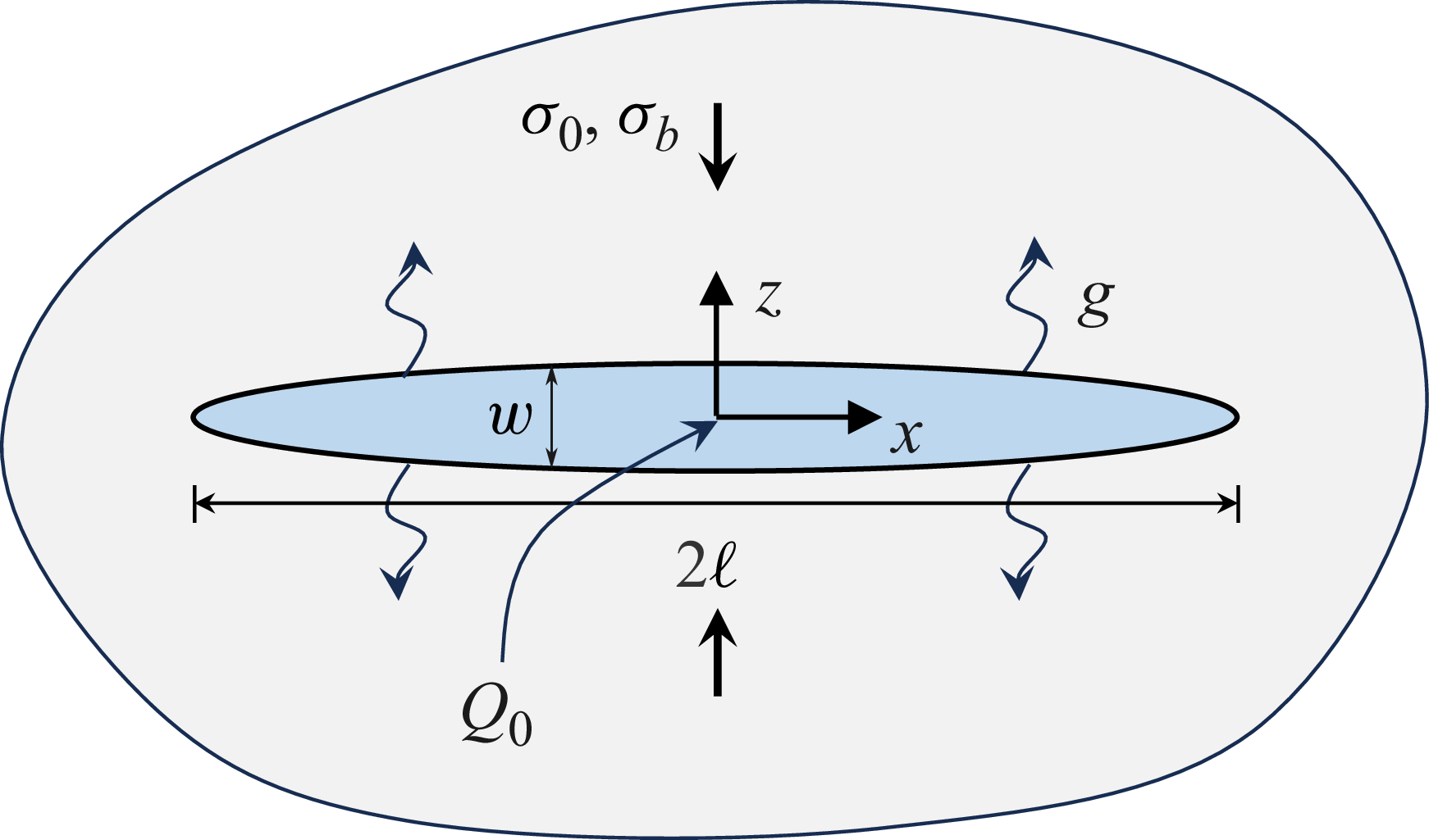

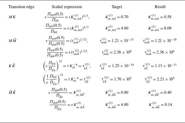
 M
 M~
 K~
 K
 ϵ=0.210
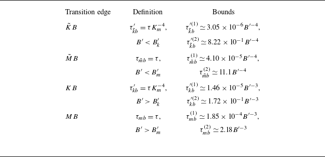
 M
 M~
 K~
 K
 B
 ϵ=0.210
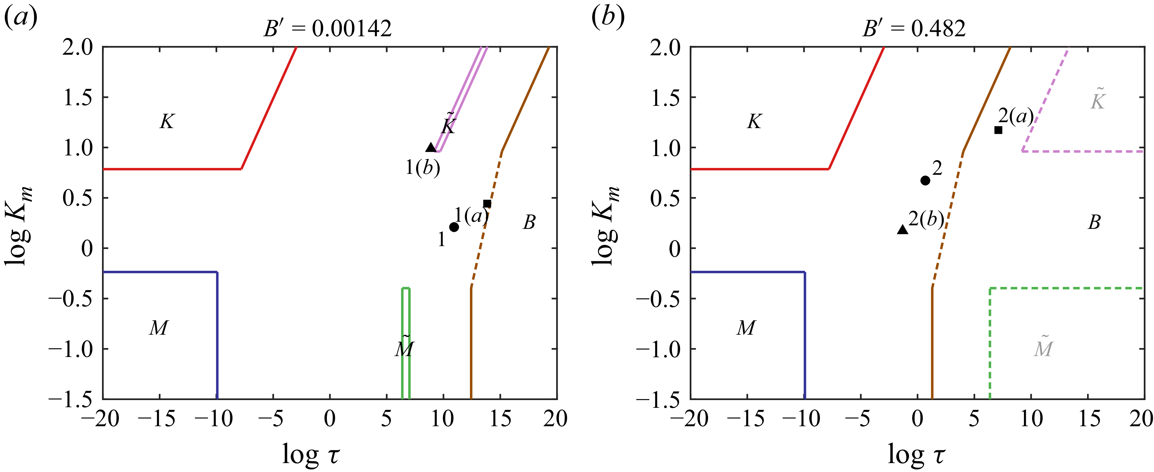
 B′
 B′>Bk′,B′>Bm′
 Bk′
 Bm′
 K
 M
 B
 B′
 K~
 M~
 B′
 M~
 K~
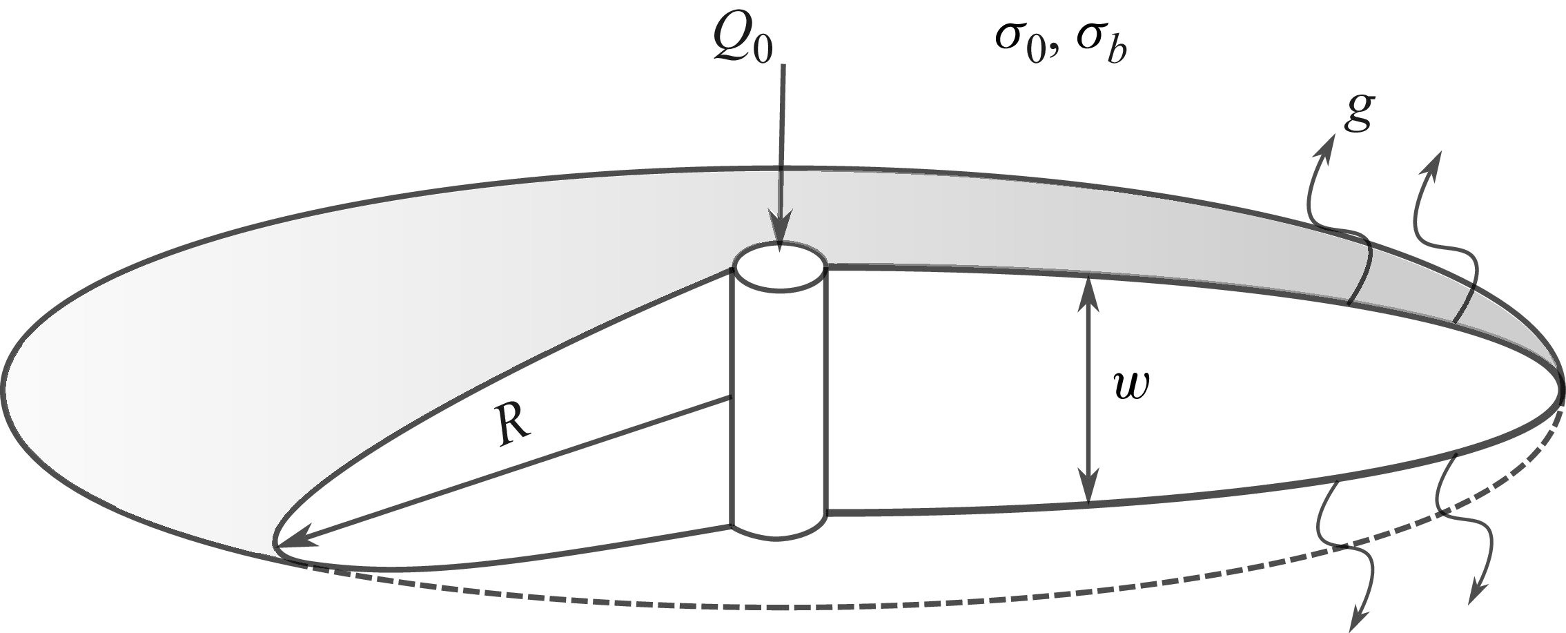

 I(ρ)
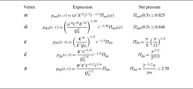
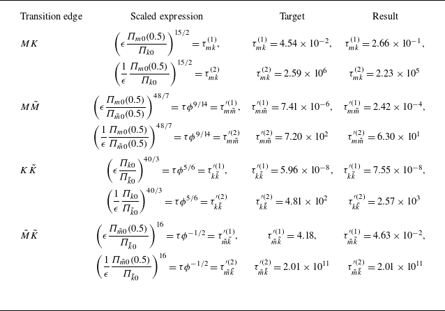
 M
 M~
 K~
 K
 ϵ=0.403
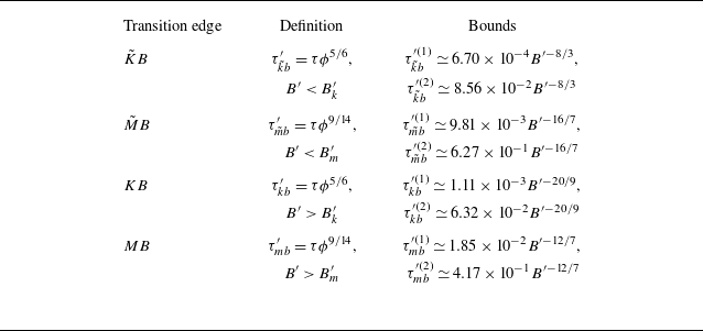
 M
 M~
 K~
 K
 B
 ϵ=0.403

 B′
 B′>Bk′,B′>Bm′
 Bk′
 Bm′
 K
 M
 B
 B′
 K~
 M~
 B′
 M~
 K~

 K~
 B
 Gk
 Gk
 K~
 B
 Gk
 Gk=B′−1τ−3/8ϕ−5/16=(B′8/3τk~b′)−3/8

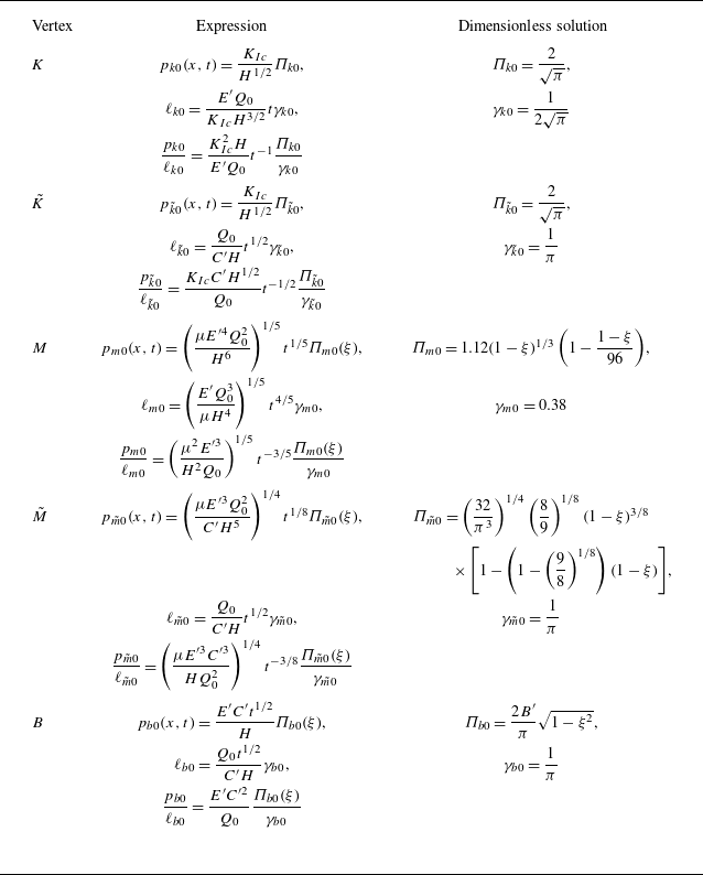
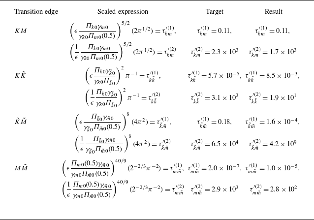
 M
 M~
 K~
 K
 ϵ=0.145
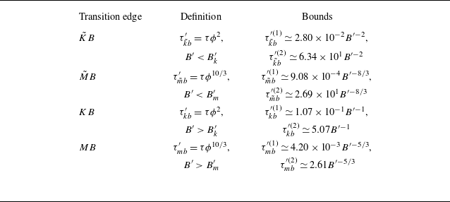
 M
 M~
 K~
 K
 B
 ϵ=0.145

 B′
 B′>Bk′,B′>Bm′
 Bk′
 Bm′
 K
 M
 B
 B′
 K~
 M~
 B′
 K~
 M~

 β
 K~B
 Gk

 K~B
 Ωk~b(ξ)
 Πk~b(ξ)
 ξ=x/ℓ(t)∈[0,1]
 ξ=0
 ξ=1
 Gk
 Ωk~0
 Πk~0
 K~
 Gk≫1
 Ωb0
 Πb0
 B
 Gk→0

 K~B
 Gk
 Ωk~b(0)
 Πk~b(0)
 ξ=0
 Ωk~0(0)
 Πk~0(0)
 K~
 Gk≫1
 Ωb0(0)
 Πb0(0)
 B
 Gk→0
 K~B
 Gk
 Gk=(πB′τ1/2ϕ)−1=(πB′2τk~b′)−1/2

 M~B
 βm~b(ξ)
 ξ=x/ℓ(t)∈[0,1]
 ξ=0
 ξ=1
 Gm
 B

 M~B
 Ωm~b(ξ)/Ωm~b(0)
 Πm~b(ξ)/Πm~b(0)
 ξ=x/ℓ(t)∈[0,1]
 ξ=0
 ξ=1
 Gm
 B

 M~B
 Gm
 Ωm~b(0)
 Πm~b(0)
 ξ=0
 Ωm~0(0)
 Πm~0(0)
 M~
 Gm≫1
 Ωb0(0)
 Πb0(0)
 B
 Gm→0
 M~B
 Gm
 Gm=1/(2π3)(B′8/3τϕ10/3)−3/2=1/(2π3)(B′8/3τm~b′)−3/2


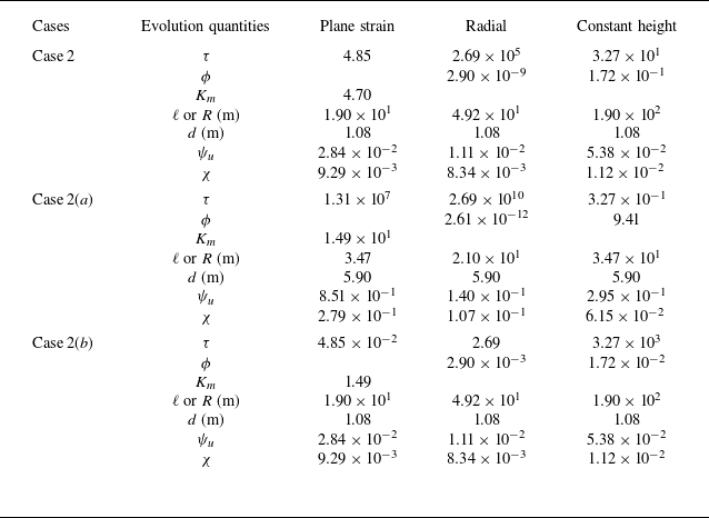

 w/⟨w⟩
 η
 β
 fq(β)


