2.1. Numerical methods

We solve the MHD equations (see Priest & Forbes Reference Priest and Forbes2000) as follows:

(2.1) \begin{align} \begin{cases} \dfrac {\partial \boldsymbol {u}}{\partial t} + \boldsymbol {u} \boldsymbol{\cdot} \boldsymbol {\nabla } \boldsymbol {u} = - \dfrac {1}{\rho } \boldsymbol {\nabla } p + \dfrac {1}{\rho } {\boldsymbol {F}}_L + \nu _k \nabla ^2 \boldsymbol {u}, \quad \boldsymbol {\nabla } \boldsymbol{\cdot} \boldsymbol {u} = 0, \\[10pt] \dfrac {\partial \boldsymbol {b}}{\partial t} = \boldsymbol {\nabla } \times (\boldsymbol {u} \times \boldsymbol {b}) + \nu _m \nabla ^2 \boldsymbol {b}, \quad \boldsymbol {\nabla } \boldsymbol{\cdot} \boldsymbol {b} = 0. \end{cases} \end{align}

In this system, $\boldsymbol {u}$ , $\boldsymbol {b}$ , $p$ , $\rho$ , $t$ , $\nu _k$ and $\nu _m$ represent the velocity, magnetic induction, pressure, mass density, time, kinematic viscosity and magnetic diffusivity, respectively. The magnetic induction $ \boldsymbol {b}$ is referred to as the magnetic field in this study, although strictly speaking, the magnetic field in vacuum is given by $ \boldsymbol {H} = \boldsymbol {b}/\mu _0$ , where $ \mu _0$ denotes the magnetic permeability of free space with a value of $ 4\unicode{x03C0} \times 10^{-7} \,\text {H}\,\text{m}^{-1}$ . The Lorentz force, ${\boldsymbol {F}}_L$ , is given by

(2.2) \begin{equation} {\boldsymbol {F}}_L \equiv \boldsymbol {j} \times \boldsymbol {b}, \end{equation}

where $\boldsymbol {j}$ is the current density, related to the magnetic induction $\boldsymbol {b}$ through Ampère’s law: $\boldsymbol {j} = \boldsymbol {\nabla } \times \boldsymbol {b}/\mu _0$ . The fluid is assumed to be incompressible, with a constant density $\rho$ . We set $\nu _k = \nu _m$ , which results in a magnetic Prandtl number, $Pr_m$ , of unity, defined as the ratio of kinematic viscosity to magnetic diffusivity (Hasimoto Reference Hasimoto1959). This choice simplifies the MHD system, facilitating both mathematical analysis and numerical simulations, particularly in qualitative studies (Linton et al. Reference Linton, Dahlburg and Antiochos2001; Kivotides Reference Kivotides2018).

We adopt the dimensionless form of (2.1), maintaining the original form of the variables for simplicity. We perform numerical simulations of MHD flows within a periodic cube $ \Omega$ of side length $L=2\unicode{x03C0}$ . The governing equation (2.1) is symmetrically reformulated using the variables $\boldsymbol {z}^{\pm } = \boldsymbol {u} \pm \boldsymbol {b}$ , as introduced by Elsasser (Reference Elsasser1950). These equations are solved with a pseudo-spectral method, following the approach of Aluie (Reference Aluie2009), which provides highly accurate computation of spatial derivatives through Fourier transformations. To reduce aliasing errors, we use the two-thirds truncation method, with a maximum wavenumber $k_{\textit{max}} \approx N/3$ . Time integration of the Fourier coefficients is carried out using a second-order Runge–Kutta scheme, with the time step chosen to maintain the Courant–Friedrichs–Lewy number below 0.5 for numerical stability. The accuracy of our MHD solver has been validated in previous studies, as cited in Hao et al. (Reference Hao, Xiong and Yang2019), Xiong & Yang (Reference Xiong and Yang2020a ) and Hao & Yang (Reference Hao and Yang2021). Details of grid convergence testing are provided in Appendix A.

Figure 1.

Schematic diagram showing the relationship between the intrinsic coordinates $(s, \varrho , \vartheta )$ and the Cartesian coordinates $(x, y, z)$ . The flux tube is outlined in light blue, with its central axis indicated in yellow-green. The cross-sectional view of the flux tube is enclosed by an orange dashed line.

We investigate the interaction between magnetic and vortical flux tubes using the methodology of Xiong & Yang (Reference Xiong and Yang2019a , Reference Xiong and Yang2020a ). The initial conditions include tubular structures derived from a continuous, differentiable curve $C: \boldsymbol {x} = \boldsymbol {c}(s)$ in three-dimensional space $\mathbb {R}^3$ , parametrised by arc length $s \in [0, L_C)$ , where $L_C$ is the length of the curve. In figure 1, the spatial coordinates $\boldsymbol {x} = (x, y, z)$ are expressed in the FS frame as $\boldsymbol {x} = \boldsymbol {c}(s) + \varrho \cos \vartheta \, \boldsymbol {N} + \varrho \sin \vartheta \, \boldsymbol {B}$ , where $\boldsymbol {T} \equiv \mathrm {d} \boldsymbol {c}/\mathrm {d} s$ is the unit tangent vector, $\boldsymbol {N} \equiv (\mathrm {d} \boldsymbol {T}/\mathrm {d} s) / (|\mathrm {d} \boldsymbol {T}/\mathrm {d} s|)$ is the unit normal vector and $\boldsymbol {B} \equiv \boldsymbol {T} \times \boldsymbol {N}$ is the unit binormal vector. Here, $\varrho = |\boldsymbol {x} - \boldsymbol {c}|$ denotes the distance between $\boldsymbol {c}(s)$ and $\boldsymbol {x}$ , and $\vartheta \in [0, 2\unicode{x03C0} )$ is the angle in the plane defined by $\boldsymbol {N}$ and $\boldsymbol {B}$ from the unit normal vector to $\boldsymbol {x}$ . This configuration positions curve $C$ as the central axis of the flux tube.

In the coordinate system $(s, \varrho , \vartheta )$ , the flux tube formulation is given by (Xiong & Yang Reference Xiong and Yang2019 a)

(2.3) \begin{equation} \boldsymbol {v}(s, \varrho , \vartheta ) = f(\varrho ) \boldsymbol {T}, \end{equation}

where the kernel function is $f(\varrho ) = \exp [-\varrho ^2/(2\sigma ^2)]/(2\unicode{x03C0} \sigma ^2)$ with $\sigma = 1/(16\sqrt {2\unicode{x03C0} })\approx 0.025$ . The flux tube’s estimated radius $ R_v$ is approximately $ 5\sigma$ , encompassing over 99.999 % of the toroidal flux. We restrict $\boldsymbol {v}$ within $ R_v$ , ensuring no self-intersections as long as $ R_v$ is smaller than the minimum curvature radius of the central axis $ C$ .

We express the initial magnetic field $\boldsymbol {b}$ in (2.1) using (2.3) as $\boldsymbol {b} = \varGamma _{m}\boldsymbol {v}$ , where $\varGamma _{m}$ denotes the circulation of the initial magnetic tube. Similarly, the vorticity field is given by $\boldsymbol {\omega } = \varGamma _k \boldsymbol {v}$ , with $\varGamma _{k}$ representing the circulation of the initial vortex tube. To obtain the velocity field $\boldsymbol {u}$ in (2.1), we solve $\boldsymbol {\omega } = \boldsymbol {\nabla } \times \boldsymbol {u}$ and $\boldsymbol {\nabla } \boldsymbol{\cdot} \boldsymbol {u} = 0$ using the Fourier transform: $ \boldsymbol {u} = \mathcal {F}^{-1} (i \boldsymbol {k} \times \hat {\boldsymbol {\omega }}/|\boldsymbol {k}|^2 ),$ where $\mathcal {F}^{-1}$ denotes the inverse Fourier transform, $\boldsymbol {k}$ is the wavenumber vector and $\hat {\boldsymbol {\omega }} = \mathcal {F}(\boldsymbol {\omega })$ is the Fourier transform of the vorticity field.

2.2. Initial configurations

We generate the initial flux tubes as a pair of interconnected tubes. The parametric equation $\boldsymbol {c}(\zeta ) = [c_x(\zeta ), c_y(\zeta ), c_z(\zeta )]$ defines the axis of the first flux tube:

(2.4) \begin{equation} \begin{cases} c_x(\zeta ) = \unicode{x03C0} +[1 + 0.5\cos (2\zeta )]\cos (\zeta ),\\ c_y(\zeta ) = \unicode{x03C0} +[1 + 0.5\cos (2\zeta )]\sin (\zeta ),\\ c_z(\zeta ) = \unicode{x03C0} -1.5-0.5\sin (2\zeta ). \end{cases} \end{equation}

The axis of the second flux tube is obtained by rotating the curve from (2.4) clockwise by $\unicode{x03C0} /2$ around the line at $(x, y) = (\unicode{x03C0} , \unicode{x03C0} )$ . As a result, the initial configuration comprises two interconnected tubes, leading to scenarios where the magnetic and vortex tubes may exhibit either right- or left-handed linkages. For simplicity, the arc length parameter for curve $C$ is not used in the above equation. Detailed formulas for computing the geometric properties of curves using a generalised parameter format are provided in Appendix A of Xiong & Yang (Reference Xiong and Yang2020a ).

Figure 2.

Isosurfaces of $|\boldsymbol {b}|$ and $|\boldsymbol {\omega }|$ for (a) $L_{m}L_{k}$ with $\theta = 0^{\,\circ}$ and (b) $L_{m}L_{k}$ with $\theta = 30^{\,\circ}$ .

We investigate various magnetic–vortex configurations, considering the presence or absence of initial vorticity and magnetic fields. Specifically, we examine systems with initial left-handed linkage $(L_{m}L_{k})$ and right-handed linkage $(R_{m}R_{k})$ for magnetic and vortex tubes, as well as pure initial magnetic flow $(L_{m}O_{k}, R_{m}O_{k})$ and purely vortical flow $(O_{m}L_{k}, O_{m}R_{k})$ , resulting in four distinct reference categories. A right-handed linkage indicates that the two interconnected closed flux tubes share the same orientation, whereas a left-handed linkage implies that they have opposite orientations. While left-handed and right-handed linkages provide a useful classification, the key determinant of their dynamics in MHD flows lies in the relative spatial arrangement and interaction of the tubes, particularly in relation to the alignment of the currents and the reconnection behaviour. We also investigate how the initial angle between the magnetic and vortex tubes influences flux tube evolution. In our notation, ‘ $R$ ’ and ‘ $L$ ’ represent flux tubes with right-handed (positive linking number +2) and left-handed linkages (negative linking number −2), respectively, while ‘ $O$ ’ indicates the absence of corresponding flux tubes. The subscripts ‘ $m$ ’ and ‘ $k$ ’ denote magnetic and kinematic vortex tubes, with ‘ $\theta$ ’ specifying their relative angle.

Figure 2 shows isosurfaces of $|\boldsymbol {\omega }|$ and $|\boldsymbol {b}|$ for various flux tube configurations, highlighting their coherent and concentrated structures. This confirms the appropriateness of the constructed flux links as initial conditions for DNS. Due to the short time scales considered, the flow structure remains approximately centred within the computational domain. The effect of periodic boundaries on the flow is minimal, given the distance-squared decay of the velocity field as described by the Biot–Savart law.

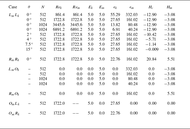
Table 1 provides the parameters and statistics for representative initial flux tubes, including the grid size $ N$ , which determines the simulation resolution. It also lists several dimensionless parameters, including the kinetic Reynolds number $ Re_{k} = \varGamma _{k} / \nu _k$ , which characterises the relative dominance of inertial forces over viscous dissipation in the kinetic field, and the magnetic Reynolds number $ Re_m = Re_k \boldsymbol{\cdot} Pr_m$ , which quantifies the relative importance of inertial versus diffusive effects in the magnetic field. Additionally, the table provides the kinetic energy $ E_{k} = \sum _k |\hat {\boldsymbol {u}}(\boldsymbol {k})|^2 / 2$ and magnetic energy $ E_{m} = \sum _k |\hat {\boldsymbol {b}}(\boldsymbol {k})|^2 / 2$ , calculated by using Fourier coefficients $ \hat {\boldsymbol {b}} = \mathcal {F}(\boldsymbol {b})$ and $ \hat {\boldsymbol {u}} = \mathcal {F}(\boldsymbol {u})$ . Additionally, it includes the kinetic dissipation rate $ \epsilon _{k} = \nu _k \sum _k (|\boldsymbol {k}| |\hat {\boldsymbol {u}}(\boldsymbol {k})|)^2$ and magnetic dissipation rate $ \epsilon _{m} = \nu _m \sum _k (|\boldsymbol {k}| |\hat {\boldsymbol {b}}(\boldsymbol {k})|)^2$ , which quantify the efficiency of the energy dissipation mechanisms in the fluid and magnetic fields. Helicity statistics are also provided, including cross-helicity $ H_c = \int _{\varOmega } \boldsymbol {u} \boldsymbol{\cdot} \boldsymbol {b} \, \mathrm {d}\varOmega$ and magnetic helicity $ H_{m} = \int _{\varOmega } \boldsymbol {a} \boldsymbol{\cdot} \boldsymbol {b} \, \mathrm {d}\varOmega$ , where $ \boldsymbol {a} = \mathcal {F}^{-1}(i \boldsymbol {k} \times \hat {\boldsymbol {b}} / |\boldsymbol {k}|^2)$ . Cross-helicity measures the correlation between the velocity and magnetic fields, while magnetic helicity provides insight into the twist and linkage of the magnetic field lines. For cases with vortex tubes, the initial vorticity flux, $\varGamma _k$ , is set to 17.228, while for cases with magnetic tubes, the initial magnetic flux, $\varGamma _m$ , is set to 1.036. This ensures that in simulations with both a magnetic tube and a vortex tube, the initial magnetic energy of the magnetic tube equals the initial kinetic energy of the vortex tube.

Table 1.

Parameters and statistics for the initial configurations of selected simulations. Here $ R$ and $ L$ denote right-handed and left-handed flux tubes with linking numbers +2 and −2, respectively. Subscripts $ m$ and $ k$ refer to magnetic and kinematic vortex tubes, with $ \theta$ specifying their angle. The initial fluxes are set to $ \varGamma _k = 17.228$ and $ \varGamma _m = 1.036$ , ensuring equal initial magnetic and kinetic energy in simulations with both types of tubes.

Figure 3.

Splitting of the magnetic tube for case $L_{m}O_k$ with $Re_m = 414.4$ at $t = 0.0175$ . Integral curves of $\boldsymbol {b}$ are coloured by the scalar field $\boldsymbol {j} \boldsymbol{\cdot} \boldsymbol {b}$ . The right-hand subfigure provides a zoomed view of the dashed box area from the left-hand subfigure.

We investigate the evolution of magnetic tubes and their interactions with vortex tubes. As shown in figure 3, a phenomenon observed is the splitting of magnetic tubes during their evolution. This study systematically explores this process by integrating theoretical analysis of the governing equations with a quantitative assessment of numerical results. Specifically, vortex dynamics analysis is used to clarify the role of vortex tubes in magnetic tube splitting.

Additionally, we observe that, in our numerical simulations involving both magnetic and vortex tubes, the Lorentz force is substantially larger than the inertial force. This relationship can be characterised by the interaction parameter $ N_{I} = \varGamma _m^2 / [\rho \mu _0 Re_k \nu _k\nu _m (R_v)^2 ]=(\varGamma _m^2Re_k)/\rho \mu _0 (\varGamma _k R_v)^2$ , which quantifies the balance between Lorentz and inertial forces in the system (Kivotides Reference Kivotides2018, Reference Kivotides2019). In the simulations presented herein, $ N_I \gg 1$ , and in this regime, the morphologies of the vorticity and magnetic field structures exhibit notable similarity. This phenomenon is further explored in the following sections and aligns with the observations of Kivotides (Reference Kivotides2018).

3.1. The FS frame fields

To facilitate the analysis of dynamic flow fields, we extend the FS frame throughout the flux tube domain. This FS frame is defined where the magnetic field and the curvature of the magnetic lines are both non-zero, although it is important to note that inflexion points may exist in realistic scenarios. Specifically, we define a FS coordinate system at each point along the magnetic field lines, establishing a unit frame field $[\boldsymbol {T}(\boldsymbol {x}), \boldsymbol {N}(\boldsymbol {x}), \boldsymbol {B}(\boldsymbol {x})]$ at locations where the magnetic field is non-zero, as depicted in figure 4. At each point $\boldsymbol {c}$ along these magnetic lines, the vectors $[\boldsymbol {T}(\boldsymbol {c}), \boldsymbol {N}(\boldsymbol {c}), \boldsymbol {B}(\boldsymbol {c})]$ follow the FS formulas:

(3.1) \begin{equation} {\boldsymbol {T}} \boldsymbol{\cdot} \boldsymbol \nabla {\boldsymbol {T}} = \kappa {\boldsymbol {N}},\quad {\boldsymbol {T}} \boldsymbol{\cdot} \boldsymbol \nabla {\boldsymbol {N}} = -\kappa {\boldsymbol {T}} + \tau {\boldsymbol {B}},\quad {\boldsymbol {T}} \boldsymbol{\cdot} \boldsymbol \nabla {\boldsymbol {B}} =-\tau {\boldsymbol {N}}. \end{equation}

Here, $\kappa$ and $\tau$ represent the curvature and torsion of the curve, respectively.

Figure 4.

Frenet–Serret frames generated by magnetic field lines. The unit tangent, normal and binormal vectors are represented by black, blue and red arrows, respectively.

Let $\boldsymbol {T}$ , $\boldsymbol {N}$ and $\boldsymbol {B}$ be column vectors that form an orthogonal matrix $\mathcal {O} = [\boldsymbol {T}, \boldsymbol {N}, \boldsymbol {B}]$ . Utilising the properties of the matrix trace, for any matrix $\boldsymbol {A}$ , we have

(3.2) \begin{equation} \textrm {Tr}(\boldsymbol A)= \textrm {Tr}(\mathcal {O}^{-1}\boldsymbol A \mathcal {O})= \textrm {Tr}(\mathcal {O}^{T}\boldsymbol A \mathcal {O})= \boldsymbol T^T\boldsymbol A \boldsymbol T + \boldsymbol N^T\boldsymbol A \boldsymbol N + \boldsymbol B^T\boldsymbol A \boldsymbol B. \end{equation}

Since $\boldsymbol {T}$ , $\boldsymbol {N}$ and $\boldsymbol {B}$ are unit vectors, and applying (3.2) and $\boldsymbol {\nabla } \boldsymbol{\cdot} \boldsymbol {A} = \text {Tr}(\boldsymbol {\nabla } \boldsymbol {A})$ , we obtain

(3.3) \begin{equation} \begin{cases} \boldsymbol \nabla \boldsymbol{\cdot} \boldsymbol T = \boldsymbol T \boldsymbol{\cdot} \boldsymbol \nabla \boldsymbol T \boldsymbol{\cdot} \boldsymbol T + \boldsymbol N \boldsymbol{\cdot} \boldsymbol \nabla \boldsymbol T \boldsymbol{\cdot} \boldsymbol N + \boldsymbol B \boldsymbol{\cdot} \boldsymbol \nabla \boldsymbol T \boldsymbol{\cdot} \boldsymbol B= \boldsymbol N \boldsymbol{\cdot} \boldsymbol \nabla \boldsymbol T \boldsymbol{\cdot} \boldsymbol N + \boldsymbol B \boldsymbol{\cdot} \boldsymbol \nabla \boldsymbol T \boldsymbol{\cdot} \boldsymbol B , \\ \boldsymbol \nabla \boldsymbol{\cdot} \boldsymbol N = \boldsymbol T \boldsymbol{\cdot} \boldsymbol \nabla \boldsymbol N \boldsymbol{\cdot} \boldsymbol T + \boldsymbol N \boldsymbol{\cdot} \boldsymbol \nabla \boldsymbol N \boldsymbol{\cdot} \boldsymbol N + \boldsymbol B \boldsymbol{\cdot} \boldsymbol \nabla \boldsymbol N \boldsymbol{\cdot} \boldsymbol B =\boldsymbol T \boldsymbol{\cdot} \boldsymbol \nabla \boldsymbol N \boldsymbol{\cdot} \boldsymbol T + \boldsymbol B \boldsymbol{\cdot} \boldsymbol \nabla \boldsymbol N \boldsymbol{\cdot} \boldsymbol B, \\ \boldsymbol \nabla \boldsymbol{\cdot} \boldsymbol B =\boldsymbol T \boldsymbol{\cdot} \boldsymbol \nabla \boldsymbol B \boldsymbol{\cdot} \boldsymbol T + \boldsymbol N \boldsymbol{\cdot} \boldsymbol \nabla \boldsymbol B \boldsymbol{\cdot} \boldsymbol N + \boldsymbol B \boldsymbol{\cdot} \boldsymbol \nabla \boldsymbol B \boldsymbol{\cdot} \boldsymbol B =\boldsymbol T \boldsymbol{\cdot} \boldsymbol \nabla \boldsymbol B \boldsymbol{\cdot} \boldsymbol T +\boldsymbol N \boldsymbol{\cdot} \boldsymbol \nabla \boldsymbol B \boldsymbol{\cdot} \boldsymbol N. \\ \end{cases} \end{equation}

Additionally, for three-dimensional vectors $\boldsymbol f$ and $\boldsymbol g$ , using

(3.4) \begin{equation} \boldsymbol \nabla \times (\boldsymbol f \times \boldsymbol g) = -(\boldsymbol \nabla \boldsymbol{\cdot} \boldsymbol f)\boldsymbol g +(\boldsymbol \nabla \boldsymbol{\cdot} \boldsymbol g)\boldsymbol f +\boldsymbol g \boldsymbol{\cdot} \boldsymbol \nabla \boldsymbol f - \boldsymbol f \boldsymbol{\cdot} \boldsymbol \nabla \boldsymbol g \end{equation}

and (3.3), we obtain

(3.5) \begin{equation} \begin{aligned} \boldsymbol \nabla \times \boldsymbol T &= \boldsymbol \nabla \times (\boldsymbol N \times \boldsymbol B) = -(\boldsymbol \nabla \boldsymbol{\cdot} \boldsymbol N)\boldsymbol B +(\boldsymbol \nabla \boldsymbol{\cdot} \boldsymbol B)\boldsymbol N +\boldsymbol B \boldsymbol{\cdot} \boldsymbol \nabla \boldsymbol N - \boldsymbol N \boldsymbol{\cdot} \boldsymbol \nabla \boldsymbol B\\ &= ( \boldsymbol N \boldsymbol{\cdot} \boldsymbol \nabla \boldsymbol T \boldsymbol{\cdot} \boldsymbol B - \boldsymbol B \boldsymbol{\cdot} \boldsymbol \nabla \boldsymbol T \boldsymbol{\cdot} \boldsymbol N) \boldsymbol T +(\boldsymbol \nabla \boldsymbol{\cdot} \boldsymbol B+\boldsymbol N \boldsymbol{\cdot} \boldsymbol \nabla \boldsymbol N \boldsymbol{\cdot} \boldsymbol B)\boldsymbol N\\ & \quad +(\boldsymbol B \boldsymbol{\cdot} \boldsymbol \nabla \boldsymbol N \boldsymbol{\cdot} \boldsymbol B-\boldsymbol \nabla \boldsymbol{\cdot} \boldsymbol N)\boldsymbol B \\ &= ( \boldsymbol N \boldsymbol{\cdot} \boldsymbol \nabla \boldsymbol T \boldsymbol{\cdot} \boldsymbol B - \boldsymbol B \boldsymbol{\cdot} \boldsymbol \nabla \boldsymbol T \boldsymbol{\cdot} \boldsymbol N) \boldsymbol T +(\boldsymbol T \boldsymbol{\cdot} \boldsymbol \nabla \boldsymbol B \boldsymbol{\cdot} \boldsymbol T)\boldsymbol N -(\boldsymbol T \boldsymbol{\cdot} \boldsymbol \nabla \boldsymbol N \boldsymbol{\cdot} \boldsymbol T)\boldsymbol B. \end{aligned} \end{equation}

Similarly, we have

(3.6) \begin{equation} \begin{cases} \boldsymbol \nabla \times \boldsymbol N = -(\boldsymbol N \boldsymbol{\cdot} \boldsymbol \nabla \boldsymbol B \boldsymbol{\cdot} \boldsymbol N)\boldsymbol T+ ( \boldsymbol B \boldsymbol{\cdot} \boldsymbol \nabla \boldsymbol N \boldsymbol{\cdot} \boldsymbol T - \boldsymbol T \boldsymbol{\cdot} \boldsymbol \nabla \boldsymbol N \boldsymbol{\cdot} \boldsymbol B) \boldsymbol N +(\boldsymbol N \boldsymbol{\cdot} \boldsymbol \nabla \boldsymbol T \boldsymbol{\cdot} \boldsymbol N)\boldsymbol B ,\\ \boldsymbol \nabla \times \boldsymbol B = (\boldsymbol B \boldsymbol{\cdot} \boldsymbol \nabla \boldsymbol N \boldsymbol{\cdot} \boldsymbol B)\boldsymbol T -(\boldsymbol B \boldsymbol{\cdot} \boldsymbol \nabla \boldsymbol T \boldsymbol{\cdot} \boldsymbol B)\boldsymbol N + ( \boldsymbol T \boldsymbol{\cdot} \boldsymbol \nabla \boldsymbol B \boldsymbol{\cdot} \boldsymbol N - \boldsymbol N \boldsymbol{\cdot} \boldsymbol \nabla \boldsymbol B \boldsymbol{\cdot} \boldsymbol T) \boldsymbol B . \end{cases} \end{equation}

Substituting (3.1) into (3.3), (3.5) and (3.6) yields

(3.7) \begin{equation} \begin{cases} \boldsymbol \nabla \boldsymbol{\cdot} \boldsymbol T =\boldsymbol N \boldsymbol{\cdot} \boldsymbol \nabla \boldsymbol T \boldsymbol{\cdot} \boldsymbol N + \boldsymbol B \boldsymbol{\cdot} \boldsymbol \nabla \boldsymbol T \boldsymbol{\cdot} \boldsymbol B , \\ \boldsymbol \nabla \boldsymbol{\cdot} \boldsymbol N =-\kappa + \boldsymbol B \boldsymbol{\cdot} \boldsymbol \nabla \boldsymbol N \boldsymbol{\cdot} \boldsymbol B, \\ \boldsymbol \nabla \boldsymbol{\cdot} \boldsymbol B =\boldsymbol N \boldsymbol{\cdot} \boldsymbol \nabla \boldsymbol B \boldsymbol{\cdot} \boldsymbol N\\ \end{cases} \end{equation}

and

(3.8) \begin{equation} \begin{cases} \boldsymbol \nabla \times \boldsymbol T = ( \boldsymbol N \boldsymbol{\cdot} \boldsymbol \nabla \boldsymbol T \boldsymbol{\cdot} \boldsymbol B - \boldsymbol B \boldsymbol{\cdot} \boldsymbol \nabla \boldsymbol T \boldsymbol{\cdot} \boldsymbol N) \boldsymbol T +\kappa \boldsymbol B , \\ \boldsymbol \nabla \times \boldsymbol N =-(\boldsymbol N \boldsymbol{\cdot} \boldsymbol \nabla \boldsymbol B \boldsymbol{\cdot} \boldsymbol N)\boldsymbol T-( \tau + \boldsymbol B \boldsymbol{\cdot} \boldsymbol \nabla \boldsymbol T \boldsymbol{\cdot} \boldsymbol N ) \boldsymbol N +(\boldsymbol N \boldsymbol{\cdot} \boldsymbol \nabla \boldsymbol T \boldsymbol{\cdot} \boldsymbol N)\boldsymbol B, \\ \boldsymbol \nabla \times \boldsymbol B = (\boldsymbol B \boldsymbol{\cdot} \boldsymbol \nabla \boldsymbol N \boldsymbol{\cdot} \boldsymbol B)\boldsymbol T -(\boldsymbol B \boldsymbol{\cdot} \boldsymbol \nabla \boldsymbol T \boldsymbol{\cdot} \boldsymbol B)\boldsymbol N + (\boldsymbol N \boldsymbol{\cdot} \boldsymbol \nabla \boldsymbol T\boldsymbol{\cdot} \boldsymbol B- \tau ) \boldsymbol B. \\ \end{cases} \end{equation}

3.2. Lorentz force in the FS frame field

By aligning the FS frame with the magnetic field lines, the tangent vector $\boldsymbol {T}$ is made parallel to the magnetic field. Within this coordinate system, we investigate the Lorentz force acting on the magnetic tube and elucidate the mechanism underlying its splitting.

Using the FS frame field, the Lorentz force, as expressed in (2.2), can be represented as

(3.9) \begin{equation} {\boldsymbol {F}}_L =-\boldsymbol{\nabla} {\boldsymbol {b}} \boldsymbol{\cdot} {\boldsymbol {b}} + {\boldsymbol {b}} \boldsymbol{\cdot} \boldsymbol{\nabla} {\boldsymbol {b}} = -\tfrac {1}{2}\boldsymbol{\nabla} b^2 + b({\boldsymbol {T}} \boldsymbol{\cdot} \boldsymbol{\nabla} b){\boldsymbol {T}} +\kappa b^2 {\boldsymbol {N}}. \end{equation}

Here, $\kappa$ denotes the curvature of the magnetic lines. We remark that $(\boldsymbol {T}, \boldsymbol {B}, \boldsymbol {N})$ and $\kappa$ are computed for each magnetic field line considered as a parametrised curve. Consequently, these quantities define fields that are distributed throughout the flux tube. In Ricca (Reference Ricca2005), the Lorentz force is derived through the geometry of magnetic field lines, with a focus on their curvature and torsion. The study emphasises how the curvature of the magnetic field lines contributes to the instability of flux tubes, particularly when inflection points are present. Similarly, (3.9) provides a geometrical interpretation of the forces acting on the flux tubes, highlighting the role of curvature in destabilising the magnetic structures.

Given the divergence-free property of the vector field $\boldsymbol {b}$ in (2.1), we arrive at the following relation:

(3.10) \begin{equation} b \boldsymbol \nabla \boldsymbol{\cdot} {\boldsymbol {T}} + {\boldsymbol {T}} \boldsymbol{\cdot} \boldsymbol \nabla b=0. \end{equation}

Substituting (3.10) into (3.9) yields

(3.11) \begin{equation} {\boldsymbol {F}}_L =-\tfrac {1}{2}\boldsymbol \nabla b^2 + b^2\left [-(\boldsymbol \nabla \boldsymbol{\cdot} {\boldsymbol {T}}) {\boldsymbol {T}}+\kappa {\boldsymbol {N}} \right ]. \end{equation}

We focus on the influence of the Lorentz force on vorticity evolution to elucidate the vortex dynamics induced by MHD effects. To evaluate the vorticity evolution, we apply the curl operator to the first equation in (2.1), yielding

(3.12) \begin{equation} \frac {{\mathrm{D}} \omega }{{\mathrm{D}}t}=\omega \boldsymbol{\cdot} \boldsymbol \nabla {\boldsymbol {u}}+\nu _k\nabla ^2 \omega +\boldsymbol \nabla \times {\boldsymbol {F}}_L. \end{equation}

Here, $ {\mathrm{D}}/{\mathrm{D}}t= \partial /\partial t + \boldsymbol {u} \boldsymbol{\cdot} \boldsymbol {\nabla }$ represents the material derivative. This Lagrangian equation describes the dynamics of vorticity during the shearing process. The vorticity generation arises from the curl of the Lorentz force, which is induced by the magnetic field.

Taking the curl of (3.11) yields

(3.13) \begin{equation} \boldsymbol \nabla \times {\boldsymbol {F}}_L= \boldsymbol \nabla \times \left \{b^2\left [-(\boldsymbol \nabla \boldsymbol{\cdot} {\boldsymbol {T}}) {\boldsymbol {T}}+\kappa {\boldsymbol {N}} \right ]\right \}. \end{equation}

Equation (3.13) reveals that the curl of the Lorentz force splits into two components: $\boldsymbol {\nabla } \times {\boldsymbol {F}}_L = \boldsymbol {\omega }^{g} + \boldsymbol {\omega }^{b}$ . The first component, $\boldsymbol {\omega }^{g}$ , is defined as

(3.14) \begin{equation} \boldsymbol {\omega }^{g} = b^2 \boldsymbol \nabla \times \left [-(\boldsymbol \nabla \boldsymbol{\cdot} {\boldsymbol {T}}) {\boldsymbol {T}}+\kappa {\boldsymbol {N}} \right ] \end{equation}

and is sensitive to the geometric configuration of the magnetic field lines. On the other hand, the second component, $\boldsymbol {\omega }^{b}$ , is given by

(3.15) \begin{equation} \boldsymbol \omega ^{b}=(\boldsymbol \nabla b^2) \times \left [-(\boldsymbol \nabla \boldsymbol{\cdot} {\boldsymbol {T}}) {\boldsymbol {T}}+\kappa {\boldsymbol {N}} \right ] \end{equation}

and is sensitive to variations in magnetic intensity.

The splitting of the magnetic tube is noticeable in the early stages of its evolution. During this phase, the Lorentz force is largely influenced by the initial magnetic field configuration. Accordingly, we examine the initial condition described by (2.3), where the helicity of the vector field is influenced by the writhe of the tube axis (Xiong & Yang Reference Xiong and Yang2019a ). At this stage, the magnetic field lines have a relatively simple structure, which allows for a more straightforward decomposition of the Lorentz force.

Within the flux tube of radius $R_v$ , the flux lines corresponding to (2.3) are parallel, thus satisfying

(3.16) \begin{equation} \boldsymbol N \boldsymbol{\cdot} \boldsymbol \nabla \boldsymbol T = \boldsymbol B \boldsymbol{\cdot} \boldsymbol \nabla \boldsymbol T = \boldsymbol 0. \end{equation}

Since $\boldsymbol \nabla \boldsymbol T$ is a second-order tensor, its contraction with vectors yields a vector. From (3.1) and (3.16), we also derive the following system of equations:

(3.17) \begin{equation} \boldsymbol B \boldsymbol{\cdot} \boldsymbol \nabla \left (\boldsymbol T \boldsymbol{\cdot} \boldsymbol \nabla \boldsymbol T\right ) =\boldsymbol 0,\quad\boldsymbol N \boldsymbol{\cdot} \boldsymbol \nabla \left (\boldsymbol T \boldsymbol{\cdot} \boldsymbol \nabla \boldsymbol T\right ) =\kappa ^2 \boldsymbol N, \end{equation}

which leads to

(3.18) \begin{equation} \boldsymbol B \boldsymbol{\cdot} \boldsymbol \nabla \boldsymbol N \boldsymbol{\cdot} \boldsymbol B= \boldsymbol B \boldsymbol{\cdot} \boldsymbol \nabla \left (\frac {\boldsymbol T \boldsymbol{\cdot} \boldsymbol \nabla \boldsymbol T }{\kappa } \right ) \boldsymbol{\cdot} \boldsymbol B=0,\quad \boldsymbol N \boldsymbol{\cdot} \boldsymbol \nabla \boldsymbol B \boldsymbol{\cdot} \boldsymbol N= -\boldsymbol N \boldsymbol{\cdot} \boldsymbol \nabla \left (\frac {\boldsymbol T \boldsymbol{\cdot} \boldsymbol \nabla \boldsymbol T }{\kappa } \right ) \boldsymbol{\cdot} \boldsymbol B=0. \end{equation}

Using (3.16) and (3.18), the expressions represented by (3.7) and (3.8) can be simplified to the following results:

(3.19) \begin{equation} \boldsymbol \nabla \boldsymbol{\cdot} \boldsymbol T = 0,\quad \boldsymbol \nabla \boldsymbol{\cdot} \boldsymbol N =-\kappa , \quad \boldsymbol \nabla \boldsymbol{\cdot} \boldsymbol B =0 \end{equation}

and

(3.20) \begin{equation} \boldsymbol \nabla \times \boldsymbol T = \kappa \boldsymbol B , \quad \boldsymbol \nabla \times \boldsymbol N =- \tau \boldsymbol N, \quad \boldsymbol \nabla \times \boldsymbol B =- \tau \boldsymbol B. \end{equation}

Here, $\kappa$ and $\tau$ denote the curvature and torsion of the curve, respectively.

Figure 5.

(a) Isosurface of $|{\boldsymbol {b}}|$ for the initial flux tube from (2.3), colour-coded by $-{\boldsymbol {B}} \boldsymbol{\cdot} \boldsymbol \nabla (b^2 \kappa )$ . Black lines are integrals of $-{\boldsymbol {B}} \boldsymbol{\cdot} \boldsymbol \nabla (b^2 \kappa ) {\boldsymbol {T}}$ . (b) Zoomed view of the flux tube near the region marked by the black square in (a), with black lines indicating the integral curves of $\boldsymbol {\nabla } \times (\boldsymbol {\nabla } \times {\boldsymbol {F}}_L)$ , illustrating the dipole structure induced by the magnetic field.

Figure 6.

(a) Initial geometry of a single connected magnetic tube in the linked configuration $L_{m}O_{k}$ . The grey semi-transparent tube shows the isosurface of magnetic field strength, with curvature indicated by the colour-coded centreline. The vectors along the centreline represent the binormal vector $\boldsymbol {B}$ , with their length and colour corresponding to the torsion $\tau$ . Positions A, B and C correspond to the locations of maximum curvature, minimum curvature and maximum torsion, respectively. (b) Isosurface of $|\boldsymbol {b}| = 50$ at $t = 0.01$ , with red arrows indicating the direction of the binormal vector. Zoomed views of (b) are provided in (c) near A, (d) near B and (e) near C. The distance between the split tubes is denoted by $d$ .

We remark that both $\boldsymbol {B}$ and $\boldsymbol {N}$ in (3.20) are Beltrami vector fields (see Reed Reference Reed1995), which can be linked to chaotic magnetic lines in MHD flows (see Smiet et al. Reference Smiet, Candelaresi, Thompson, Swearngin, Dalhuisen and Bouwmeester2015). The analysis method used for this local frame field is similar to the approach of Gibbon et al. (Reference Gibbon, Holm, Kerr and Roulstone2006) for quaternions, as both involve differentiating the local frame to capture the fluid’s key dynamics.

Using (3.19) and (3.20), we simplify (3.13) to

(3.21) \begin{equation} \boldsymbol \nabla \times {\boldsymbol {F}}_L=\boldsymbol \nabla \times \left(b^2\kappa {\boldsymbol {N}}\right)=- \left[\boldsymbol B \boldsymbol{\cdot} \boldsymbol \nabla \left(b^2 \kappa \right)\right] \boldsymbol T - b^2 \kappa \tau \boldsymbol N + b^2 (\boldsymbol T \boldsymbol{\cdot} \boldsymbol \nabla \kappa ) {\boldsymbol {B}}. \end{equation}

In this study, dynamical interactions are observed within the elongated tubular structures where

(3.22) \begin{equation} \left|\left[\boldsymbol B \boldsymbol{\cdot} \boldsymbol \nabla \left(b^2 \kappa \right)\right] \boldsymbol T\right| \gg \left|b^2 \kappa \tau \boldsymbol N\right|\,\,\textrm {and}\,\, \left|\left[\boldsymbol B \boldsymbol{\cdot} \boldsymbol \nabla \left(b^2 \kappa \right)\right] \boldsymbol T\right| \gg \left| b^2 (\boldsymbol T \boldsymbol{\cdot} \boldsymbol \nabla \kappa ) {\boldsymbol {B}}\right|. \end{equation}

This dominance arises due to the typically large gradient of $ b$ . Consequently, the first term in (3.21) is the primary contributor to the evolution of the magnetic tube.

Figure 5 shows the distribution of the magnitude of the first term from (3.21) along the initial magnetic tube described by (2.3). The term $[- {\boldsymbol {B}} \boldsymbol{\cdot} \boldsymbol {\nabla } (b^2 \kappa )] {\boldsymbol {T}}$ dominates over the other terms, creating a vortex source along the tube’s axis. Additionally, this term varies in sign along the binormal direction, indicating opposing vortex sources, as illustrated in figures 5(a) and 5(b). The other terms, $|b^2 \kappa \tau \boldsymbol N|$ and $|b^2 ({\boldsymbol {T}} \boldsymbol{\cdot} \boldsymbol \nabla \kappa )\boldsymbol B|$ , reach their maxima where $\kappa \tau$ and $({\boldsymbol {T}} \boldsymbol{\cdot} \boldsymbol \nabla \kappa )$ are largest, respectively. However, these terms are generally much smaller than the first term (figures not shown).

Figure 6(a) shows the initial distributions of curvature $\kappa$ , torsion $\tau$ and binormal vector $\boldsymbol {B}$ along the central line of one of the flux tubes in the $L_{m}O_{k}$ case. The variations in curvature and torsion are relatively small. Positions A, B and C correspond to the locations of maximum curvature, minimum curvature and maximum torsion, respectively. Figure 6(b) indicates that the splitting direction is closely aligned with the binormal direction of the initial magnetic tube. At position A, where curvature is greater than that at B, the distance between the split tubes is larger, as shown in figures 6(c) and 6(d). It is observed that greater curvature intensifies the formation of vortex pairs, thereby accelerating the splitting of the tube. Figure 6(e) illustrates that twisting can hinder the magnetic tube’s splitting, in agreement with Xiong & Yang (Reference Xiong and Yang2020b ).

We remark that each term in (3.21) involves curvature. For instance, in a one-dimensional cylindrical magnetic tube with a flux distribution described by (2.3), where $\kappa = 0$ , the curl of the Lorentz force, $\boldsymbol \nabla \times {\boldsymbol {F}}_L$ , equals zero. Consequently, such a cylindrical magnetic tube does not act as a source of vorticity and thus does not lead to the splitting of the magnetic tube.

Figure 7.

Isosurfaces of $|\boldsymbol {b}|$ for a flow with an initially toroidal magnetic tube of constant curvature $\kappa = 4$ for (a) $|\boldsymbol {b}| = 50$ at $t = 0$ and (b) $|\boldsymbol {b}| = 20$ at $t = 0.005$ . The isosurfaces are colour-coded by ${\boldsymbol {T}} \boldsymbol{\cdot} (\boldsymbol \nabla \times {\boldsymbol {F}}_L)$ , with streamlines integrated along $\boldsymbol {u}$ in (b).

If the initial magnetic tube possesses curvature, even if it remains constant along the magnetic field lines, tube splitting can still occur. For example, for a magnetic tube with its central line lying in a plane and under the conditions $\tau = 0$ and $\boldsymbol {T} \boldsymbol{\cdot} \boldsymbol {\nabla } \kappa = 0$ , the expression of (3.21) simplifies to $\boldsymbol \nabla \times {\boldsymbol {F}}_L = -(\kappa \boldsymbol {B} \boldsymbol{\cdot} \boldsymbol {\nabla } b^2) \boldsymbol {T}$ . This indicates that the vorticity source is aligned parallel to the magnetic tube.

Figures 7(a) and 7(b) illustrate the evolution of the $|{\boldsymbol {b}}|$ isosurface, coloured by $\boldsymbol {T} \boldsymbol{\cdot} (\boldsymbol \nabla \times {\boldsymbol {F}}_L)$ , at $t = 0$ and $0.005$ . The initial toroidal magnetic tube generates opposing vortex sources in the positive and negative $z$ directions, causing them to move apart. As they separate, the split tubes continue to produce opposing vortex sources, which may lead to sustained tube splitting. In this magnetic tube configuration, we further confirm that a larger curvature $\kappa$ leads to a greater separation between the split tubes, driven by the stronger vortex pairs induced by $-(\kappa \boldsymbol {B} \boldsymbol{\cdot} \boldsymbol {\nabla } b^2) \boldsymbol {T}$ .

3.3. Material properties of integral curves in vector fields

A key feature observed during the evolution is that the magnetic and vortex tubes exhibit quasi-Lagrangian characteristics, approximately following the fluid velocity field while interacting with each other. This behaviour leads to the vortex tubes induced by the magnetic field reflecting the motion of the magnetic tubes in the early stages, including similar splitting phenomena. We explore this behaviour through an analysis of the governing equations for the vorticity and magnetic fields.

Specifically, despite the effects of magnetic interactions, the flow field associated with the evolution of strong magnetic tubes closely follows the Helmholtz (Reference Helmholtz1858) vorticity conservation theorem and the Alfvén (Reference Alfvén1943) frozen-in field theorem. The near-preservation of these conservation laws underscores the robustness of Lagrangian dynamics, even under strong magnetic influences.

To analyse the temporal evolution of the vorticity field, we neglect viscosity and apply the approximation

(3.23) \begin{equation} \boldsymbol \nabla \times {\boldsymbol {F}}_L\approx -\left[{\boldsymbol {B}}\boldsymbol{\cdot} \boldsymbol \nabla \left(b^2\kappa \right)\right]{\boldsymbol {T}} \end{equation}

to (3.21). Consequently, (3.12) simplifies to

(3.24) \begin{equation} \frac {{\mathrm{D}} \omega }{{\mathrm{D}}t}\approx \omega \boldsymbol{\cdot} \boldsymbol \nabla {\boldsymbol {u}}-\left[{\boldsymbol {B}}\boldsymbol{\cdot} \boldsymbol \nabla \left(b^2\kappa \right)\right]{\boldsymbol {T}}. \end{equation}

For the temporal evolution of the magnetic field, we consider the second equation in (2.1). By substituting $ \boldsymbol {\nabla } \times (\boldsymbol {u} \times \boldsymbol {b})$ with $ (\boldsymbol {b} \boldsymbol{\cdot} \boldsymbol {\nabla } \boldsymbol {u} - \boldsymbol {u} \boldsymbol{\cdot} \boldsymbol {\nabla } \boldsymbol {b})$ and neglecting magnetic viscous dissipation, the equation simplifies to

(3.25) \begin{equation} \frac {{\mathrm{D}} \boldsymbol {b}}{{\mathrm{D}}t} \approx \boldsymbol {b} \boldsymbol{\cdot} \boldsymbol {\nabla } \boldsymbol {u}. \end{equation}

Thus, both the magnetic equation (3.25) and the vorticity equation (3.24) can be approximately reduced to a unified form:

(3.26) \begin{equation} \frac {{\mathrm{D}}{\boldsymbol {L}}}{{\mathrm{D}}t}={\boldsymbol {L}}\boldsymbol{\cdot} \boldsymbol \nabla {\boldsymbol {u}}+\lambda {\boldsymbol {L}}, \end{equation}

where $\lambda = 0$ for ${\boldsymbol {L}} = \boldsymbol {b}$ and $\lambda = -[\boldsymbol {B} \boldsymbol{\cdot} \boldsymbol \nabla (b^2 \kappa )] / |\boldsymbol {\omega }|$ for ${\boldsymbol {L}} = \boldsymbol {\omega }$ . We present Corollary 1, which shows that the integral curves of $\boldsymbol {L}$ in (3.26) correspond to material curves.

Proof. Assume that $\phi (\boldsymbol {x}, t)$ is a scalar field that evolves over time, with its isosurfaces representing level sets of constant $\phi$ . Initially, these isosurfaces are aligned with the vector field $\boldsymbol {L}$ , implying that $\boldsymbol {L}$ lies tangentially along the isosurfaces, i.e.

(3.27) \begin{equation} \boldsymbol L \boldsymbol{\cdot} \boldsymbol \nabla \phi |_{t=0} = 0, \end{equation}

and that the isosurfaces of $\phi$ are material surfaces, satisfying ${\mathrm{D}}\phi /{\mathrm{D}} t =0$ , we have

(3.28) \begin{equation} \frac {{\mathrm{D}} (\boldsymbol L \boldsymbol{\cdot} \boldsymbol \nabla \phi )}{{\mathrm{D}} t} = \frac {{\mathrm{D}} \boldsymbol L}{{\mathrm{D}} t} \boldsymbol{\cdot} \boldsymbol \nabla \phi + \boldsymbol L \boldsymbol{\cdot} \frac {{\mathrm{D}} (\boldsymbol \nabla \phi )}{{\mathrm{D}} t} =\frac {{\mathrm{D}} \boldsymbol L}{{\mathrm{D}} t} \boldsymbol{\cdot} \boldsymbol \nabla \phi - \boldsymbol L \boldsymbol{\cdot} \boldsymbol \nabla \boldsymbol u \boldsymbol{\cdot} \boldsymbol \nabla \phi . \end{equation}

Substituting (3.26) into (3.28), we get

(3.29) \begin{equation} \frac {{\mathrm{D}} (\boldsymbol L \boldsymbol{\cdot} \boldsymbol \nabla \phi )}{{\mathrm{D}} t} = \lambda \boldsymbol L \boldsymbol{\cdot} \boldsymbol \nabla \phi . \end{equation}

Combining (3.27) and (3.29), we conclude $ \boldsymbol L \boldsymbol{\cdot} \boldsymbol \nabla \phi \equiv 0$ . This implies that the material surfaces initially parallel to $\boldsymbol L$ remain parallel to $\boldsymbol L$ during the evolution.

Since the integral curves of the vector field $\boldsymbol {L}$ represent the intersection lines of two independent material surfaces, these curves are material curves themselves.

We remark that the material properties of the vector field $\boldsymbol {L}$ in Corollary1 can also be interpreted through its Clebsch representation, as detailed in Tao et al. (Reference Tao, Ren, Tong and Xiong2021), Yang et al. (Reference Yang, Xiong, Zhang, Feng, Liu and Zhu2021) and Xiong et al. (Reference Xiong, Wang, Wang and Zhu2022). Additionally, when $\lambda = 0$ in (3.26), this corollary reduces to the classical Helmholtz (Reference Helmholtz1858) vorticity conservation theorem and the Alfvén (Reference Alfvén1943) frozen-in field theorem, both describing the conservation of vortex and magnetic surfaces, respectively.

Corollary1 confirms that both magnetic and vortex tubes in the MHD flow field exhibit similar quasi-Lagrangian properties. This result assumes the neglect of viscosity and uses the approximation of the Lorentz force given by (3.23). This approximation is valid in the early stages of evolution. However, in the later stages, the vortex tubes are affected by viscous dissipation, leading to deviations in the structures of the magnetic and vortex tubes.

We investigate instances of initial magnetic tubes, following the methodology set forth by Xiong & Yang (Reference Xiong and Yang2020a ). Figure 8 illustrates the evolution of isosurfaces for $ |{\boldsymbol {b}}|$ and $ |\mbox {$\omega $}|$ in the $L_{m}O_{k}$ case with $Re_m= 103.6$ . As the magnetic field evolves, flux tubes undergo rapid topological changes, transitioning from quadrilateral to octagonal structures. The initial splitting of the tubes is accompanied by a notable release of magnetic energy and the formation of induced vortex tubes. These vortex tubes initially resemble magnetic tubes but decrease in intensity as kinetic energy dissipates, leading to outward diffusion of vorticity.

Figure 8.

Isosurfaces of $ |{\boldsymbol {b}}| = 50$ , $ 40$ and $ 20$ (a–c) and $ |\mbox {$\omega $}| = 800$ , $ 800$ and $ 300$ (d–f) for the $ L_{m}O_{k}$ case with $Re_{m}=1722.8$ at times (a,d) $ t = 0.005$ , (b,e) $ t=0.01$ and (c, f) $ t=0.05$ . All isosurfaces are colour-coded by $ {\boldsymbol {j}} \boldsymbol{\cdot} {\boldsymbol {b}}$ .

We further observe a phenomenon associated with the linkage of magnetic tubes, where the evolution of the isosurfaces $ |\boldsymbol {b}|$ and $ |\boldsymbol {\omega }|$ in the $ L_mO_k$ configuration is identical to that observed in $ R_mO_k$ . In the initial stages of evolution, the fluid velocity is induced by the Lorentz force. This behaviour is examined through the velocity equation in (2.1), where the motion is governed by the magnetic field via the Lorentz force (2.2). Reversing the orientation of the magnetic tube from $ \boldsymbol {b}$ to $ -\boldsymbol {b}$ does not affect $ \boldsymbol {F}_L$ or the induced velocity field. Consequently, the velocity fields in the $ R_mO_k$ and $ L_mO_k$ configurations are identical during the initial stage.

Taking the inner product of $\boldsymbol {b}$ with the second equation in (2.1), we obtain the Lagrangian equation for the magnetic energy density:

(3.30) \begin{equation} \frac {{\mathrm{D}}}{{\mathrm{D}}t}\frac {b^2}{2}=\mathcal {A}_m+\mathcal {B}_m, \end{equation}

where the right-hand-side components are defined as

(3.31) \begin{equation} \mathcal {A}_m = \alpha b^2\,\quad\textrm {and} \quad\mathcal {B}_m = \nu _m \left (\frac {\nabla ^2 b^2}{2} - \boldsymbol \nabla {\boldsymbol {b}} : \boldsymbol \nabla {\boldsymbol {b}} \right ). \end{equation}

The first term, $\mathcal {A}_m$ , represents the stretching effect, which is determined by the geometric evolution of the velocity field. The second term, $\mathcal {B}_m$ , accounts for the dissipation of magnetic energy. Here, $\alpha ={\boldsymbol {T}}\boldsymbol{\cdot} \boldsymbol \nabla {\boldsymbol {u}}\boldsymbol{\cdot} {\boldsymbol {T}}$ represents the stretching rate of an infinitely thin tube (Bajer & Moffatt Reference Bajer and Moffatt1997) and $\boldsymbol \nabla {\boldsymbol {b}} : \boldsymbol \nabla {\boldsymbol {b}}$ is the sum of the squares of each component of $\boldsymbol \nabla {\boldsymbol {b}}$ .

Equation (3.30) remains unchanged when $\boldsymbol {b}$ is replaced with $-\boldsymbol {b}$ , as both $\mathcal {A}_m$ and $\mathcal {B}_m$ are unaffected by the magnetic tube’s linkage. Thus, while the induced velocity interacts with the magnetic field, the linkage of the magnetic tube does not affect the evolution of magnetic strength. Additionally, as indicated by (3.11), it does not alter the magnitude or direction of the Lorentz force. Consequently, the velocity–vorticity field in the fluid remains unchanged during the second stage.

Figure 9 compares the magnetic and vorticity fields in the $L_{m}O_{k}$ and $R_{m}O_{k}$ cases. Figures 9(a) and 9(b) display contour plots of $b_x$ at $x = \unicode{x03C0}$ , along with semi-transparent isosurfaces of $|\boldsymbol b| = 20$ and integral trajectories of $\boldsymbol b$ at $t = 0.05$ for each case. Although there are variations in the magnetic field in regions $Q$ and $R$ between figures 9(a) and 9(b), the vorticity fields remain consistent, as shown in figure 9(c). Additionally, as previously analysed, while linkage alters the direction of the magnetic field, it does not affect the geometry of the isosurfaces and magnetic field lines shown in figures 9(a) and 9(b).

Figure 9.

Magnetic and vorticity field comparison in the $L_{m}O_{k}$ and $R_{m}O_{k}$ cases. (a) Contour plots of $b_x$ at $x = \unicode{x03C0}$ , along with semi-transparent isosurfaces of $|\boldsymbol b| = 20$ and integral trajectories of $\boldsymbol b$ at $t = 0.05$ for the $L_{m}O_{k}$ case. (b) Same as (a) but for the $R_{m}O_{k}$ case. In both (a) and (b), the symbol $P$ and symbols $Q$ and $R$ denote regions of identical and opposite $b_x$ , respectively. (c) Contour plots of $\omega _x$ showing consistent patterns across both cases.

Figure 10.

Temporal evolution of magnetic helicity $H_{m}$ for (a) $L_{m}O_{k}$ and $L_{m}L_{k}$ with $Re_m = 103.6$ , where different $\theta$ values represent varying angles between magnetic and vortex tubes for $L_{m}L_{k}$ ; (b) $L_{m}O_{k}$ with varying magnetic Reynolds numbers.

3.4. The temporal evolution of helicity

Fluid statistics are influenced by the deformation of structural topology, as indicated by changes in helicity. Figure 10 presents the temporal evolution of magnetic helicity $ H_{m}$ for $ L_{m}O_{k}$ at different magnetic Reynolds numbers and for $ L_{m}L_{k}$ at various angles. Magnetic helicity initially increases rapidly before reaching a plateau, with the plateau value rising as the angle increases. This may be due to the reduced topological deformation when magnetic tubes and vortex tubes coincide. Additionally, the magnetic Reynolds number also affects the extent of helicity changes. The mechanism driving the evolution of helicity is analysed in further detail.

We assume that the calculated helicity is a scalar field $\mathcal F$ , defined as the dot product of the vectors ${\boldsymbol {G}}_i$ and ${\boldsymbol {H}}_j$ :

(3.32) \begin{equation} \mathcal F={\boldsymbol {G}}_i\boldsymbol{\cdot} {\boldsymbol {H}}_j, \end{equation}

where

(3.33) \begin{equation} {\boldsymbol {G}}_i=\boldsymbol \nabla \times {\boldsymbol {H}}_i,\,\, \boldsymbol \nabla \boldsymbol{\cdot} {\boldsymbol {G}}_i=0\quad (i=1,2). \end{equation}

Then,

(3.34) \begin{equation} \frac {\partial \mathcal F}{\partial t} =\frac {\partial {\boldsymbol {G}}_i}{\partial t}\boldsymbol{\cdot} {\boldsymbol {H}}_j+ (\boldsymbol \nabla \times {\boldsymbol {H}}_i)\boldsymbol{\cdot} \frac {\partial {\boldsymbol {H}}_j}{\partial t} =\boldsymbol \nabla \boldsymbol{\cdot} \left ({\boldsymbol {H}}_i\times \frac {\partial {\boldsymbol {H}}_j}{\partial t}\right )+\frac {\partial {\boldsymbol {G}}_j}{\partial t}\boldsymbol{\cdot} {\boldsymbol {H}}_i+\frac {\partial {\boldsymbol {G}}_i}{\partial t}\boldsymbol{\cdot} {\boldsymbol {H}}_j. \end{equation}

Here, ${\boldsymbol {G}}_i$ can be the vorticity field $\boldsymbol {\omega }$ or the magnetic field $\boldsymbol {b}$ . Their temporal evolution equations are

(3.35) \begin{equation} \frac {\partial {\boldsymbol {G}}_i}{\partial t}=\boldsymbol \nabla \times (\boldsymbol u\times {\boldsymbol {G}}_i)+\nu _i\nabla ^2{\boldsymbol {G}}_i+\boldsymbol \nabla \times {\boldsymbol {F}}_i. \end{equation}

When ${\boldsymbol {G}}_i$ is the vorticity field, ${\boldsymbol {F}}_i = \boldsymbol {j} \times \boldsymbol {b}$ ; when ${\boldsymbol {G}}_i$ is the magnetic field, ${\boldsymbol {F}}_i = \boldsymbol {0}$ . Using the equation above, we have

(3.36) \begin{equation} \frac {\partial {\boldsymbol {G}}_i}{\partial t}\boldsymbol{\cdot} {\boldsymbol {H}}_j=\boldsymbol \nabla \times (\boldsymbol u\times {\boldsymbol {G}}_i)\boldsymbol{\cdot} {\boldsymbol {H}}_j+\nu _i\nabla ^2{\boldsymbol {G}}_i\boldsymbol{\cdot} {\boldsymbol {H}}_j+(\nabla \times {\boldsymbol {F}}_i)\boldsymbol{\cdot} {\boldsymbol {H}}_j. \end{equation}

The three terms on the right-hand side of (3.36) can be rewritten as

(3.37) \begin{equation} \begin{cases} \boldsymbol \nabla \times (\boldsymbol u \times {\boldsymbol {G}}_i)\boldsymbol{\cdot} {\boldsymbol {H}}_j=\boldsymbol \nabla \boldsymbol{\cdot} (\boldsymbol u\times {\boldsymbol {G}}_i\times {\boldsymbol {H}}_j)+{\boldsymbol {G}}_j \boldsymbol{\cdot} (\boldsymbol u \times {\boldsymbol {G}}_i),\\ \nabla ^2{\boldsymbol {G}}_i\boldsymbol{\cdot} {\boldsymbol {H}}_j=\boldsymbol \nabla \times (\nabla ^2{\boldsymbol {H}}_i)\boldsymbol{\cdot} {\boldsymbol {H}}_j=\boldsymbol \nabla \boldsymbol{\cdot} (\nabla ^2{\boldsymbol {H}}_i\times {\boldsymbol {H}}_j)-{\boldsymbol {G}}_j\boldsymbol{\cdot} (\boldsymbol \nabla \times {\boldsymbol {G}}_i),\\ (\boldsymbol \nabla \times {\boldsymbol {F}}_i)\boldsymbol{\cdot} {\boldsymbol {H}}_j=\boldsymbol \nabla \boldsymbol{\cdot} ({\boldsymbol {F}}_i\times {\boldsymbol {H}}_j)+{\boldsymbol {F}}_i\boldsymbol{\cdot} {\boldsymbol {G}}_j. \end{cases} \end{equation}

Substituting (3.37) into (3.36), we obtain

(3.38) \begin{equation} \frac {\partial {\boldsymbol {G}}_i}{\partial t}\boldsymbol{\cdot} {\boldsymbol {H}}_j=\boldsymbol \nabla \boldsymbol{\cdot} \boldsymbol W_{ij} +{\boldsymbol {G}}_j\boldsymbol{\cdot} (\boldsymbol u \times {\boldsymbol {G}}_i)-\nu _i{\boldsymbol {G}}_j\boldsymbol{\cdot} (\boldsymbol \nabla \times {\boldsymbol {G}}_i)+{\boldsymbol {F}}_i\boldsymbol{\cdot} {\boldsymbol {G}}_j \end{equation}

with

(3.39) \begin{equation} \boldsymbol W_{ij}=\boldsymbol u\times {\boldsymbol {G}}_i\times {\boldsymbol {H}}_j+\nu _i\nabla ^2{\boldsymbol {H}}_i\times {\boldsymbol {H}}_j+{\boldsymbol {F}}_i\times {\boldsymbol {H}}_j. \end{equation}

According to the control volume transport formula for a fixed volume, the time rate of change of the integral of a scalar field $\mathcal F$ over a fixed control volume $\varOmega$ is given by

(3.40) \begin{equation} \frac {\textrm {d}}{\textrm {d}t}\int _{\varOmega }\mathcal F\, {\mathrm{d}}V=\int _{\varOmega }\frac {\partial \mathcal F}{\partial t}\textrm {d}V+\int _{\partial \varOmega }\mathcal F{\boldsymbol u}\boldsymbol{\cdot} {\boldsymbol {n}}\, \textrm {d}S, \end{equation}

where $\boldsymbol {n}$ is the outward unit normal to the stationary boundary $\partial \varOmega$ and $\boldsymbol u$ is the fluid velocity. By substituting (3.34) and (3.38) into (3.40), we obtain

(3.41) \begin{equation} \begin{aligned} \frac {\textrm {d}}{\textrm {d}t}\int _{\varOmega }\mathcal F \,\textrm {d}V&= \int _{\partial \varOmega }{\boldsymbol {n}}\boldsymbol{\cdot} \left (\mathcal F\boldsymbol u+{\boldsymbol {H}}_i\times \frac {\partial {\boldsymbol {H}}_j}{\partial t}+\boldsymbol W_{ij}+ \boldsymbol W_{ji}\right ) \textrm {d}S\\ &\quad+\int _{\varOmega }[-\nu _i{\boldsymbol {G}}_j\boldsymbol{\cdot} (\boldsymbol \nabla \times {\boldsymbol {G}}_i)-\nu _j{\boldsymbol {G}}_i\boldsymbol{\cdot} (\boldsymbol \nabla \times {\boldsymbol {G}}_j) +{\boldsymbol {F}}_i\boldsymbol{\cdot} {\boldsymbol {G}}_j+{\boldsymbol {F}}_j\boldsymbol{\cdot} {\boldsymbol {G}}_i]\textrm {d}V. \end{aligned} \end{equation}

For the numerical simulation conducted in a periodic cubic domain, the first term on the right-hand side of (3.41) vanishes due to the periodic boundary conditions. These conditions ensure that the flux across each face is exactly cancelled by the flux through the corresponding opposite face. Consequently, the net surface integral over $\partial \varOmega$ reduces to zero.

The magnetic helicity is defined as $H_{m}=\int _{\varOmega } {\boldsymbol {a}}\boldsymbol{\cdot} {\boldsymbol {b}}\, \textrm {d}V$ , where ${\boldsymbol {b}}=\boldsymbol \nabla \times {\boldsymbol {a}}$ . Using this definition, (3.41) simplifies to

(3.42) \begin{equation} \frac {\textrm {d} H_{m}}{\textrm {d}t}= -2\nu _m\int _{\varOmega } b^2(\boldsymbol \nabla \times {\boldsymbol {T}})\boldsymbol{\cdot} {\boldsymbol {T}} \,\textrm {d}V, \end{equation}

where $\boldsymbol b = b \boldsymbol T$ . At the initial moment, the first equation in (3.20) shows that $(\boldsymbol \nabla \times {\boldsymbol {T}})\boldsymbol{\cdot} {\boldsymbol {T}} = 0$ , indicating that the rate of change of $H_{m}$ is zero. As time progresses, the magnetic field lines become chaotic. This change could be attributed to the Beltrami structure induced by the Beltrami field in the directions of $\boldsymbol {N}$ and $\boldsymbol {B}$ .

For the cross-helicity $H_c=\int _{\varOmega }{\boldsymbol {b}}\boldsymbol{\cdot} {\boldsymbol {u}}\, \textrm {d}V$ , (3.41) can be simplified to

(3.43) \begin{equation} \frac {\textrm {d}H_c}{\textrm {d} t}=-\int _{\varOmega }[\nu _k{\boldsymbol {b}}\boldsymbol{\cdot} (\boldsymbol \nabla \times \mbox {$\omega $})+\nu _m\mbox {$\omega $}\boldsymbol{\cdot} (\boldsymbol \nabla \times {\boldsymbol {b}})]\textrm {d}V+\int _{\varOmega }{\boldsymbol {F}}_L\boldsymbol{\cdot} {\boldsymbol {b}}\, \textrm {d}V, \end{equation}

where $\nu _k = \nu _m$ . Additionally, the term ${\boldsymbol {b}} \boldsymbol{\cdot} (\boldsymbol \nabla \times \mbox {$\omega $}) + \mbox {$\omega $} \boldsymbol{\cdot} (\boldsymbol \nabla \times {\boldsymbol {b}})$ can be rewritten as $\boldsymbol \nabla \boldsymbol{\cdot} (\mbox {$\omega $} \times {\boldsymbol {b}}) + 2 (\boldsymbol \nabla \times {\boldsymbol {b}}) \boldsymbol{\cdot} \mbox {$\omega $}$ , and ${\boldsymbol {F}}_L \boldsymbol{\cdot} {\boldsymbol {b}} = 0$ . Therefore, (3.43) can be further reduced to

(3.44) \begin{equation} \frac {\textrm {d}H_c}{\textrm {d} t}=-2\nu _m\left [\int _{\varOmega }\omega b(\boldsymbol \nabla \times {\boldsymbol {T}})\boldsymbol{\cdot} {\boldsymbol T_{\omega }} \,\textrm {d} V+ \int _{\varOmega }\omega \boldsymbol \nabla b \boldsymbol{\cdot} (\boldsymbol T \times \boldsymbol T_{\omega }) \textrm {d} V\right ] , \end{equation}

where $\boldsymbol {\omega } = \omega \boldsymbol {T_{\omega }}$ . This demonstrates the critical importance of the relative orientation of $\boldsymbol {T}$ and $\boldsymbol {T_{\omega }}$ . When they are parallel, the second term becomes ineffective.

For the kinetic helicity $H_k=\int _{\varOmega }\omega \boldsymbol{\cdot} {\boldsymbol {u}}\, {\mathrm{d}}V$ , (3.41) can be simplified to

(3.45) \begin{equation} \frac {\textrm {d}H_k}{\textrm {d}t}=-2\nu _k\int _{\varOmega }\omega ^2 \boldsymbol {T_{\omega }}\boldsymbol{\cdot} (\boldsymbol \nabla \times \boldsymbol {T_{\omega }}) \textrm {d}V+2\int _{\varOmega }\omega {\boldsymbol {F}}_L\boldsymbol{\cdot} \boldsymbol {T_{\omega }}\, \textrm {d}V. \end{equation}

The first term on the right-hand side represents the viscous dissipation of helicity. It involves the vorticity $ \boldsymbol {\omega }$ and the unit vector $ \boldsymbol {T}_{\omega }$ , which describe the geometry of vortex lines. This term indicates that viscous forces modify helicity by disrupting coherent vortex structures, with the dissipation rate proportional to the square of the vorticity magnitude $ |\boldsymbol {\omega }|^2$ . The second term represents the interaction between the vorticity field $ \boldsymbol {\omega }$ and the Lorentz force $ \boldsymbol {F}_L$ . It accounts for the mechanical work done by electromagnetic forces on the fluid, which may either increase or decrease the kinetic helicity, depending on the relative alignment of the vorticity and force fields.

In the limit of infinite conductivity ( $\sigma _m \rightarrow \infty$ ), where magnetic diffusivity $\nu _m = 0$ and the term $\nu _m \nabla ^2 \boldsymbol {b}$ vanishes, the MHD equations reduce to their ideal form. In this regime, magnetic helicity is conserved, and the magnetic field topology remains unchanged. To observe changes in magnetic field topology in this study, we use higher resistivity settings.

Figure 11 illustrates the evolution of (3.42), (3.44) and (3.45) over time, compared with numerical differentiation results. This comparison validates the accuracy of both the theoretical derivation and the numerical simulation. With the chosen initial conditions, the rates of change for magnetic, cross and kinetic helicity are initially zero. When only magnetic tubes are present in the flow field, the rate of change of magnetic helicity increases significantly. The cross-helicity remains zero in the absence of vortex tubes due to the source term (3.44) being zero because of symmetry. When both magnetic and vortex tubes are present, the rates of change for both magnetic helicity and cross-helicity initially peak before rapidly dropping to zero, consistent with the rapid flattening observed in the helicity evolution discussed above (figure 10). Additionally, the rate of change of kinetic helicity initially drops rapidly to a negative value, then rises sharply to a positive value, before returning to near zero. The flow field exhibits vortex lines that twist, reconnect and break apart, eventually forming stable small-scale structures.

Figure 11.

Numerical verification of the theoretical formulas: (a) equation (3.42), (b) equation (3.44) and (c) equation (3.45). The black solid and green dashed lines represent the left-hand-side terms, while the blue squares and red circles correspond to the right-hand-side terms for cases I, $ L_{m}O_{k}$ , and II, $ L_{m}L_{k}$ , with $ \theta = 0^{\,\circ}$ and $ Re_m = 861.4$ .

Figure 12.

Maximum magnetic energy release rate $(\textrm { d}E_{m}/\textrm { d}t)_{max }$ and maximum kinetic energy increase rate $(\textrm { d}E_{k}/\textrm {d}t)_{max }$ as a function of the initial angle $\theta$ between the vortex tube and magnetic tube for the $L_{m}L_{k}$ cases with $Re_m = 103.6$ . Insets A, B, C and D show isosurfaces of $|{\boldsymbol {b}}|$ (in blue) and $|\mbox {$\omega $}|$ (in red) at $t = 0$ for $\theta = 0^{\,\circ}$ , $2^{\,\circ}$ , $15^{\,\circ}$ and $45^{\,\circ}$ , respectively.

4.1. Energy transfer in vortex and magnetic tube interactions

The angle between the structures is found to be highly sensitive, as illustrated by the evolution of helicity in figure 10. The effects of the relative orientation of the magnetic and vortex tubes on the dynamics is further investigated through the lens of energy and structural evolution. Figure 12 shows the variation in the maximum rate of magnetic energy release, $(\textrm {d}E_{m}/\textrm {d}t)_{max }$ , and the maximum rate of kinetic energy increase, $(\textrm {d}E_{k}/\textrm {d}t)_{max }$ , as functions of the initial angle $\theta$ between the magnetic and vortex tubes. A moderate Reynolds number of $Re_m = 103.6$ is considered in the $L_{m}L_{k}$ case. It is observed that $|(\mathrm {d}E_{m}/\mathrm {d}t)_{max }|$ increases rapidly with $\theta$ , reaching a peak at $\theta \approx 7.5^{\,\circ}$ . In contrast, $(\mathrm {d}E_{k}/\mathrm {d}t)_{max }$ attains its maximum at $\theta = 0^{\,\circ}$ and decreases more rapidly as $\theta$ increases, with a minimum around $\theta = 5^{\,\circ}$ . The most significant variations in these curves are observed at smaller values of $\theta$ , and thus the subsequent analysis is concentrated on this range.

The maximum value of energy change is not the only factor showing notable angular sensitivity; the temporal evolution of energy also exhibits considerable variation. Figure 13 illustrates the temporal evolution of magnetic energy $ E_b$ under different conditions: $ L_{m}L_{k}$ , where the angles between magnetic and vortex tubes vary, and $ L_{m}O_{k}$ , involving different magnetic Reynolds numbers. Magnetic energy decreases over time due to resistive dissipation or conversion into kinetic energy. The presence of vortex tubes affects this evolution, resulting in a reduced release of magnetic energy compared with systems with only initial magnetic fields. The impact of vortex tubes on magnetic energy release is dependent on the angle between the tubes; even small changes, such as a $2^{\circ}$ variation, can considerably alter the behaviour of the magnetic tube. Increasing the angle reduces mutual interaction, leading to more independent evolutions, while decreasing the angle enhances interaction, causing complex coupling effects that hinder magnetic energy release. Additionally, a reduction in magnetic viscosity slows the decay of magnetic energy, in line with expected viscous dissipation trends.

Figure 13.

Temporal evolution of magnetic energy $ E_{m}$ for (a) $L_{m}O_{k}$ and $L_{m}L_{k}$ with $Re_m = 103.6$ , where different $\theta$ values represent varying angles between magnetic and vortex tubes for $L_{m}L_{k}$ ; (b) $L_{m}O_{k}$ with varying magnetic Reynolds numbers.

Figure 14.

Temporal evolution of magnetic dissipation rate $\epsilon _{m}$ for (a) $L_{m}O_{k}$ and $L_{m}L_{k}$ with $Re_m = 103.6$ , where different $\theta$ values represent varying angles between magnetic and vortex tubes for $L_{m}L_{k}$ ; (b) $L_{m}O_{k}$ with varying magnetic Reynolds numbers.

Magnetic energy changes can be assessed through the magnetic dissipation rates shown in figure 14, where all curves display an initial rise followed by a subsequent decline over time. Although figure 13 depicts a similar evolution of magnetic energy for $L_{m}O_k$ without an initial vortex tube and $L_{m}L_{k}$ with a $4^{\circ}$ angle, figure 14 reveals differing dissipation rates between these scenarios. Specifically, the $L_{m}O_k$ case resembles the scenario with overlapping vortex and magnetic tubes more closely. This suggests that while overlapping vortex tubes do not markedly influence magnetic energy dissipation, they do reduce the conversion of magnetic energy into kinetic energy, leading to the slowest decrease in magnetic energy, as illustrated in figure 13. Moreover, in the later stages of evolution, the magnetic dissipation rate increases for configurations with overlapping magnetic and vortex tubes, contrasting with cases involving only magnetic tubes. This discrepancy is attributed to geometric and topological changes in the structure of the two cases during the later stages. Specifically, magnetic tubes undergo splitting during free evolution, whereas in the presence of vortex tube constraints, they do not. This results in behaviour that diverges from that of the initial phase.

The interaction between vortex and magnetic tubes has a substantial effect on the conversion of magnetic energy to kinetic energy and its subsequent dissipation. Overlapping vortex and magnetic tubes restrict the conversion of magnetic energy, leading to reduced peaks in kinetic energy dissipation, as illustrated in figure 15. In contrast, other configurations display more pronounced dissipation peaks. These peaks are associated with structural splitting in the flow, involving extensive topological reconnections and disconnections. Additionally, an increase in the Reynolds number delays both the dissipation peaks and the topological changes in the magnetic tubes, as shown in figure 15(b).

Figure 15.

Temporal evolution of the kinetic dissipation rate $\epsilon _{k}$ for (a) $L_{m}O_{k}$ and $L_{m}L_{k}$ with $Re_m = 103.6$ , where different $\theta$ values represent varying angles between magnetic and vortex tubes for $L_{m}L_{k}$ ; (b) $L_{m}O_{k}$ with varying magnetic Reynolds numbers.

We investigate the morphological evolution of flux tubes across four angles, $\theta = 0^{\,\circ}$ , $2^{\,\circ}$ , $15^{\,\circ}$ and $45^{\,\circ}$ , as depicted in figure 16. This examination reveals the development of isosurfaces $ |\boldsymbol {b}|$ , colour-coded by $\boldsymbol {b} \boldsymbol{\cdot} \boldsymbol {u}$ , and isosurfaces $ |\boldsymbol {\omega }|$ in light grey, captured at $ t = 0.05$ . The angle $\theta$ influences the morphological changes in magnetic tubes.

At small angles, such as $\theta = 0^{\,\circ}$ and $2^{\,\circ}$ , the vortex tube inhibits the splitting of the magnetic tube. While the magnetic tube initially undergoes partial splitting, this process is suppressed by the presence of the vortex tube. The vortex tube’s morphology remains largely unchanged, whereas the magnetic tube adapts to its evolution. We investigate the evolution of vortex tubes with different linkages undergoing free decay in viscous flows. Left-handed linkages elongate, interact strongly and dissipate viscously, generating vorticity gradients that drive reconnection and scale cascade processes. In contrast, right-handed linkages exhibit collective rotation, reconnection and disconnection, evolving into large-scale, unknotted vortex rings rather than small-scale structures that transition rapidly to turbulence (see Xiong & Yang Reference Xiong and Yang2019a ). In MHD flows with a non-trivial magnetic field, these effects further influence the late-stage evolution of magnetic flux tubes through nonlinear coupling. Conversely, at larger angles like $\theta = 45^{\,\circ}$ , the vortex tube does not obstruct the initial splitting of the magnetic tube for $ t \lt 0.01$ , leading to a rapid release of magnetic energy. However, it alters the structure of the magnetic tube, as evidenced by considerable transverse stretching at $\theta = 45^{\,\circ}$ . Additionally, after $ t \gt 0.05$ , as the vorticity field weakens, its effect on the interaction between the vortex and magnetic tubes diminishes.

Figure 16.

Isosurfaces of $|{\boldsymbol {b}}| = 100$ and $|\mbox {$\omega $}| = 300$ for the $L_{m}L_{k}$ cases with $Re_m = 103.6$ at $t = 0.05$ for (a) $\theta = 0^{\,\circ}$ , (b) $\theta = 2^{\,\circ}$ , (c) $\theta = 15^{\,\circ}$ and (d) $\theta = 45^{\,\circ}$ . Magnetic tubes are rendered based on ${\boldsymbol {b}} \boldsymbol{\cdot} {\boldsymbol {u}}$ , with vortex tubes shown in light grey. Vortex tubes may be obscured by magnetic tubes at smaller angles but are visible separately at larger angles.

4.2. Annihilation of vortex dipoles

Based on the preceding analysis, we find that the Lorentz force generated by a magnetic tube induces the formation of counter-rotating vortices, leading to a self-splitting effect. Furthermore, the presence of initial vortex tubes can affect the evolution of magnetic tubes, especially when the initial vortex is aligned with the magnetic tube. In these instances, the magnetic tubes show minimal splitting, and their morphology evolves closely in alignment with that of the vortex tubes.

Figure 17 illustrates the flow field around magnetic flux tubes for the $L_{m}O_{k}$ and $L_{m}L_{k}$ cases, as shown by the streamlines. In the $L_{m}O_{k}$ set-up, vortex dipoles and tube splitting are observed. In contrast, in the $L_{m}L_{k}$ case, where the vortex tube is aligned with the magnetic tube, vortex dipole formation is suppressed, preventing splitting. This finding aligns with the mechanism described by Xiong & Yang (Reference Xiong and Yang2020a ), which posits that magnetic field line torsion inhibits magnetic tube splitting. In both scenarios, the local distribution of vortices is adjusted to reduce vortex dipole formation.

Figure 17.

Streamlines colour-coded by the magnitude of $|{\boldsymbol {u}}|$ for two cases with $Re_m = 103.6$ : (a) $L_{m}O_{k}$ and (b) $L_{m}L_{k}$ with $\theta = 0$ at $t = 0.005$ .

Figure 18(a) presents plane cuts of the contour for $F_{L,y} = {\boldsymbol {e}}_y \boldsymbol{\cdot} {\boldsymbol {F}}_L$ at $t = 0$ and $z = 1.63$ , which corresponds to the magnetic tube’s symmetry plane in the $z$ direction. The contour shows positive values of $F_{L,y}$ in the upper part of the tube and negative values in the lower part. Likewise, $F_{L,x}$ (which is ${\boldsymbol {e}}_x \boldsymbol{\cdot} {\boldsymbol {F}}_L$ ) is positive on the right-hand side of the tube and negative on the left-hand side (not shown). The streamline in figure 18(a) represents the projection of the Lorentz force onto the plane, extending outward from the centre, and contributes to the tube’s expansion and splitting. Figures 18(b) and 18(c) depict the projections of velocity streamlines and contours of $ F_{L,y}$ at $ t = 0.005$ for the $ L_{m}O_{k}$ and $ L_{m}L_{k}$ scenarios, as shown in figure 17. In the absence of the vortex tube, the magnetic tube undergoes splitting, resulting in a dipole-like velocity field. Conversely, when the initial vortex tube is present, the Lorentz force continues to drive the magnetic tube towards splitting; however, the tube remains intact. Consequently, the velocity field around the magnetic tube exhibits a point vortex configuration.

Figure 18.

Velocity field and Lorentz force for MHD flows with $Re_m = 103.6$ within the dashed box in (a), with the isocontour at $z = 1.63$ showing $F_{L,y} = {\boldsymbol {e}}_y \boldsymbol{\cdot} {\boldsymbol {F}}_L$ . The lines in (a) represent the projection of the vector field ${\boldsymbol {F}}_L$ onto the plane at $z = 1.63$ at the initial stage for the $L_{m}O_{k}$ case. The lines in (b) and (c) represent the projection of the velocity field $\boldsymbol u$ onto the plane at $z = 1.63$ at $t = 0.005$ for the $L_{m}O_{k}$ and $L_{m}L_{k}$ cases, respectively. The colourbar for $F_{L,y}$ applies to (a–c), while the colourbar for $|\boldsymbol u|$ applies to (b,c).

Based on (3.30) and (3.31), we analyse the influence of energy transfer on MHD flow dynamics. Figure 19 illustrates the temporal evolution of the stretching term $\mathcal {A}_m$ and the dissipative term $\mathcal {B}_m$ across various configurations: pure magnetic tubes ( $R_{m}O_{k}$ and $L_{m}O_{k}$ ) and configurations with aligned magnetic and vortex tubes ( $R_{m}R_{k}$ and $L_{m}L_{k}$ ). For pure magnetic tubes, $\mathcal {A}_m$ and $\mathcal {B}_m$ initially exhibit no dependence on linkage, with notable changes occurring around $t = 0.005$ and a gradual decrease beyond $t \gt 0.02$ . Negative values of $\mathcal {A}_m$ are associated with tube splitting, which facilitates the conversion of magnetic energy into kinetic energy. In contrast, for the aligned configurations, particularly $L_{m}L_{k}$ , $\mathcal {A}_m$ is positive, indicating an energy transfer from the vortex to the magnetic tube. While the influence of the dissipative term is relatively minor in both scenarios, its effect is prolonged when both magnetic and vortex tubes are present compared with cases involving only magnetic tubes.

Figure 19.

Temporal evolution of (a) $\mathcal {A}_m = \alpha b^2$ and (b) $\mathcal {B}_m = \nu _m (\nabla ^2 b^2/2- \boldsymbol \nabla {\boldsymbol {b}} : \boldsymbol \nabla {\boldsymbol {b}} )$ in the DNS of MHD flows with $Re_m = 103.6$ .

We present the magnitudes of the vorticity fields induced by both the magnetic tube and the additional vortex tube. This analysis reveals that an additional vortex tube with strength comparable to that of the magnetic tubes can prevent the formation of vortex dipoles, thereby inhibiting magnetic tube splitting. For the magnetic tube described by the initial condition in (2.3), we take $ R_v = 5\sigma \approx 0.125$ as the characteristic length. The characteristic magnitude of $\boldsymbol {b}$ is given by the maximum value $ b_{\textit{max}} = \varGamma _{m}/(2\unicode{x03C0} \sigma ^2) \approx 265$ , measured at $\varrho = 0$ . The characteristic time interval for rapid magnetic energy release is set to $ T_c = 0.005$ , as indicated in figures 13 and 14.

In the $L_{m}O_{k}$ case, the linearised vorticity equation at the initial time is given by

(4.1) \begin{equation} \frac {\partial \mbox {$\omega $}}{\partial t}-\nu \nabla ^2\mbox {$\omega $}=\boldsymbol \nabla \times {\boldsymbol {F}}_L. \end{equation}

The magnitude of $\boldsymbol \nabla \times {\boldsymbol {F}}_L$ can be estimated using (3.21) as $O(|\boldsymbol \nabla \times {\boldsymbol {F}}_L|) \sim O(|{\boldsymbol {B}} \boldsymbol{\cdot} \boldsymbol \nabla (b^2 \kappa )|) \approx \textrm {max}(b^2 \kappa ) / R_v \approx 8.4\times 10^5$ . Consequently, the magnitude of vorticity induced by the magnetic tube is approximately $T_c \boldsymbol{\cdot} O(|\boldsymbol \nabla \times {\boldsymbol {F}}_L|) \approx 4.2\times 10^3$ . Thus, the initial magnetic tubes generate dipole vortex tubes with a magnitude of $4.2 \times 10^3$ and opposite directions. For an initial vortex tube of the form $\omega _r = \varGamma _{k}/(2 \unicode{x03C0} \sigma ^2) \exp [-r^2/(2 \sigma ^2) ]$ , the vorticity magnitude is also approximately $\varGamma _{k}/(2 \unicode{x03C0} \sigma ^2) \approx 4.4 \times 10^3$ . Therefore, introducing a vortex tube aligned with the initial magnetic tube enhances the vorticity of the same sign while diminishing the vorticity of the opposite sign, thereby inhibiting splitting.