1. Introduction
Along with the randomness in turbulence, evidencing its universal features at small scales has been a long-lasting task. Such efforts have been most often attempted through a diagnostic tool, the so-called structure function of the velocity,
 $\langle |\delta u_r|^p \rangle$
, where
 $\delta u_r$
is the velocity increment over a distance
 $r$
,
 $p$
is the moment order and
 $\langle \boldsymbol{\cdot }\rangle$
denotes an ensemble average operation. The scaling law in the structure function,
 $\langle |\delta u_r|^p \rangle \propto r^{\chi _p}$
with scaling exponent
 $\chi _p$
, can characterise the energy cascade among scales, and the pioneering work of Kolmogorov (Reference Kolmogorov1941) predicted that
 $\chi _p={p/3}$
in the inertial range, a range of scales far from both of the forcing and the dissipation scales. However, later studies have shown that the structure functions in the inertial range are multifractal (Frisch Reference Frisch1995), given that the scaling exponent is a nonlinear function of the moment order (e.g. She & Leveque Reference She and Leveque1994; Sreenivasan & Yakhot Reference Sreenivasan and Yakhot2021). The difficulty of multifractality makes itself challenging to understand analytically and therefore motivates alternative theoretical frameworks to describe the turbulence. Migdal (Reference Migdal1994, Reference Migdal1995, Reference Migdal2023) proposed a statistical framework of velocity circulation
 $\varGamma _A$
around closed Eulerian loops, arguing that the tails of the probability density function (i.e.
 $P(\varGamma _A)$
) depend only on the minimal area enclosed by the Eulerian loop, regardless of its shape, once the loop is entirely in the inertial range. This is the so-called the area rule. The velocity circulation that he considered is
 \begin{align} \varGamma _A = \oint_{C} \boldsymbol{u}'\boldsymbol{\cdot }\mathrm{d}\boldsymbol{l} = {\unicode{x222F}}_{A} \boldsymbol{\omega }\boldsymbol{\cdot }\boldsymbol{n} \mathrm{d}A, \end{align}
where
 $\boldsymbol{u}'$
is the fluctuating velocity,
 $C$
is the boundary of a loop with area
 $A$
,
 $\mathrm{d}\boldsymbol{l}$
is an elemental length along
 $C$
,
 $\boldsymbol{\omega }=\boldsymbol{\nabla }\times \boldsymbol{u}'$
is the corresponding vorticity and
 $\boldsymbol{n}\mathrm{d}A$
is an elemental area of
 $A$
in the direction of the unit normal
 $\boldsymbol{n}$
. Correspondingly, in Kolmogorov’s (Reference Kolmogorov1941) framework, it follows that
 $|\varGamma _A|^p\propto A^{\zeta _p}\propto r^{\xi _p}$
for
 $p=2$
, where
 $\xi _p=4p/3$
and
 $\zeta _p=\xi _p/2$
. It was shown that this relationship closely holds for
 $p=3$
also (Iyer, Sreenivasan & Yeung Reference Iyer, Sreenivasan and Yeung2019). However, no evidence has been reported for its applicability to higher moment orders. It should be noted that Migdal’s proposition is only approximately correct because recent results of Iyer, Bharadwaj & Sreenivasan (Reference Iyer, Bharadwaj and Sreenivasan2021) showed a noticeable, although small within a few per cent, loop-shape dependence of the probability density function (PDF) of circulation moments, and a proper normalisation of the PDF by an internal variable (e.g. some moments) is needed to make the circulation PDF more closely shape-independent.
This framework was explored in several early attempts (Umeki Reference Umeki1993; Sreenivasan, Juneja & Suri Reference Sreenivasan, Juneja and Suri1995; Cao, Chen & Sreenivasan Reference Cao, Chen and Sreenivasan1996; Benzi et al. Reference Benzi, Biferale, Struglia and Tripiccione1997; Zhou, Sun & Xia Reference Zhou, Sun and Xia2008). The verification of the area rule is hampered by the modest size of the inertial range at moderate Reynolds numbers. Recently, Iyer et al. (Reference Iyer, Sreenivasan and Yeung2019) has shown that the scaling exponent
 $\xi _p$
in moments of velocity circulation is bifractal in a high-Reynolds-number homogeneous isotropic turbulence (HIT). This bifractality shows considerably more simplicity in the velocity circulations than the multifractality in the velocity structure functions. The bifractality in the velocity circulation was later reported in quantum turbulence (Müller et al. Reference Müller, Polanco and Krstulovic2021; Polanco, Müller & Krstulovic Reference Polanco, Müller and Krstulovic2021), quasi-two-dimensional turbulence experiments (Zhu, Xie & Xia Reference Zhu, Xie and Xia2023), where the flows have no mean shear. It should be noted that the above mentioned bifractality is a close approximation instead of an exact relationship, as also pointed out by Apolinário et al. (Reference Apolinário, Moriconi, Pereira and Valadão2020) and Moriconi (Reference Moriconi2021). With a mean strain, in turbulent flow passing through a contraction, approximate bifractality of circulation is also evidenced (Mugundhan & Thoroddsen Reference Mugundhan and Thoroddsen2023; Alhareth et al. Reference Alhareth, Mugundhan, Langley and Thoroddsen2024). In a very recent study of turbulent channel flow, Duan, Chen & Sreenivasan (Reference Duan, Chen and Sreenivasan2025) have shown that, at parallel planes close to the wall, the scaling exponent
 $\xi _p$
is monofractal with no intercepts, implying that the velocity circulation resides on space-filling unifractal sets; at the parallel planes far away from the wall,
 $\xi _p$
is bifractal, in analogy to the works of Iyer et al. (Reference Iyer, Sreenivasan and Yeung2019), Müller et al. (Reference Müller, Polanco and Krstulovic2021), Polanco et al. (Reference Polanco, Müller and Krstulovic2021) and Zhu et al. (Reference Zhu, Xie and Xia2023). This suggests the possibility of bifractality in general wall-bounded shear flows, a more common circumstance in practice. This motivates our investigation in this study. In addition, these studies took the statistics in flat planes (e.g. Iyer et al. Reference Iyer, Sreenivasan and Yeung2019; Zhu et al. Reference Zhu, Xie and Xia2023; Duan et al. Reference Duan, Chen and Sreenivasan2025) or perpendicular connected planes (Iyer et al. Reference Iyer, Bharadwaj and Sreenivasan2021). Here, we examine the statistics of velocity circulation in turbulent pipe flows, which have curved walls, and the statistics are performed on the wall-parallel planes (i.e. concentric cylindrical shells). Given that pipe flows are prototypes of a variety of flows and have substantial practical applications in engineering, simplicity in modelling this intermittent turbulence would benefit the related problems.
The method of direct numerical simulation is briefly introduced in § 2. The statistical results of the circulation are shown in § 3. The conclusions are drawn in § 4.
2. Method
Incompressible Navier–Stokes equations are solved in cylindrical coordinates
 $(r,\theta ,z)$
with periodic boundary condition in the axial direction and a no-slip boundary condition on the pipe wall. A Fourier spectral finite-difference code (Openpipeflow) is used for the simulation (Willis Reference Willis2017), which has been used for studies of transition to turbulence (e.g. Willis & Kerswell Reference Willis and Kerswell2009; Avila, Willis & Hof Reference Avila, Willis and Hof2010; Xu & Avila Reference Xu and Avila2018; Chen, Xu & Song Reference Chen, Xu and Song2022) and fully developed turbulence with very large friction Reynolds numbers (Yao et al. Reference Yao, Rezaeiravesh, Schlatter and Hussain2023). For this study, two friction Reynolds numbers of
 $ \textit{Re}_\tau =u_\tau R/\nu =1057$
(
 $ \textit{Re}_b=U_{max }R/\nu$
= 40 000) and
 $ \textit{Re}_\tau =2000$
(
 $ \textit{Re}_b=83\,000$
) are considered, where
 $u_\tau =\sqrt {\tau _w/\rho }$
is the friction velocity,
 $R$
the pipe radius and
 $U_{\textit{max}}$
the maximum velocity of the basic laminar flow. Here
 $\nu$
is kinematic viscosity of fluid,
 $\tau_w$
is wall shear stress and
 $\rho$
is fluid density. The pipe length is selected to be approximately
 $L^+=10\,000$
for both cases, an order of magnitude larger than the size of near-wall velocity streaks, where a length with a superscript ‘+’ is normalised by
 $\nu /u_\tau$
(wall units). Note that
 $L^+$
is related to the length in outer units (i.e. in units of pipe radius),
 $L$
, by the relationship
 $L^+=Re_\tau L$
. The grid resolutions for the simulations are listed in table 1. The Kolmogorov length scale is calculated as
 $\eta =(\nu ^3/\langle \epsilon \rangle )^{1/4}$
, where
 $\epsilon =2\nu \langle s_{\textit{ij}}s_{\textit{ij}}\rangle$
is the dissipation rate of the turbulent kinetic energy,
 $s_{\textit{ij}}= {1}/{2}({\partial u_i'}/{\partial x_j}+{\partial u_{\kern-1pt j}^{\prime}}/{\partial x_i})$
is the fluctuating strain rate and
 $\langle \boldsymbol{\cdot }\rangle$
denotes ensemble average. Note that
 $\eta$
depends on the wall distance
 $y=R{-}r$
and should therefore be calculated using the local
 $\epsilon$
. The wall distance in wall units will be denoted as
 $y^+=(y/R)Re_\tau$
, giving
 $y^+=Re_\tau$
at the pipe centre.
Parameters and grid resolutions used for the simulations. Here,
 $\Delta r^+_{\textit{min}}$
is the number of non-uniform finite-difference grid points in radial direction, and
 $M$
and
 $K$
are the total number of Fourier modes (also the number of uniform grid points) in the azimuthal and axial directions, respectively, before dealiasing.

(a) Mean velocity profile and (b) mean shear profile for
 $ \textit{Re}_\tau =2000$
. (c) Sketch of the computational domain, where the cylindrical coordinate system is set and two cylindrical shells are illustrated. The blue shade shows a rectangular loop and the enclosed area in a cylindrical shell, over which circulation is calculated. Contours of vorticity
 $\omega _r/\omega _{r,rms}$
in the shells at
 $y^+=0.4Re_\tau$
(d) and
 $y^+=20$
(e). The two shells are unfolded onto flat planes with streamwise coordinate
 $z$
being the horizontal axis and azimuthal coordinate
 $r\theta = (1-y^+\nu /u_\tau )\theta$
being the vertical axis.

Figure 1(a,b) shows the mean velocity profile
 $U^+$
and its wall-normal derivative
 $\mathrm{d}U^+/\mathrm{d}y^+$
for
 $ \textit{Re}_\tau =2000$
. The vertical dotted lines show the wall-normal positions considered in the following circulation analysis, which are
 $y^+=10, 20, 40$
, which are in the sublayer and buffer layer, and
 $0.2Re_\tau \sim 0.9Re_\tau$
, which are in the outer region. From the plot of
 ${\rm d}U^+/{\rm d}y^+$
, it can be seen that shear is strong in the inner region whereas it is small in the outer region (see figure 1
b). In order to ensure homogeneity of the flow field within the integration path, data in concentric cylindrical shells are considered for the calculation of the circulation (illustrated in figure 1
c). For simplicity, rectangular loops with the same enclosed area
 $A$
as in a cylindrical shell are selected as the integration paths, with which the scaling of the circulation moments with the area
 $A$
and the influence of the aspect ratio of the area on the statistics can be investigated. Figure 1(d,e) illustrates the wall-normal vorticity
 $\omega _r$
on the cylindrical shells at
 $0.4Re_\tau$
and
 $y^+=20$
as examples and an integration loop (the yellow rectangle). It can be seen that the flow at
 $y^+=20$
, which is in the buffer layer, shows streamwise elongated structures, whereas the flow at
 $y^+=0.4Re_\tau$
appears to be more isotropic within the shell.
3. Results
3.1. Moments of circulation
In a selected cylindrical shell, circulation is calculated over rectangular loops, as sketched in figure 1(c–e). For simplicity, the sides of loops are parallel to either the streamwise or azimuthal direction. By shifting the loop on the grids in the shell and by using data from 20 snapshots, a sample of the circulation can be constructed. Depending on the step size of the shift, different sample sizes can be obtained. For example, the maximal sample size of the
 $ \textit{Re}_\tau =2000$
case is approximately
 $8.4\times 10^7$
with our de-aliased grid. We tested different sample sizes and found no significant effect on the statistics. In the following, we only show the statistics with the maximal sample size.
The second-order moment
 $\langle |\varGamma _A|^2 \rangle$
is first calculated with a fixed aspect ratio (AR) of one and shown as a function of
 $A/\eta ^2$
in figure 2. The inner region, i.e. the buffer layer and sublayer, and the outer layer of
 $y^+\gt 0.1 Re_\tau$
are shown separately. It is found that
 $\langle |\varGamma _A|^2 \rangle \propto A^{\zeta _p}$
in certain ranges of
 $A$
. In the outer region, where shear is small (figure 1
b), data from all three considered
 $y^+$
collapse and approximately follow a
 $A^{4/3}$
scaling over at least one decade of
 $A/\eta ^2$
, between
 $10^3$
and
 $10^4$
(see figure 2
b). This power-law scaling can be more quantitatively evidenced by the appearance of a plateau region in the plot of
 $d \log {[\langle |\varGamma _A|^2\rangle ]}/d \log {[A/\eta ^2]}$
, as shown in figure 2(d). The power-law scaling agrees with the Kolmogorov theory for HIT derived from the Stokes theorem that associates the circulation statistics with the structure function statistics (e.g. Migdal Reference Migdal1994; Iyer et al. Reference Iyer, Sreenivasan and Yeung2019). However, Iyer et al. (Reference Iyer, Sreenivasan and Yeung2019) reported that the power index from Kolmogorov’s theory is only close to but not identical to the actual value from the HIT data (4/3 vs. 1.367). In the inner region where shear is strong (figure 1
b), data also exhibit a power-law scaling in a certain area range that is slightly shifted toward larger
 $A$
and wider compared with the outer region, see figure 2(a,c). In comparison, the scaling exponent appears to be smaller than 1 and shows a decreasing trend when approaching the pipe wall. This deviation of the exponent from
 $4/3$
is presumably attributed to the deviation from isotropy of the flow structure in the inner region due to the strong shear.
Second-order circulation moments
 $\langle |\varGamma _A|^2 \rangle$
at
 $ \textit{Re}_\tau =2000$
as a function of the loop area
 $A/\eta ^2$
: (a)
 $y^+=10, 20, 40$
in the inner region; (b)
 $y^+=0.3Re_\tau \sim 0.9Re_\tau$
in the outer region. To contrast the scalings in these two regions,
 $y^+=0.2Re_\tau$
from the outer region is shown as a bold grey line in panel (a), and
 $y^+=20$
from the inner region is shown as a bold grey line in panel (b). The corresponding plots of
 $d \log {[\langle |\varGamma _A|^2\rangle ]}/d \log {[A/\eta ^2]}$
are shown in panels (c) and (d). For reference, in outer units, Kolmogorov length scales are
 $\eta =8.13\times 10^{-4}$
,
 $8.54\times 10^{-4}$
,
 $9.99\times 10^{-4}$
,
 $1.83\times 10^{-3}$
,
 $2.02\times 10^{-3}$
,
 $2.18\times 10^{-3}$
,
 $2.30\times 10^{-3}$
,
 $2.55\times 10^{-3}$
and
 $2.88\times 10^{-3}$
at
 $y^+=10$
, 20, 40, 0.2
 $ \textit{Re}_\tau$
, 0.3
 $ \textit{Re}_\tau$
, 0.4
 $ \textit{Re}_\tau$
, 0.5
 $ \textit{Re}_\tau$
, 0.7
 $ \textit{Re}_\tau$
and 0.9
 $ \textit{Re}_\tau$
, respectively.

The higher-order moments
 $\langle |\varGamma _A|^p \rangle$
are also calculated and shown in figure 3. Similarly, for both inner and outer regions, a power-law scaling range can be approximately observed for each moment,
 $\langle |\varGamma _A|^p \rangle \propto A^{\zeta _p} \propto r^{\xi _p}$
, and the scaling exponent increases as the order
 $p$
increases. The scaling range in the outer region seems to be slightly shifted toward smaller
 $A$
(i.e.
 $10^3\lt A/\eta ^2\lt 10^4$
, approximately) compared with that in the inner region (i.e.
 $10^4\lt A/\eta ^2\lt 10^5$
, approximately), consistent with the observation in figure 2.
Circulation moments with integer order
 $1\leqslant p \leqslant 10$
: (a)
 $y^+=20$
; (b)
 $y^+=0.3Re_\tau$
. The black solid lines indicate the scaling for fitting for the scaling exponents.
 $ \textit{Re}_\tau =2000$
.

(a) The scaling exponent
 $\xi _p$
as a function of the moment order
 $p$
for
 $ \textit{Re}_\tau =2000$
. The black dashed line is the Kolmogorov theory,
 $\xi _p=4p/3$
. The black solid line indicates the mono-fractal model for
 $0.2Re_\tau \leqslant y^+\leqslant 0.4Re_\tau$
,
 $\xi _p=1.09p+0.87$
. The dotted lines mark unifractality below the log layer. (b) The scaling exponent
 $\xi _p$
as a function of the moment order
 $p$
with the data of three-dimensional HIT (Iyer et al. Reference Iyer, Sreenivasan and Yeung2019), quantum turbulence (Müller et al. Reference Müller, Polanco and Krstulovic2021), quasi-two-dimensional turbulence (Zhu et al. Reference Zhu, Xie and Xia2023), channel flow (Duan et al. Reference Duan, Chen and Sreenivasan2025) and the present pipe flow (
 $ \textit{Re}_\tau =1057$
and
 $ \textit{Re}_\tau =2000$
).

3.2. Scaling exponent and fractality
The exponent
 $\xi _p$
as a function of the order
 $p$
can be used to investigate the fractal property of the flow field. Our data show that, in the inner region, at
 $y^+=10, 20$
and 40, each data set for
 $\xi _p$
can be fitted well by a straight line through the origin (figure 4
a), although the slope of the line varies slightly with the wall distance. In contrast, in the outer region, the data cannot be fitted by a single straight line but require two. One for the low orders
 $p\leqslant 3$
through the origin and the other for higher orders with a non-zero intercept (figure 4
b). By fitting
 $\xi _p$
with
 \begin{align} \xi _p=hp+(2-D), \end{align}
the Hölder exponent
 $h$
, which represents the degree of singularity (Frisch Reference Frisch1995), and the corresponding fractal dimension
 $D$
can be obtained in the outer region. The results indicate that
 $\xi _p$
for different
 $y^+$
in the outer region collapses approximately and can therefore be fitted by a general relationship. For low orders of
 $p\lesssim 3$
, the Kolmogorov theory
 $\xi _p=4p/3$
fits the data reasonably well and for higher orders, the relationship
 $\xi _p=1.09p+0.87$
fits the data approximately, which gives the fractal dimension
 $D=1.13$
. The fit
 $h\approx 1.09$
is close to the observations in the studies of Iyer et al. (Reference Iyer, Sreenivasan and Yeung2019), Iyer et al. (Reference Iyer, Bharadwaj and Sreenivasan2021), Müller et al. (Reference Müller, Polanco and Krstulovic2021), Zhu et al. (Reference Zhu, Xie and Xia2023) and Duan et al. (Reference Duan, Chen and Sreenivasan2025). Notably, the scaling exponent
 $\zeta _p = \xi _p/2 \approx 0.545$
closely aligns with
 $h = 1/2$
at high moment orders within the framework of Migdal (Reference Migdal1994, Reference Migdal1995, Reference Migdal2023).
These observations reflect the unifractality in the inner region and the bifractal nature in the outer region of the vorticity field. The present results, including that of a lower
 $ \textit{Re}_{\tau }$
at 1057, are also compared with those from the literature in figure 4(b). Overall, a good agreement between the scaling exponent with that of other types of flow, including three-dimensional HIT (Iyer et al. Reference Iyer, Sreenivasan and Yeung2019), channel flow (Duan et al. Reference Duan, Chen and Sreenivasan2025), quasi-two-dimensional turbulence (Zhu et al. Reference Zhu, Xie and Xia2023) and quantum turbulence (Müller et al. Reference Müller, Polanco and Krstulovic2021). This agreement suggests that the bifractality is a general property of the flow field sufficiently far from the wall. Besides, the Hölder exponent and fractal dimension are also quantitatively close among different flows.
Figure 5 shows the PDF of the circulation
 $\varGamma _A$
, normalised by
 $u_{{rms}}R$
, where
 $u_{{rms}}$
is the root mean square of the local streamwise velocity fluctuations. It is observed that the PDF of the inner region appears to be Gaussian approximately, and the PDFs at the selected wall distances nearly collapse with this normalisation (figure 5
a). In comparison, the PDF of the outer layer deviates significantly from a Gaussian, with the tails being much higher than the Gaussian (figure 5
b). The deviation can be more quantitatively illustrated by using the flatness (kurtosis),
 $F(A)=\langle |\varGamma _A|^4 \rangle /\langle |\varGamma _A|^2 \rangle ^2$
, which is 3 for a Gaussian distribution and larger/smaller than 3 for broader/narrower distributions. Figure 5(c) shows that in the inner region,
 $F$
is approximately 3 in the scaling range of the circulation moments (
 $10^3\lesssim A/\eta ^2\lesssim 10^5$
), while it significantly deviates from 3 in the outer region for the scaling range of
 $10^2\lesssim A/\eta ^2\lesssim 10^4$
, showing a more heavily tailed behaviour. It is also observed that the farther we are from the pipe wall, the larger the deviation from the Gaussian (figure 5
c). As proposed by Duan et al. (Reference Duan, Chen and Sreenivasan2025), viscosity acts against the singularity of the flow field by damping out extreme fluctuations and consequently makes the statistics more Gaussian. Therefore, it can be expected that the closer we are to the pipe centre, the weaker the viscous effects and the more tailed the PDF. This interpretation is consistent with our results.
Probability density function
 $P$
of
 $\varGamma _A$
for (a)
 $y^+=10, \,20, \,40$
and (b)
 $y^+=0.3Re_\tau ,\,0.6Re_\tau , 0.9Re_\tau$
. They are taken with the same loop size of
 $A/\eta ^2=5000$
. The lines denote respective Gaussian PDFs. (c) Circulation flatness
 $\langle |\varGamma _A|^4 \rangle /\langle |\varGamma _A|^2 \rangle ^2$
at the radial shells as a function of the integration area, where the double-headed arrows indicate the corresponding inertial ranges (IRs). (d, e) Probability density function
 $P$
of vorticity
 $\omega _r$
. In (a, b, d, e) dotted lines in corresponding colours show fits with a Gaussian. The data are from
 $ \textit{Re}_\tau =2000$
.

The no-slip and no-penetration conditions give a more distinct viscous effect close to the wall, but the wall-normal vorticity there does not exhibit a Gaussian PDF, as shown in figure 5(d). Nevertheless, in comparison,
 $P(\omega _r)$
is closer to the Gaussian distribution for
 $y^+\lesssim 40$
, while
 $P(\omega _r)$
for
 $y^+\gtrsim 0.3Re_\tau$
is more tailed (figure 5
e), indicating that
 $\omega _r$
is more intermittent there than that close to the wall. This demonstrates that the viscous effect alone is insufficient to give a Gaussian distribution of
 $\omega _r$
for
 $\varGamma _A$
with very small area
 $A$
to exhibit the unifractality shown in figure 4(a). With the area integration of
 $\omega _r$
(see (1.1)), the intermittency level reduces as the area of the integration loop increases, indicated by the decrease of
 $F(A)$
shown in figure 5(c), where the reduction rate of the kurtosis
 $F(A)$
in terms of
 $A$
is comparable for different
 $y^+$
. For
 $y^+\leqslant 40$
,
 $F(A)$
reaches
 $F\approx 3$
at around
 $A/\eta ^2\approx 10^3$
and stays at
 $F\approx 3$
beyond, given by the low intermittency level of the vorticity. Meanwhile, the inertial range for
 $y^+\leqslant 40$
is reached when
 $10^4\lesssim A/\eta ^2\lesssim 10^5$
(see figures 2
d and 3
b, also indicated by double-headed arrows in figure 5
c), falling in the range for a nearly Gaussian distribution with
 $F\approx 3$
. This results in the approximate Gaussian distribution of
 $\varGamma _A$
in the inertial range close to the wall, and correspondingly the unifractability, implying the necessity of the averaging effect of the area integration. In contrast, for
 $y^+\geqslant 0.3Re_\tau$
,
 $F\approx 3$
is reached only at
 $A/\eta ^2\gtrsim 10^4$
, due to the relatively high intermittency level of the vorticity, while the inertial range is
 $10^3\lesssim A/\eta ^2\lesssim 10^4$
(see the spanned scales by the double-headed arrows in figure 5
c). This mismatched ranges of length scales drives
 $\varGamma _A$
to deviate from the unifractality. This suggests further that the averaging effect of the area integration is a necessary factor, in addition to the viscous effect, for reaching the unifractality.
From the perspective of turbulent flow structures, vortical structures root near the wall and have a preferential direction along the streamwise direction (e.g. Adrian Reference Adrian2007; Wu & Moin Reference Wu and Moin2009; Jodai & Elsinga Reference Jodai and Elsinga2016; Marusic & Monty Reference Marusic and Monty2019) regardless of specific types, and they are contributed mainly by the streamwise vorticity and secondarily by the wall-normal and azimuthal vorticity components, associated with the no-slip and no-penetration conditions. This helps the wall-normal vorticity to be weakly intermittent, giving unifractality after some area integration, where the area is large enough to cover balanced extreme positive and negative wall-normal vorticities. Differently, away from the wall, the vortical structures lift up to be more perpendicular to the main streamwise direction, where the wall-normal vorticity makes a much greater contribution. This possibly makes the wall-normal vorticity statistics display a stronger intermittency, leading to the deviation from unifractality.
So far all results have been obtained with the aspect ratio
 $AR=1$
of the integration loop. In the following, the effect of
 $AR$
on the statistics is discussed. Figure 6(a) shows the comparison of
 $\langle \varGamma _A^2 \rangle$
for the aspect ratios of
 $AR=2$
and 1. Good agreement between the two can be observed, indicating that, for the considered
 $AR$
values, the scaling of
 $\langle \varGamma _A^2 \rangle$
is not noticeably dependent on
 $AR$
. This can be further shown by the ratio between the two moments,
 $\langle \varGamma ^2_{A_2} \rangle /\langle \varGamma ^2_{A_1} \rangle$
, as shown by the inset in figure 6(a). Indeed, in the power-law scaling range of
 $A/\eta ^2\simeq 10^3{-}10^4$
, the ratio is nearly unity. It is also noted from the data that there appears to be a
 $A^2$
scaling of
 $\langle \varGamma _A^2 \rangle$
below
 $A/\eta ^2=10$
, i.e. in the dissipation range, in which the ratio is also nearly 1, indicating an
 $AR$
independence as well. A broader range of
 $AR$
is considered to show a full picture. For this study, we fix
 $A/\eta ^2\approx 1655$
and vary the lengths
 $l_1$
and
 $l_2$
, covering both the dissipation and inertia length scales. As shown in figure 6(b), the PDFs of the circulation approximately collapse when both
 $l_1$
and
 $l_2$
are within the inertial range (
 $30\lesssim l/\eta \lesssim 125$
, see the filled symbols with solid lines), while it deviates and changes with the specific values of
 $AR$
otherwise. This observation is consistent with the results of Duan et al. (Reference Duan, Chen and Sreenivasan2025) for channel flow, as also evidenced in two-/three-dimensional HIT (Iyer et al. Reference Iyer, Sreenivasan and Yeung2019; Zhu et al. Reference Zhu, Xie and Xia2023) and quantum turbulence (Müller et al. Reference Müller, Polanco and Krstulovic2021; Polanco et al. Reference Polanco, Müller and Krstulovic2021).
(a) Second-order circulation moments as a function of area, where the red squares are for the aspect ratio of
 $1:1$
and the black filled circles are for the aspect ratio of
 $2:1$
. The inset show the moment ratio
 $\langle \varGamma ^2_{A_2} \rangle /\langle \varGamma ^2_{A_1} \rangle$
as a function of the area. (b) Probability density function of
 $\varGamma _A$
with a fixed area
 $A/\eta ^2\approx 1655$
but with different aspect ratios
 $l_2/l_1$
. The data are from
 $y^+=0.3Re_\tau$
and
 $ \textit{Re}_\tau =2000$
.

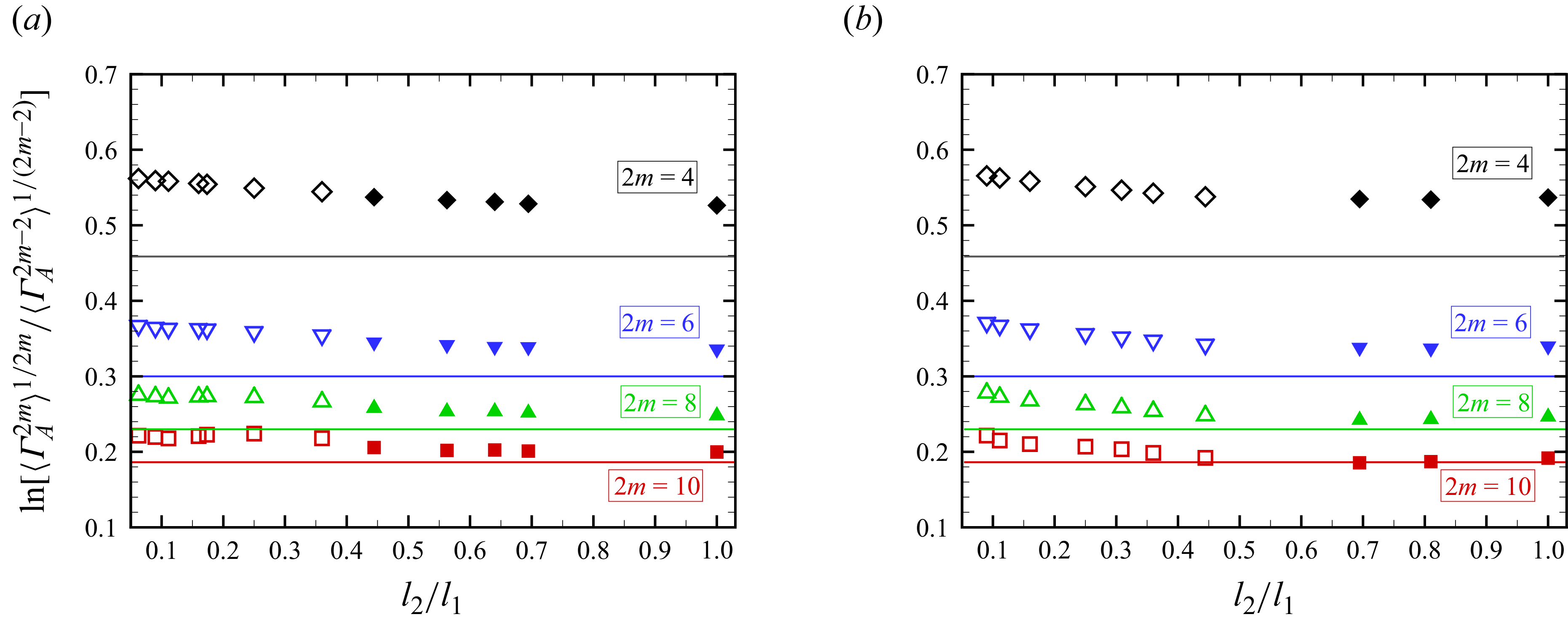
The logarithm of ratio of successive even-order circulation moments versus aspect ratio
 $l_2/l_1$
with a fixed area
 $A$
: (a)
 $y^+=40$
at
 $A/\eta ^2\approx 26\,000$
; (b)
 $y^+=0.3Re_\tau$
at
 $A/\eta ^2\approx 10\,000$
. Filled symbols correspond to
 $l_1$
and
 $l_2$
both inside the inertial range, and hollow symbols correspond to the rectangles with at least one side outside the inertial range. The horizontal lines correspond to equation (4) of Iyer et al. (Reference Iyer, Bharadwaj and Sreenivasan2021). Here,
 $ \textit{Re}_\tau =2000$
.

In figure 6 we examined the effect of aspect ratio on the low-order circulation moment, where recently Iyer et al. (Reference Iyer, Bharadwaj and Sreenivasan2021) showed that the validation of area rule may differ, particularly for the high orders. Following Iyer et al. (Reference Iyer, Bharadwaj and Sreenivasan2021), we examine the logarithm of the ratio of successive even-order moments
 $\mathrm{ln}[\langle \varGamma _A^{2m} \rangle ^{1/2m}/\langle \varGamma _A^{2m-2} \rangle ^{1/(2m-2)}]$
with varying aspect ratios, where
 $m$
is an integer and the loop-enclosed area
 $A$
is fixed. We show two examples in figure 7, one at
 $y^+=40$
(unifractality) in panel (a) and the other at
 $y^+=0.3Re_\tau$
(bifractality) in panel (b). As the order
 $2m$
increases, the ratios show better independence of the aspect ratio for both
 $y^+$
values. Iyer et al. (Reference Iyer, Bharadwaj and Sreenivasan2021) fit the tails of the circulation PDF using a gamma function to approximate the high even-order moments, and showed
 $\mathrm{ln}[\langle \varGamma _A^{2m} \rangle ^{1/2m}/\langle \varGamma _A^{2m-2} \rangle ^{1/(2m-2)}]\approx \mathrm{ln}[m/(m-1)]+\mathrm{ln}(4\pi m)/(4m) - \mathrm{ln}[4\pi (m-1)]/[4(m-1)]$
(see their equation 4), which is shown as solid lines in figure 7. As the order increases, our results approach the solid lines, and the agreement is quite good for
 $y^+=0.3Re_\tau$
, agreeing with the observations of Iyer et al. (Reference Iyer, Bharadwaj and Sreenivasan2021) in HIT and validating the area rule for the tails of the normalised circulation (Migdal Reference Migdal1994).
4. Conclusion
Exploring universal small-scale dynamics in turbulence is important, and two-point structure functions of velocity increments have shown that the universality in the inertial range is hindered by the intermittency. In the framework of Migdal (Reference Migdal1994), recent attempts have demonstrated that velocity circulation, a quantity associated with the velocity increments via the Stokes theorem, displays a bifractal feature, much simpler than the multi-fractal characteristics in the velocity increments (Iyer et al. Reference Iyer, Sreenivasan and Yeung2019; Müller et al. Reference Müller, Polanco and Krstulovic2021; Polanco et al. Reference Polanco, Müller and Krstulovic2021; Zhu et al. Reference Zhu, Xie and Xia2023). Importantly, the recent work of Duan et al. (Reference Duan, Chen and Sreenivasan2025) showed that the channel flow statistics of the area integral of the wall-normal vorticity component also exhibit bifractality, showing that this characteristic is not only the circumstance in ideal homogeneous turbulence but also in wall-bounded shear flow.
In this work, we demonstrate that this characteristic is also permitted in turbulent pipe flows, which have a curved wall, differing from the flat walls in channels. In cylindrical shells parallel to the pipe wall, we take the statistics of the velocity circulation, which equals to the area integral of the wall-normal vorticity via the Stokes theorem. The moments of the circulation show a bifractal singularity in the outer region, whereas they exhibit a unifractal non-singular behaviour in the inner region close to the wall. This makes for a close analogy with the statistics in channel flow, demonstrating that the geometric shape or azimuthal curvature in particular may not be a constraint factor to such statistics. The observed unifractality can be understood by examining how extreme events are suppressed. The viscous effects, which are strongest near the wall, suppress such extreme events, giving a more Gaussian PDF of the wall-normal vorticity. However, for the circulation with a small loop area, viscosity alone does not yield a fully Gaussian PDF. The remaining deviations from Gaussianity are progressively averaged out by integrating over a larger loop area (as evidenced from the kurtosis). In the inertial range, if the intermittency level is low, suppressed by the averaging effect, a unifractality is expected.
In our work, we selected data in a cylindrical shell mainly to fulfil the homogeneity condition, following the former studies. The validity of the area rule over loops enclosing non-homogeneous flows is less studied. Nevertheless, an approximate area rule was reported also in planes that are not parallel to the wall in contracting geometries (Mugundhan & Thoroddsen Reference Mugundhan and Thoroddsen2023). Since such planes will contain flow structures that are not naturally homogeneous, Mugundhan & Thoroddsen (Reference Mugundhan and Thoroddsen2023) finding suggests a broader generality of the area rule. Further studies with non-homogeneous flow data in other flow systems are needed to better evidence the generality.
Acknowledgements
D.X. would like to acknowledge Dr H. Li (Institute of Mechanics, Chinese Academy of Sciences) for insightful discussion. The authors also thank SuperComputing Network (SCNet) for providing the computing resources.
Funding
This work was supported by NSFC Excellence Research Group Program for ‘Multiscale Problems in Nonlinear Mechanics’ (No. 12588201), National Natural Science Foundation of China (Nos. 12372224, 92152106, 12322209 and 12272264) and Chinese Academy of Sciences (Project for Young Scientists in Basic Research, No. YSBR–087; Strategic Priority Research Program, No. XDB0620102).
Declaration of interests
The authors report no conflicts of interest.
Data availability statement
The data that support the findings of this study are available upon reasonable request to the corresponding author.
Author contributions
B.S.: performed simulation, wrote and reviewed the manuscript text. D.X.: conceptualised the study, analysed the data and prepared the figures and wrote and reviewed the manuscript.