1 Introduction
The motion of fluid through a domain with elastic boundaries has generated considerable attention, with applications including the re-opening of airways (Jensen et al. Reference Jensen, Horsburgh, Halpern and Gaver2002; Grotberg & Jensen Reference Grotberg and Jensen2004), the suppression of viscous fingering in a deformable Hele-Shaw cell (Pihler-Puzović et al. Reference Pihler-Puzović, Illien, Heil and Juel2012, Reference Pihler-Puzović, Périllat, Russel, Juel and Heil2013, Reference Pihler-Puzović, Juel, Peng, Lister and Heil2015; Al-Housseiny, Christov & Stone Reference Al-Housseiny, Christov and Stone2013), the adhesion of elastic elements (Hosoi & Mahadevan Reference Hosoi and Mahadevan2004) and the injection of viscous magma into the Earth’s crust, which leads to the formation of laccoliths (Bunger & Cruden Reference Bunger and Cruden2011; Michaut Reference Michaut2011). There has also been an increasing interest in the process of hydraulic fracturing owing to its importance for shale gas production, as well as in more conventional oil and gas reservoirs. Hydraulic fracturing is a complex process that involves the migration of a pressurised fluid into a fracture, such that, if the integrated stress of the fluid on the walls of the fracture exceeds the fracture toughness of the rock, then the fracture advances into the formation (Detournay Reference Detournay2016). However, if the walls of the fracture are permeable, then the fluid may be able to leak off into the formation, reducing the pressure within the fracture to such a degree that a quasi-steady balance can be established between the injection of fluid into the fracture and the subsequent leakage into the surrounding rock. In this limit, fracture growth is suppressed (Garagash & Detournay Reference Garagash and Detournay2000; Garagash, Detournay & Adachi Reference Garagash, Detournay and Adachi2011; Gordeliy & Detournay Reference Gordeliy and Detournay2011).
Although theoretical models have been developed and explored using analytical and numerical approaches, experimental modelling of hydraulic fracturing at a laboratory scale is difficult, and so there is value in developing a relatively simple analogue laboratory experiment from which some of the key principles and physical balances may be explored. Furthermore, there are a number of new challenges associated with the fate of particles in the fluid entering the fracture for which a well-characterised analogue system may provide an ideal experimental laboratory. The purpose of this paper is to develop a simple, analogue model of a hydraulic fracture based on the motion of a thin film of fluid injected between a permeable horizontal plate and an overlying, initially planar, elastic sheet, as shown in figure 1. Our aim is not to simulate the hydraulic fracturing process, but to characterise the motion of fluid injected between a porous plate and an elastic sheet. The elastic sheet provides a simplified, analogue model of the elastic stress on the walls of the fracture, while the porous plate allows for fluid to drain off, and thereby permits the establishment of a quasi-steady-state flow. Here, we characterise the dynamics controlling the motion of a viscous fluid injected into this model system by developing a theoretical model based on lubrication theory. In subsequent work we will present an experimental study of the system and explore some of the complexities associated, for example, with the injection of particles with the fluid.
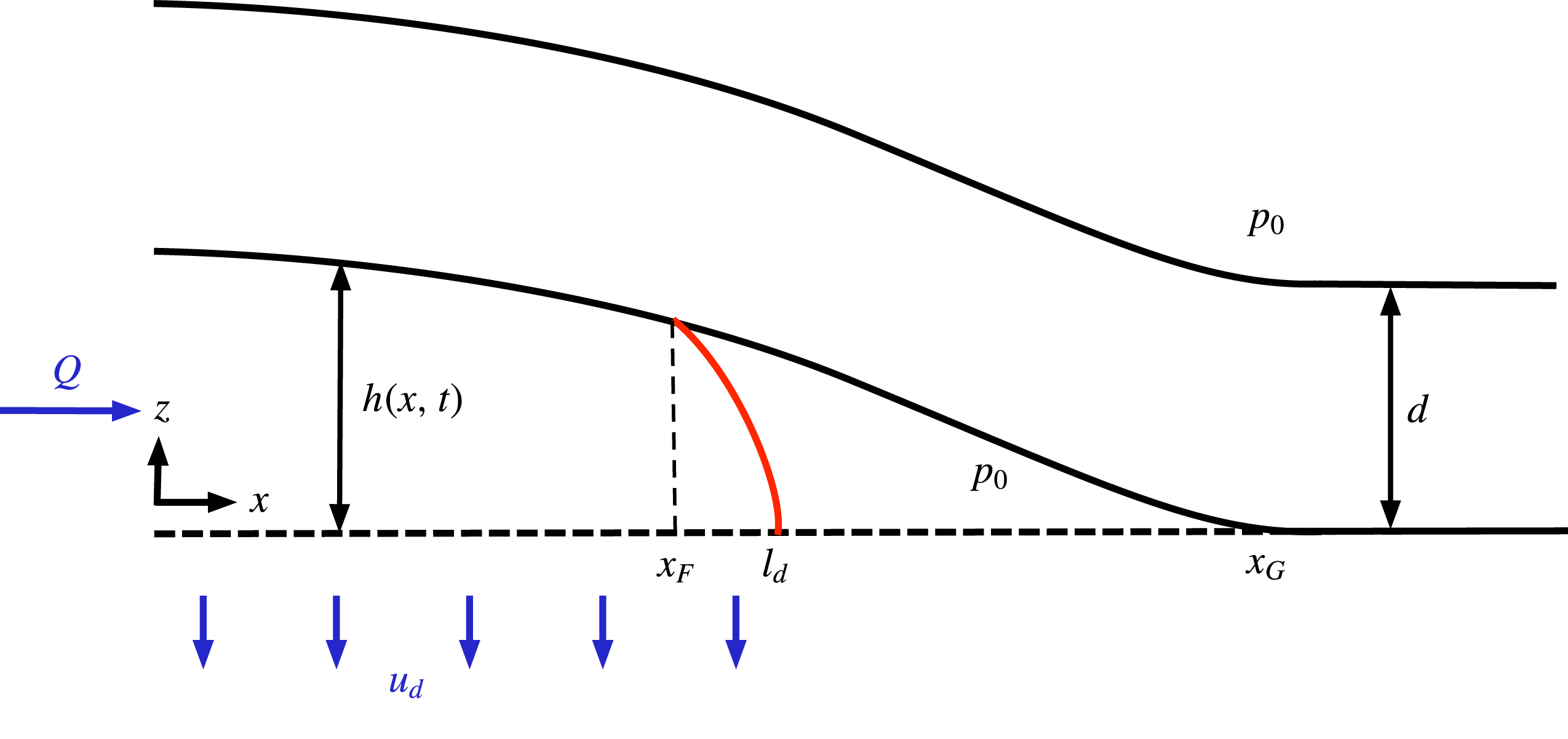
Schematic diagram of a current propagating below an elastic sheet with leakage. The figure indicates the coordinate system and illustrates the various dimensional variables. The red line denotes the profile of the current in the region
 $x_{F}<x<l_{d}$
. We consider that the fluid spreads laterally from the source in both the
 $+x$
and
 $-x$
directions; however, we exploit the mirror symmetry of the system about the injection point and consider only the
 $+x$
direction.

The motion of a fluid injected into a narrow gap between an elastic sheet and a rigid boundary has been explored by a number of authors, including Flitton & King (Reference Flitton and King2004), Pihler-Puzović et al. (Reference Pihler-Puzović, Illien, Heil and Juel2012, Reference Pihler-Puzović, Périllat, Russel, Juel and Heil2013, Reference Pihler-Puzović, Juel, Peng, Lister and Heil2015), Al-Housseiny et al. (Reference Al-Housseiny, Christov and Stone2013), Lister, Peng & Neufeld (Reference Lister, Peng and Neufeld2013), Hewitt, Balmforth & De Bruyn (Reference Hewitt, Balmforth and De Bruyn2015) and Peng et al. (Reference Peng, Pihler-Puzović, Juel, Heil and Lister2015). These analyses have focused on the transient growth of a fluid-filled fracture and have identified the need to regularise the evolution equation at the spreading tip. This tip region is then matched to the interior, where fluid flow is driven by pressure gradients associated with either gradients in the elastic stresses or the hydrostatic weight of the fluid. In the absence of a pre-existing fluid film, Flitton & King (Reference Flitton and King2004) showed that the propagation of the current is only possible because of complex physical processes at the front. Lister et al. (Reference Lister, Peng and Neufeld2013) regularised the problem by allowing for a pre-existing thin fluid film between the walls of the fracture. An interesting possibility, suggested by Hewitt et al. (Reference Hewitt, Balmforth and De Bruyn2015), is that a vapour- or air-filled region develops at the tip of the elastic sheet ahead of the advancing fluid region.
In this paper we explore the impact of the leakage of fluid through a permeable lower boundary as the fluid spreads between the boundary and the elastic sheet. To this end, we draw on the analysis of Acton, Huppert & Worster (Reference Acton, Huppert and Worster2001), Pritchard, Woods & Hogg (Reference Pritchard, Woods and Hogg2001) and Spannuth et al. (Reference Spannuth, Neufeld, Wettlaufer and Worster2009), for the dynamics of a viscous or porous gravity current flowing over a permeable boundary, but include the influence of the elastic stress from the deformable sheet. We now expect the system to reach an equilibrium state, in which the input flux matches the total drainage flux through a finite region of the lower boundary. To simplify the analysis, we assume that the drainage through the lower boundary has a constant flux per unit length
 $u_{d}$
so that the lateral extent of the drainage zone
 $l_{d}$
is given by the ratio of the input flux
 $Q$
and
 $u_{d}$
according to the relation
 $l_{d}=Q/u_{d}$
.
In order to determine the distribution of the fluid and the shape of the elastic sheet, we solve the coupled fluid–elastic system of equations. One complexity that arises is that, at some distance from the source,
 $x_{F}<l_{d}$
, the fluid separates from the elastic sheet, leading to an air- or ‘vapour’-filled zone,
 $x_{F}<x<x_{G}$
, where the plate is assumed to touch down at
 $x=x_{G}$
. Subsequently, in the region
 $x_{F}<x<l_{d}$
, the fluid spreads and drains as a pure viscous gravity current over the porous substrate (as shown in figure 1). Our interest lies in determining the controls on the magnitude of the upward displacement of the plate above the origin, the lateral extent of the fluid separation point,
 $x_{F}$
, and the touchdown point,
 $x_{G}$
, and the shape of the deformation of the elastic plate.
In order to identify the controlling dimensionless parameters, we consider simple scalings for the three forces acting on the fluid: (i) the weight of the elastic sheet,
 $\unicode[STIX]{x1D70C}_{s}gd$
, where
 $d$
is the thickness of the sheet and
 $\unicode[STIX]{x1D70C}_{s}$
the density of the sheet; (ii) the hydrostatic pressure,
 $\unicode[STIX]{x1D70C}gh$
, where
 $h$
is the depth of the fluid and
 $\unicode[STIX]{x1D70C}$
the density of the fluid; and (iii) the pressure associated with the elastic stress,
 $Bh/l_{d}^{4}$
, due to the curvature of the elastic sheet over the draining distance
 $l_{d}$
, where
 $h$
sets the scale for the deformation of the elastic plate of bending stiffness
 $B$
. In order to determine the ratio of these forces acting on the fluid, we require a scaling for
 $h$
. This may be found by observing that the horizontal flow over the draining distance
 $l_{d}$
is given by a balance of the viscous stress,
 $\unicode[STIX]{x1D707}u/h^{2}$
, and the gradient of either the hydrostatic pressure or elastic stress, or both, over the draining distance
 $l_{d}$
. If we use the elastic stress gradient, and recall that
 $hu\sim l_{d}u_{d}$
, then we obtain the scaling
 $h=(\unicode[STIX]{x1D707}u_{d}/B)^{1/4}l_{d}^{3/2}$
. In this case, the ratio of the weight of the elastic sheet per unit area and the elastic stress is given by
 $\unicode[STIX]{x1D706}=\unicode[STIX]{x1D70C}_{s}gdl_{d}^{4}/Bh$
, while the ratio of the hydrostatic pressure and the elastic stress is given by
 $P^{4}=l_{d}^{4}(\unicode[STIX]{x1D70C}g/B)$
. These two dimensionless parameters control the flow of the fluid and the deformation of the sheet. Note that when the hydrostatic pressure drives the flow, the ratio of the weight of the sheet to the hydrostatic pressure is given by
 $\unicode[STIX]{x1D706}/P^{5}$
. Although these parameters control the flow and deformation of the elastic sheet, the physical balances that determine the transitions from one limiting regime to another are somewhat subtle and require analysis of the coupled system of flow and elastic deformation. This is the focus of the present analysis.
Since the flow of the fluid along the sheet is driven by either the gravitational pressure gradient or the elastic pressure gradient, then the dynamics of the flow are controlled by one or other of these gradients, while the overall pressure in the fluid is controlled by the weight of the plate compared to the elastic and hydrostatic pressures. We can therefore infer some features of the general behaviour in different limiting cases, as follows. If
 $\unicode[STIX]{x1D706}\ll 1$
, then the weight of the sheet is small, and the dominant pressure will correspond to either the hydrostatic or elastic stress. In that case, one can envisage that, for
 $P\ll 1$
, there is an elastically driven flow in which the plate is in contact with the fluid nearly all the way to the end of the fluid region,
 $x=l_{d}$
, while for
 $x>l_{d}$
, the elevation of the plate gradually falls to zero over a distance that is large compared to
 $l_{d}$
. One can also envisage that for,
 $P\gg 1$
, there is a gravitationally driven flow in which the fluid drains as a viscous gravity current. Now, it may be that the fluid separates from the plate some distance upstream of the point
 $x=l_{d}$
. Again, the elevation of the plate will then gradually fall to zero over a length larger than
 $l_{d}$
. In contrast, if
 $\unicode[STIX]{x1D706}\gg \max (1,P^{5/2})$
, then in principle the weight of the sheet is relatively large and the dynamic pressure required to drive the fluid under the sheet is small. The fluid region will therefore have a nearly uniform, high pressure, which supports the plate. However, near the distal end of the flow, just before the point where the fluid separates from the sheet, the fluid pressure will decrease to much smaller values, leading to a small region across which there is a large viscous resistance as the pressure below the sheet falls to zero and, just before it touches down, the bending stress in the sheet supports its weight.
The purpose of the paper is to explore these different limiting cases in more detail, by developing a series of approximate or asymptotic solutions for the coupled flow and elastic deformation of the sheet. First, in § 2, we present a mathematical model of the flow below the sheet and the associated elastic deformation. We then explore the case
 $P\ll 1$
in § 3. We identify three regimes. First, we show that, in the case
 $P\ll \unicode[STIX]{x1D706}^{3/13}\ll 1$
, the hydrostatic pressure is negligible, and the point of separation of the fluid from the elastic sheet is virtually coincident with the end of the draining region. There is then a large region
 $x>l_{d}$
in which the elastic stress in the plate supports the weight of the plate until it eventually touches down. For fixed
 $P$
, as
 $\unicode[STIX]{x1D706}$
decreases through values such that
 $P\unicode[STIX]{x1D706}^{-3/13}=O(1)$
, the point of separation of the fluid from the plate gradually migrates backwards from the end of the draining zone towards the source, while the touchdown point still occurs far beyond the end of the draining zone. In contrast, for larger values of
 $\unicode[STIX]{x1D706}\gg 1$
, corresponding to the case in which the elastic plate is relatively heavy, the pressure beneath the plate is nearly constant. In this case, since the hydrostatic pressures are very small, the fluid only separates from the plate just upstream of the end of the draining zone. However, the pressure in the fluid has to decrease just before this point of separation in order to adjust to the low pressure of the air gap ahead of the fluid separation point. This is achieved through a viscous boundary layer just upstream of the end of the draining zone in which the fluid undergoes a significant drop in pressure. Owing to the weight of the sheet, the point of touchdown is very close to the end of the fluid draining zone.
In § 4 we explore the different regimes in which
 $P\gg 1$
, so that the gradient in hydrostatic pressure exceeds the gradient in elastic pressure driving the flow beneath the elastic sheet. We find that, when
 $\unicode[STIX]{x1D706}\gg P^{5/2}$
, the pressure in the fluid is virtually constant below the elastic sheet except in a small region just before the point of separation of the fluid from the sheet. Here the fluid pressure decreases rapidly to match the low pressure of the air gap which develops below the sheet just before it touches down. In this case, the point of separation of the fluid from the sheet occurs very close to the end of the draining zone. However, in the limit
 $\unicode[STIX]{x1D706}\ll P^{5/2}$
, the hydrostatic pressure dominates both the weight of the sheet and the elastic stresses in the sheet. As a result, the current resembles a classical gravity current, overlain by an elastic sheet, except in the nose of the flow, where the elastic stresses become comparable to the hydrostatic pressure as the sheet touches down. In § 5, we draw some conclusions and discuss the relevance of the model to provide insight into the related but distinct process of hydraulic fracturing.
2 Mathematical model
We consider the two-dimensional injection of a fluid between a deformable elastic sheet and a rigid, permeable substrate through which the fluid leaks off. A schematic diagram of the model system is shown in figure 1. The intrusion spreads laterally from the source in both the
 $+x$
and
 $-x$
directions; however, we exploit the symmetry of the system about the injection point and consider only the
 $+x$
direction. We assume that the horizontal extent of the flow is much greater than the vertical, and that the characteristic flow velocity is large in comparison with the leakage velocity, so that the flow is approximately parallel to the plate.
We assume that the point at which the fluid detaches from the elastic sheet,
 $x=x_{F}$
, lags the position at which the elastic sheet touches down on the substrate, at
 $x=x_{G}$
, and we define the size of the tip region
 $L=x_{G}-x_{F}$
. We also assume that the fluid detaches from the elastic sheet at
 $x=x_{F}<l_{d}<x_{G}$
. In the region
 $x_{F}<x<l_{d}$
, the fluid is driven forward as a conventional gravity current. The modelling of the three fluid regions is outlined below.
2.1 Fluid region in contact with the elastic sheet,
 $0<x<x_{F}$

We assume that the lateral extent of the fluid is much greater than the vertical deformation of the sheet, so that the flow is mainly horizontal. We also assume that the deflection of the sheet is small compared to the thickness of the sheet, such that deformation-induced in-plane stresses in the sheet are negligible compared to bending stresses, so that we can neglect the effect of any tension in the sheet. In the region
 $0<x<x_{F}$
, the pressure in the fluid is given by a combination of elastic bending stresses and the hydrostatic pressure, so that (Lister et al.
Reference Lister, Peng and Neufeld2013)
 $$\begin{eqnarray}p=p_{0}+\unicode[STIX]{x1D70C}_{s}gd+\unicode[STIX]{x1D70C}g(h-z)+B\frac{\unicode[STIX]{x2202}^{4}h}{\unicode[STIX]{x2202}x^{4}}.\end{eqnarray}$$
Here,
 $p_{0}$
is atmospheric pressure,
 $\unicode[STIX]{x1D70C}_{s}$
and
 $d$
are the density and thickness of the sheet respectively,
 $B=Ed^{3}/12(1-\unicode[STIX]{x1D708}^{2})$
is the bending stiffness of the sheet in terms of Young’s modulus
 $E$
and Poisson’s ratio
 $\unicode[STIX]{x1D708}$
,
 $\unicode[STIX]{x1D70C}$
is the fluid density, and
 $h(x,t)$
is the normal displacement of the sheet from its initial undeformed position.
Fluid flow beneath the elastic sheet, located at a height
 $h(x,t)$
above the porous substrate, is driven by horizontal gradients in the pressure and resisted by viscous drag resulting from the no-slip condition on the surfaces of the sheet and porous substrate. The local equation for the horizontal velocity
 $u(x,z,t)$
is therefore given by
 $$\begin{eqnarray}\unicode[STIX]{x1D70C}g\frac{\unicode[STIX]{x2202}h}{\unicode[STIX]{x2202}x}+B\frac{\unicode[STIX]{x2202}^{5}h}{\unicode[STIX]{x2202}x^{5}}=\unicode[STIX]{x1D707}\frac{\unicode[STIX]{x2202}^{2}u}{\unicode[STIX]{x2202}z^{2}}.\end{eqnarray}$$
Combining this with (2.1) leads to the expression for the volume flux per unit width,
 $q(x,t)$
,
 $$\begin{eqnarray}q(x,t)=-\frac{h^{3}}{12\unicode[STIX]{x1D707}}\left(\unicode[STIX]{x1D70C}g\frac{\unicode[STIX]{x2202}h}{\unicode[STIX]{x2202}x}+B\frac{\unicode[STIX]{x2202}^{5}h}{\unicode[STIX]{x2202}x^{5}}\right).\end{eqnarray}$$
Local conservation of mass then requires that
 $$\begin{eqnarray}\frac{\unicode[STIX]{x2202}h}{\unicode[STIX]{x2202}t}+\frac{\unicode[STIX]{x2202}q}{\unicode[STIX]{x2202}x}=-u_{d},\end{eqnarray}$$
where the drainage velocity is denoted
 $u_{d}$
. In practice, the drainage results from gravitational stresses associated with the weight of the sheet (
 $\unicode[STIX]{x1D70C}_{s}gd$
), the weight of the fluid in the porous substrate (
 $\unicode[STIX]{x1D70C}gb$
), where
 $b$
is the depth of the porous substrate), the depth of the injected fluid (
 $\unicode[STIX]{x1D70C}gh$
), the deformation-induced elastic stresses in the overlying sheet (
 $Bh^{(\text{iv})}$
) and the overall pressure jump from above the elastic sheet to the region below the porous substrate. In the remainder of this paper, we assume that the drainage velocity is a constant, so that the length over which drainage occurs is simply given by
 $l_{d}=Q/u_{d}$
, where
 $Q$
is the source flux. The simplification of a constant
 $u_{d}$
may apply, for example, in the case of a very heavy elastic sheet,
 $\unicode[STIX]{x1D70C}_{s}d\gg \unicode[STIX]{x1D70C}h$
, or in the case in which the weight of the fluid in the porous substrate dominates leakage, as occurs with a very deep substrate,
 $b\gg h$
. The time-dependent deformation of the elastic sheet can therefore be written as
 $$\begin{eqnarray}\frac{\unicode[STIX]{x2202}h}{\unicode[STIX]{x2202}t}-\frac{1}{12\unicode[STIX]{x1D707}}\frac{\unicode[STIX]{x2202}}{\unicode[STIX]{x2202}x}\left[h^{3}\frac{\unicode[STIX]{x2202}}{\unicode[STIX]{x2202}x}\left(\unicode[STIX]{x1D70C}gh+B\frac{\unicode[STIX]{x2202}^{4}h}{\unicode[STIX]{x2202}x^{4}}\right)\right]=-u_{d}.\end{eqnarray}$$
In the case of
 $u_{d}=0$
this agrees with the previous models of Lister et al. (Reference Lister, Peng and Neufeld2013) and Hewitt et al. (Reference Hewitt, Balmforth and De Bruyn2015). Here the addition of porous drainage introduces the possibility of a steady state. In this steady state, the height of the elastic plate above the porous substrate is given by
 $$\begin{eqnarray}\frac{1}{12\unicode[STIX]{x1D707}}\frac{\unicode[STIX]{x2202}}{\unicode[STIX]{x2202}x}\left[h^{3}\frac{\unicode[STIX]{x2202}}{\unicode[STIX]{x2202}x}\left(\unicode[STIX]{x1D70C}gh+B\frac{\unicode[STIX]{x2202}^{4}h}{\unicode[STIX]{x2202}x^{4}}\right)\right]=u_{d},\end{eqnarray}$$
subject to boundary conditions at the origin and point of separation of the fluid,
 $x=x_{F}$
. At the origin, the elasticity of the sheet requires that
 $$\begin{eqnarray}h^{\prime }(0)=h^{\prime \prime \prime }(0)=0,\end{eqnarray}$$
so there are no discontinuities or cusps in the sheet above the source, and that the bending moment of the sheet at the origin is zero. The second condition is a consequence of the assumption that the fluid spreads symmetrically from the source in both the
 $+x$
and
 $-x$
directions.
As
 $h^{\prime }(0)=0$
, the gradient of hydrostatic pressure at the origin is zero, and so the flux condition at
 $x=0$
is
 $$\begin{eqnarray}Q=-\left.\frac{Bh^{3}}{12\unicode[STIX]{x1D707}}\frac{\unicode[STIX]{x2202}^{5}h}{\unicode[STIX]{x2202}x^{5}}\right|_{x=0}.\end{eqnarray}$$
2.2 Air gap,
$x_{F}<x<x_{G}$

We assume that, beyond the point of separation of the elastic sheet and the fluid,
 $x>x_{F}$
, an air gap develops between the sheet and the porous substrate (cf. Hewitt et al.
Reference Hewitt, Balmforth and De Bruyn2015). In this region, we assume that the pressure of the air is atmospheric,
 $p_{0}$
, so that the weight of the plate is supported by the elastic stress in the plate,
 $$\begin{eqnarray}B\frac{\unicode[STIX]{x2202}^{4}h}{\unicode[STIX]{x2202}x^{4}}=-\unicode[STIX]{x1D70C}_{s}gd.\end{eqnarray}$$
The height of the sheet in the tip region is therefore
 $$\begin{eqnarray}h(x)=-\frac{\unicode[STIX]{x1D70C}_{s}gd}{24B}(x_{G}-x)^{3}(x_{F}-x)+h_{1}\frac{(x_{G}-x)^{3}}{L^{3}},\end{eqnarray}$$
where
 $x_{F}$
is the position at which the fluid detaches from the sheet,
 $x_{G}$
is the point where the sheet first touches the substrate,
 $L=x_{G}-x_{F}$
is the length of the tip region, and
 $h_{1}=h(x_{F})$
is the height of the sheet at the point of separation. We note that the quantities
 $L$
and
 $h_{1}$
, in addition to the deflection of the plate at the origin,
 $h_{0}$
, are to be found as part of the solution.
At the point of separation of the fluid from the plate, the deformation, gradient, bending moment and shear stress in the sheet and the pressure in the fluid provide a set of boundary conditions on the deformation of the sheet at the interface between the fluid region and the tip region:
 $$\begin{eqnarray}\displaystyle h(x_{F})\! & = & \displaystyle \!h_{1},\end{eqnarray}$$
 $$\begin{eqnarray}\displaystyle h^{\prime }(x_{F})\! & = & \displaystyle \!-3\frac{h_{1}}{L}+\frac{\unicode[STIX]{x1D70C}_{s}gd}{B}\frac{L^{3}}{24},\end{eqnarray}$$
 $$\begin{eqnarray}\displaystyle h^{\prime \prime }(x_{F})\! & = & \displaystyle \!6\frac{h_{1}}{L^{2}}-\frac{\unicode[STIX]{x1D70C}_{s}gd}{B}\frac{L^{2}}{4},\end{eqnarray}$$
 $$\begin{eqnarray}\displaystyle h^{\prime \prime \prime }(x_{F})\! & = & \displaystyle \!-6\frac{h_{1}}{L^{3}}+\frac{\unicode[STIX]{x1D70C}_{s}gd}{B}\frac{3L}{4},\end{eqnarray}$$
 $$\begin{eqnarray}\displaystyle h^{(\text{iv})}(x_{F})\! & = & \displaystyle \!-\frac{\unicode[STIX]{x1D70C}_{s}gd}{B}.\end{eqnarray}$$
2.3 Gravitationally driven drainage,
$x_{F}<x<l_{d}$

Finally, we note that there is a region of pure gravitationally driven flow beyond the point where the fluid separates from the elastic sheet. In this region,
 $x_{F}<x<l_{d}$
, the depth of the fluid is described by a model of a draining gravity current,
 $$\begin{eqnarray}\frac{\unicode[STIX]{x1D70C}g}{\unicode[STIX]{x1D707}}\frac{\unicode[STIX]{x2202}}{\unicode[STIX]{x2202}x}\left[f(x)h^{3}\frac{\unicode[STIX]{x2202}h}{\unicode[STIX]{x2202}x}\right]=u_{d},\end{eqnarray}$$
where the function
 $f(x)$
varies from
 $f(x_{F}^{+})\simeq 1/12$
immediately downstream of the detachment point, when the current resembles a no-slip current, to
 $f(x\rightarrow l_{d})\rightarrow 1/3$
further downstream once the current has adjusted to a free-slip pure gravity current. The transition region involves the adjustment of the current over a region of length
 $l_{\unicode[STIX]{x1D707}}\sim h(x_{F})g(\unicode[STIX]{x0394}\unicode[STIX]{x1D70C}gh^{3}/\unicode[STIX]{x1D707}^{2})$
, where
 $\unicode[STIX]{x0394}\unicode[STIX]{x1D70C}gh^{3}/\unicode[STIX]{x1D707}^{2}$
is a non-dimensional parameter describing the relaxation of the current to a free-slip surface through viscous diffusion, the determination of which is beyond the scope of the present paper. Depending on whether this length exceeds the distance between the point of separation and the end of the draining zone, the flow may more accurately be described by the no-slip value
 $f\simeq 1/12$
or the free-slip value
 $f\simeq 1/3$
. It is worth noting that at the detachment point,
 $x=x_{F}$
, there is a region in which the viscous flow transitions from one in which the sheet exerts a significant traction on the top surface to a free-surface, gravitationally driven flow. However, since for many solutions presented here
 $l_{d}-x_{F}\ll h(x_{F})\simeq l_{\unicode[STIX]{x1D707}}$
we take
 $f=1/12$
in the analysis in the present paper, and this leads to a lower-bound estimate for the length of the gravity draining flow. In this limit, the solution to (2.12) is given by
 $$\begin{eqnarray}h(x)=\left(\frac{48\unicode[STIX]{x1D707}}{\unicode[STIX]{x1D70C}g}\right)^{1/4}\left\{\frac{u_{d}}{2}[(x-x_{F})^{2}-(l_{d}-x_{F})^{2}]-q_{F}(x-l_{d})\right\}^{1/4},\end{eqnarray}$$
where
 $$\begin{eqnarray}q_{F}=-\frac{h_{1}^{3}}{12\unicode[STIX]{x1D707}}\left[\unicode[STIX]{x1D70C}g\frac{\unicode[STIX]{x2202}h}{\unicode[STIX]{x2202}x}+B\frac{\unicode[STIX]{x2202}^{5}h}{\unicode[STIX]{x2202}x^{5}}\right]_{x=x_{F}}\end{eqnarray}$$
is the flux through the last point of fluid contact with the elastic sheet,
 $x=x_{F}$
.
2.4 Non-dimensionalisation
We scale the horizontal lengths with the length scale over which drainage occurs,
 $\hat{x}=x/l_{d}$
, and vertical distances with the characteristic height of an elastically driven flow
 ${\hat{h}}=h/H$
, where
 $$\begin{eqnarray}H\equiv \left(\frac{12\unicode[STIX]{x1D707}u_{d}}{B}\right)^{1/4}l_{d}^{3/2}.\end{eqnarray}$$
The steady-state non-dimensional deformation of the sheet in the region in which the sheet is in contact with the fluid,
 $0<\hat{x}<\unicode[STIX]{x1D6FD}$
, is governed by
 $$\begin{eqnarray}\frac{\unicode[STIX]{x2202}}{\unicode[STIX]{x2202}\hat{x}}\left(P^{4}{\hat{h}}^{3}\frac{\unicode[STIX]{x2202}{\hat{h}}}{\unicode[STIX]{x2202}\hat{x}}+{\hat{h}}^{3}\frac{\unicode[STIX]{x2202}^{5}{\hat{h}}}{\unicode[STIX]{x2202}\hat{x}^{5}}\right)=1,\end{eqnarray}$$
where
 $$\begin{eqnarray}\unicode[STIX]{x1D6FD}\equiv \frac{x_{F}}{l_{d}}\quad \text{and}\quad P\equiv \frac{l_{d}}{(B/\unicode[STIX]{x1D70C}g)^{1/4}}\end{eqnarray}$$
are the non-dimensional length of the region of fluid–sheet contact, and the ratio of the hydrostatic pressure gradient to the bending stress exerted by the elastic sheet, respectively. The dimensionless flux condition at the origin takes the form
 $$\begin{eqnarray}{\hat{h}}^{3}{\hat{h}}^{(\text{v})}|_{0}=-1,\end{eqnarray}$$
along with conditions (cf. (2.7))
 $$\begin{eqnarray}{\hat{h}}^{\prime }(0)={\hat{h}}^{\prime \prime \prime }(0)=0.\end{eqnarray}$$
It is convenient to note that we can take the first integral of (2.16) subject to boundary conditions (2.18) and (2.19) to find
 $$\begin{eqnarray}{\hat{h}}^{3}\left(P^{4}\frac{\unicode[STIX]{x2202}{\hat{h}}}{\unicode[STIX]{x2202}\hat{x}}+\frac{\unicode[STIX]{x2202}^{5}{\hat{h}}}{\unicode[STIX]{x2202}\hat{x}^{5}}\right)=x-1,\end{eqnarray}$$
which describes the variation of the fluid flux under the sheet under the influence of buoyancy, an elastic sheet and distributed uniform drainage.
The dimensionless height of the sheet in the region in which the fluid is not in contact with the sheet,
 $\unicode[STIX]{x1D6FD}\leqslant \hat{x}\leqslant \unicode[STIX]{x1D6FD}+\hat{L}$
, is given by
 $$\begin{eqnarray}{\hat{h}}=-\frac{\unicode[STIX]{x1D706}}{24}(\unicode[STIX]{x1D6FD}+\hat{L}-\hat{x})^{3}(\unicode[STIX]{x1D6FD}-\hat{x})+{\hat{h}}_{\unicode[STIX]{x1D6FD}}\frac{(\unicode[STIX]{x1D6FD}+\hat{L}-\hat{x})^{3}}{\hat{L}^{3}},\end{eqnarray}$$
where
 $$\begin{eqnarray}\unicode[STIX]{x1D706}\equiv \frac{\unicode[STIX]{x1D70C}_{s}gd}{B}\frac{l_{d}^{4}}{H}\end{eqnarray}$$
is the ratio of the weight of the elastic sheet to the elastic stress in the fluid region, and
 $$\begin{eqnarray}\hat{L}=\frac{L}{l_{d}}=\frac{x_{G}-x_{F}}{l_{d}}\end{eqnarray}$$
is the dimensionless length of the tip region in which the fluid is not in contact with the sheet, and
 ${\hat{h}}_{\unicode[STIX]{x1D6FD}}=h_{1}/H$
. The boundary conditions at the interface between the fluid region and the tip region therefore have the dimensionless forms:
 $$\begin{eqnarray}\displaystyle {\hat{h}}(\unicode[STIX]{x1D6FD})\! & = & \displaystyle \!{\hat{h}}_{\unicode[STIX]{x1D6FD}},\end{eqnarray}$$
 $$\begin{eqnarray}\displaystyle {\hat{h}}^{\prime }(\unicode[STIX]{x1D6FD})\! & = & \displaystyle \!-\frac{3{\hat{h}}_{\unicode[STIX]{x1D6FD}}}{\hat{L}}+\frac{\hat{L}^{3}\unicode[STIX]{x1D706}}{24},\end{eqnarray}$$
 $$\begin{eqnarray}\displaystyle {\hat{h}}^{\prime \prime }(\unicode[STIX]{x1D6FD})\! & = & \displaystyle \!\frac{6{\hat{h}}_{\unicode[STIX]{x1D6FD}}}{\hat{L}^{2}}-\frac{\hat{L}^{2}\unicode[STIX]{x1D706}}{4},\end{eqnarray}$$
 $$\begin{eqnarray}\displaystyle {\hat{h}}^{\prime \prime \prime }(\unicode[STIX]{x1D6FD})\! & = & \displaystyle \!-\frac{6{\hat{h}}_{\unicode[STIX]{x1D6FD}}}{\hat{L}^{3}}+\frac{3\hat{L}\unicode[STIX]{x1D706}}{4},\end{eqnarray}$$
 $$\begin{eqnarray}\displaystyle {\hat{h}}^{(\text{iv})}(\unicode[STIX]{x1D6FD})\! & = & \displaystyle \!-\unicode[STIX]{x1D706}.\end{eqnarray}$$
 $\unicode[STIX]{x1D6FD}<\hat{x}<1$
is
 $$\begin{eqnarray}{\hat{h}}=\frac{2^{1/2}}{P}\left\{\frac{(\hat{x}-\unicode[STIX]{x1D6FD})^{2}}{2}-\frac{(1-\unicode[STIX]{x1D6FD})^{2}}{2}-(1-\unicode[STIX]{x1D6FD})(\hat{x}-1)\right\}^{1/4},\end{eqnarray}$$
where we have used (2.20) evaluated at
 $\hat{x}=\unicode[STIX]{x1D6FD}$
to determine the non-dimensional flux at the fluid–sheet detachment point. Evaluating this model of gravity slumping in the fluid-free tip at
 $\hat{x}=\unicode[STIX]{x1D6FD}$
further suggests that
 $$\begin{eqnarray}\unicode[STIX]{x1D6FD}=1-\frac{({\hat{h}}_{\unicode[STIX]{x1D6FD}}P)^{2}}{2^{1/2}},\end{eqnarray}$$
which determines the detachment length
 $\unicode[STIX]{x1D6FD}$
.
These conditions suggest that the height of the sheet at the point where the fluid separates from the elastic sheet scales with the length of the tip region ahead of this point,
 ${\hat{h}}_{\unicode[STIX]{x1D6FD}}\sim \unicode[STIX]{x1D706}\hat{L}^{4}$
. In the following analysis, we show that, in different regimes, the conditions in the tip region play dominant or subdominant roles in determining the deformation of the elastic sheet in the fluid-filled region. For clarity, we drop the hat notation and assume all variables are dimensionless from here onwards.
2.5 Numerical solution of the model equations
We determine the steady-state profile of the elastic sheet
 $h(x)$
by mapping (2.20) onto a domain for which
 $\tilde{x}\equiv x/x_{F}=[0,1]$
. The resultant, nonlinear fifth-order ordinary differential equation is solved with unknown
 $\unicode[STIX]{x1D6FD}$
,
 $h_{\unicode[STIX]{x1D6FD}}$
and
 $L$
subject to the eight boundary conditions (2.19), (2.24) and (2.26). Since the equations become numerically stiff near
 $\tilde{x}=1$
, we match to asymptotic solutions at
 $\tilde{x}=1-\unicode[STIX]{x1D700}$
(
 $\unicode[STIX]{x1D700}=10^{-7}$
for all the numerical solutions reported) and use continuation in the parameters
 $P$
and
 $\unicode[STIX]{x1D706}$
to obtain the full range of numerical solutions. Numerical solutions were determined using the routine bvp5c (in Matlab release R2016a, Mathworks, USA).
3 The limit of elastically driven flow,
$P\ll 1$

If
 $P\ll 1$
, the hydrostatic pressure is small, and the flow is driven by the elastic stresses. We hypothesise that the separation of the sheet occurs close to the end of the fluid draining zone,
 $\unicode[STIX]{x1D6FD}\sim 1$
, and that the deformation of the sheet is independent of hydrostatic pressure gradients. In the limit
 $P\ll 1$
, equation (2.20) is approximately
 $$\begin{eqnarray}h^{3}h^{(\text{v})}=x-1,\end{eqnarray}$$
and the solutions become independent of
 $P$
. The deformation of the sheet is now primarily controlled by
 $\unicode[STIX]{x1D706}$
, which represents the weight of the sheet compared to the elastic stress associated with the curvature of the sheet in the fluid region. Profiles of the height of the sheet
 $h(x)$
, normalised by the height of the sheet at the origin
 $h_{0}$
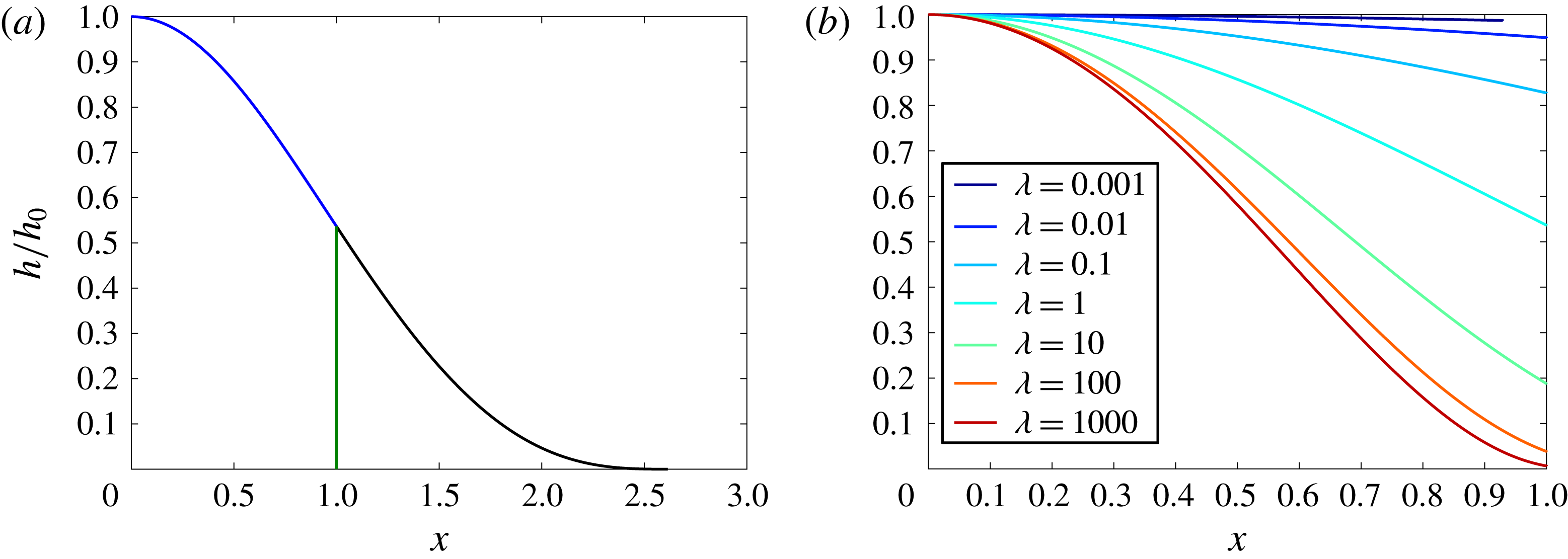
, are shown in figure 2(a) for
 $\unicode[STIX]{x1D706}=1$
and
 $P=0.1$
,
 $0.01$
and 0.001. The profiles collapse upon one another, corroborating the fact that, to leading order, in this regime the sheet deformation is independent of
 $P$
, and
 $1-\unicode[STIX]{x1D6FD}\ll \min (1,L)$
.
Profiles of the normalised height,
 $h(x)/h_{0}$
, in the fluid region are shown in figure 2(b) for
 $P=0.001$
and various values of
 $\unicode[STIX]{x1D706}$
in the range
 $0.001\leqslant \unicode[STIX]{x1D706}\leqslant 1000$
. For
 $\unicode[STIX]{x1D706}\gg 1$
, the pressure associated with the weight of the sheet far exceeds the change in pressure required to drive the liquid forward under the sheet over the lateral extent of the draining zone. As a result, the fluid pressure is nearly constant except in a boundary layer at the separation point, where the narrowing geometry of the gap leads to an increase in the viscous stress so that the fluid pressure adjusts from the high interior value to the low pressure within the tip. In this case, the plate touches down onto the substrate over a relatively short distance owing to the large weight of the plate compared to the elastic stress. In contrast, for
 $\unicode[STIX]{x1D706}\ll 1$
, the sheet is relatively light or stiff. As a result, the tip region is large compared to the fluid region and the change in height of the sheet from the injection point to the fluid front is small compared to the height of the sheet above the porous floor. This limit is analogous to the relaxation of an elastic sheet, under gravity, subject to a localised force near the origin. We now develop asymptotic solutions to describe these different regimes.
(a) The normalised sheet height
 $h/h_{0}$
as a function of distance
 $x$
in the fluid region (blue) and the tip region (black) as well as the gravity slumping front (green) for
 $\unicode[STIX]{x1D706}=1$
and
 $P=0.1$
, 0.01 and 0.001 for which
 $1-\unicode[STIX]{x1D6FD}=1.3\times 10^{-2}$
,
 $1.3\times 10^{-3}$
and
 $1.8\times 10^{-7}$
, respectively. The curves collapse on top of one another, suggesting that the normalised profiles are independent of
 $P$
. (b) Normalised sheet height
 $h/h_{0}$
as a function of distance
 $x$
in the fluid region for
 $P=0.001$
and various values of
 $\unicode[STIX]{x1D706}$
, as indicated in the legend, in the range
 $\unicode[STIX]{x1D706}=[0.001,1000]$
.

3.1 The light or stiff sheet:
$\unicode[STIX]{x1D706}\ll 1$

When elasticity dominates the flow and the sheet is either light or stiff,
 $P\ll 1$
and
 $\unicode[STIX]{x1D706}\ll 1$
, we expect that the change in depth of the sheet across the fluid region is small,
 $\unicode[STIX]{x0394}h=h_{0}-h_{\unicode[STIX]{x1D6FD}}\ll 1$
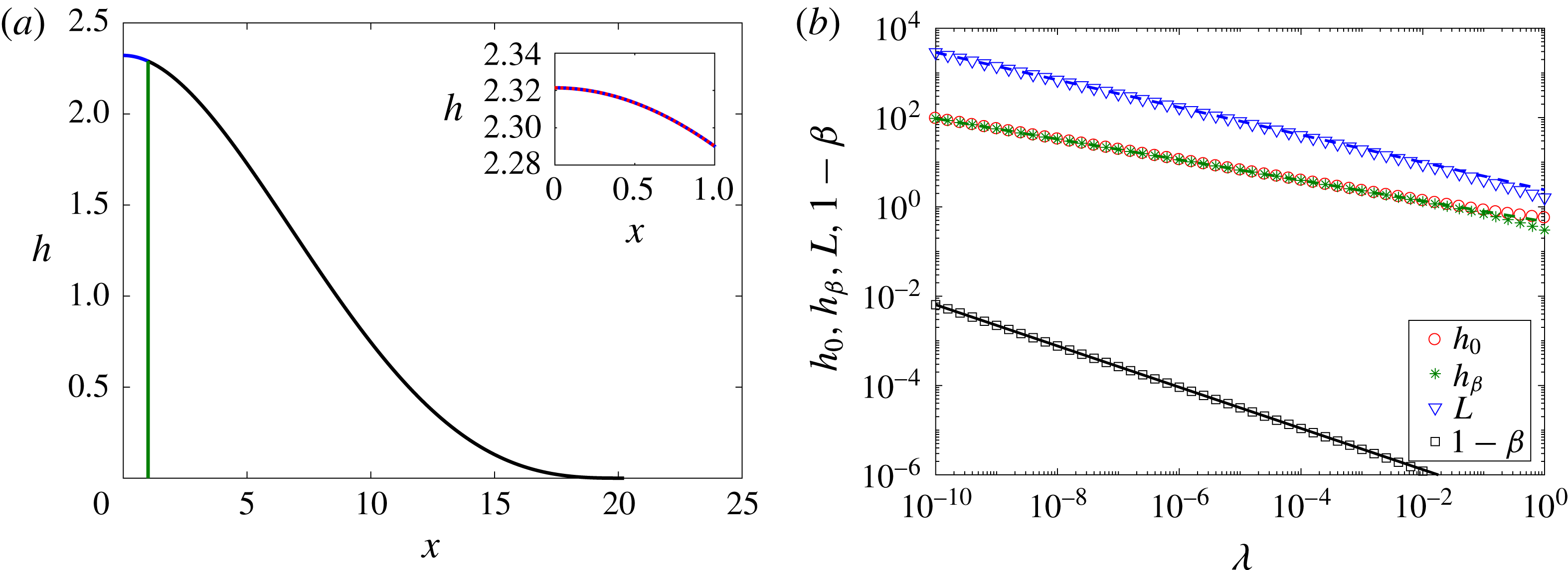
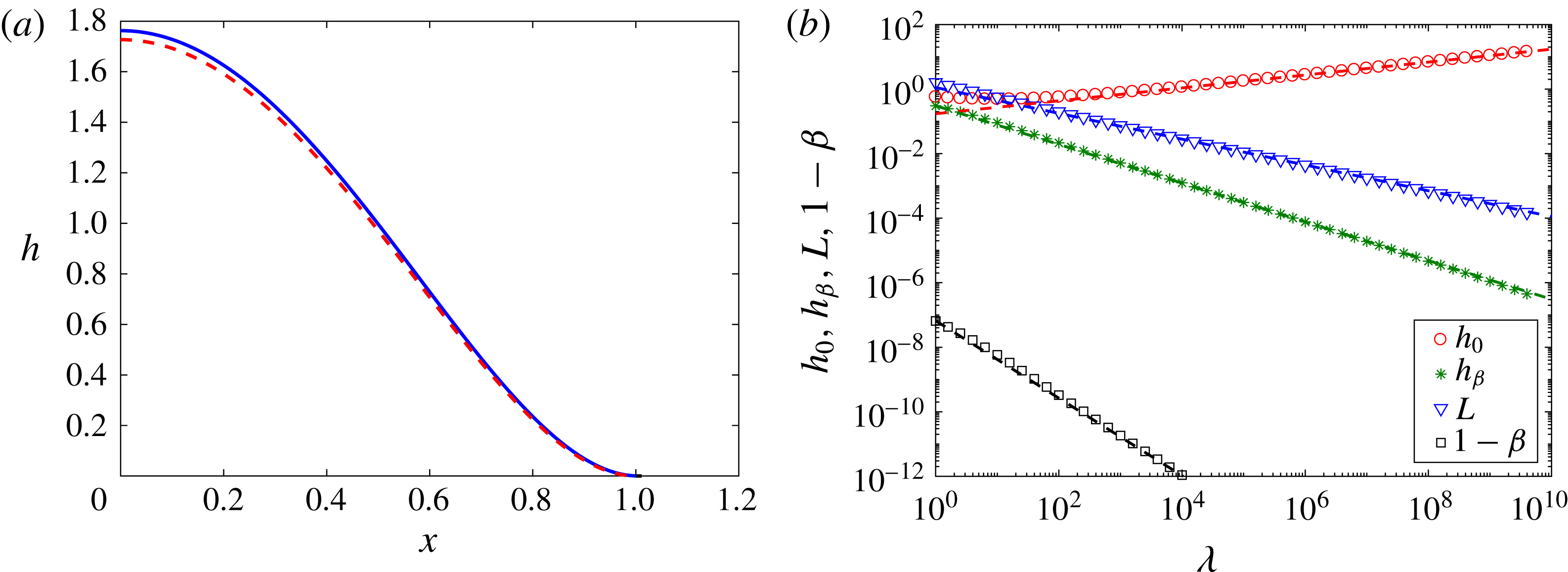
. A profile of the sheet height is shown in figure 3(a) for
 $P=0.001$
and
 $\unicode[STIX]{x1D706}=0.001$
. The length of the tip region is significantly greater than the length of the fluid region,
 $L\gg 1$
. In this limit, the fluid acts as a localised forcing that lifts the sheet from the substrate. The sheet only deforms appreciably under its own weight in the tip. In this limit we can linearise (3.1), subject to the boundary conditions at the origin, equation (2.19), and the bending stress at the point of separation of the fluid from the sheet,
 $h^{(\text{iv})}(\unicode[STIX]{x1D6FD})=-\unicode[STIX]{x1D706}$
. In developing an approximate solution, we also note that the detachment of the fluid from the sheet occurs at finite height
 $h_{\unicode[STIX]{x1D6FD}}$
. With these conditions we find that the height of the elastic sheet in the fluid region
 $0<x<1$
is approximated by
 $$\begin{eqnarray}h=h_{0}+\frac{1}{2h_{\unicode[STIX]{x1D6FD}}^{3}}\left(\frac{x^{6}}{360}-\frac{x^{5}}{60}+\frac{x^{4}}{24}\right)-\frac{\unicode[STIX]{x1D706}x^{4}}{24}+\frac{x^{2}}{2}\left(2(h_{\unicode[STIX]{x1D6FD}}-h_{0})-\frac{1}{36h_{\unicode[STIX]{x1D6FD}}^{3}}+\frac{\unicode[STIX]{x1D706}}{12}\right).\end{eqnarray}$$
This approximate solution for the height of the sheet in the fluid region is in good agreement with the numerically determined profile, as can be seen in figure 3(a) (inset) where the numerical and approximate solutions are almost indistinguishable. Evaluating (3.2) at the fluid front, and matching the deflection of the sheet and its first four derivatives, we find that
 $$\begin{eqnarray}\displaystyle h^{\prime }(\unicode[STIX]{x1D6FD})\! & = & \displaystyle \!-2\unicode[STIX]{x0394}h+\frac{1}{45h_{\unicode[STIX]{x1D6FD}}^{3}}-\frac{\unicode[STIX]{x1D706}}{12}=-\frac{3h_{\unicode[STIX]{x1D6FD}}}{L}+\frac{L^{3}\unicode[STIX]{x1D706}}{24},\end{eqnarray}$$
 $$\begin{eqnarray}\displaystyle h^{\prime \prime }(\unicode[STIX]{x1D6FD})\! & = & \displaystyle \!-2\unicode[STIX]{x0394}h+\frac{7}{72h_{\unicode[STIX]{x1D6FD}}^{3}}-\frac{5\unicode[STIX]{x1D706}}{12}=\frac{6h_{\unicode[STIX]{x1D6FD}}}{L^{2}}-\frac{L^{2}\unicode[STIX]{x1D706}}{4},\end{eqnarray}$$
 $$\begin{eqnarray}\displaystyle h^{\prime \prime \prime }(\unicode[STIX]{x1D6FD})\! & = & \displaystyle \!\frac{1}{6h_{\unicode[STIX]{x1D6FD}}^{3}}-\unicode[STIX]{x1D706}=-\frac{6h_{\unicode[STIX]{x1D6FD}}}{L^{3}}+\frac{3L\unicode[STIX]{x1D706}}{4},\end{eqnarray}$$
 $h_{0}=h_{\unicode[STIX]{x1D6FD}}=\unicode[STIX]{x1D706}L^{4}/72$
for
 $L\gg 1$
.
(a) The height
 $h$
of the sheet as a function of distance
 $x$
for
 $P=0.001$
and
 $\unicode[STIX]{x1D706}=0.001$
. In the fluid region, the analytic solution (3.2) is depicted by the red dashed line and the numerically calculated height profile is depicted by the blue line. The analytic solutions (2.21) and (2.25) are plotted for the sheet deformation in the tip region (black line) and the gravity slumping fluid front (green line), respectively. Inset: focusing in on the fluid region,
 $0\leqslant x\leqslant 1$
. (b) The height of the sheet at the origin,
 $h_{0}$
, and above the fluid front,
 $h_{\unicode[STIX]{x1D6FD}}$
, the length of the tip region,
 $L$
, and the length of the gravity slumping nose,
 $1-\unicode[STIX]{x1D6FD}$
(as indicated in the legend), calculated numerically as functions of
 $\unicode[STIX]{x1D706}$
, for
 $P=0.001$
and
 $\unicode[STIX]{x1D706}<1$
. Also shown are scalings for
 $h_{\unicode[STIX]{x1D6FD}}$
,
 $L$
and
 $1-\unicode[STIX]{x1D6FD}$
, given by (3.4) and represented by the green, blue and black dashed lines, respectively; to leading order,
 $h_{0}\sim h_{\unicode[STIX]{x1D6FD}}$
(3.6).

We now seek asymptotic expressions for
 $L$
,
 $h_{\unicode[STIX]{x1D6FD}}$
,
 $\unicode[STIX]{x0394}h$
and hence
 $h_{0}$
in terms of powers of
 $\unicode[STIX]{x1D706}$
in order to describe the control exerted by elasticity in the tip. Substituting
 $h_{\unicode[STIX]{x1D6FD}}\sim \unicode[STIX]{x1D706}L^{4}/72$
into (3.3c
), and neglecting lower-order terms in
 $L$
(here the term
 $-\unicode[STIX]{x1D706}$
), leads to the asymptotic expansions
 $$\begin{eqnarray}\displaystyle L\! & {\sim} & \displaystyle \!93\,312^{1/13}\unicode[STIX]{x1D706}^{-4/13},\end{eqnarray}$$
 $$\begin{eqnarray}\displaystyle h_{\unicode[STIX]{x1D6FD}}\! & {\sim} & \displaystyle \!{\textstyle \frac{93\,312^{4/13}}{72}}\unicode[STIX]{x1D706}^{-3/13},\end{eqnarray}$$
 $$\begin{eqnarray}\displaystyle 1-\unicode[STIX]{x1D6FD}\! & {\sim} & \displaystyle \!{\textstyle \frac{93\,312^{8/13}}{72^{2}\sqrt{2}}}P^{2}\unicode[STIX]{x1D706}^{-6/13}.\end{eqnarray}$$
 $\unicode[STIX]{x0394}h\sim 6h_{\unicode[STIX]{x1D6FD}}/L^{2}$
in (3.3b
) we find that
 $$\begin{eqnarray}\unicode[STIX]{x0394}h\sim {\textstyle \frac{93\,312^{2/13}}{12}}\unicode[STIX]{x1D706}^{5/13},\end{eqnarray}$$
which confirms that to leading order the deflection of the sheet above the injection point scales as
 $$\begin{eqnarray}h_{0}\sim h_{\unicode[STIX]{x1D6FD}}\sim {\textstyle \frac{93\,312^{4/13}}{72}}\unicode[STIX]{x1D706}^{-3/13}.\end{eqnarray}$$
The agreement between these scalings and the numerical calculations is shown in figure 3(b), and is surprisingly accurate, even for
 $P=1$
.
In the above analysis, we assumed that
 $\unicode[STIX]{x1D6FD}\simeq 1$
and so the interface between the fluid and the tip is vertical. The fluid will in fact separate from the elastic sheet at the point,
 $\unicode[STIX]{x1D6FD}<1$
, before reaching the fluid front (see § 2). In the region
 $\unicode[STIX]{x1D6FD}<x<1$
, the fluid will advance forward under gravity so that it reaches the point
 $x=1$
on the permeable plate. An estimate of the distance between the point of detachment of fluid from the elastic sheet and the fluid front,
 $1-\unicode[STIX]{x1D6FD}$
, is found by considering the drainage in a region of size
 $1-\unicode[STIX]{x1D6FD}$
driven by hydrostatic pressure,
 $(h^{3}h_{x})_{x}=P^{-4}$
, as given by (2.12). This leads to the relation
 $1-\unicode[STIX]{x1D6FD}\sim 2^{-1/2}(Ph_{\unicode[STIX]{x1D6FD}})^{2}$
and the prefactor can be found from recourse to (2.26) as given by (3.4c
) and shown in figure 3(b). Our assumption of a vertical fluid front is valid if the length scale of this gravitationally driven flow,
 $1-\unicode[STIX]{x1D6FD}$
, is much less than the length of the drainage region,
 $1-\unicode[STIX]{x1D6FD}\ll 1$
, and the length of the tip region,
 $1-\unicode[STIX]{x1D6FD}\ll L$
. Since
 $L\gg 1$
in this case, we only require that
 $1-\unicode[STIX]{x1D6FD}\ll 1$
so that
 $P\ll h_{\unicode[STIX]{x1D6FD}}^{-1}$
. Substituting in the scalings (3.4) for
 $h_{\unicode[STIX]{x1D6FD}}$
and
 $L$
, we find that this applies provided that
 $P\ll 72\unicode[STIX]{x1D706}^{3/13}/93\,312^{4/13}$
.
3.2 Separation of the fluid front from the touchdown position,
$1\gg P\gtrsim \unicode[STIX]{x1D706}^{3/13}$

In the limit that
 $P\geqslant 72\unicode[STIX]{x1D706}^{3/13}/93\,312^{4/13}$
, while
 $P\ll 1$
and
 $\unicode[STIX]{x1D706}\ll 1$
, then
 $1-\unicode[STIX]{x1D6FD}$
is no longer small, and the point of separation of the fluid from the elastic sheet migrates back from the end of the draining zone to the point
 $x=\unicode[STIX]{x1D6FD}<1$
. Now, generalising the previous solution, it follows that the height of the elastic sheet in the fluid region
 $0<x<\unicode[STIX]{x1D6FD}$
is approximated by
 $$\begin{eqnarray}h=h_{0}+\frac{1}{2h_{\unicode[STIX]{x1D6FD}}^{3}}\left(\frac{x^{6}}{360}-\unicode[STIX]{x1D6FD}\frac{x^{5}}{60}+\unicode[STIX]{x1D6FD}^{2}\frac{x^{4}}{24}\right)-\frac{\unicode[STIX]{x1D706}x^{4}}{24}+\frac{x^{2}}{2\unicode[STIX]{x1D6FD}^{2}}\left(2(h_{\unicode[STIX]{x1D6FD}}-h_{0})-\frac{\unicode[STIX]{x1D6FD}^{6}}{36h_{\unicode[STIX]{x1D6FD}}^{3}}+\frac{\unicode[STIX]{x1D706}\unicode[STIX]{x1D6FD}^{4}}{12}\right).\end{eqnarray}$$
Using this solution in the boundary conditions at
 $x=\unicode[STIX]{x1D6FD}$
, we find that
 $$\begin{eqnarray}\displaystyle h^{\prime }(\unicode[STIX]{x1D6FD})\! & = & \displaystyle \!-\frac{2\unicode[STIX]{x0394}h}{\unicode[STIX]{x1D6FD}}+\frac{\unicode[STIX]{x1D6FD}^{5}}{45h_{\unicode[STIX]{x1D6FD}}^{3}}-\frac{\unicode[STIX]{x1D706}\unicode[STIX]{x1D6FD}^{3}}{12}=-\frac{3h_{\unicode[STIX]{x1D6FD}}}{L}+\frac{L^{3}\unicode[STIX]{x1D706}}{24},\end{eqnarray}$$
 $$\begin{eqnarray}\displaystyle h^{\prime \prime }(\unicode[STIX]{x1D6FD})\! & = & \displaystyle \!-\frac{2\unicode[STIX]{x0394}h}{\unicode[STIX]{x1D6FD}^{2}}+\frac{7\unicode[STIX]{x1D6FD}^{4}}{72h_{1}^{3}}-\frac{5\unicode[STIX]{x1D706}\unicode[STIX]{x1D6FD}^{2}}{12}=\frac{6h_{\unicode[STIX]{x1D6FD}}}{L^{2}}-\frac{L^{2}\unicode[STIX]{x1D706}}{4},\end{eqnarray}$$
 $$\begin{eqnarray}\displaystyle h^{\prime \prime \prime }(\unicode[STIX]{x1D6FD})\! & = & \displaystyle \!\frac{\unicode[STIX]{x1D6FD}^{3}}{6h_{\unicode[STIX]{x1D6FD}}^{3}}-\unicode[STIX]{x1D706}=-\frac{6h_{\unicode[STIX]{x1D6FD}}}{L^{3}}+\frac{3L\unicode[STIX]{x1D706}}{4}.\end{eqnarray}$$
 $$\begin{eqnarray}\displaystyle h_{\unicode[STIX]{x1D6FD}}\! & = & \displaystyle \!\frac{L^{4}\unicode[STIX]{x1D706}}{72},\end{eqnarray}$$
 $$\begin{eqnarray}\displaystyle L & {\sim} & \displaystyle 93\,312^{1/13}\unicode[STIX]{x1D706}^{-4/13}\unicode[STIX]{x1D6FD}^{3/13},\end{eqnarray}$$
 $$\begin{eqnarray}\displaystyle \unicode[STIX]{x0394}h=h_{0}-h_{\unicode[STIX]{x1D6FD}} & {\sim} & \displaystyle {\textstyle \frac{93\,312^{2/13}}{12}}\unicode[STIX]{x1D706}^{5/13}\unicode[STIX]{x1D6FD}^{2}.\end{eqnarray}$$
Finally, we can constrain the relationship between
 $\unicode[STIX]{x1D6FD}$
and
 $h_{\unicode[STIX]{x1D6FD}}$
using the solution for the gravitationally driven flow in the region
 $\unicode[STIX]{x1D6FD}<x<1$
given by (2.25) and recalling the relationship (2.26) between
 $h_{\unicode[STIX]{x1D6FD}}$
and
 $\unicode[STIX]{x1D6FD}$
. Combining (2.26) with (3.9a,b
) leads to the implicit relation for
 $\unicode[STIX]{x1D6FD}$
in terms of
 $P$
and
 $\unicode[STIX]{x1D706}$
as given by
 $$\begin{eqnarray}\frac{(1-\unicode[STIX]{x1D6FD})^{1/2}}{\unicode[STIX]{x1D6FD}^{12/13}}=\frac{93\,312^{4/13}}{72\times 2^{1/4}}P\unicode[STIX]{x1D706}^{-3/13}.\end{eqnarray}$$
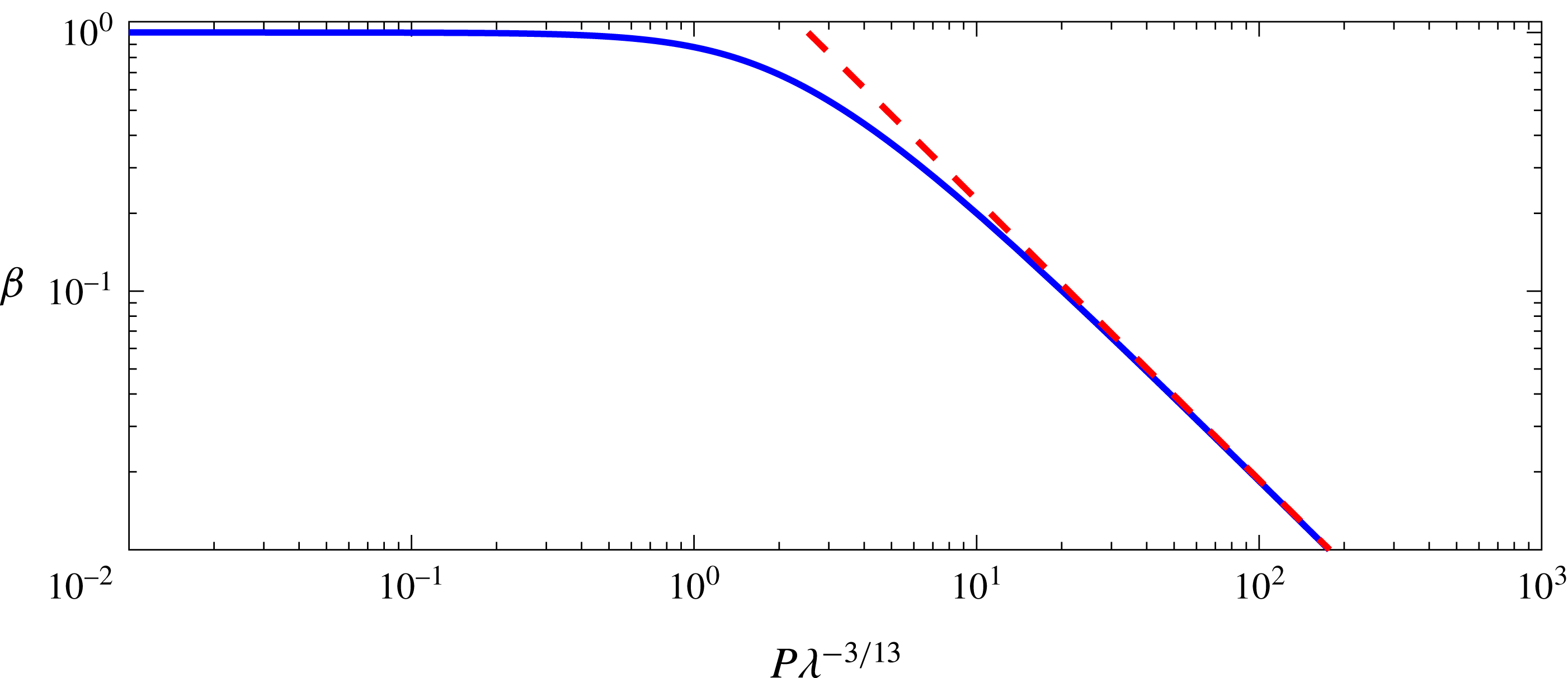
This relation illustrates how the separation point of the fluid migrates back towards the source as
 $P\unicode[STIX]{x1D706}^{-3/13}$
progressively increases and the gravity slumping of the fluid ahead of the point of separation becomes more significant, as shown in figure 4.
The separation point as a function of
 $P\unicode[STIX]{x1D706}^{-3/13}$
from the solution of (3.10), and where the red dashed line indicates the asymptotic limit
 $\unicode[STIX]{x1D6FD}\simeq (2.5315/P\unicode[STIX]{x1D706}^{-3/13})^{13/12}$
.

As
 $\unicode[STIX]{x1D706}$
increases for a given
 $P(\ll 1)$
and the weight of the elastic plate increases, the point of touchdown of the plate migrates back towards the distal end of the draining zone,
 $x=1$
, and eventually the tip region, of length
 $L$
, becomes small relative to the draining zone,
 $L\ll 1$
. This leads to the next series of cases in which we explore the behaviour of a relatively heavy plate,
 $\unicode[STIX]{x1D706}\gg 1$
, for various values of
 $P$
.
3.3 The heavy or flexible sheet:
$\unicode[STIX]{x1D706}\gg 1$

When
 $\unicode[STIX]{x1D706}\gg 1$
, the weight of the sheet is much greater than the elastic stress associated with the pressure gradient required to drive the fluid under the sheet. Now the sheet deforms readily under its own weight, and so the length of the tip region,
 $\unicode[STIX]{x1D6FD}<x<\unicode[STIX]{x1D6FD}+L$
, is expected to be much smaller than the length of the fluid region,
 $L\ll 1$
. The pressure gradients needed to drive fluid from the source over the porous substrate are small compared to the background pressure associated with supporting the weight of the sheet. The pressure is therefore nearly constant within the main interior of the fluid. In contrast, near the point of separation of the fluid from the sheet, the viscous stresses become significant since a large pressure gradient is needed to drive the viscous fluid into the narrowing confines of the gap and thus match the low pressure in the air tip. In considering the asymptotic behaviour for
 $\unicode[STIX]{x1D706}\gg 1$
, we match the nearly uniform pressure of the fluid below the sheet to a viscous boundary layer near the point of separation. As in the earlier solutions, since
 $P\ll 1$
, we expect that the distance between the separation point and the end of the draining zone is small, so we make the simplification
 $\unicode[STIX]{x1D6FD}\approx 1$
; again, we check the validity of this approximation by checking that
 $(1-\unicode[STIX]{x1D6FD})\ll \min (1,L)$
once we have developed the asymptotic solutions.
In the interior, the variation of the height of the plate follows the approximate relation
 $h^{(\text{v})}\sim h_{0}^{-3}$
and so, for
 $\unicode[STIX]{x1D706}\gg 1$
, we find that the fluid pressure is nearly constant,
 $h_{p}^{(\text{iv})}=K$
, where
 $K$
depends on the details of the flow and elastic deformation near the point of separation of the fluid from the plate. Since the height and gradient of the sheet
 $h(\unicode[STIX]{x1D6FD})=h^{\prime }(\unicode[STIX]{x1D6FD})=\mathit{O}(h_{\unicode[STIX]{x1D6FD}})$
at
 $x=\unicode[STIX]{x1D6FD}$
, an approximate solution for the sheet is
 $$\begin{eqnarray}h=\frac{K}{24}(\unicode[STIX]{x1D6FD}-x^{2})^{2}.\end{eqnarray}$$
Near the point of separation of the fluid from the plate (near
 $x=\unicode[STIX]{x1D6FD}$
), the height of the sheet is
 $\mathit{O}(h_{\unicode[STIX]{x1D6FD}})$
, and the viscous stresses dominate over an adjustment region with length scale
 $L_{t}$
. In this boundary layer, we expect solutions of the form,
 $h=h_{\unicode[STIX]{x1D6FD}}f(\unicode[STIX]{x1D701}=(x-\unicode[STIX]{x1D6FD})/L_{t})$
such that (3.1) becomes
 $$\begin{eqnarray}f^{3}f^{(\text{v})}=\unicode[STIX]{x1D701},\end{eqnarray}$$
and the tip length scale is related to the height at the point of separation of the fluid,
 $L_{t}=h_{\unicode[STIX]{x1D6FD}}^{2/3}$
, by a scaling of (3.1). In the case
 $P\ll 1$
, for which gravity is small, we expect that
 $\unicode[STIX]{x1D6FD}\sim 1$
and hence solve (3.12) subject to rescaled boundary equations at the fluid front,
 $\unicode[STIX]{x1D701}=0$
, to find that
 $$\begin{eqnarray}\displaystyle f(0)\! & = & \displaystyle \!1,\end{eqnarray}$$
 $$\begin{eqnarray}\displaystyle f^{\prime }(0)\! & = & \displaystyle \!a\left(-3+\frac{b}{24}\right),\end{eqnarray}$$
 $$\begin{eqnarray}\displaystyle f^{\prime \prime }(0)\! & = & \displaystyle \!a^{2}\left(6-\frac{b}{4}\right),\end{eqnarray}$$
 $$\begin{eqnarray}\displaystyle f^{\prime \prime \prime }(0)\! & = & \displaystyle \!a^{3}\left(-6+\frac{3b}{4}\right),\end{eqnarray}$$
 $$\begin{eqnarray}\displaystyle f^{(\text{iv})}(0)\! & = & \displaystyle \!-a^{4}b,\end{eqnarray}$$
 $a=L_{t}/L$
, and tip pressure has been scaled to give
 $b=\unicode[STIX]{x1D706}L^{4}/h_{\unicode[STIX]{x1D6FD}}$
. In order for this boundary layer solution to match onto the interior solution, we require that the curvature tends to a constant, and so we set
 $$\begin{eqnarray}f^{\prime \prime \prime },f^{(\text{iv})}\rightarrow 0\quad \text{as }\unicode[STIX]{x1D701}\rightarrow -\infty .\end{eqnarray}$$
Solution of the boundary layer problem for
 $f(\unicode[STIX]{x1D701})$
thus yields a value for
 $K$
, the interior fluid pressure. Using Matlab’s bvp5c function, we solved this boundary layer problem taking
 $\unicode[STIX]{x1D6FD}=1$
and in this case we find that
 $a=0.4058$
,
 $b=5.1325$
and
 $f^{\prime \prime }(\unicode[STIX]{x1D701}\rightarrow -\infty )=0.9311$
. This leads to the solution for the interior pressure,
 $$\begin{eqnarray}K=3(ba^{4})^{-1/5}f^{\prime \prime }(-\infty )\unicode[STIX]{x1D706}^{1/5},\end{eqnarray}$$
and hence that
 $$\begin{eqnarray}\displaystyle h_{\unicode[STIX]{x1D6FD}}\! & = & \displaystyle \!(ba^{4})^{3/5}\unicode[STIX]{x1D706}^{-3/5}=0.3063\unicode[STIX]{x1D706}^{-3/5},\end{eqnarray}$$
 $$\begin{eqnarray}\displaystyle L\! & = & \displaystyle \!b^{2/5}a^{3/5}\unicode[STIX]{x1D706}^{-2/5}=1.1197\unicode[STIX]{x1D706}^{-2/5},\end{eqnarray}$$
 $$\begin{eqnarray}\displaystyle h_{0}\! & = & \displaystyle \!\frac{(ba^{4})^{-1/5}}{8}f^{\prime \prime }(-\infty )\unicode[STIX]{x1D706}^{1/5}=0.1727\unicode[STIX]{x1D706}^{1/5},\end{eqnarray}$$
 $$\begin{eqnarray}\displaystyle 1-\unicode[STIX]{x1D6FD}\! & = & \displaystyle \!\frac{(0.3063\unicode[STIX]{x1D706}^{-3/5}P)^{2}}{\sqrt{2}},\end{eqnarray}$$
 $P=0.001$
and
 $\unicode[STIX]{x1D706}=1000$
.
These scalings and numerical values for the height of the sheet above the origin,
 $h_{0}$
, and at the fluid front,
 $h_{\unicode[STIX]{x1D6FD}}$
, the length of the tip region,
 $L$
, and the gravity slumping nose,
 $1-\unicode[STIX]{x1D6FD}$
, calculated as functions of
 $\unicode[STIX]{x1D706}$
, are shown in figure 5(b) for
 $\unicode[STIX]{x1D706}>1$
. The length of this gravity current scales as
 $1-\unicode[STIX]{x1D6FD}\sim (Ph_{\unicode[STIX]{x1D6FD}})^{2}/2$
and so, in order that the solution is self-consistent, we require
 $1-\unicode[STIX]{x1D6FD}\ll \min (1,L)$
. From our scalings for
 $h_{\unicode[STIX]{x1D6FD}}$
and
 $L$
, equations (3.16a
)–(3.16b
), we find that the condition
 $1-\unicode[STIX]{x1D6FD}\ll 1$
requires
 $P\ll \unicode[STIX]{x1D706}^{3/5}$
. Also, the condition that
 $1-\unicode[STIX]{x1D6FD}\ll L$
requires
 $P\ll \unicode[STIX]{x1D706}^{2/5}$
. These are always satisfied in the case
 $P\ll 1$
while
 $\unicode[STIX]{x1D706}\gg 1$
, and so the approximation
 $\unicode[STIX]{x1D6FD}\approx 1$
is self-consistent, as demonstrated by the numerical solutions in figure 5(b).
(a) The height
 $h$
of the sheet as a function of distance
 $x$
for
 $P=0.001$
and
 $\unicode[STIX]{x1D706}=1000$
. In the fluid region, the approximate solution (3.11) for a constant pressure interior is depicted by the red dashed line and the numerically calculated height profile is depicted by the blue line. (b) The height of the sheet at the origin,
 $h_{0}$
, and above the fluid front,
 $h_{\unicode[STIX]{x1D6FD}}$
, the length of the tip region,
 $L$
, and the length of the gravity slumping nose,
 $1-\unicode[STIX]{x1D6FD}$
(as indicated in the legend), calculated numerically as functions of
 $\unicode[STIX]{x1D706}$
, for
 $P=0.001$
and
 $\unicode[STIX]{x1D706}>1$
. Also shown are scalings for
 $h_{0}$
(red),
 $h_{\unicode[STIX]{x1D6FD}}$
(green),
 $L$
(blue) and
 $1-\unicode[STIX]{x1D6FD}$
(black) given by (3.16a
)–(3.16d
).

4 Gravitationally driven flows:
$P\gg 1$

When
 $P\gg 1$
, the hydrostatic pressure dominates the elastic stress over the length scale across which the fluid drains. There are then two limits, which we explore below. When the hydrostatic pressure is moderate compared to the weight of the elastic plate,
 $\unicode[STIX]{x1D706}\gg 1$
, we anticipate that, as in § 3.3, the pressure within the main body of fluid will be nearly constant, but that now there is a region of length
 $1/P$
in which elastic stresses become significant, upstream of the point of separation of the fluid from the sheet. In this boundary layer the curvature becomes large and the elastic stresses dominate the hydrostatic pressure, in an analogous fashion to § 3.3. We develop a model for this regime, and then find that
 $\unicode[STIX]{x1D706}\gg P^{5/2}$
for this solution to be self-consistent. In contrast, with a lighter elastic sheet, for which
 $\unicode[STIX]{x1D706}\ll P^{5/2}$
, the hydrostatic pressure dominates within the current, and the flow then behaves in a similar fashion to a classical gravity current with the elastic sheet following the profile of a gravity current. In this limit, flow is driven by hydrostatic pressure gradients through to the detachment point, and the effects of elasticity are only important in determining the structure of the sheet in the tip region.
(a) The normalised height profile of the sheet
 $h/h_{0}$
for
 $P=10$
and for various values of
 $\unicode[STIX]{x1D706}$
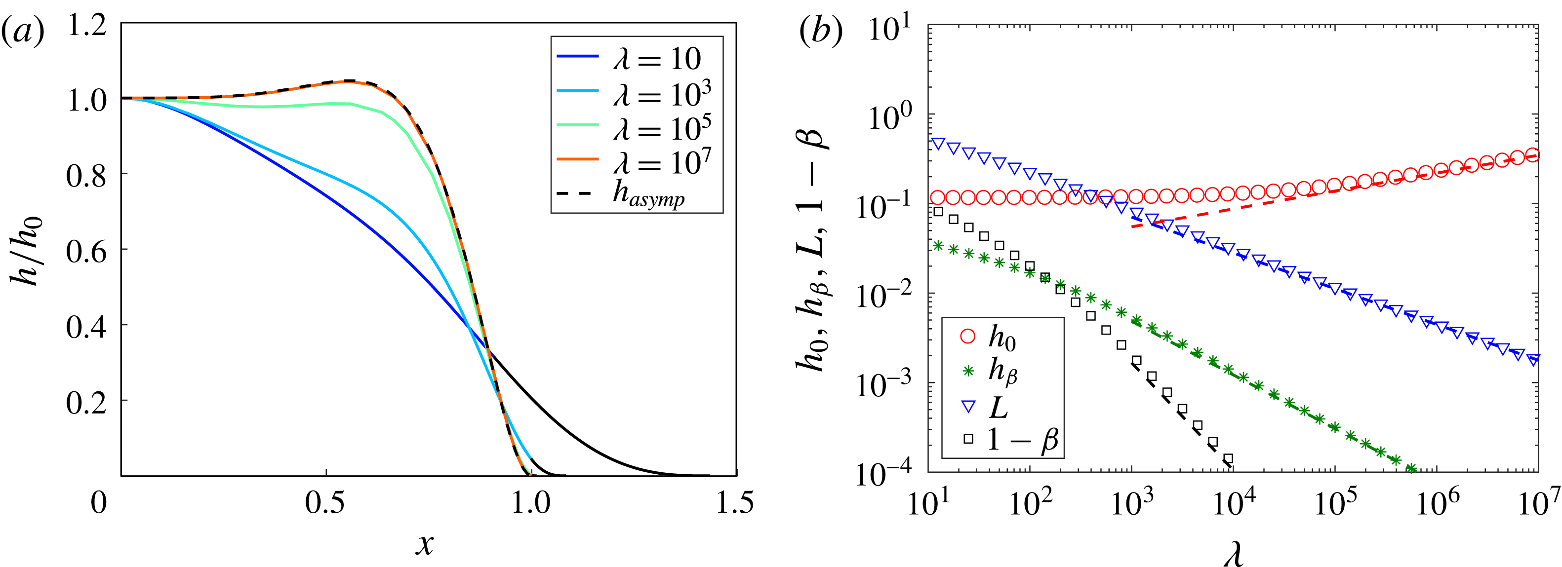
(as indicated in the legend), along with the asymptotic solution (dashed) given by (4.4). The coloured lines indicate the fluid region and the corresponding black lines represent the tip region. (b) Plot showing
 $h_{0}$
,
 $h_{\unicode[STIX]{x1D6FD}}$
,
 $L$
and
 $1-\unicode[STIX]{x1D6FD}$
as functions of
 $\unicode[STIX]{x1D706}$
for
 $P=10$
. Markers represent the numerical computations (as indicated in the legend) and the scalings for
 $h_{0}$
(red),
 $h_{\unicode[STIX]{x1D6FD}}$
(green),
 $L$
(blue) and
 $1-\unicode[STIX]{x1D6FD}$
(black) given by (4.7a
)–(4.7d
) are also included for comparison.

4.1 Elasticity dominates at the point of fluid separation:
$1\ll P\ll \unicode[STIX]{x1D706}^{2/5}$

For intermediate values of
 $P$
, both gravity and elasticity play a role in determining the profile of the sheet. As in the elastic case, the pressure gradients needed to drive fluid towards the fluid front are small compared with the pressure that lifts the sheet off the permeable substrate. In this limit the pressure within the fluid is nearly constant, as given by
 $h^{(\text{iv})}+P^{4}h=K$
where, as in § 3.3,
 $K$
is to be found from the conditions at the front of the flow. Since the height and deflection of the sheet are small at the point where the fluid separates from the sheet (
 $x=\unicode[STIX]{x1D6FD}$
), then
 $h(\unicode[STIX]{x1D6FD})=h^{\prime }(\unicode[STIX]{x1D6FD})=\mathit{O}(h_{\unicode[STIX]{x1D6FD}})$
, and the leading-order solution for the deflection of the sheet is
 $$\begin{eqnarray}h=h_{0}[1+a\cos \unicode[STIX]{x1D709}\cosh \unicode[STIX]{x1D709}+b\sin \unicode[STIX]{x1D709}\sinh \unicode[STIX]{x1D709}],\end{eqnarray}$$
where
 $$\begin{eqnarray}\unicode[STIX]{x1D709}=\frac{\unicode[STIX]{x1D701}}{\sqrt{2}/P}\end{eqnarray}$$
and
 $$\begin{eqnarray}a=-\frac{\cosh \unicode[STIX]{x1D6FE}\sin \unicode[STIX]{x1D6FE}+\cos \unicode[STIX]{x1D6FE}\sinh \unicode[STIX]{x1D6FE}}{\cos \unicode[STIX]{x1D6FE}\sin \unicode[STIX]{x1D6FE}+\cosh \unicode[STIX]{x1D6FE}\sinh \unicode[STIX]{x1D6FE}},\quad b=\frac{\csc \unicode[STIX]{x1D6FE}\,\text{csch}\,\unicode[STIX]{x1D6FE}(\cot \unicode[STIX]{x1D6FE}-\coth \unicode[STIX]{x1D6FE})}{\coth \unicode[STIX]{x1D6FE}\csc \unicode[STIX]{x1D6FE}^{2}+\cot \unicode[STIX]{x1D6FE}\,\text{csch}\,\unicode[STIX]{x1D6FE}^{2}},\end{eqnarray}$$
and where
 $\unicode[STIX]{x1D6FE}=\unicode[STIX]{x1D6FD}P/\sqrt{2}$
. In the limit
 $P\gg 1$
this takes the far simpler expression
 $$\begin{eqnarray}h=h_{0}\{1-\text{e}^{\unicode[STIX]{x1D709}-\unicode[STIX]{x1D6FE}}[\cos (\unicode[STIX]{x1D6FE}-\unicode[STIX]{x1D709})+\sin (\unicode[STIX]{x1D6FE}-\unicode[STIX]{x1D709})]\},\end{eqnarray}$$
in which we have taken
 $h^{\prime }(0)=h^{\prime \prime \prime }(0)\rightarrow 0$
in the asymptotic limit
 $P^{-1}\rightarrow 0$
. This asymptotic solution is shown alongside numerical profiles of the height of the sheet in figure 6(a), calculated for various values of
 $\unicode[STIX]{x1D706}$
, and corroborates that
 $h/h_{0}$
becomes non-monotonic for intermediate values of
 $P$
and large
 $\unicode[STIX]{x1D706}$
.
At the point of separation of the fluid from the sheet, where the deflection of the sheet matches onto the tip region, the elastic stresses dominate as described by the boundary layer solutions described in § 3.3. Here, as before, the relationship between the boundary layer length scale and the fluid height has the form
 $L_{t}=h_{\unicode[STIX]{x1D6FD}}^{3/2}$
and we expect that
 $\unicode[STIX]{x1D6FD}\approx 1$
. Following the analysis of § 3.3, we define
 $a=L_{t}/L$
and
 $b=\unicode[STIX]{x1D706}L^{4}/h_{\unicode[STIX]{x1D6FD}}$
and find that
 $a=0.4058$
,
 $b=5.1325$
and
 $f^{\prime \prime }(\unicode[STIX]{x1D701}\rightarrow -\infty )=0.9311$
. Now matching the curvature of the elastically dominated fluid front to the interior solution we find that
 $$\begin{eqnarray}h_{\unicode[STIX]{x1D709}\unicode[STIX]{x1D709}}|_{\unicode[STIX]{x1D709}\rightarrow \unicode[STIX]{x1D6FE}}=\frac{P^{2}h_{0}}{2}\left[\frac{-2+\cos 4\unicode[STIX]{x1D6FE}+\cosh 4\unicode[STIX]{x1D6FE}}{(\sin 2\unicode[STIX]{x1D6FE}+\sinh 2\unicode[STIX]{x1D6FE})^{2}}\right]=\frac{h_{\unicode[STIX]{x1D6FD}}}{L_{t}^{2}}f^{\prime \prime }(-\infty ).\end{eqnarray}$$
In the limit
 $P\gg 1$
, this simplifies to
 $$\begin{eqnarray}h_{\unicode[STIX]{x1D709}\unicode[STIX]{x1D709}}|_{\unicode[STIX]{x1D709}\rightarrow \unicode[STIX]{x1D6FE}}=P^{2}h_{0}=\frac{h_{\unicode[STIX]{x1D6FD}}}{L_{t}^{2}}f^{\prime \prime }(-\infty ),\end{eqnarray}$$
and hence we find, with
 $1\ll P\ll \unicode[STIX]{x1D706}^{2/5}$
, that
 $$\begin{eqnarray}\displaystyle h_{1}\! & = & \displaystyle \!(ba^{4})^{3/5}\unicode[STIX]{x1D706}^{-3/5}=0.3063\,\unicode[STIX]{x1D706}^{-3/5},\end{eqnarray}$$
 $$\begin{eqnarray}\displaystyle L\! & = & \displaystyle \!b^{2/5}a^{3/5}\unicode[STIX]{x1D706}^{-2/5}=1.1197\,\unicode[STIX]{x1D706}^{-2/5},\end{eqnarray}$$
 $$\begin{eqnarray}\displaystyle h(0)\! & = & \displaystyle \!b^{-1/5}a^{-4/5}f^{\prime \prime }(-\infty )P^{-2}\unicode[STIX]{x1D706}^{1/5}=1.3813\,P^{-2}\unicode[STIX]{x1D706}^{1/5},\end{eqnarray}$$
 $$\begin{eqnarray}\displaystyle 1-\unicode[STIX]{x1D6FD}\! & = & \displaystyle \!\frac{(0.3063\unicode[STIX]{x1D706}^{-3/5}P)^{2}}{\sqrt{2}}.\end{eqnarray}$$
 $h_{0}$
,
 $h_{\unicode[STIX]{x1D6FD}}$
,
 $L$
and
 $1-\unicode[STIX]{x1D6FD}$
as functions of
 $\unicode[STIX]{x1D706}$
for
 $P=10$
in figure 6(b).
However, in the limit
 $P\unicode[STIX]{x1D706}^{-2/5}\sim 1$
, flow near the fluid detachment point is driven by both elastic and hydrostatic pressure gradients. The ratio
 $P\unicode[STIX]{x1D706}^{-2/5}$
gradually increases, hydrostatic pressure gradients become progressively more important within the tip until eventually they dominant, and only a small elastic region determines the touchdown point of the sheet in advance of the fluid detachment point, as considered in the next section.
4.2 Gravity dominates at the point of fluid separation:
$P\gg \unicode[STIX]{x1D706}^{2/5}$

For
 $P\gg \unicode[STIX]{x1D706}^{2/5}$
, with
 $P\gg 1$
, the hydrostatic pressure dominates over the elastic stress and the weight of the plate, so the solution is analogous to a classical gravity current. However, at the end of the draining zone, the plate also touches down, and so there is a region near the nose where the elastic stress becomes important and hence affects this touchdown. Upstream of the nose of the flow, the solution is given by the gravity current solution of the equation
 $$\begin{eqnarray}P^{4}h^{3}h^{\prime }=x-1,\end{eqnarray}$$
as given by
 $$\begin{eqnarray}h=2^{1/4}\frac{(1-x)^{1/2}}{P},\end{eqnarray}$$
where, since the flow is at all times predominantly driven by gravity, we impose
 $h(x\rightarrow 1)=0$
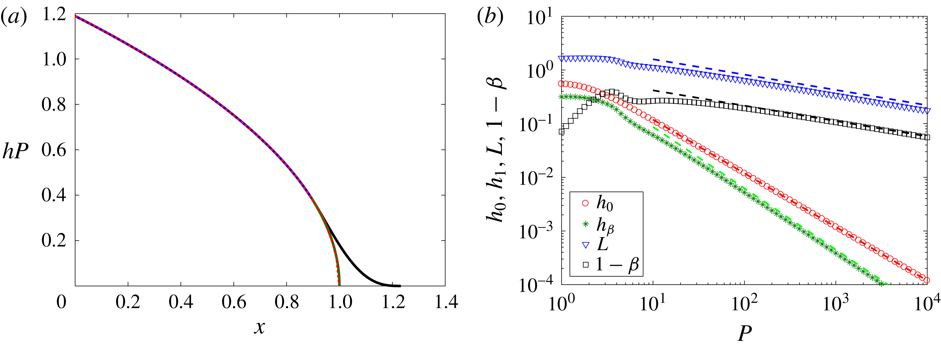
. A comparison of this asymptotic solution with the full numerical solution for the deflection of the sheet is shown in figure 7(a) for
 $P=1000$
and
 $\unicode[STIX]{x1D706}=1$
. The figure demonstrates the excellent agreement between the asymptotic and full numerical solutions.
Furthermore, we see that, because hydrostatic pressure gradients dominate through to the fluid detachment point, the solution (4.9) remains an excellent approximation throughout. This implies that
 $$\begin{eqnarray}h_{\unicode[STIX]{x1D6FD}}=\frac{2^{1/4}}{P}(1-\unicode[STIX]{x1D6FD})^{1/2},\end{eqnarray}$$
and hence, from boundary condition (2.24e ), that the detachment point
 $$\begin{eqnarray}1-\unicode[STIX]{x1D6FD}=\left(\frac{16}{15}\frac{\unicode[STIX]{x1D706}P}{2^{1/4}}\right)^{-2/7}.\end{eqnarray}$$
We may similarly write an expression for the fluid height at the detachment point,
 $$\begin{eqnarray}h_{\unicode[STIX]{x1D6FD}}=\frac{2^{1/4}}{P}\left(\frac{16}{15}\frac{\unicode[STIX]{x1D706}P}{2^{1/4}}\right)^{-1/7}.\end{eqnarray}$$
Finally, we note that from (4.9) and (2.24b ) the following quartic polynomial for the length of the vapour tip is suggested:
 $$\begin{eqnarray}L=6\left({\textstyle \frac{16}{15}}{\textstyle \frac{1}{2^{1/4}}}\right)^{-2/7}\!(\unicode[STIX]{x1D706}P)^{-2/7}-{\textstyle \frac{2^{3/4}}{24}}\left({\textstyle \frac{16}{15}}{\textstyle \frac{1}{2^{1/4}}}\right)^{-1/7}\!(\unicode[STIX]{x1D706}P)^{6/7}L^{4},\end{eqnarray}$$
which depends solely on
 $\unicode[STIX]{x1D706}P$
. We note that, in the two asymptotic limits,
 $$\begin{eqnarray}L\simeq \left\{\begin{array}{@{}rcll@{}}6\left({\textstyle \frac{16}{15}}{\textstyle \frac{1}{2^{1/4}}}\right)^{-2/7}\!(\unicode[STIX]{x1D706}P)^{-2/7}\, & =\, & 6.1894(\unicode[STIX]{x1D706}P)^{-2/7}, & \quad \unicode[STIX]{x1D706}P<1,\\ \left[{\textstyle \frac{144}{2^{3/4}}}\left({\textstyle \frac{16}{15}}{\textstyle \frac{1}{2^{1/4}}}\right)^{-1/7}\right]^{1/4}\!(\unicode[STIX]{x1D706}P)^{-2/7}\, & =\, & 3.0538(\unicode[STIX]{x1D706}P)^{-2/7}, & \quad \unicode[STIX]{x1D706}P>1.\end{array}\right.\end{eqnarray}$$
We compare these asymptotic solutions (dashed lines) against the full numerical solutions (symbols) in figure 7(b) for
 $\unicode[STIX]{x1D706}=1$
and
 $P\gg 1$
corresponding to the limit
 $\unicode[STIX]{x1D706}P>1$
in (4.14).
The height
 $h$
of the elastic sheet as a function of distance
 $x$
for
 $P=1000$
and
 $\unicode[STIX]{x1D706}=1$
. In the fluid region
 $x=[0,1]$
, both the numerically calculated (blue line) height and the analytic solution (red dashed line) for a gravity current, equation (4.9), are depicted (taking
 $h_{1}\rightarrow 0$
) along with the analytic solution (2.21) for the sheet in the vapour tip
 $x=[1,1+L]$
(black line). (b) The height of the sheet at the origin,
 $h_{0}$
, and the fluid at detachment,
 $h_{\unicode[STIX]{x1D6FD}}$
, and the length of the tip region,
 $L$
, and gravity nose,
 $1-\unicode[STIX]{x1D6FD}$
, as functions of
 $P$
for
 $\unicode[STIX]{x1D706}=1$
. Numerical findings are denoted by the markers, as indicated in the legend, and compared with scaling relationships for
 $h_{0}$
(red),
 $h_{\unicode[STIX]{x1D6FD}}$
(green),
 $L$
(blue) and
 $1-\unicode[STIX]{x1D6FD}$
(black) given by (4.9) evaluated at
 $x=0$
, and (4.12), (4.14) and (4.11).

5 Discussion and conclusions
We have examined the injection of liquid from a point source into the gap between an elastic sheet and a permeable horizontal base in a planar geometry. We have found that a family of steady-state draining solutions arise as anticipated by balances between elastically or gravitationally driven flow and leakage. The flow from the source to the region over the permeable base in which there is drainage is controlled by either (i) the horizontal gravitational pressure gradient associated with the decreasing thickness of the fluid layer with distance from the source or (ii) the elastic stress associated with the deformation of the elastic sheet. We have also found that, beyond the draining region, there is a transition region in which the elastic sheet touches down onto the permeable base. This transition region is controlled by a balance between the weight of the elastic sheet and its bending moment, with the boundary condition that the elastic stress in the sheet is continuous at the point that the fluid separates from the sheet.
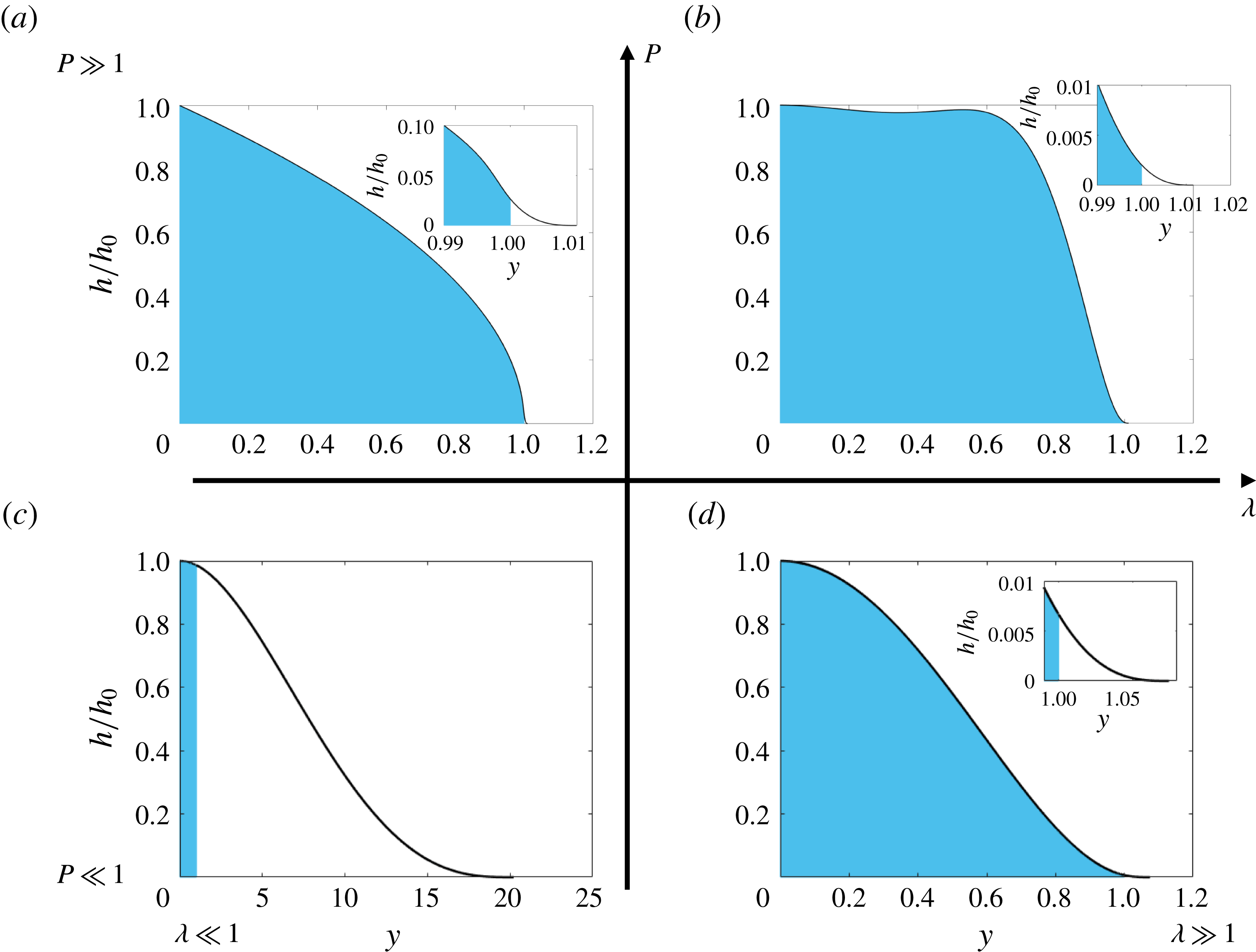
In the case that the gravitational pressure gradient in the fluid drives the flow and the sheet is relatively light compared to the fluid, the depth of the flow reduces rapidly to zero near the front of the flow and the sheet is drawn down close to the horizontal plane (figure 8 a). If, instead, the sheet is denser than the fluid, then elastic effects become important in the fluid region before the fluid has detached from the sheet and dramatically alter the shape of the sheet from one similar to the profile of a gravity current (figure 8 b). Both of these cases lead to a very short transition zone relative to the draining length of the flow as, in one, the sheet is drawn close to the horizontal plane and, in the other, the sheet readily deforms under its own weight. However, in the case that the flow is driven by the elastic stresses, the gravitational stress associated with the fluid acts over a much larger scale than the elastic stress and so, if the sheet is relatively light, then the touchdown distance is relatively large compared to the drainage length (figure 8 c), and the touchdown problem resembles one in which a sheet is propped up near the origin and drapes down to the plane. In contrast, if the elastic sheet is much denser than the fluid, then the touchdown length becomes smaller than the drainage scale (figure 8 d).
Illustrative profiles of the sheet deformation regions for the various limits of
 $P=l_{d}(\unicode[STIX]{x1D70C}g/B)^{1/4}$
, where
 $l_{d}$
is the extent of the fluid film,
 $B$
the bending stiffness of the sheet,
 $\unicode[STIX]{x1D70C}$
the density of the fluid, and
 $\unicode[STIX]{x1D706}=(\unicode[STIX]{x1D70C}_{s}gd/B)(l_{d}^{4}/H)$
, where
 $\unicode[STIX]{x1D70C}_{s}$
is the density of the sheet,
 $H=(12\unicode[STIX]{x1D707}u_{d}/B)^{1/4}l_{d}^{3/2}$
,
 $\unicode[STIX]{x1D707}$
is the dynamic viscosity of the fluid and
 $u_{d}$
is the drainage velocity through the permeable substrate. In each of (a)–(d) the solid black line represents the sheet while the shaded blue area and the unshaded area beneath the sheet indicate the fluid region and the tip region, respectively. Note that the formal limits distinguishing the different regimes are described in the main text.

In the analysis included in §§ 3 and 4, we have developed asymptotic expressions for the shape of the elastic sheet and for the lateral extent of the touchdown distance in each of these cases. We note that the model has some similarities to the work of Lister et al. (Reference Lister, Peng and Neufeld2013) and Hewitt et al. (Reference Hewitt, Balmforth and De Bruyn2015), in that they predicted a transition from an elastically dominated flow at early times, when the deformation and fluid region are small, to a gravitationally dominated flow at long times, when the deformation and fluid region are large. In the present problem, with a steady-state flow and drainage through the lower boundary, the parameter
 $P$
has a similar influence in determining the flow regime, in that, with a large drainage region,
 $P$
is large and the system is controlled by the gravitational stress, whereas, with small
 $P$
, the drainage region is relatively small and the flow is controlled by the elastic stresses.
An important simplification in our analysis was the neglect of the tension in the elastic sheet, which is valid provided that the stress associated with the tension in the sheet is small compared to the stress associated with the bending moment of the sheet, and this requires that
 $h^{2}/d^{2}\ll 1$
, where
 $d$
is the thickness of the sheet. The above results predict the following in the various regimes for
 $P$
and
 $\unicode[STIX]{x1D706}$
: (i)
 $P\ll 1$
and
 $\unicode[STIX]{x1D706}\ll 1$
, the maximum deflection of the light/stiff sheet from the initial undeformed position occurs above the injection point and follows the scaling
 $h_{0}\sim 93\,312^{4/13}\unicode[STIX]{x1D706}^{-3/13}/72$
, requiring that the thickness
 $d\gg 93\,312^{4/13}\unicode[STIX]{x1D706}^{-3/13}/72$
for tensional effects to be negligible; (ii)
 $P\ll 1$
and
 $\unicode[STIX]{x1D706}\gg 1$
, the maximum deflection of the heavy/flexible sheet follows the scaling
 $h_{0}\sim \unicode[STIX]{x1D706}^{1/5}/(4\sqrt{2})$
, which requires that
 $d\gg \unicode[STIX]{x1D706}^{1/5}/(4\sqrt{2})$
; (iii)
 $1\ll P\ll \unicode[STIX]{x1D706}^{5/2}$
, the central deflection of the sheet scales as
 $h_{0}\sim \unicode[STIX]{x1D706}^{1/5}$
, which requires that
 $d\gg \unicode[STIX]{x1D706}^{1/5}$
; and (iv)
 $P\gg 1$
and
 $\unicode[STIX]{x1D706}\ll P^{5/2}$
, the maximum deflection of the sheet scales as
 $h\sim 2^{1/4}P^{-1}$
, which requires that
 $d\gg 2^{1/4}P^{-1}$
.
Another simplification in our model is the assumption of a constant draining flux, independent of position; this may correspond to the case in which the draining is controlled by a deep porous layer below the porous plate (cf. Pritchard et al.
Reference Pritchard, Woods and Hogg2001); with a thinner plate, the draining flux may be proportional to the excess pressure above the plate relative to that below the plate. A further simplification is the choice
 $f=1/12$
for the free gravity current (§ 2). In the case that the free gravity current extends a distance downstream of the separation point that is comparable to or greater than the length required for the current to adjust from the no-slip solution (
 $f=1/12$
) to the free-slip solution (
 $f=1/3$
), then the adjustment zone should be included in the analysis: this requires numerical solution of the two-dimensional Stokes flow in the adjustment region, which is beyond the scope of the present work.
We proposed in the introduction that this analogue model of a fracture may provide a route to develop a laboratory experiment. We are presently developing such an experimental model of the system. A laboratory system may be designed, for example, with a linear source of dimension
 $l_{s}\ll l_{d}$
, supplying flow beneath an elastic sheet, as a one-dimensional flow drains over a length scale
 $l_{d}$
. Using a drainage length
 $l_{d}=0.1~\text{m}$
and an injection rate of 10–
 $100~\text{cm}^{3}~\text{s}^{-1}$
per unit length of the source would lead to leakage through the permeable substrate at a characteristic drainage velocity
 $3.2\times 10^{-4}$
to
 $3.2\times 10^{-3}~\text{m}~\text{s}^{-1}$
, respectively. One could use fluid, such as silicone oil, with viscosity in the range 0.001–0.1 Pa s and a density of
 $970~\text{kg}~\text{m}^{-3}$
, and an elastic plate composed of polydimethylsiloxane, with a Young’s modulus of
 $E=5~\text{MPa}$
, Poisson’s ratio of 0.5, density
 $930~\text{kg}~\text{m}^{-3}$
and thickness in the range 1–50 mm. This would lead to a range of values of
 $P\simeq 0.3{-}6.4$
and a range of values of
 $\unicode[STIX]{x1D706}\simeq 10^{-2}{-}10^{2}$
, which shows that both the elastic and gravitational flow regimes may develop in the laboratory. Such a system could be used to explore how particles migrate with the fluid and become trapped on the lower permeable boundary. As the fluid drains through the permeable openings in this boundary, we expect that this will reduce the drainage rate and may increase the lateral extent of the fluid region.
In comparing our analysis to the case of a fracture propagating into an elastic solid, there may be some additional effects. First, there is typically a fracture toughness, which changes the detail of the model for the touchdown point, since the fracture can sustain an overpressure without fracturing. Second, the pressure in the fracture near the touchdown point may be different from the background pressure, as the fluid drains into the formation and the pressure gradually builds up. Both of these effects may be built into the present model, with the latter also requiring a reinterpretation of the boundary condition (2.6).
Acknowledgements
We thank BP for funding this project. J.A.N. is supported by a Royal Society University Research Fellowship.