1 Introduction
Rotating Rayleigh–Bénard convection (RRBC), a layer of fluid heated from below and cooled from above while rotating about a vertical axis perpendicular to the bottom and top plates, is of practical relevance to various flows in nature and industry. Key examples include oceanic and atmospheric currents, the convective outer layer of the Sun, the interior of giant gas planets as well as convective cooling in turbomachinery and chemical vapour deposition on rotating substrates. The wide range of applicability of rotating thermal convection forms the reason why it attracts so much attention and has been extensively studied by laboratory experiments, see e.g. Rossby (Reference Rossby1969), Boubnov & Golitsyn (Reference Boubnov and Golitsyn1986), Zhong, Ecke & Steinberg (Reference Zhong, Ecke and Steinberg1993), Liu & Ecke (Reference Liu and Ecke1997), Sakai (Reference Sakai1997), Vorobieff & Ecke (Reference Vorobieff and Ecke2002), Kunnen, Clercx & Geurts (Reference Kunnen, Clercx and Geurts2008), King et al. (Reference King, Stellmach, Noir, Hansen and Aurnou2009), Kunnen, Geurts & Clercx (Reference Kunnen, Geurts and Clercx2010), Niemela, Babuin & Sreenivasan (Reference Niemela, Babuin and Sreenivasan2010), Zhong & Ahlers (Reference Zhong and Ahlers2010), Weiss & Ahlers (Reference Weiss and Ahlers2011a ), Ecke & Niemela (Reference Ecke and Niemela2014) Kunnen, Corre & Clercx (Reference Kunnen, Corre and Clercx2014), and Rajaei, Kunnen & Clercx (Reference Rajaei, Kunnen and Clercx2017), numerical simulations, e.g. Julien et al. (Reference Julien, Legg, McWlliams and Werne1996), Kunnen, Clercx & Geurts (Reference Kunnen, Clercx and Geurts2006), King et al. (Reference King, Stellmach, Noir, Hansen and Aurnou2009), Schmitz & Tilgner (Reference Schmitz and Tilgner2009), Stevens, Clercx & Lohse (Reference Stevens, Clercx and Lohse2010), Julien et al. (Reference Julien, Rubio, Grooms and Knobloch2012b ), Stellmach et al. (Reference Stellmach, Lischper, Julien, Vasil, Cheng, Ribeiro, King and Aurnou2014), Horn & Shishkina (Reference Horn and Shishkina2015), Alards et al. (Reference Alards, Rajaei, Del Castello, Kunnen, Toschi and Clercx2017) and theoretical analyses, e.g. Chandrasekhar (Reference Chandrasekhar1961), Chan (Reference Chan1974), Constantin, Hallstrom & Putkaradze (Reference Constantin, Hallstrom and Putkaradze1999), Doering & Constantin (Reference Doering and Constantin2001), Vitanov (Reference Vitanov2003) and King, Stellmach & Aurnou (Reference King, Stellmach and Aurnou2012). The most recent review paper on RRBC is written by Stevens, Clercx & Lohse (Reference Stevens, Clercx and Lohse2013).
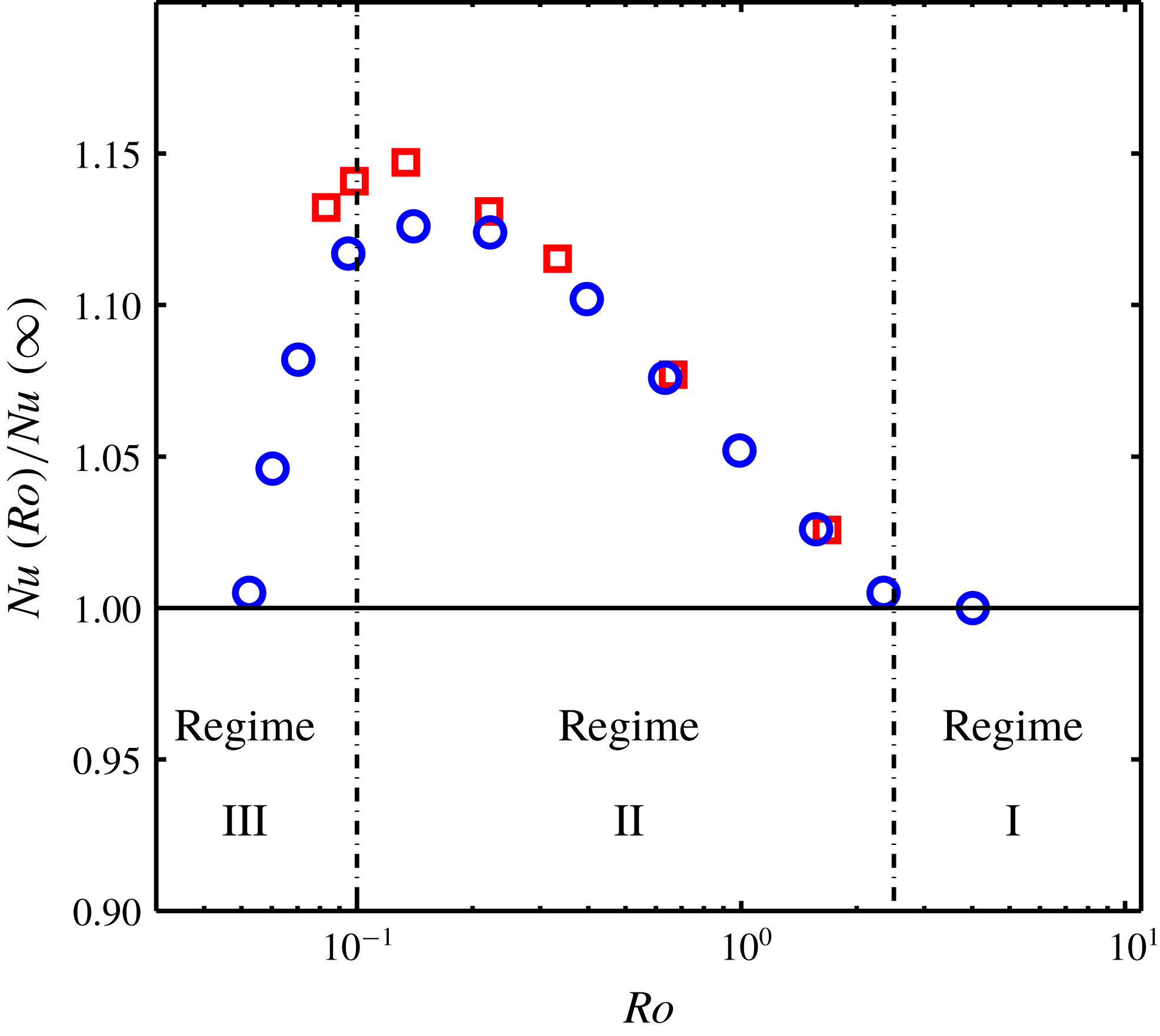
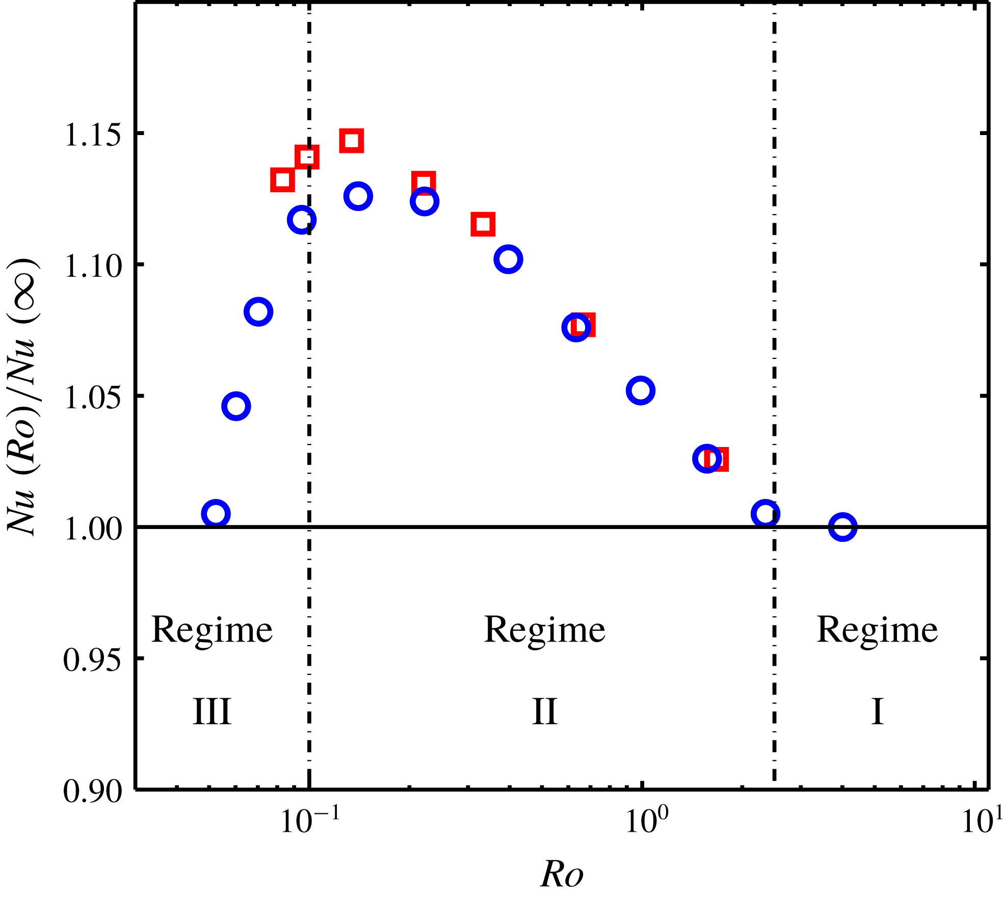
It is well known that the application of background rotation to Rayleigh–Bénard convection (RBC) leads to a significant flow departure from its non-rotating state. Three different regimes can be considered: (I) the rotation-unaffected regime (the flow is characterized by a so-called large-scale circulation (LSC), composed of tiny mushroom-shape plumes, and the heat flux remains constant), (II) the rotation-affected regime (rotation-aligned vortical plumes are the main features of the flow and the heat flux increases with increasing background rotation) and (III) the rotation-dominated regime (or geostrophic regime, the flow is turbulent but at the same time dominated by the Coriolis force; the heat flux drops dramatically with increasing background rotation). We refer to these regimes as regimes I, II and III, respectively. These different regimes are plotted in figure 1. In this figure and its caption,
 $Ra=\unicode[STIX]{x1D6FC}g\unicode[STIX]{x0394}TH^{3}/(\unicode[STIX]{x1D705}\unicode[STIX]{x1D708})$
is the Rayleigh number,
 $Pr=\unicode[STIX]{x1D708}/\unicode[STIX]{x1D705}$
is the Prandtl number,
 $Ro=\sqrt{\unicode[STIX]{x1D6FC}g\unicode[STIX]{x0394}T/H}/(2\unicode[STIX]{x1D6FA})$
is the Rossby number,
 $\unicode[STIX]{x1D6E4}=D/H$
is the aspect ratio and
 $Nu=qH/k\unicode[STIX]{x0394}T$
is the Nusselt number. In these dimensionless numbers
 $g$
is the gravitational acceleration,
 $H$
is the cell height,
 $\unicode[STIX]{x0394}T$
is the applied temperature difference,
 $\unicode[STIX]{x1D6FA}$
is the rotation rate,
 $D$
is the cell diameter,
 $q$
is the mean heat-current density and
 $k$
,
 $\unicode[STIX]{x1D6FC}$
,
 $\unicode[STIX]{x1D708}$
and
 $\unicode[STIX]{x1D705}$
are the thermal conductivity, the thermal expansion coefficient, kinematic viscosity and thermal diffusivity of the fluid, respectively. The transition between regimes I and II is strongly dependent on the aspect ratio and to a lesser extent on
 $Pr$
: for
 $\unicode[STIX]{x1D6E4}=1$
and
 $Pr=4.38$
it happens at
 $Ro\cong 2.5$
(Weiss et al.
Reference Weiss, Stevens, Zhong, Clercx, Lohse and Ahlers2010; Zhong & Ahlers Reference Zhong and Ahlers2010). The transition between regimes II and III depends strongly on
 $Pr$
and
 $Ra$
: for similar parameter values to our experiments, it occurs in the vicinity of
 $Ro=0.1$
where
 $Nu(Ro)$
displays a peak value (data from Zhong et al.
Reference Zhong, Stevens, Clercx, Verzicco, Lohse and Ahlers2009; Joshi et al.
Reference Joshi, Rajaei, Kunnen and Clercx2016).
The normalized heat transfer as a function of
 $Ro$
on logarithmic scales. Red squares are data for
 $Ra=1.2\times 10^{9}$
,
 $Pr=6.41$
and
 $\unicode[STIX]{x1D6E4}=1$
taken from Zhong et al. (Reference Zhong, Stevens, Clercx, Verzicco, Lohse and Ahlers2009); blue circles are data for
 $Ra=1.43\times 10^{9}$
,
 $Pr=6.2$
and
 $\unicode[STIX]{x1D6E4}=1$
taken from Joshi et al. (Reference Joshi, Rajaei, Kunnen and Clercx2016). The vertical dashed lines represent the demarcation lines between different regimes.
Regimes I and II and the transition between them are easily accessible with experiments and numerical simulations, thus they are better understood. On the other hand, the geostrophic regime (regime III) and the transition to this regime are less explored. It is worth mentioning that the geostrophic regime is the most relevant regime for astrophysical and geophysical applications, thus it is of utmost importance to understand this regime. Approaching the geostrophic regime is difficult as it requires both high turbulence intensity and rotationally constrained flow. Nonetheless, few studies have decisively entered the geostrophic regime (Ecke & Niemela Reference Ecke and Niemela2014; Stellmach et al.
Reference Stellmach, Lischper, Julien, Vasil, Cheng, Ribeiro, King and Aurnou2014; Cheng et al.
Reference Cheng, Stellmach, Ribeiro, Grannan, King and Aurnou2015; Kunnen et al.
Reference Kunnen, Ostilla-Mónico, van der Poel, Verzicco and Lohse2016; Rajaei et al.
Reference Rajaei, Kunnen and Clercx2017). Other experiments (Rossby Reference Rossby1969; Zhong et al.
Reference Zhong, Ecke and Steinberg1993; Liu & Ecke Reference Liu and Ecke1997; King et al.
Reference King, Stellmach, Noir, Hansen and Aurnou2009; Liu & Ecke Reference Liu and Ecke2009; Zhong et al.
Reference Zhong, Stevens, Clercx, Verzicco, Lohse and Ahlers2009; Weiss et al.
Reference Weiss, Stevens, Zhong, Clercx, Lohse and Ahlers2010; Zhong & Ahlers Reference Zhong and Ahlers2010; Kunnen et al.
Reference Kunnen, Stevens, Overkamp, Sun, van Heijst and Clercx2011; Weiss & Ahlers Reference Weiss and Ahlers2011a
,Reference Weiss and Ahlers
b
) and direct numerical simulations (King et al.
Reference King, Stellmach, Noir, Hansen and Aurnou2009; Schmitz & Tilgner Reference Schmitz and Tilgner2009, Reference Schmitz and Tilgner2010; Zhong et al.
Reference Zhong, Stevens, Clercx, Verzicco, Lohse and Ahlers2009; Stevens et al.
Reference Stevens, Clercx and Lohse2010; Horn & Shishkina Reference Horn and Shishkina2015) reach regime III but they did not enter deep into this regime. In addition to the experiments and direct numerical simulations (DNS), Julien and coworkers (Sprague et al.
Reference Sprague, Julien, Knobloch and Werne2006; Julien et al.
Reference Julien, Knobloch, Rubio and Vasil2012a
,Reference Julien, Rubio, Grooms and Knobloch
b
; Rubio et al.
Reference Rubio, Julien, Knobloch and Weiss2014) derived a set of asymptotically reduced equations in the limit
 $Ro\rightarrow 0$
, with
 $Ro$
the Rossby number denoting the ratio of the inertial and Coriolis forces. The experimental (Rajaei et al.
Reference Rajaei, Kunnen and Clercx2017) and DNS (Stellmach et al.
Reference Stellmach, Lischper, Julien, Vasil, Cheng, Ribeiro, King and Aurnou2014) studies show that these equations are indeed appropriate to study the geostrophic regime of rapidly rotating convection.
As a result of difficulties to explore regime III, our understanding of this regime and the transition to this regime is still limited. Nonetheless, two main mechanisms are proposed for this transition, by King et al. (Reference King, Stellmach, Noir, Hansen and Aurnou2009, Reference King, Stellmach and Aurnou2012) and Julien et al. (Reference Julien, Knobloch, Rubio and Vasil2012a
). King et al. (Reference King, Stellmach, Noir, Hansen and Aurnou2009, Reference King, Stellmach and Aurnou2012) suggested that the transition depends on the relative thicknesses of the viscous (
 $\unicode[STIX]{x1D6FF}_{u}$
) and thermal (
 $\unicode[STIX]{x1D6FF}_{T}$
) boundary layers. They showed that
 $\unicode[STIX]{x1D6FF}_{T}<\unicode[STIX]{x1D6FF}_{u}$
in regime II, while
 $\unicode[STIX]{x1D6FF}_{T}>\unicode[STIX]{x1D6FF}_{u}$
in regime III, within their range of parameter values. Therefore, they hypothesized that the transition between regimes II and III occurs when the viscous and thermal boundary layer (BL) thicknesses become approximately equal,
 $\unicode[STIX]{x1D6FF}_{u}\simeq \unicode[STIX]{x1D6FF}_{T}$
. However, a similar transition is also observed from numerical simulations with stress-free boundary conditions and no Ekman layers (Schmitz & Tilgner Reference Schmitz and Tilgner2009). On the other hand, Julien et al. (Reference Julien, Knobloch, Rubio and Vasil2012a
), using the asymptotically reduced equations, suggested that the transition occurs when the bulk is also rotation dominated and the vortical plumes span throughout the entire domain (columns): the vertical motion in the bulk is then suppressed, resulting in a drop in the heat transfer efficiency. Recently, Kunnen et al. (Reference Kunnen, Ostilla-Mónico, van der Poel, Verzicco and Lohse2016) also performed simulations with stress-free and no-slip boundary conditions showing that the transition does not always coincide with the intersection of the viscous and thermal boundary layer thicknesses, in contrast with King’s hypothesis. The study of Kunnen et al. supports more the point of view by Julien et al. rather than King’s, however, no certain conclusion can be drawn yet (Kunnen et al.
Reference Kunnen, Ostilla-Mónico, van der Poel, Verzicco and Lohse2016).
Up to now, the transition to regime III has thus been evaluated through various parameters. King et al. (Reference King, Stellmach, Noir, Hansen and Aurnou2009, Reference King, Stellmach and Aurnou2012) focused on the relative thicknesses of the Ekman and thermal BLs and global heat transfer, measured by laboratory experiments and numerical simulations. Julien et al. (Reference Julien, Knobloch, Rubio and Vasil2012a ) examined the vertical velocity and temperature fluctuations by simulations of asymptotically reduced equations. Kunnen et al. (Reference Kunnen, Ostilla-Mónico, van der Poel, Verzicco and Lohse2016) evaluated the thermal and Ekman BL thicknesses, heat transfer efficiency, distribution of dissipation and mean temperature gradients throughout the domain by DNS with no-slip and stress-free boundary conditions. However, the correct diagnostic parameter is not identified yet.
In this paper, we examine regimes II and III and the transition between them from a new perspective: the experimentally obtained Lagrangian velocity and acceleration fluctuations and autocorrelations. The results in regime I are also included, wherever appropriate, in order to have a comprehensive discussion. We also make the connection with the previous hypotheses when possible. The presented Lagrangian data allow us to examine the flow structures in all three regimes. Furthermore, it opens up new understanding of the physics behind all three regimes, in particular on the rotation-dominated regime and the transition to this regime.
We start with the experimental and numerical parameters used in this investigation in § 2. Next, the Lagrangian velocity root-mean-square (r.m.s.) values and autocorrelations are discussed in §§ 3 and 4, respectively. In § 5 the acceleration r.m.s. values are presented and discussed. In § 6 the inertial wave, observed in the velocity and acceleration autocorrelations, is discussed. We summarize our main findings in § 7.
2 Methods and parameters
Experiments have been performed using the experimental set-up described in detail in Rajaei et al. (Reference Rajaei, Joshi, Alards, Kunnen, Toschi and Clercx2016a ,Reference Rajaei, Joshi, Kunnen and Clercx b , Reference Rajaei, Kunnen and Clercx2017), Rajaei (Reference Rajaei2017). Here we briefly discuss the main features of the set-up. The experimental set-up is composed of a cylindrical convection cell and a tracking system. In the following paragraphs, we will first explain the convection cell. Then, the tracking system and post-processing of the data are explained.
The cylindrical convection cell, filled with water, is the same as the one used in Rajaei et al. (Reference Rajaei, Joshi, Alards, Kunnen, Toschi and Clercx2016a
,Reference Rajaei, Joshi, Kunnen and Clercx
b
, Reference Rajaei, Kunnen and Clercx2017). The convection cell is 200 mm tall with diameter of 200 mm, resulting in
 $\unicode[STIX]{x1D6E4}=1$
. A copper plate, connected to a resistance heater, is placed at the bottom. The copper temperature is measured by a thermistor positioned inside a hole at the centre of the copper plate. A cooling chamber seals the cell from above. The coolant and the fluid inside the cell are separated by a thin sapphire plate. The cooling chamber and the copper plate are connected by a Plexiglas cylindrical vessel. In order to avoid the distortion of the illumination from the side, the cylindrical vessel is placed inside a Plexiglas cubic box.
The three-dimensional particle tracking velocimetry (3D-PTV) system used in this study consists of four charge-coupled device (CCD) cameras (MegaPlus ES2020,
 $1600\times 1200$
pixels) positioned above the convection cell. The cameras record the flow field at a frequency of
 $30~\text{Hz}$
which is adequate to resolve the smallest length and time scales of the flow field. The illumination is provided by four arrays of light-emitting diodes (LEDs). The tracer particles are fluorescent polyethylene particles (supplied by Cospheric Co., USA) and have a mean density of
 $1002~\text{kg}~\text{m}^{-3}$
and a diameter of
 $75{-}90~\unicode[STIX]{x03BC}\text{m}$
. In the current study, we use a particle tracking system based on the system developed at ETH Zürich (Switzerland) (Maas, Gruen & Papantoniou Reference Maas, Gruen and Papantoniou1993; Malik, Dracos & Papantoniou Reference Malik, Dracos and Papantoniou1993; Willneff Reference Willneff2002, Reference Willneff2003; Lüthi, Tsinober & Kinzelbach Reference Lüthi, Tsinober and Kinzelbach2005). All experimental equipment, including the convection cell and the 3D-PTV system, is placed on the rotating table.
The 3D-PTV experiments are performed in two different fashions: high particle concentration (HPC) and low particle concentration (LPC). Depending on the parameters of interest, either HPC or LPC data sets are used. Note that HPC experiments consist of more trajectories at each time step (more data points in space at each time step) but the trajectories are shorter compared to the LPC experiments. The LPC experiments are used for the calculations of root-mean-square values and autocorrelations of the velocity and acceleration. The HPC experiments are only used for the vortex detection technique and the subsequent analysis in § 4.1. In LPC experiments, an average number of
 ${\sim}500$
randomly distributed particles are tracked at each time step. On the other hand, in the HPC experiments, an average number of
 ${\sim}1600$
(
 ${\sim}2700$
) randomly distributed particles are tracked at each time step in the cell centre (close to the top plate).
The experiments are performed at constant
 $Ra=1.3\times 10^{9}$
,
 $Pr=6.7$
and
 $\unicode[STIX]{x1D6E4}=1$
while
 $Ro$
varies between
 $0.041$
and
 $\infty$
(
 $\unicode[STIX]{x1D6FA}$
between
 $4.12~\text{rad}~\text{s}^{-1}$
and
 $0$
). We analyse the Lagrangian velocity/acceleration root-mean-square (r.m.s.) values and autocorrelations. The Lagrangian velocity and acceleration r.m.s. values are calculated in the volumes at three different regions, vertically separated and centred at the rotation axis. Region I (centre) covers the height
 $0.375H<z<0.625H$
with a volume of
 $50\times 50\times 50~\text{mm}^{3}$
, region II (
 $z=0.8H$
) covers the height
 $0.75H<z<0.85H$
with a volume of
 $50\times 50\times 20~\text{mm}^{3}$
and region III (
 $z=0.975H$
) covers the height
 $0.95H<z<H$
with a volume of
 $50\times 50\times 10~\text{mm}^{3}$
. However, the Lagrangian velocity and acceleration autocorrelations are calculated based on the data collected in a volume of approximately
 $80\times 60\times 50~\text{mm}^{3}(x,y,z)$
for both the centre (covering a volume between
 $z=0.375H$
and
 $z=0.625H$
) and close to the top plate (
 $z=0.875H$
; covering a volume between
 $z=0.75H$
and
 $z=H$
). Note that it is not possible to divide the measurement domain into smaller subvolumes for the Lagrangian autocorrelations since the particles do not reside in a thin layer of fluid for a long time.
3 Lagrangian r.m.s. velocity
We start with the presentation of the Lagrangian velocity fluctuations at the
 $z=0.5H$
(centre), at
 $z=0.8H$
and at
 $z=0.975H$
. We focus on regimes II and III in rotating RBC and how the velocity fluctuations can contribute to our understanding of these regimes and the transition between them.
In Rajaei et al. (Reference Rajaei, Joshi, Kunnen and Clercx2016b
), an (an)isotropy ratio based on the velocity fluctuations has been introduced to treat the large-scale isotropy,
 $RU=u_{z}^{rms}/u_{xy}^{rms}$
. Note that the statistics in
 $x$
and
 $y$
directions are almost the same, i.e.
 $u_{xy}^{rms}=(u_{x}^{rms}+u_{y}^{rms})/2\approx u_{x}^{rms}\approx u_{y}^{rms}$
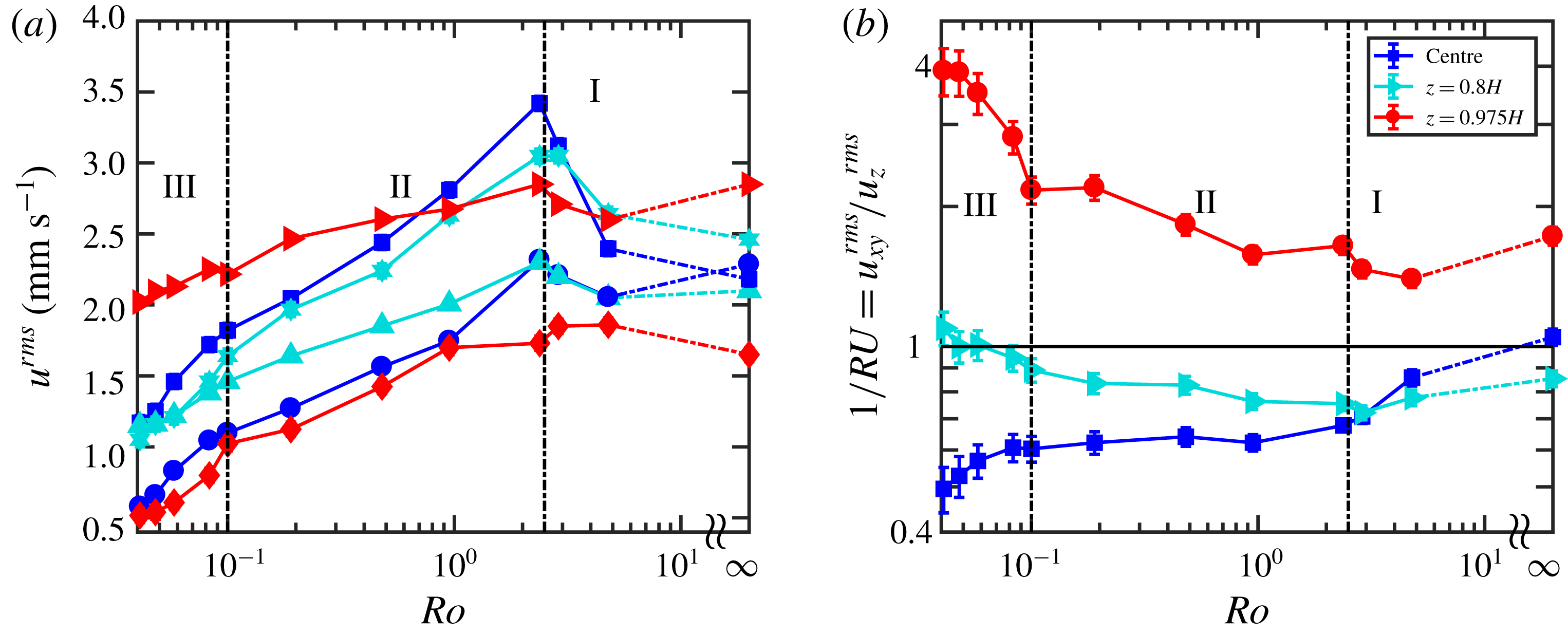
. Figure 2(a,b) shows the velocity fluctuations and the inverse of the anisotropy ratio,
 $1/RU=u_{xy}^{rms}/u_{z}^{rms}$
, as a function of
 $Ro$
for three measurement sets for regimes II and III. We plot
 $1/RU$
instead of
 $RU$
as it shows the trends more clearly. Regimes I and II of these graphs have been treated in Rajaei et al. (Reference Rajaei, Joshi, Kunnen and Clercx2016b
). Here, we limit our discussion mainly to regime III.
The measurements at the cell centre, dark blue symbols in figure 2(a), show that the horizontal and vertical velocity fluctuations continue to decrease in regime III with decreasing
 $Ro$
, but at faster decay rates. The decay in regimes II and III is a result of the turbulence suppression with increase in background rotation (Chandrasekhar Reference Chandrasekhar1961). The large-scale anisotropy becomes even larger with decreasing
 $Ro$
in regime III, see blue squares in figure 2(b). The horizontal and vertical r.m.s. velocities at the cell centre decrease at a similar rate. However, the ratio
 $1/RU$
decreases with decreasing
 $Ro$
because
 $u_{xy}^{rms}$
is smaller than
 $u_{z}^{rms}$
. Similar to the results at the centre, at
 $z=0.8H$
(cyan symbols) the vertical velocity fluctuation decreases with decreasing
 $Ro$
due to the turbulence suppression with increase in background rotation. The horizontal component decreases as well, but reduction of the vertical component is stronger than that of the horizontal one. The horizontal velocity fluctuation is governed by two contributing factors: decrease due to turbulence reduction with background rotation and enhancement due to swirling motions, contributed by the vortical plumes in the horizontal plane. Therefore, the horizontal velocity fluctuation decreases at a slower rate than the vertical counterpart. The horizontal and vertical components intersect in regime III:
 $1/RU$
goes from below one to values slightly above one. At
 $z=0.975H$
, both horizontal and vertical velocity fluctuations decrease with decreasing
 $Ro$
. However, as explained for
 $z=0.8H$
, the vertical velocity fluctuation reduces faster compared to its horizontal counterpart due to the enhancement of the horizontal velocities by the vortical plumes. This results in an increase in the ratio
 $1/RU$
with decreasing
 $Ro$
, as is clear from figure 2(b).
(a) Horizontal and vertical velocity fluctuations from experiments. Blue circles and squares are the horizontal and vertical components at the cell centre, respectively. Cyan upright-pointing triangles and stars are the horizontal and vertical components at
 $z=0.8H$
, respectively. Red right-pointing triangles and diamonds are the horizontal and vertical components at
 $z=0.975H$
. The error bars are of the same size as the symbols. (b) The inverse of the anisotropy ratio
 $1/RU=u_{xy}^{rms}/u_{z}^{rms}$
.
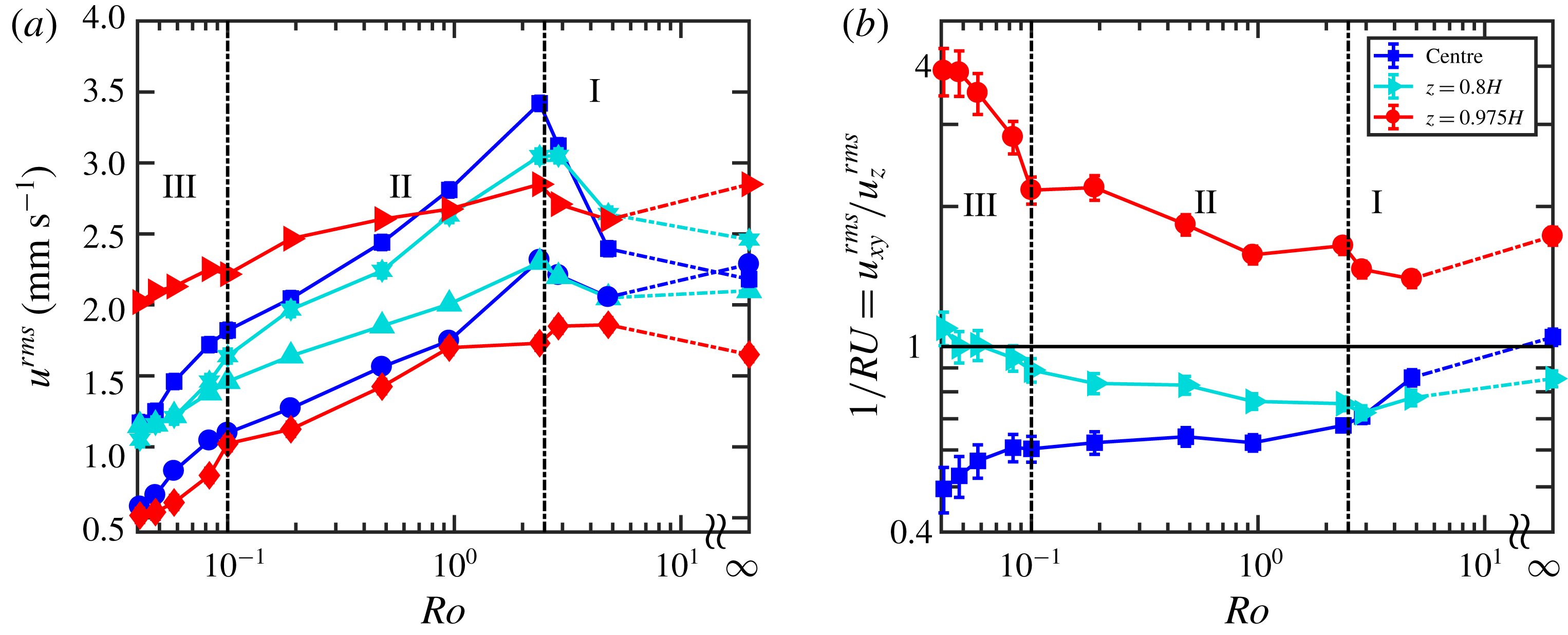
In conclusion, in regimes II and III, the horizontal velocity fluctuations at
 $z=0.975H$
and
 $z=0.8H$
decrease at a slower rate compared to their vertical counterparts due to the vortical plumes. In regime III, a faster decay is observed for the vertical component of the velocity throughout the convection cell. This observation supports the hypothesis proposed by Julien et al. (Reference Julien, Knobloch, Rubio and Vasil2012a
) stating that the strong suppression of the vertical motion results in a drop in heat transfer efficiency in regime III.
4 Lagrangian velocity autocorrelation
The Lagrangian velocity autocorrelation is one of the useful Lagrangian quantities which provides insight into the turbulent diffusivity of a fluid parcel (Taylor Reference Taylor1921). The Lagrangian velocity autocorrelation shows the time period over which the particle velocity remains correlated with the velocity at the previous times. It is expected that the particle velocity remains correlated for a longer time if the flow is coherent. Therefore, the Lagrangian velocity autocorrelation can be used as a measure of flow coherence as well. The Lagrangian velocity autocorrelation is defined as
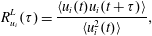 $$\begin{eqnarray}R_{u_{i}}^{L}(\unicode[STIX]{x1D70F})=\frac{\langle u_{i}(t)u_{i}(t+\unicode[STIX]{x1D70F})\rangle }{\langle u_{i}^{2}(t)\rangle },\end{eqnarray}$$
with
 $u_{i}$
the
 $i$
th component of the velocity signal,
 $\unicode[STIX]{x1D70F}$
the time lag and
 $\langle \cdots \rangle$
the ensemble average. Another useful parameter in the evaluation of the coherent structures in turbulent flows is the integral time scale, defined as
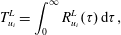 $$\begin{eqnarray}T_{u_{i}}^{L}=\int _{0}^{\infty }R_{u_{i}}^{L}(\unicode[STIX]{x1D70F})\,\text{d}\unicode[STIX]{x1D70F},\end{eqnarray}$$
which is a measure for the time a fluid parcel velocity remains correlated providing insight into the large-scale flow coherence.
In the present study the residence time of the particles in the observation domain (estimated as
 $d_{obs}/u^{rms}$
where
 $d_{obs}$
is the length/width/depth of the observation volume and
 $u^{rms}$
is the velocity r.m.s.) is
 ${\sim}25\unicode[STIX]{x1D70F}_{\unicode[STIX]{x1D702}}$
, while the autocorrelation coefficient drops below 0.1 at approximately
 $15\unicode[STIX]{x1D70F}_{\unicode[STIX]{x1D702}}$
(see figure 3) for most of the rotation rates. Furthermore, as an a posteriori check
 $d_{obs}$
for the length and width is at least 5 times larger than
 $V_{drift}T^{L}$
, where
 $V_{drift}$
is the horizontal velocity of the vortical columns; see Rajaei et al. (Reference Rajaei, Kunnen and Clercx2017) for the calculation of
 $V_{drift}$
. They indicate that the bias error induced by the limited volume is small.
For large time lags
 $\unicode[STIX]{x1D70F}$
the autocorrelation values are not perfectly converged due to the shortage of long trajectories. Lack of convergence leads to larger errors in the calculation of the integral time scale. Therefore, we fit an exponential function over the time period for which the velocity autocorrelation shows a clear exponential decay. Exponential fitting is chosen since in homogeneous isotropic turbulence (HIT) the velocity decorrelation at large
 $\unicode[STIX]{x1D70F}$
is expected to be exponential (Mordant et al.
Reference Mordant, Metz, Michel and Pinton2001; Mordant, Crawford & Bodenschatz Reference Mordant, Crawford and Bodenschatz2004a
; Gervais, Baudet & Gagne Reference Gervais, Baudet and Gagne2007; Del Castello & Clercx Reference Del Castello and Clercx2011); it plays a crucial role in some dispersion models (Sawford Reference Sawford1991). The linear–logarithmic plots (not shown here) confirm the exponential decay of the velocity autocorrelation at large
 $\unicode[STIX]{x1D70F}$
. Note that at very small (dissipative scale)
 $\unicode[STIX]{x1D70F}$
, in our experiments
 $\unicode[STIX]{x1D70F}\lesssim 1$
s, the velocity autocorrelation shows non-exponential behaviour (the curvature of the velocity autocovariance at
 $\unicode[STIX]{x1D70F}=0$
is equal to the acceleration variance) (Sawford Reference Sawford1991; Voth et al.
Reference Voth, La Porta, Crawford, Alexander and Bodenschatz2002; Mordant, Lévêque & Pinton Reference Mordant, Lévêque and Pinton2004b
). The integral time scale is calculated using a combination of the actual velocity autocorrelation curve for small time lags and the exponentially fitted curve for large time lags. The integral time scale can also be estimated through the aforementioned exponential fitted curve
 $\text{e}^{-\unicode[STIX]{x1D70F}/\unicode[STIX]{x1D70F}_{0}}$
, where
 $\unicode[STIX]{x1D70F}_{0}$
is the integral time scale. However, the latter approach neglects the non-exponential decay for small time lags, so small differences are expected. We shall use the first method (i.e. a combination of the actual velocity autocorrelation curve for small time lags and the exponentially fitted curve for large time lags) unless otherwise stated.
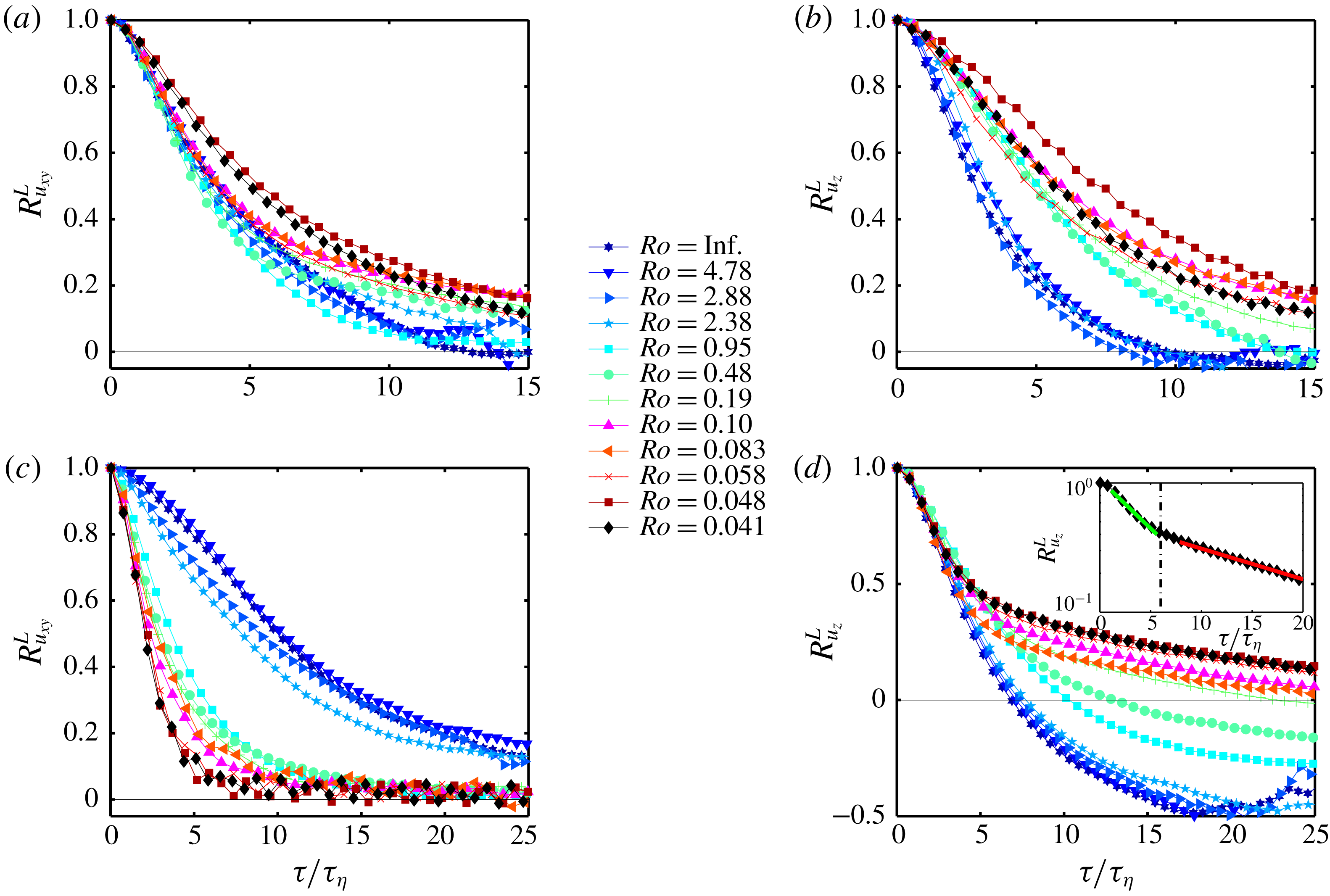
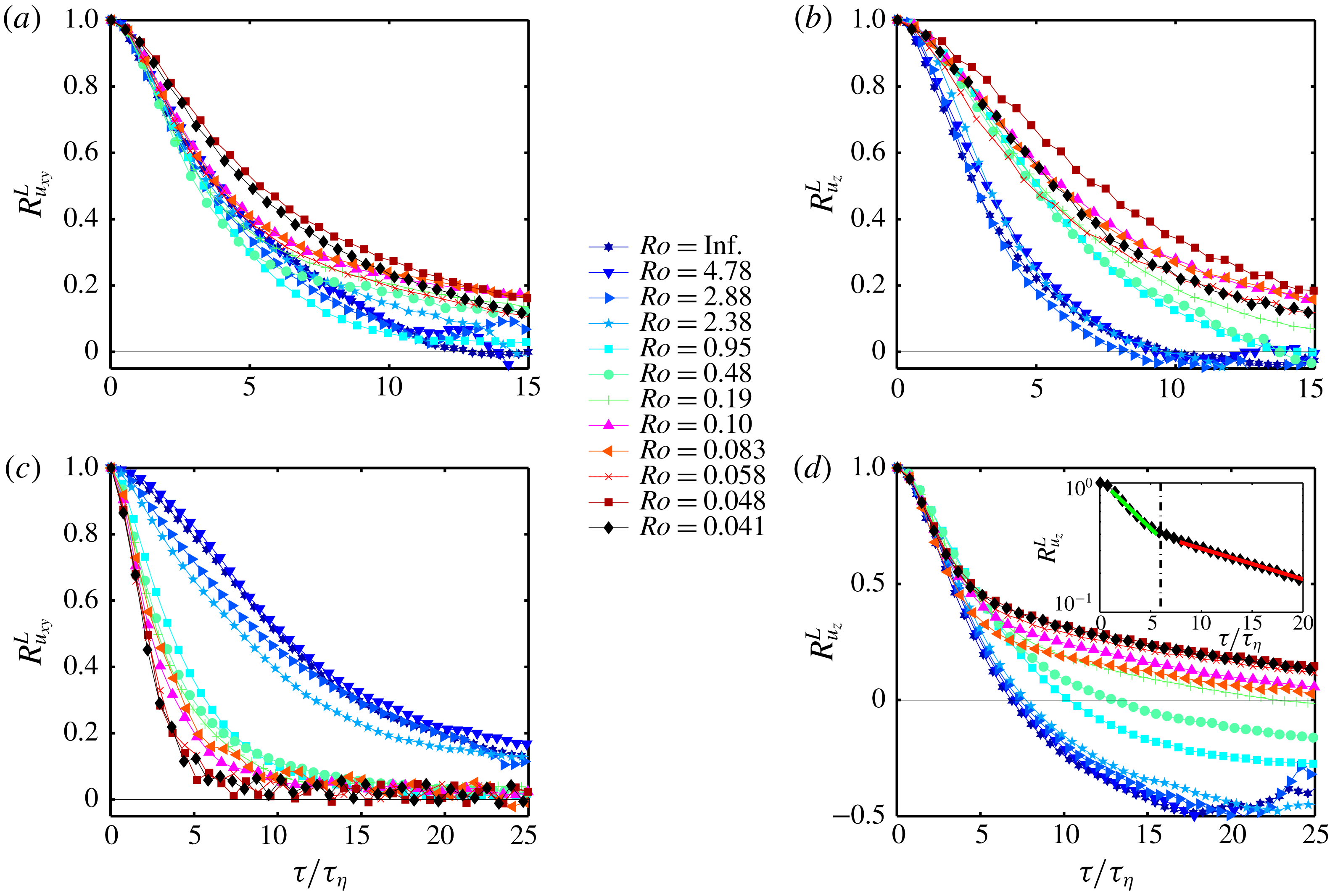
(a) Horizontal and (b) vertical Lagrangian velocity autocorrelations at the centre and (c) horizontal and (d) vertical Lagrangian velocity autocorrelations close to the top as a function of
 $Ro$
. The inset in (d) is the vertical velocity autocorrelation for
 $Ro=0.041$
at
 $z=0.875H$
. The green and red lines are the exponential fits, proportional to
 $\text{e}^{-\unicode[STIX]{x1D70F}/\unicode[STIX]{x1D70F}_{0}}$
with
 $\unicode[STIX]{x1D70F}_{0}=\unicode[STIX]{x1D70F}_{1}$
for
 $1\lesssim \unicode[STIX]{x1D70F}/\unicode[STIX]{x1D70F}_{\unicode[STIX]{x1D702}}\lesssim 6$
and
 $\unicode[STIX]{x1D70F}_{0}=\unicode[STIX]{x1D70F}_{2}$
for
 $\unicode[STIX]{x1D70F}/\unicode[STIX]{x1D70F}_{\unicode[STIX]{x1D702}}\gtrsim 6$
, respectively. The dash-dotted black line is located at
 $\unicode[STIX]{x1D70F}/\unicode[STIX]{x1D70F}_{\unicode[STIX]{x1D702}}=6$
.
Kolmogorov time scale,
 $\unicode[STIX]{x1D70F}_{\unicode[STIX]{x1D702}}$
(in seconds), as a function of
 $Ro$
for the measurements at the cell centre and close to the top plate. The dissipation rates are calculated from DNS data (Rajaei et al.
Reference Rajaei, Joshi, Kunnen and Clercx2016b
). The dissipation rates from DNS are for slightly different
 $Ro$
numbers, but we expect that they are still representative for the current experiments given the weak
 $Ro$
-dependence displayed here.

We start with the data at the centre. Figure 3(a,b) shows the autocorrelation of the velocity in the
 $xy$
and
 $z$
directions at the cell centre, respectively. The time lag is non-dimensionalized by the local Kolmogorov time scale, given in table 1 calculated from direct numerical simulations using the same parameter settings, see Alards et al. (Reference Alards, Rajaei, Del Castello, Kunnen, Toschi and Clercx2017) and Rajaei (Reference Rajaei2017) for the details of the numerical method. Note that the Kolmogorov time scale differs depending on the position within the cylinder. In table 1, we also report the Froude number; a measure for the importance of the centrifugal buoyancy and defined as
 $Fr=\unicode[STIX]{x1D6FA}^{2}R/g$
where
 $R$
is the cell radius. It is worth mentioning that Horn & Aurnou (Reference Horn and Aurnou2018) suggest that centrifugal effects are not important when
 $Fr<R/H$
(in our case
 $R/H=0.5$
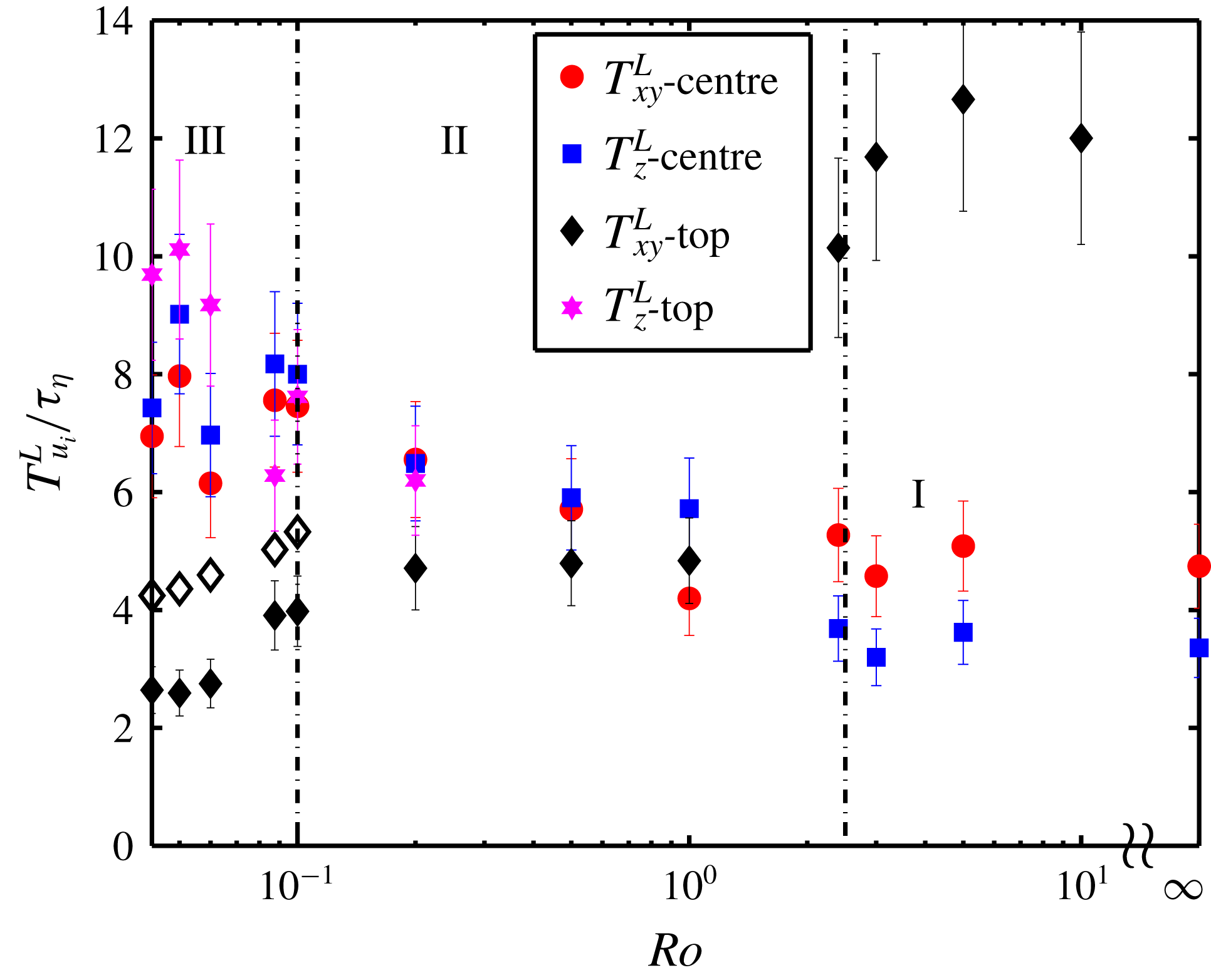
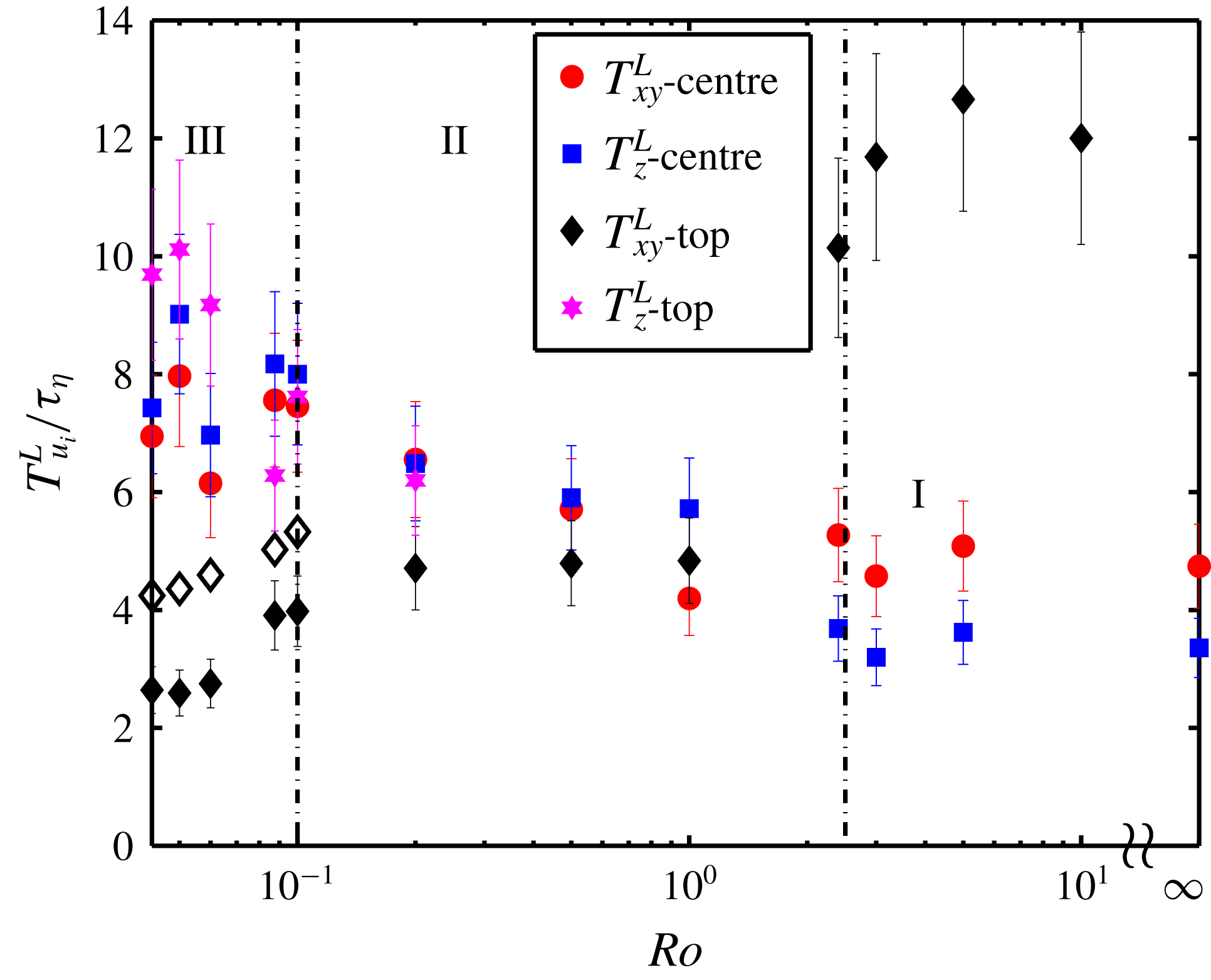
). The velocity autocorrelations in regime I collapse for both horizontal and vertical components. Figure 4 displays the Lagrangian integral time scales, non-dimensionalized by the local Kolmogorov time scale, at the cell centre and at
 $z=0.875H$
. The horizontal and vertical integral time scales at the cell centre, red circles and blue squares, remain almost constant in regime I as well. As mentioned before, the integral time scale is a measure of the large-scale coherence. Therefore, one expects smaller integral time scales at
 $Ro\simeq 2.4$
, where the LSC breaks down and the flow lacks a dominant large-scale coherent structure. However, figure 4 does not show a decrease around
 $Ro\simeq 2.4$
. It can be explained by the fact that the LSC is best visible near the top/bottom and side boundaries: the large-scale flow at the cell centre is close to HIT (Sun, Zhou & Xia Reference Sun, Zhou and Xia2006; Rajaei et al.
Reference Rajaei, Joshi, Kunnen and Clercx2016b
) and there is no clear signature of the large-scale coherent structure in the cell centre for
 $Ro\gg 1$
. In regime II, the horizontal and vertical velocity autocorrelations progressively increase with reduction of
 $Ro$
, see figure 3(a,b). These enhancements are also reflected in the integral time scales, see red circles and blue squares in figure 4. In regime II, the vortical plumes are already present as the large-scale flow features, resulting in an enhancement of the large-scale coherence. Note that, in contrast to the LSC, the vortical plumes are visible in the large-scale flow in the centre (Rajaei et al.
Reference Rajaei, Joshi, Kunnen and Clercx2016b
). In regime III, the vortical plumes form columns and the vertical and horizontal velocity autocorrelations show non-monotonic trends with respect to
 $Ro$
but only reveal little changes in this regime. The horizontal and vertical integral time scales also show non-monotonic behaviours. However, the non-monotonic trends are within the error bars.
Integral time scale as a function of
 $Ro$
for measurements both at the cell centre and top (
 $z=0.875H$
). The error is estimated by calculating the integral time scale for different segments of the experimental data. The error is approximately
 $15\,\%$
. The open diamonds are estimates of the corresponding filled diamonds, see the text for details.
We continue with the data at
 $z=0.875H$
. Figure 3(c,d) shows the velocity autocorrelations at
 $z=0.875H$
for the
 $xy$
and
 $z$
directions, respectively. The inset of figure 3(d) shows
 $R_{u_{z}}^{L}$
for
 $Ro=0.041$
with the horizontal axis in logarithmic scale. The flow shows strong horizontal correlation in regime I. The horizontal velocity autocorrelations remain correlated for a long time due to the LSC which is prominently present at this location, see also the black diamonds in figure 4. As the LSC vanishes for
 $Ro\lesssim 2.4$
, the horizontal velocity correlation time drops abruptly, see also the black diamonds in figure 4. The horizontal velocity correlation time at
 $z=0.875H$
(black diamonds) in regime II are approximately equal to the horizontal velocity correlation time at the centre (red circles) in regime I, where the LSC is not felt either. As the LSC has vanished, the mean horizontal velocity becomes zero, thus no contribution from the mean velocity is expected in the correlations in regime II. Note that, in contrast to the velocity r.m.s. values, the autocorrelation data are calculated for the total velocity signal for
 $Ro\gtrsim 2.4$
at
 $z=0.875H$
. For the rest of the data (data at the centre and data for
 $Ro\lesssim 2.4$
at
 $z=0.875H$
) the mean velocities are zero. In regime II (
 $2.4\lesssim Ro\lesssim 0.1$
), the horizontal correlation decreases slightly with decreasing
 $Ro$
. In regime III,
 $Ro\lesssim 0.1$
, the horizontal correlation decreases even further as
 $Ro$
goes down and its corresponding integral time scale (black diamonds) becomes as small as two times the Kolmogorov time scale (
 $T_{u_{xy}}^{L}/\unicode[STIX]{x1D70F}_{\unicode[STIX]{x1D702}}\sim 2$
). The decrease in the horizontal autocorrelation throughout regimes II and III can be explained by knowing that the swirling motion in the horizontal plane near the top plate results in a continuous change of velocity direction in this region. An estimate of the time scale of the decorrelation of the horizontal velocity autocorrelation, due to swirling motions near the top plate, can be calculated by using the horizontal velocity of the fluid parcel and the nominal radius of a vortical plume. If we assume that a fluid parcel follows perfectly a circular path,
 $u_{x}$
(or
 $u_{y}$
) decorrelates when a quarter of the circle circumference is covered. Therefore, an approximation of the decorrelation time is given by
 $\unicode[STIX]{x1D70F}_{h}=(\unicode[STIX]{x03C0}L_{c}/u_{h})/4$
where
 $u_{h}$
is the magnitude of the horizontal velocity,
 $u_{h}=(u_{x}^{2}+u_{y}^{2})^{1/2}$
, and
 $L_{c}$
is the so-called critical length,
 $L_{c}=4.8154Ek^{1/3}$
(Chandrasekhar Reference Chandrasekhar1961) with
 $Ek$
the Ekman number defined as
 $Ek=Ro\sqrt{Pr/Ra}$
. The
 $\unicode[STIX]{x1D70F}_{h}$
values are shown as open diamonds in figure 4 and they display similar trends as the measured integral time scales. Note that it is expected that the horizontal velocity autocorrelation is affected by the drift velocity of the vortical columns. However, quantifying that effect is rather elusive. One might expect that the integral time scale of the horizontal velocity at the centre follows the behaviour of its counterpart close to the top plate when
 $Ro$
is small. However, we know that the horizontal swirling velocity becomes smaller as we go down in the vortex column. Therefore,
 $u_{xy}$
decorrelates more rapidly (and
 $T_{u_{xy}}^{L}$
is smaller) close to the top than near the cell centre, given that we expect the horizontal structure size to be equal close to the top and at the cell centre.
In regime III, an oscillatory behaviour is observed in the horizontal component of the velocity near the top plate, see the tails of the correlations in figure 3(c). We will treat this intriguing oscillatory behaviour in detail in § 6 and show that not only Earth’s gravity determines the flow dynamics in our experiment but also Earth’s rotation.
The vertical velocity autocorrelations, figure 3(d), show no appreciable changes with rotation in regime I. As can be seen from the graph, they show persistent negative values. This is in agreement with our picture with an LSC present where a fluid parcel moves upward on one side and downward on the other side of the cell. Considering the general picture, one expects that the anti-correlation occurs at
 $0.5d_{obs}/u_{LSC}$
, where
 $d_{obs}$
is the length of the observation domain and
 $u_{LSC}$
is the fluid velocity in the LSC, calculated based on the LSC Reynolds number (Song & Tong Reference Song and Tong2010). The anti-correlation starts at
 $\unicode[STIX]{x1D70F}/\unicode[STIX]{x1D70F}_{\unicode[STIX]{x1D702}}\approx 7.0$
(
 $\unicode[STIX]{x1D70F}\approx 7.5~\text{s}$
), which is compatible with
 $0.5d_{obs}/u_{LSC}\approx 6~\text{s}$
. The vertical velocity autocorrelations collapse in regime I, with a rather large anti-correlation;
 $-0.5$
at
 $\unicode[STIX]{x1D70F}/\unicode[STIX]{x1D70F}_{\unicode[STIX]{x1D702}}=25$
. The LSC vanishes for
 $Ro\lesssim 2.4$
, and the vertical velocity anti-correlation gradually diminishes. For relatively high rotation rates,
 $Ro\lesssim 0.5$
, the anti-correlation in the vertical velocity autocorrelation disappears.
The vertical integral time scales in regime I and part of regime II at
 $z=0.875H$
are not reported due to the negative values in the vertical velocity autocorrelations. The vertical integral time scales in regimes II and III (pink stars in figure 4) increase with decreasing
 $Ro$
which is an indication of enhancement in the flow coherence, which we expect to be due to a stronger vertical coherence of the vortical plumes.
4.1 Small Ro: emergence of two time scales
As mentioned before, an exponential decay at large time lags in the velocity autocorrelation is expected; it plays a crucial role in Sawford’s stochastic dispersion model (Sawford Reference Sawford1991). Our experimental data also confirm the exponential decay, proportional to
 $\text{e}^{-\unicode[STIX]{x1D70F}/\unicode[STIX]{x1D70F}_{0}}$
, in the velocity autocorrelation. As mentioned before, the behaviour of the velocity autocorrelation is far from an exponential decay at the dissipative time lags
 $\unicode[STIX]{x1D70F}/\unicode[STIX]{x1D70F}_{\unicode[STIX]{x1D702}}\lesssim 1$
(Sawford Reference Sawford1991; Voth et al.
Reference Voth, La Porta, Crawford, Alexander and Bodenschatz2002; Mordant et al.
Reference Mordant, Lévêque and Pinton2004b
). However, here we focus on the large time lags
 $\unicode[STIX]{x1D70F}/\unicode[STIX]{x1D70F}_{\unicode[STIX]{x1D702}}\gtrsim 1$
of the velocity autocorrelations.
For all rotation rates at the cell centre and most of the rotation rates at
 $z=0.875H$
, the slope of the exponential decay is constant for
 $\unicode[STIX]{x1D70F}/\unicode[STIX]{x1D70F}_{\unicode[STIX]{x1D702}}\gtrsim 1$
, i.e. a single decay constant
 $\unicode[STIX]{x1D70F}_{0}$
in the expression
 $\text{e}^{-\unicode[STIX]{x1D70F}/\unicode[STIX]{x1D70F}_{0}}$
is observed. However, for the vertical velocity autocorrelation for
 $Ro\lesssim 0.19$
at
 $z=0.875H$
a second time scale emerges. The inset of figure 3(d) shows the vertical velocity autocorrelation for
 $Ro=0.041$
on a logarithmic scale. The green and red lines are exponential fits, proportional to
 $\text{e}^{-\unicode[STIX]{x1D70F}/\unicode[STIX]{x1D70F}_{i}}$
, fitted to the part where the autocorrelation shows a clear exponential decay. As can be seen, there exist two time scales
 $\unicode[STIX]{x1D70F}_{i}$
;
 $\unicode[STIX]{x1D70F}_{1}$
for small time lags (
 $1\lesssim \unicode[STIX]{x1D70F}/\unicode[STIX]{x1D70F}_{\unicode[STIX]{x1D702}}\lesssim 6$
) and
 $\unicode[STIX]{x1D70F}_{2}$
for large time lags (
 $\unicode[STIX]{x1D70F}/\unicode[STIX]{x1D70F}_{\unicode[STIX]{x1D702}}\gtrsim 6$
). The dash-dotted black line is at
 $\unicode[STIX]{x1D70F}=6~\text{s}$
, where the change in slope occurs.
We can calculate the two correlation time scales (
 $\unicode[STIX]{x1D70F}_{1}$
and
 $\unicode[STIX]{x1D70F}_{2}$
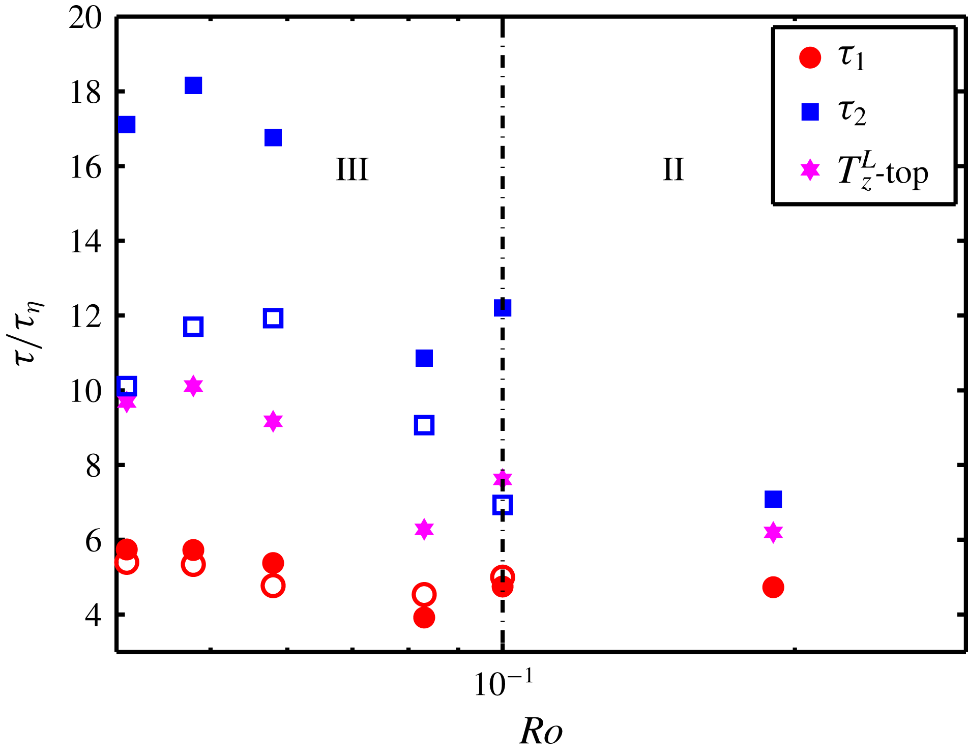
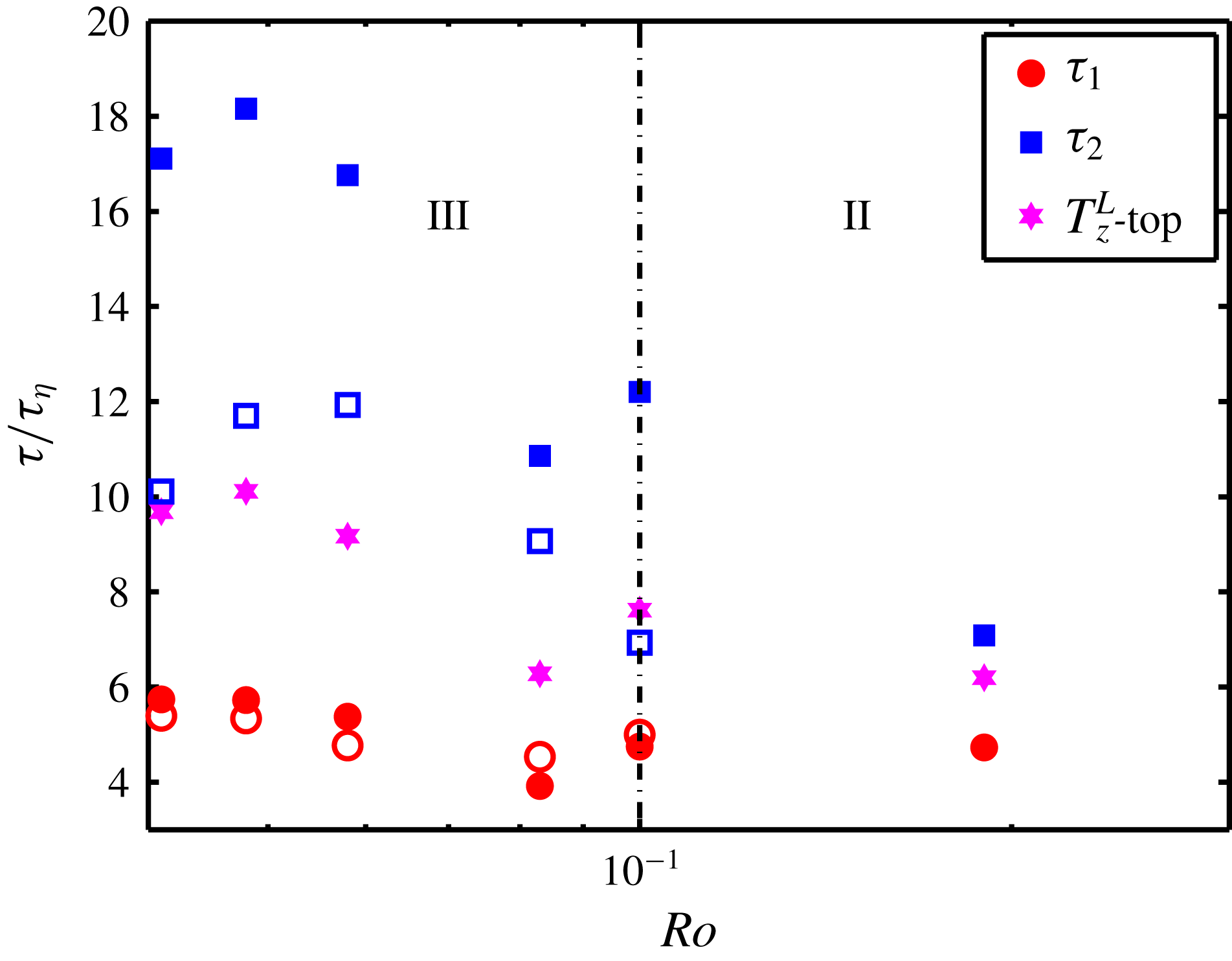
) for the vertical velocity autocorrelations plotted in figure 3(d). The results are plotted in figure 5 (solid symbols) as a function of
 $Ro$
. The smaller correlation time scales (
 $\unicode[STIX]{x1D70F}_{1}$
), present for smaller
 $\unicode[STIX]{x1D70F}$
and represented by the solid red circles, remain almost unchanged in the regimes II and III while the larger correlation time scales (
 $\unicode[STIX]{x1D70F}_{2}$
), present for larger
 $\unicode[STIX]{x1D70F}$
and represented by solid blue squares, increase with decreasing
 $Ro$
. The pink stars are the vertical integral time scales, taken from figure 4. As expected, they fall between the solid squares and circles. The open symbols will be discussed later.
Two correlation time scales as a function of
 $Ro$
. The small and large time scales are represented by
 $\unicode[STIX]{x1D70F}_{1}$
and
 $\unicode[STIX]{x1D70F}_{2}$
, respectively. The solid squares and circles represent the correlation time scales calculated based on the data in figure 3(d). The open symbols are the correlation time scales calculated based on the
 $Q$
-criterion method. Pink stars are the vertical integral time scales at
 $z=0.875H$
, taken from figure 4. The error is approximately 30 % for the open symbols and 15 % for the solid symbols.
In order to study the origin of the two correlation time scales, the flow domain is divided into plume and non-plume regions. The so-called
 $Q$
-criterion (Hunt, Wray & Moin Reference Hunt, Wray and Moin1988) is a widely used method for vortex detection. We apply the
 $Q$
-criterion for a three-dimensional flow field: a vortex is defined as a spatial region where
 $$\begin{eqnarray}Q={\textstyle \frac{1}{2}}(\Vert \overline{\overline{\unicode[STIX]{x1D734}}}\Vert ^{2}-\Vert \overline{\overline{\unicode[STIX]{x1D64E}}}\Vert ^{2})>0,\end{eqnarray}$$
where
 $\overline{\overline{\unicode[STIX]{x1D734}}}$
and
 $\overline{\overline{\unicode[STIX]{x1D64E}}}$
are the antisymmetric and symmetric parts of the velocity gradient tensor, respectively. The operator
 $\Vert \cdots \Vert$
represents the Euclidean norm defined as
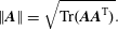 $$\begin{eqnarray}\Vert \boldsymbol{A}\Vert =\sqrt{\text{Tr}(\boldsymbol{A}\boldsymbol{ A}^{\text{T}})}.\end{eqnarray}$$
We have previously applied the
 $Q$
-criterion method on 3D-PTV data (Rajaei et al.
Reference Rajaei, Kunnen and Clercx2017).
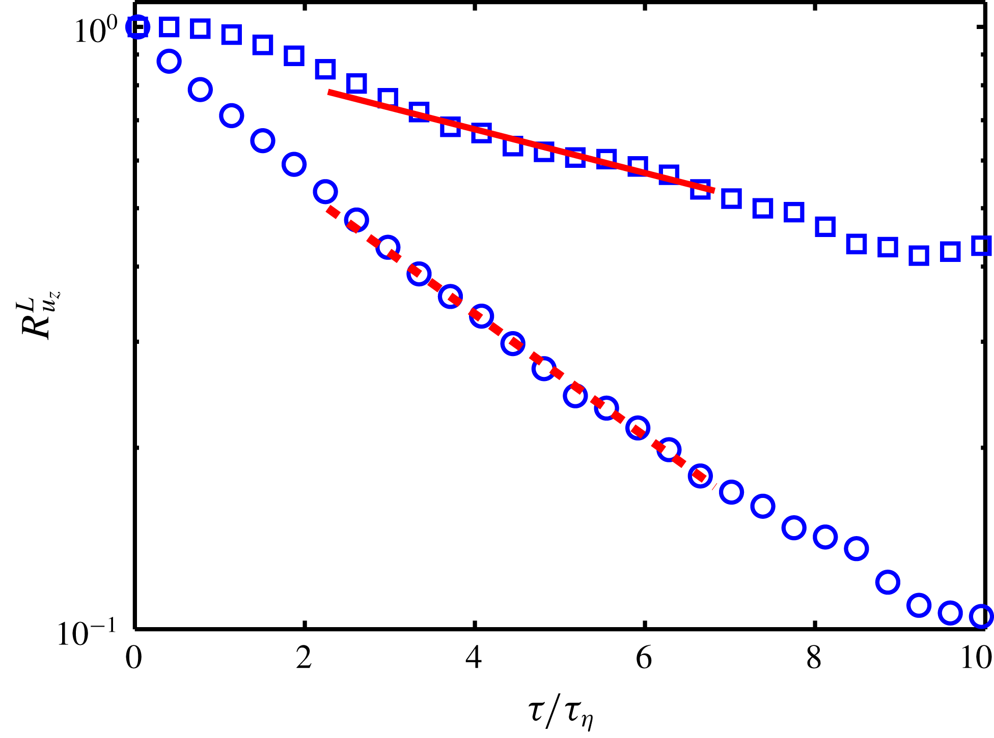
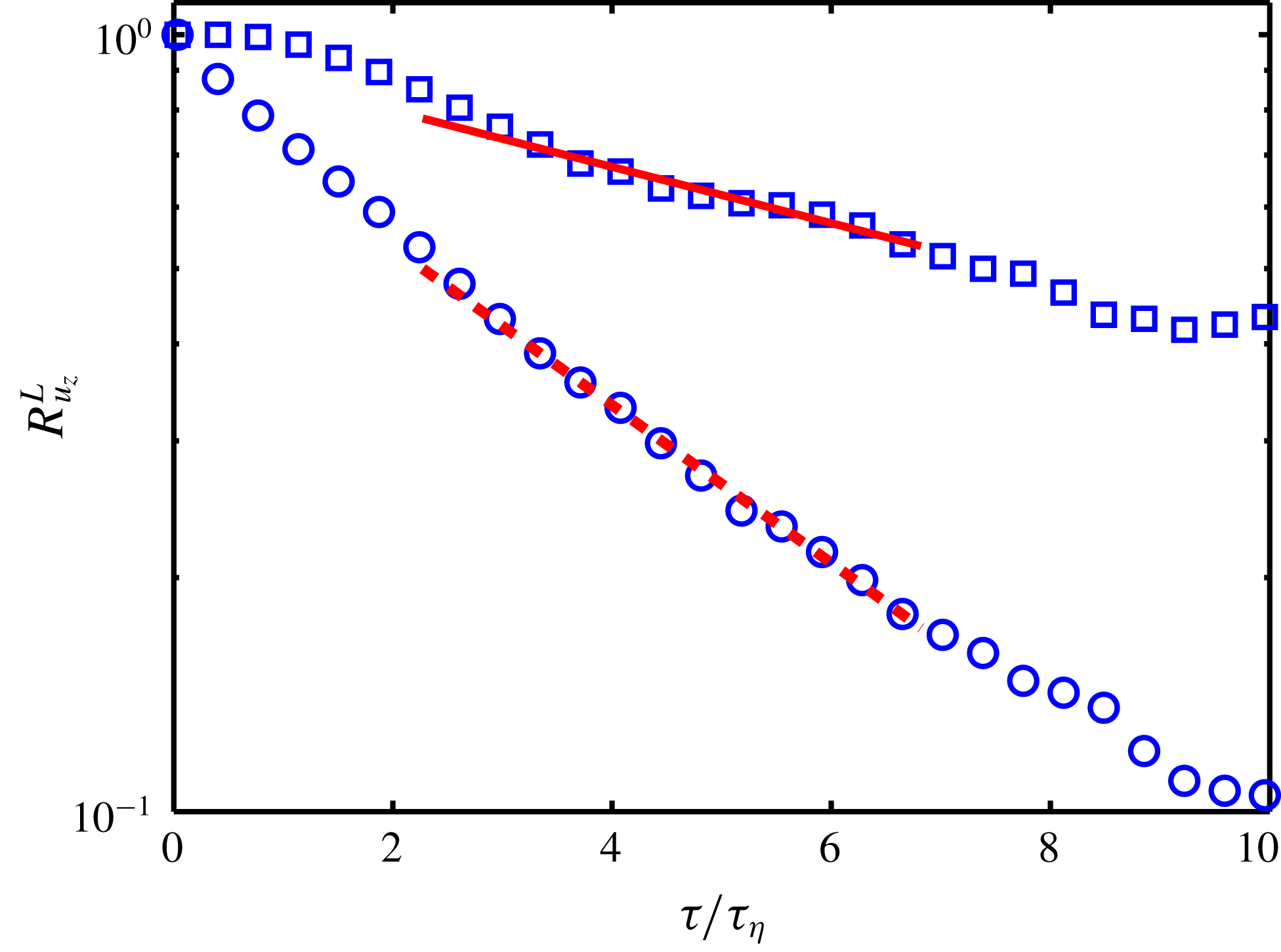
Detection of the plume and non-plume regions allows for differentiation between velocity autocorrelations inside and outside the plumes. Figure 6 shows the vertical velocity autocorrelations inside and outside the plumes for
 $Ro=0.048$
. In this figure, the open squares represent the vertical velocity autocorrelation of particles inside the plumes (
 $Q>0$
). The open circles, on the other hand, show the vertical velocity autocorrelation of the particles in non-plume regions (
 $Q\leqslant 0$
). The solid and dashed red lines are the fitted lines (proportional to
 $\text{e}^{-\unicode[STIX]{x1D70F}/\unicode[STIX]{x1D70F}_{0}}$
) through the open squares and circles, respectively. Clearly, the time scale for correlation within the plumes (the inverse slope of the solid red line) is larger than that for outside the plumes (the inverse slope of the dashed red line), indicating larger vertical flow coherence inside the plumes. The time scale values for different rotation rates computed with this method are given in figure 5 as open symbols.
It is worth mentioning that the solid symbols in figure 5 are calculated based on the velocity autocorrelation from the low particle concentration (LPC) data set while the plume detection method and consequently the open symbols are calculated based on the data from high particle concentration (HPC) experiments. Convergence for the large time lags of the HPC data set is questionable, thus the open symbols in figure 5 have inevitably larger uncertainties and the comparisons should be considered as qualitative; a one by one comparison might not be legitimate. However, the open and solid circles and squares clearly display similar trends.
It can be concluded that
 $\unicode[STIX]{x1D70F}_{1}$
in the vertical velocity autocorrelation (represented by the green line in the inset of figure 3
d), which is the governing time scale at small time lags
 $1\lesssim \unicode[STIX]{x1D70F}/\unicode[STIX]{x1D70F}_{\unicode[STIX]{x1D702}}\lesssim 6$
, is mainly determined by the flow time scale in the non-plume regions. Obviously, there is a contribution from the particles inside the plumes as well, however, this contribution is smaller since the number of particles in the non-plume regions is larger than that inside the plume. As has been shown, the particles in the non-plume regions decorrelate faster than those in the plume regions, e.g. the autocorrelation coefficient at
 $\unicode[STIX]{x1D70F}/\unicode[STIX]{x1D70F}_{\unicode[STIX]{x1D702}}=6$
is below 0.2 for the non-plume region compared to 0.5 for the plume region in figure 6. Thus, it is expected that the correlation at large time lags (
 $\unicode[STIX]{x1D70F}/\unicode[STIX]{x1D70F}_{\unicode[STIX]{x1D702}}\gtrsim 6$
) is mainly determined by the time scale
 $\unicode[STIX]{x1D70F}_{2}$
of the plume regions; the non-plume regions are already decorrelated for such large time lags. We interpret the time scale
 $\unicode[STIX]{x1D70F}_{2}$
of the plume regions as the residence time of the fluid parcel in a vortex, which is most probably closely related to the penetration time of fluid through columns.
Knowing that
 $\unicode[STIX]{x1D70F}_{1}$
is a characteristic correlation time of the flow outside the plumes, makes it possible to comment on the reason why
 $\unicode[STIX]{x1D70F}_{1}$
is constant while
 $\unicode[STIX]{x1D70F}_{2}$
increases with decreasing
 $Ro$
. As
 $\unicode[STIX]{x1D70F}_{1}$
is the correlation time outside the coherent structures, when
 $\unicode[STIX]{x1D70F}_{1}$
is non-dimensionalized by
 $\unicode[STIX]{x1D70F}_{\unicode[STIX]{x1D702}}$
, one would expect no significant changes with variation in turbulence intensity (i.e. variation in
 $Ro$
). On the other hand,
 $\unicode[STIX]{x1D70F}_{2}$
is the correlation time of the plumes which is found to vary with
 $Ro$
.
The vertical velocity autocorrelations for particles inside plumes (open squares) and outside plumes (open circles) for
 $Ro=0.048$
. The red solid and dashed lines are the exponential decays fitted through the open squares and circles, respectively. The fits are performed for
 $2\lesssim \unicode[STIX]{x1D70F}/\unicode[STIX]{x1D70F}_{\unicode[STIX]{x1D702}}\lesssim 7$
.
4.2 Concluding remarks
In conclusion, although the first transition (between regime I and II) is reflected in the velocity autocorrelations and the integral time scale (more profoundly near the top plate), the second transition (between regime II and III) is not as clearly reflected. This can be explained by the fact that the former transition is sudden while the latter transition appears to be more gradual. However, the cross-over to regime III coincides with the appearance of an additional correlation time scale in the vertical velocity autocorrelations near the top plate. Although the longer correlation time
 $\unicode[STIX]{x1D70F}_{2}$
increases with decreasing
 $Ro$
, the shorter time
 $\unicode[STIX]{x1D70F}_{1}$
remains constant. We have indicated that these two different correlation time scales are associated with the correlations inside and outside the plumes. The emergence of two correlation time scales suggest that the cross-over to regime III is caused by the presence of sufficiently strong plumes which interact less with their surroundings. In other words, the fluid exchange between plume and non-plume regions becomes considerably less in regime III. Thus, the plumes are separated from the non-plume regions; each characterized by their own time scale. The flow in regime III has therefore two distinct characteristics, one inside and another outside of the plumes. Further quantitative analysis of this hypothesis using detailed numerical simulations is encouraged.
5 Lagrangian r.m.s. acceleration
So far, the discussion has been on quantities which are largely determined by the large-scale flow field. In this section, however, we focus on the Lagrangian acceleration r.m.s. values which are governed by comparatively smaller scales.
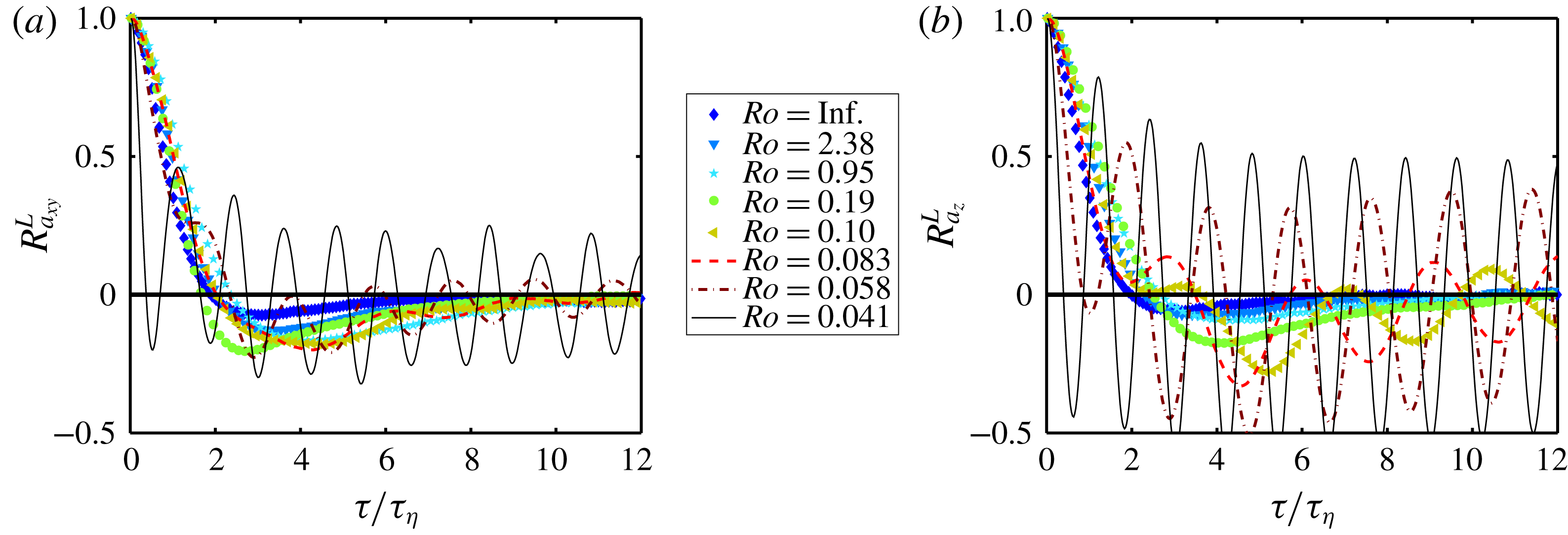
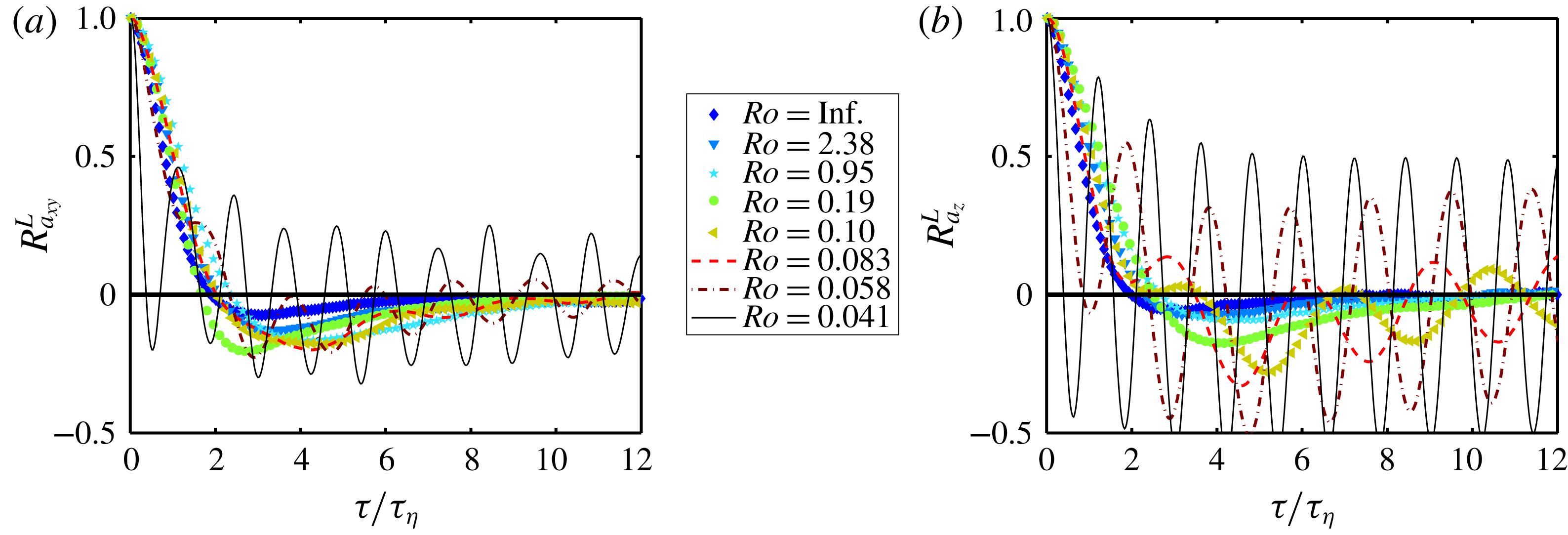
Prior to the analysis of the Lagrangian r.m.s. acceleration, we first focus on the undesired inertial waves emanating from precession forcing by the interplay of the applied rotation and Earth’s rotation. A discussion about the origin of these waves can be found in § 6. As mentioned before in § 4, a wavy behaviour in the horizontal velocity autocorrelation near the top plate is observed. Note that these waves are absent in the results of the numerical simulations (based on the Boussinesq approximation in a rotating frame of reference). The inertial waves have a minor effect on the velocity signal but as expected the effects of the waves are stronger on the acceleration signal. In order to illustrate these effects on the acceleration signal, we look into the Lagrangian acceleration autocorrelations. The Lagrangian acceleration autocorrelation is defined in a similar fashion as the Lagrangian velocity autocorrelation
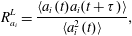 $$\begin{eqnarray}R_{a_{i}}^{L}=\frac{\langle a_{i}(t)a_{i}(t+\unicode[STIX]{x1D70F})\rangle }{\langle a_{i}^{2}(t)\rangle },\end{eqnarray}$$
where
 $a_{i}$
is the
 $i$
th component of the acceleration fluctuation of a fluid parcel. Figure 7 shows the Lagrangian acceleration autocorrelations for horizontal and vertical directions at the cell centre. The effect of the inertial waves are prominent in the Lagrangian acceleration autocorrelation. Therefore, it is expected that the acceleration fluctuations in regime III are also polluted by the presence of the inertial waves. In order to remove the approximate contribution of the inertial waves, we subtract the mean value of the acceleration of all particles in the measurement volume at each time step from the acceleration of each particle at that time step.
(a) Horizontal and (b) vertical acceleration autocorrelations at the cell centre as a function of
 $Ro$
.
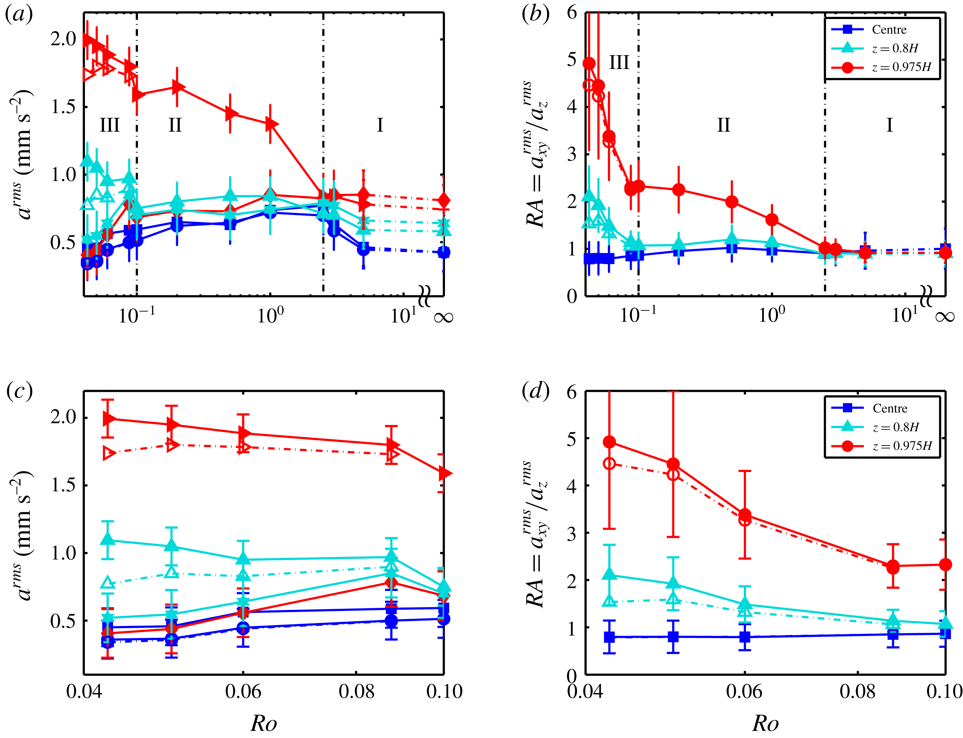
(a) Horizontal and vertical acceleration r.m.s. values from the experiments. Blue circles and squares are the horizontal and vertical components at the cell centre, respectively. Cyan upward-pointing triangles and stars are the horizontal and vertical components at
 $z=0.8H$
, respectively. Red right-pointing triangles and diamonds are the horizontal and vertical components at
 $z=0.975H$
. (b) The ratio
 $RA=a_{xy}^{rms}/a_{z}^{rms}$
as a function of
 $Ro$
. Experimental acceleration uncertainty (and thus the error bars) is estimated by adding noise to the displacement, see Rajaei et al. (Reference Rajaei, Joshi, Alards, Kunnen, Toschi and Clercx2016a
) for details. The open symbols in regime III are the acceleration fluctuations without the wave contribution. Panels (c) and (d) are extended views of regime III in (a) and (b), respectively.
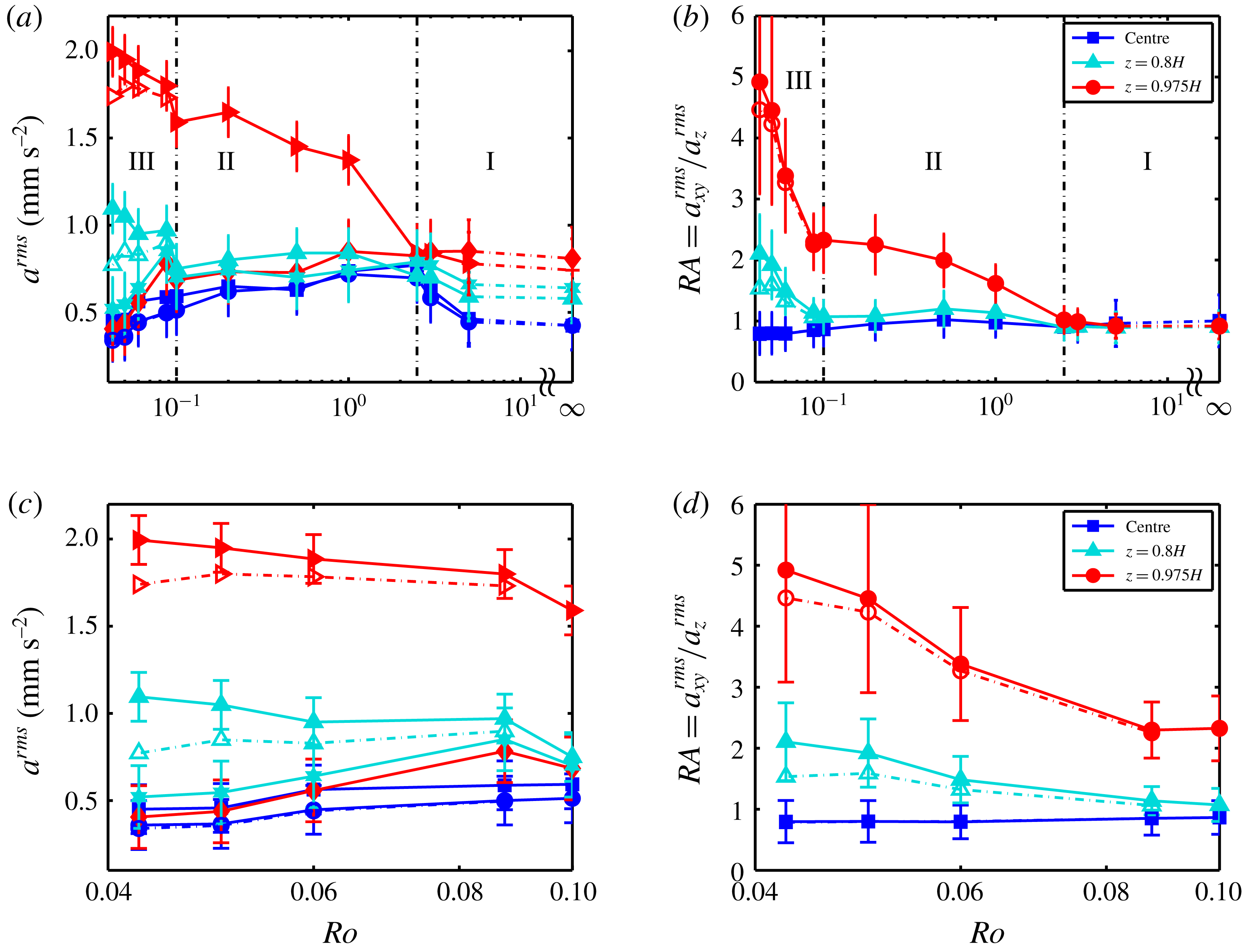
For the r.m.s. acceleration, similar to § 3, three different regions are analysed; the cell centre,
 $z=0.8H$
and
 $z=0.975H$
. The Lagrangian acceleration fluctuations and the ratio
 $RA=a_{xy}^{rms}/a_{z}^{rms}$
are plotted in figure 8(a,b). In regime III, the acceleration fluctuations without the wave contribution are also calculated; they are plotted as open symbols. For the data at the cell centre and several rotation rates at
 $z=0.8H$
and
 $z=0.975$
the open symbols are not visible because they almost collapse on the solid symbols. The acceleration fluctuation and its ratio in regimes I and II have been discussed in Rajaei et al. (Reference Rajaei, Joshi, Alards, Kunnen, Toschi and Clercx2016a
). Here, however, we focus on the acceleration fluctuation in regime III and the transition from regime II to III.
The horizontal and vertical components of the acceleration at the cell centre, see blue circles and squares in figure 8(a), continue to decrease as
 $Ro$
decreases due to the suppression of turbulence by the background rotation in regime III. The ratio
 $RA$
, which can also be used as a tool to partially evaluate small-scale isotropy, does hardly change while transitioning from regime II to regime III. The differences between open and solid symbols are negligible; they virtually collapse.
The measurements at
 $z=0.8H$
show that both horizontal and vertical accelerations decrease hardly in regime II with decreasing
 $Ro$
, resulting in an approximately constant
 $RA$
. However, after the transition to regime III, the horizontal component starts to increase in regime III due to the formation of strong vortical plumes capable of penetrating further into the bulk. The vertical component, on the other hand, keeps decreasing with decreasing
 $Ro$
in regime III, similar to regime II. As a result, the ratio
 $RA$
at
 $z=0.8H$
increases with decreasing
 $Ro$
in regime III: a clear indication that the vortical plumes are penetrating further into the interior region.
In regime III close to the top plate (
 $z=0.975H$
), the horizontal acceleration without the wave contribution shows a slight increase with decrease in
 $Ro$
, similar to that of regime II. The vertical acceleration, on the other hand, continues to decrease in regime III with decreasing
 $Ro$
, but at a higher decay rate compared to regime II. As a result, the ratio
 $RA$
increases in regime III at an even higher rate. The demarcation between regimes II and III is very well captured by the ratio
 $RA$
.
It is worth mentioning that the decrease in
 $a_{xy}^{rms}$
at the cell centre might not directly be related to whether vortical plumes reach the cell centre. Note that the sign of the vertical vorticity will flip as we move down far enough in a vortex column (Portegies et al.
Reference Portegies, Kunnen, van Heijst and Molenaar2008; Grooms et al.
Reference Grooms, Julien, Weiss and Knobloch2010); the vortical plumes spin down as they approach the centre which effectively reduces
 $a_{xy}^{rms}$
. The change in sign of vertical vorticity can be explained by the thermal-wind balance (Pedlosky Reference Pedlosky1979). Together with the decrease of the vertical vorticity, the plumes near the top and bottom walls are also squeezed due to the presence of the boundaries and widened due to conservation of angular momentum.
In conclusion, we can clearly see that the flow dynamics has changed while crossing to regime III near the top plate. If we assume that the vortical plumes interact considerably less in regime III (see the concluding remarks in § 4.2), a particle inside a plume stays inside the plume, thus experiencing a strong horizontal centripetal and weak vertical accelerations. In regime II, however, fluid parcels (particles) are exchanged between plume and non-plume regions more easily, resulting in a comparatively weaker horizontal centripetal acceleration. Therefore, the increase in the ratio
 $RA$
in regime III supports the conclusion drawn in § 4.2: there is less exchange between plume and non-plume regions in regime III.
Furthermore, the horizontal component of the r.m.s. acceleration at
 $z=0.8H$
starts to increase while crossing the transition point: the vortical plumes probably penetrate further into the bulk to form columns. However, at the cell centre the horizontal component of r.m.s. acceleration continues to decrease with decreasing
 $Ro$
in regime III.
6 Oscillatory behaviour
Wavy behaviours are observed in the Lagrangian velocity and acceleration autocorrelations. It is known that in a rotating frame, the Coriolis force promotes waves, so-called inertial waves (Greenspan Reference Greenspan1968). One can readily derive the dispersion relation from the inviscid linearized Navier–Stokes equations (Greenspan Reference Greenspan1968). Imposing boundary conditions makes the solutions dependent on the geometry; we focus on the cylindrical geometry. There are a variety of studies on inertial waves in a cylindrical geometry under different forcing mechanisms: steady differential rotation (Hart & Kittelman Reference Hart and Kittelman1996; Lopez & Marques Reference Lopez and Marques2010), forced sidewall oscillations (Lopez & Marques Reference Lopez and Marques2014), libration (Busse Reference Busse2010; Noir et al.
Reference Noir, Calkins, Lasbleis, Cantwell and Aurnou2010; Le Bars, Cébron & Le Gal Reference Le Bars, Cébron and Le Gal2015) and precession (Gans Reference Gans1970; Manasseh Reference Manasseh1992; Kobine Reference Kobine1995; Meunier et al.
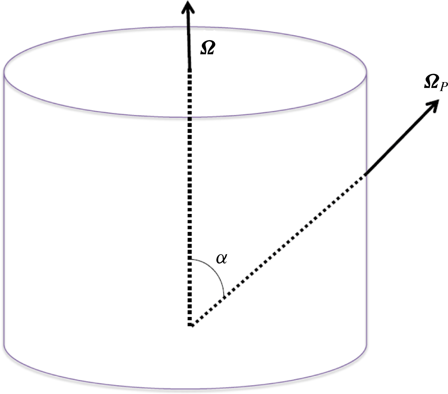
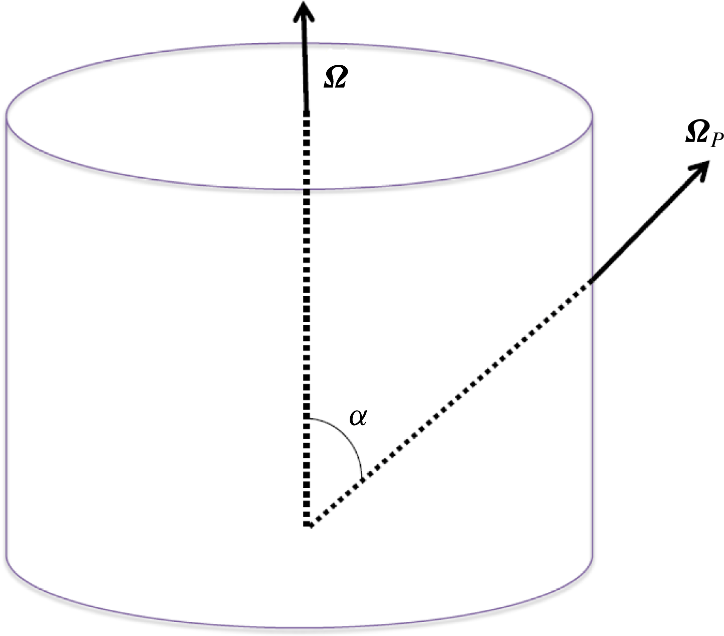
Reference Meunier, Eloy, Lagrange and Nadal2008; Liao & Zhang Reference Liao and Zhang2012). The first three conditions are not relevant for our experimental measurement. We consider the effects of precession due to Earth’s rotation in our experimental measurements. In precessing flows, a cylinder, filled with fluid, rotates about its axis while it precesses about another axis, see figure 9 for a schematic view of the problem. In this figure
 $\unicode[STIX]{x1D734}_{P}$
is the precession angular velocity,
 $\unicode[STIX]{x1D734}$
is the cylinder angular velocity and
 $\unicode[STIX]{x1D6FC}$
is the angle between
 $\unicode[STIX]{x1D734}$
and
 $\unicode[STIX]{x1D734}_{P}$
.
Sketch of the precessing flow.
 $\unicode[STIX]{x1D734}$
is the angular frequency of the cylinder and
 $\unicode[STIX]{x1D734}_{P}$
is the angular frequency of the precession.
The study of precessing flows is motivated by its relevance in the field of aerospace (propellant fuel in a spinning spacecraft e.g. Stewartson (Reference Stewartson1959), Agrawal (Reference Agrawal1993)) and atmospheric science (tornadoes and hurricanes (Vanyo Reference Vanyo2015)). In our experimental set-up, Earth’s rotation can act as the precession angular velocity. The important dimensionless parameters in precessing flows in cylindrical domains are the Ekman number, the Poincaré number and the aspect ratio (Liao & Zhang Reference Liao and Zhang2012). The Poincaré number is defined as
 $Po=|\unicode[STIX]{x1D734}_{P}|/|\unicode[STIX]{x1D734}|$
; in our case
 $|\unicode[STIX]{x1D734}_{P}|=|\unicode[STIX]{x1D734}_{Earth}|=7.292\times 10^{-5}~\text{rad}~\text{s}^{-1}$
and
 $\unicode[STIX]{x1D734}$
is the rotation rate of the rotating table,
 $\unicode[STIX]{x1D734}=\unicode[STIX]{x1D6FA}\hat{\boldsymbol{z}}$
, resulting in
 $1.8\times 10^{-5}\lesssim Po\lesssim 4.4\times 10^{-5}$
in regime III. The Poincaré number indicates the strength of precession (Wu & Roberts Reference Wu and Roberts2009) while the aspect ratio defines the resonance condition (Gans Reference Gans1970).
The momentum equation for precessing flow in cylindrical coordinates (
 $r,\unicode[STIX]{x1D719},z$
) is given in Liao & Zhang (Reference Liao and Zhang2012). One can readily write the momentum equation in dimensionless form. We can further simplify the dimensionless momentum equation when
 $Po\ll 1$
(weak precession),
 $Ro\ll 1$
and
 $\tilde{\boldsymbol{u}}<1$
(tilde stands for the dimensionless variable, the velocity is scaled with the free-fall velocity
 $U=\sqrt{\unicode[STIX]{x1D6FC}g\unicode[STIX]{x0394}TH}$
) (Liao & Zhang Reference Liao and Zhang2012)
 $$\begin{eqnarray}\frac{\unicode[STIX]{x2202}\tilde{\boldsymbol{u}}}{\unicode[STIX]{x2202}\tilde{t}}+\tilde{\boldsymbol{u}}\boldsymbol{\cdot }\tilde{\unicode[STIX]{x1D735}}\tilde{\boldsymbol{u}}+\frac{1}{Ro}\hat{\boldsymbol{z}}\times \tilde{\boldsymbol{u}}=-\tilde{\unicode[STIX]{x1D735}}\tilde{P}+\sqrt{\frac{Pr}{Ra}}\tilde{\unicode[STIX]{x1D6FB}}^{2}\tilde{\boldsymbol{u}}-\frac{Po}{4Ro^{2}}r\sin \unicode[STIX]{x1D6FC}\cos \left(\unicode[STIX]{x1D719}+\frac{\tilde{t}}{2Ro}\right)\hat{\boldsymbol{z}}+\tilde{T}\hat{\boldsymbol{z}}.\end{eqnarray}$$
As can be seen from the equation, the third term on the right-hand side, the so-called Poincaré forcing term, is the principal forcing term due to precession. To quantify the effects of Poincaré forcing on the flow field in our current experiments, direct numerical simulations with this precession forcing are performed at
 $Ra=1.3\times 10^{9}$
,
 $Pr=6.7$
,
 $Ro=0.058$
,
 $\sin \unicode[STIX]{x1D6FC}=0.6232$
(Eindhoven latitude
 $=$
51.44
 $^{\circ }$
) and corresponding
 $Po=\unicode[STIX]{x1D6FA}_{P}/\unicode[STIX]{x1D6FA}=2.51\times 10^{-5}$
. As in previous sections, tracer particles are tracked and evaluated.
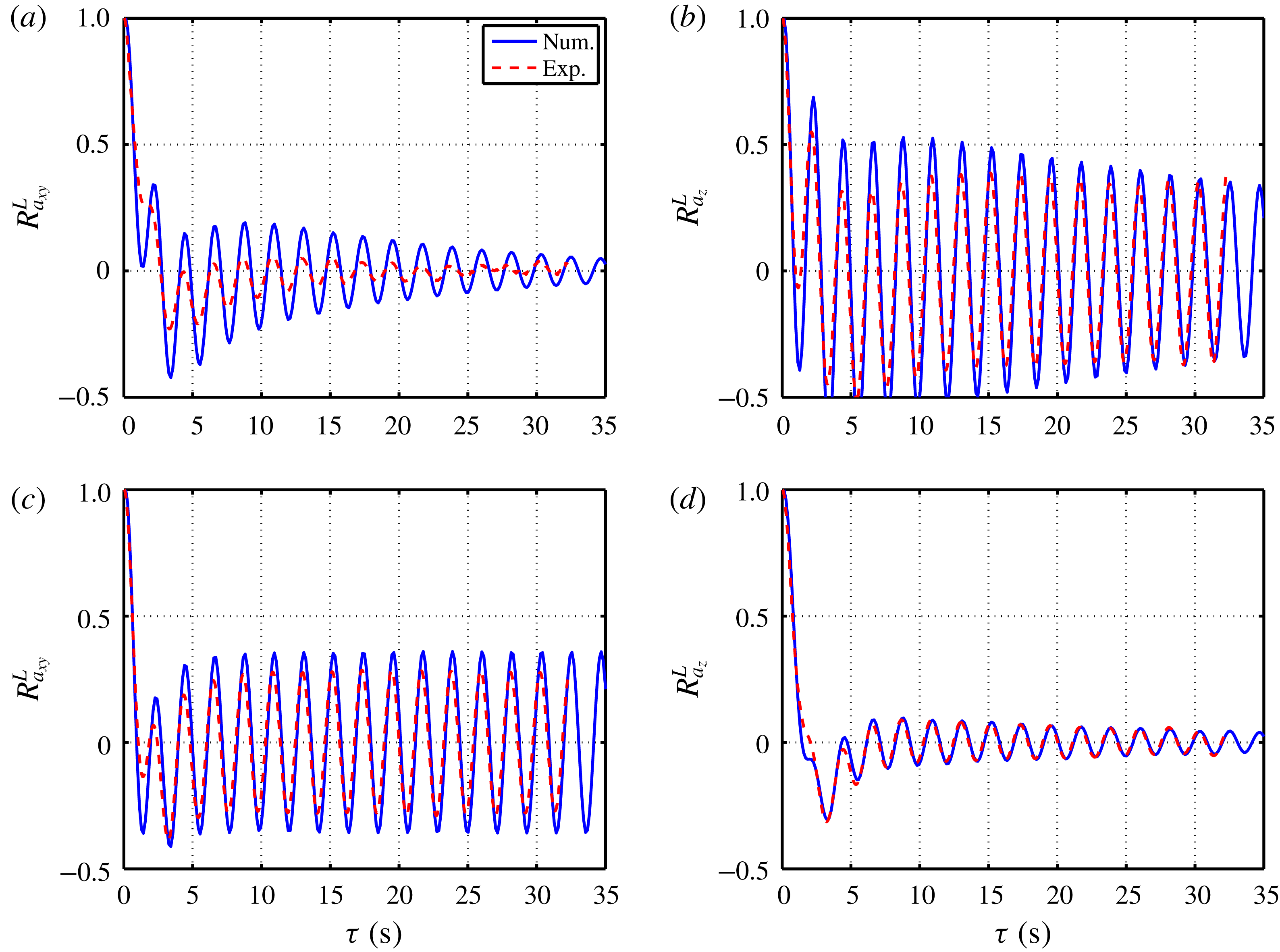
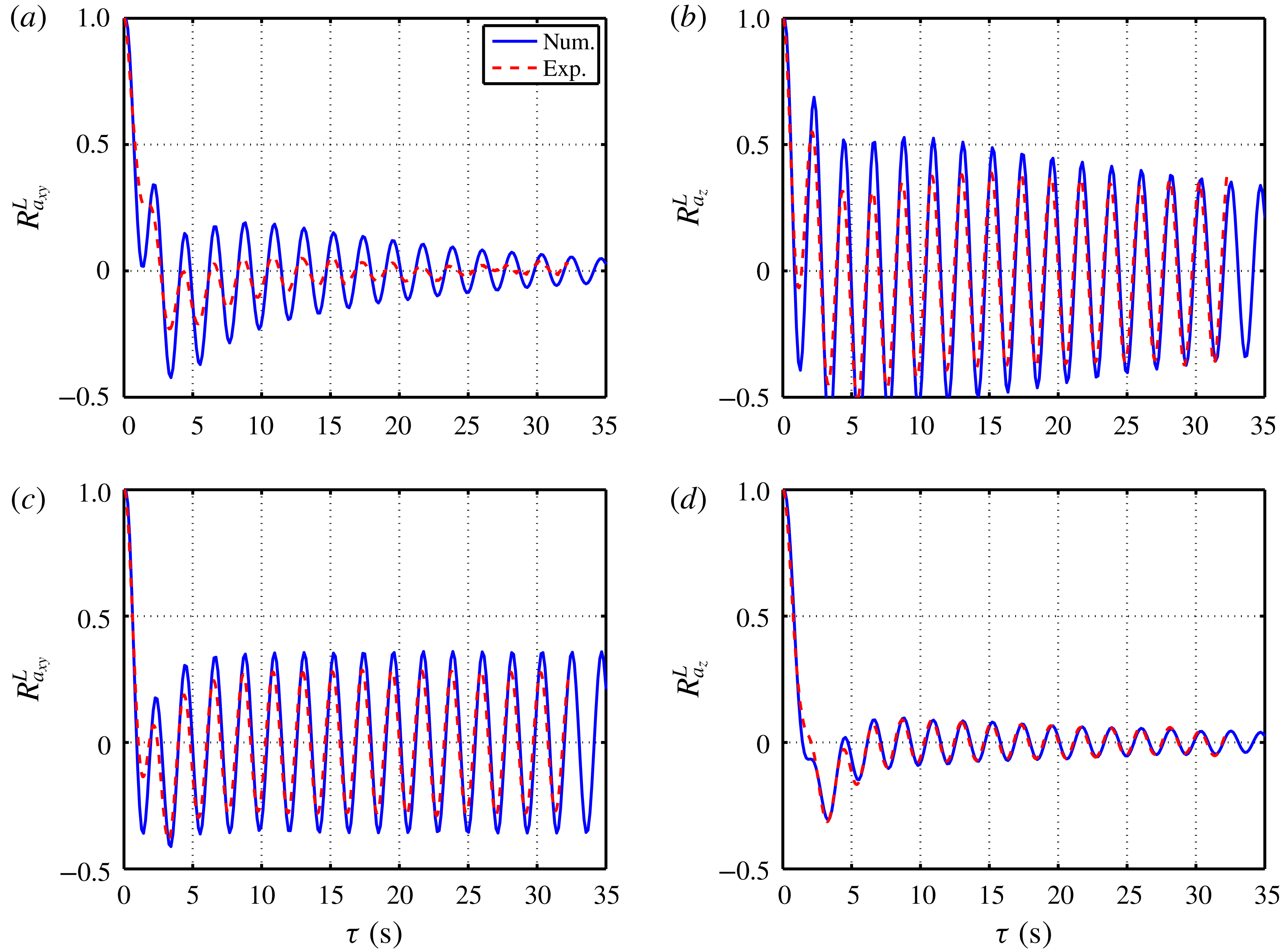
The experimental and corresponding numerical acceleration autocorrelations at the cell centre and at
 $z=0.875H$
are plotted in figure 10. The excellent agreement between experimental and simulation data confirms the role of the Poincaré force emanating from Earth’s rotation. The wave amplitudes are slightly different between experiment and numerical simulation, however, one should consider that the equations are simplified in the numerical simulations. The observed frequency in the acceleration autocorrelations is exactly
 $\unicode[STIX]{x1D6FA}$
in both the experiment and the numerical simulation. For an inviscid weakly precessing fluid, when the frequency of the primary inertial mode is the same as that of the Poincaré force (the frequency of Poincaré force is
 $\unicode[STIX]{x1D6FA}$
), a primary resonance happens. As shown by Meunier et al. (Reference Meunier, Eloy, Lagrange and Nadal2008) the primary resonance for a cylindrical cell with aspect ratio
 $\unicode[STIX]{x1D6E4}=1$
happens at a forcing frequency of
 $0.996\unicode[STIX]{x1D6FA}$
. Our forcing frequency is
 $\unicode[STIX]{x1D6FA}$
, very close to the primary resonance for
 $\unicode[STIX]{x1D6E4}=1$
. The primary resonances for
 $\unicode[STIX]{x1D6E4}=1/2$
and 2 are
 $0.49\unicode[STIX]{x1D6FA}$
and
 $1.57\unicode[STIX]{x1D6FA}$
, respectively. Note that these oscillations vanish when the Poincaré term in (6.1) is set to zero (Boussinesq approximation in rotating frame of reference).
Comparison of experimental and numerical acceleration autocorrelations. (a) Horizontal and (b) vertical acceleration autocorrelations at the cell centre. (c) Horizontal and (d) vertical acceleration autocorrelations at
 $z=0.875H$
.
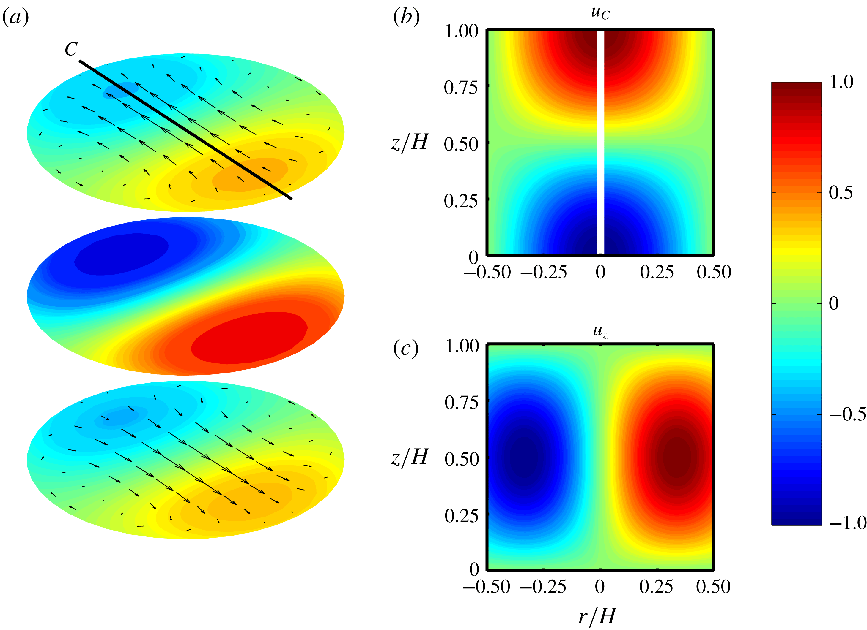
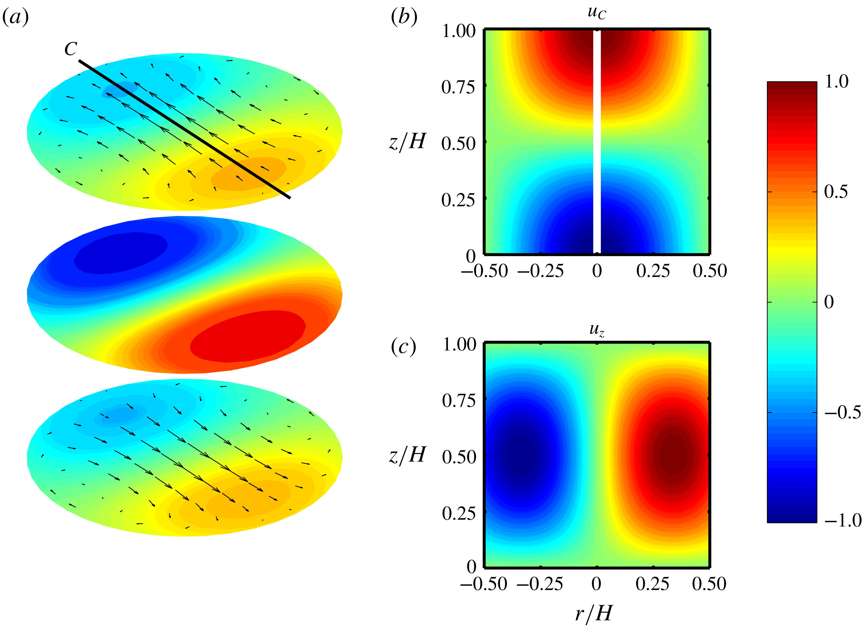
The velocity field belonging to the near-resonant inertial waves due to Poincaré forcing can be illustrated by plotting the solution of the wave equations. The wave equations and their solution are given in Meunier et al. (Reference Meunier, Eloy, Lagrange and Nadal2008). Figure 11(a–c) shows snapshots of the waves at time
 $t=0$
. Panel (a) shows the velocity of the waves at three cross-sections perpendicular to the rotation axis. The colours and arrows show the vertical and horizontal velocities, respectively. Two vertical cross-sections along line
 $C$
are presented in (b,c). The colours in panels (b) and (c) are the horizontal velocity along line
 $C$
and the vertical velocity, respectively. See the figure caption for more details. As can be seen from the graph, the horizontal component of the wave becomes stronger when approaching the top or bottom plates from the centre. The vertical component, on the other hand, is strongest at the cell centre and diminishes when departing from the centre. The same trend has been observed from experiments: strong vertical oscillations at the cell centre and strong horizontal oscillations near the top plate. This pattern rotates about the cylinder axis in an anticyclonic fashion at a rate
 $\unicode[STIX]{x1D6FA}$
. Note that these plots are formally for an inviscid flow; corrections for no-slip conditions in a realistic situation are restricted to minor boundary layer corrections (Meunier et al.
Reference Meunier, Eloy, Lagrange and Nadal2008).
Illustration of the dominant inertial wave mode in a
 $\unicode[STIX]{x1D6E4}=1$
cylinder. Panel (a) represents three cross-sections at
 $z=0.85H$
,
 $z=0.5H$
and
 $z=0.15H$
from top to bottom, respectively. The colours indicate the vertical velocity (perpendicular to the cross-sections) and arrows represent the horizontal velocity. The horizontal velocity at
 $z=0.5H$
is zero. (b) Shows a vertical cross-section along line
 $C$
, shown in (a). The colours indicate the horizontal velocity along line
 $C$
,
 $u_{C}$
. At
 $r/H=0$
the velocity
 $u_{C}$
is not defined. (c) Shows the vertical velocity in a vertical cross-section along line
 $C$
, similar to (b). The colour bar and consequently all the velocities are non-dimensionalized by their corresponding maximum velocities in each panel.
In conclusion, the observed oscillatory behaviour is emanating from precession by the Earth’s rotation: these waves are thus unavoidable. However, one can significantly reduce the amplitude of these waves by choosing a proper
 $\unicode[STIX]{x1D6E4}$
further from a resonant mode (Meunier et al.
Reference Meunier, Eloy, Lagrange and Nadal2008). Nonetheless, it was unfortunate that
 $\unicode[STIX]{x1D6E4}=1$
has a primary resonance at a driving frequency very close to
 $\unicode[STIX]{x1D6FA}$
. It is worth pointing out that the good agreement between experimental and numerical overall heat transfer measurements for small
 $Ro$
for
 $\unicode[STIX]{x1D6E4}=1$
, reported earlier in the literature (Stevens et al.
Reference Stevens, Zhong, Clercx, Ahlers and Lohse2009; Zhong et al.
Reference Zhong, Stevens, Clercx, Verzicco, Lohse and Ahlers2009), hint that the effects of these inertial waves on the heat transfer efficiency are negligible. However, one should note that the Poincaré forcing term increases with decreasing
 $Ro$
: the Poincaré force dominates over thermal forcing for small enough
 $Ro$
depending on
 $\unicode[STIX]{x1D6FC}$
. The Poincaré force is not limited to the thermally driven motions: it plays a role whenever the Poincaré force becomes comparable to the other means of forcing. Therefore, experiments in rapidly rotating flows should be done with special care: the geometry and its aspect ratio should be chosen accordingly.
7 Conclusions
In this paper, we have discussed different Lagrangian quantities in regimes I, II and III. In regime I, the presented results confirm the general picture of weakly rotating RBC flow: the flow dynamics is governed by the LSC. The changes in the velocity and acceleration statistics (r.m.s. and autocorrelations) both at the cell centre and near the top plate are relatively small in this regime.
According to the heat transfer efficiency, the transition from regime I to regime II is known to be sudden: The LSC is replaced by vortical plumes, in particular close to the wall and in the boundary layers. The r.m.s. velocity and acceleration and Lagrangian autocorrelations near the top plate experience a sudden change in trend while crossing this transition. On the other hand, the data at the centre show a gradual change between regime I and II; indicating that the transition starts near the plates, as has been shown earlier in Rajaei et al. (Reference Rajaei, Joshi, Alards, Kunnen, Toschi and Clercx2016a ).
The formation of the vortical plumes in regime II and columns in regime III is reflected in the Lagrangian velocity and acceleration statistics. The vertical velocity fluctuations decay faster than their horizontal counterparts at
 $z=0.8H$
and
 $z=0.975H$
. The integral time scales show an increase as
 $Ro$
decreases at the cell centre and near the top plate, except for the horizontal component near the top plate. The horizontal acceleration fluctuation near the top increases while the other components decrease with decreasing
 $Ro$
. All these observations are due to the formation of the vortical plumes and columns close to the top plate.
The transition between regimes II and III is comparatively gradual: the Lagrangian velocity statistics show gradual changes. However, the acceleration fluctuations show rather abrupt changes while crossing to regime III, keeping in mind that there is a contribution from inertial waves in the acceleration statistics. The cross-over to regime III coincides with the following phenomena and observations:
(i) The vertical motions are suppressed: The vertical component of the r.m.s. velocity and acceleration values are suppressed at a higher rate in regime III compared to regime II with decreasing
 $Ro$
. The suppression of the vertical motions result in a decrease in heat transfer efficiency.
(ii) The vortical plumes penetrate further into the bulk: the horizontal component of the r.m.s. acceleration continue to increases with decreasing
$Ro$
at
$z=0.975H$
, except for the lowest considered
$Ro$
. At
$z=0.8H$
, the horizontal component of the r.m.s. acceleration start to increase with decreasing
$Ro$
while transitioning to regime III: indicating that plumes have reached the interior region in regime III. At the cell centre, no enhancement in the horizontal component of the r.m.s. acceleration is observed. One should note that acceleration and velocity might not be perfect criteria for evaluating whether plumes reach the cell centre because it is known that as we go down inside a plume the sign of vorticity changes, e.g. a cold plume has a cyclonic vorticity near the top while it possesses an anticyclonic vorticity near the bottom plate. Therefore, the vorticity field is weaker in the cell centre resulting in a weaker swirling motion in the horizontal plane. This vertical change of vorticity can be explained with the thermal-wind balance. As a result, if the horizontal acceleration and velocity statistics at the centre do not follow their counterparts near the top, it does not directly imply that the plumes have not reached the cell centre.(iii) The vortical plumes interact less with their surroundings: two correlation time scales are present for plume and non-plume regions in regime III which indicates that the flow dynamics has distinct character inside and outside the plumes: the fluid exchange between plume and non-plume regions decreases in regime III for current
$Pr$
. In addition, a sudden increase in the ratio
$RA=a_{xy}^{rms}/a_{z}^{rms}$
at
$z=0.975H$
, observed in regime III, supports the same conclusion as the particles inside a plume remain inside the plume and experience a strong horizontal centripetal acceleration.


The first and second observations support the description of the transition to regime III by Julien et al. (Reference Julien, Knobloch, Rubio and Vasil2012a ). The last observation has not been reported earlier: it might be a key parameter to the transition. However, further experimental and numerical studies are certainly required to evaluate the different mechanisms.
Acknowledgements
This work is supported by the Nederland Wetenschappelijk Onderzoek (NWO), the Netherlands – formerly known as Stichting voor Fundamenteel Onderzoek der Materie (FOM). R.P.J.K. has received funding from the European Research Council (ERC) under the European Union’s Horizon 2020 research and innovation programme (grant agreement no. 678634). The authors would like to express special thanks of gratitude to A. Holten, G. Oerlemans, and F. van Uittert for assisting with the preparation of the experimental set-up.