1 Introduction
The structural organisation of turbulent wall-bounded flows has been a focus of researchers for several decades. Theodorsen (Reference Theodorsen1952) was probably the first to identify the presence of horseshoe shaped vortical structures originating at the wall at approximately
 $45^{\circ }$
. Kline et al. (Reference Kline, Reynolds, Schraub and Runstadler1967), after a series of quantitative and qualitative studies, observed the formation of low-speed streaks near the wall. They also showed that the streaks interact and this process, consisting of a lift up, an oscillation, a bursting and an ejection, suggests an instability mechanism that plays a key role in the transport of the turbulent kinetic energy. Following this work Corino & Brodkey (Reference Corino and Brodkey1969) used data from a pipe flow to analyse the structure near the wall, mainly highlighting the presence of fluid ejections in the region of
 $5<y^{+}<70$
, which interact with the mean flow (
 $y^{+}=yU_{\unicode[STIX]{x1D70F}}/\unicode[STIX]{x1D708}$
is the inner-normalised wall-normal position where
 $U_{\unicode[STIX]{x1D70F}}$
is the friction velocity and
 $\unicode[STIX]{x1D708}$
the viscosity of the fluid), and also a sweep event following right after (axial entry of fluid from upstream). Kim, Kline & Reynolds (Reference Kim, Kline and Reynolds1971) further established the occurrence of a series of events consisting of a low-speed streak lift, followed by an oscillation and a breakup, which they collectively called bursts. Wallace, Eckelmann & Brodkey (Reference Wallace, Eckelmann and Brodkey1972) using hot-film measurements in an oil-channel flow, introduced the quadrant classification of the streamwise–wall-normal plane,
 $u$
–
 $v$
(
 $u$
and
 $v$
denoting the streamwise and wall-normal velocity fluctuations respectively). They associated an upstream upwards motion (
 $u<0,v>0$
,
 $Q2$
event) with the ejection process identified earlier, and attributed the opposite combination (
 $u>0$
,
 $v<0$
,
 $Q4$
event) to a sweep type motion. However, it was not until 1975 that Offen & Kline (Reference Offen and Kline1975), while trying to establish a pattern for the bursting process, associated the lift up stage of the low-speed streak with the results of a vortex roll up and thus connected the depiction of the lifting process with the horseshoe vortex of Theodorsen (Reference Theodorsen1952). Strong experimental evidence for the presence of hairpin and horseshoe vortices was later provided by Head & Bandyopadhyay (Reference Head and Bandyopadhyay1981) who also observed that these structures were not clearly shaped for low Reynolds numbers where scale separation was small, but became increasingly elongated with higher Reynolds number. A comprehensive schematic of a hairpin vortex can be found in Adrian, Meinhart & Tomkins (Reference Adrian, Meinhart and Tomkins2000), where it is described as a structure with two counter-rotating legs (quasi-streamwise vortices) connected to the head of the vortex by vortex necks inclined at approximately
 $45^{\circ }$
with the wall.
Apart from analysing single structure behaviour, significant efforts were made to explain evidence of larger structures spreading in the logarithmic layer and the wake region (Brown & Thomas Reference Brown and Thomas1977), in the form of bulges with a mean streamwise extent reaching 2–
 $3\unicode[STIX]{x1D6FF}$
, where
 $\unicode[STIX]{x1D6FF}$
represents the boundary layer thickness (Kim & Adrian Reference Kim and Adrian1999). Even though the hairpin vortex model was able to incorporate several different observations throughout the years, some essential aspects – such as the large-scale motions mentioned above – could not be accounted for (Adrian et al.
Reference Adrian, Meinhart and Tomkins2000). This led researchers to look for clusters of structures, with Zhou et al. (Reference Zhou, Adrian, Balachandar and Kendall1999) recognising mechanisms of structure generation, followed with a forming of packets from single hairpin structures. The hairpin packet paradigm was thoroughly analysed by Adrian et al. (Reference Adrian, Meinhart and Tomkins2000), especially with respect to the packets’ growth and propagation. Several other studies further supported the existence of these large-scale motions (LSMs), reaching streamwise lengths of the order of 2–3
 $\unicode[STIX]{x1D6FF}$
(Christensen & Adrian Reference Christensen and Adrian2001; Ganapathisubramani, Longmire & Marusic Reference Ganapathisubramani, Longmire and Marusic2003; Wu & Christensen Reference Wu and Christensen2006; Adrian Reference Adrian2007, among others). Building on these observations, even larger, active motions in the outer layer were subsequently identified, reaching 8–16
 $R$
(Guala, Hommema & Adrian Reference Guala, Hommema and Adrian2006) and 12–14
 $R$
(Kim & Adrian Reference Kim and Adrian1999) in pipe flows, where
 $R$
is the pipe radius. In internal flows these motions are typically named very-large-scale motions (VLSMs), while in external flows the prevalent term is superstructures (Hutchins & Marusic Reference Hutchins and Marusic2007a
; Smits, McKeon & Marusic Reference Smits, McKeon and Marusic2011).
The passage of these clusters of structures described above was linked with an observed zonal structure of the flow in boundary layers. More specifically, Meinhart & Adrian (Reference Meinhart and Adrian1995) first described the organisation of a turbulent boundary layer into regions of uniform momentum which are bounded by internal layers of high shear. Adrian et al. (Reference Adrian, Meinhart and Tomkins2000) further argued that each zone is characterised by a ‘modal velocity’, which is the local peak of the probability density function (PDF) of the streamwise velocity component. They also suggested that these low momentum zones were the result of the passage of hairpin vortices and their packets, whose legs induce a backflow responsible for the lower momentum and whose heads lie on the high-shear regions that separate the zones. Kwon et al. (Reference Kwon, Philip, de Silva, Hutchins and Monty2014) used the modal peak-detection method proposed by Adrian et al. (Reference Adrian, Meinhart and Tomkins2000) to identify a region of uniform velocity magnitude in a channel flow. Later, Eisma et al. (Reference Eisma, Westerweel, Ooms and Elsinga2015), starting from the turbulent/non-turbulent interface (TNTI) in a boundary layer, reported the presence of internal layers below it, which they then linked to zones of uniform momentum. The term TNTI describes a region that separates a turbulent flow domain from an irrotational one. Such interfaces exist in many types of turbulent flows including jets, wakes and shear layers and also boundary layers. Starting from the work of Corrsin & Kistler (Reference Corrsin and Kistler1955) on free stream boundaries in turbulent shear flows, researchers have been increasingly interested in the properties of these interfaces (Phillips Reference Phillips1955; Turner Reference Turner1986; Westerweel et al. Reference Westerweel, Fukushima, Pedersen and Hunt2005; Hunt, Eames & Westerweel Reference Hunt, Eames and Westerweel2006; Westerweel et al. Reference Westerweel, Fukushima, Pedersen and Hunt2009; da Silva, dos Reis & Pereira Reference da Silva, dos Reis and Pereira2011; Ishihara, Ogasawara & Hunt Reference Ishihara, Ogasawara and Hunt2015, among others), their intermittent nature (Townsend Reference Townsend1949; Corrsin & Kistler Reference Corrsin and Kistler1955; Bisset, Hunt & Rogers Reference Bisset, Hunt and Rogers2002) and evolution (Kovasznay, Kibens & Blackwelder Reference Kovasznay, Kibens and Blackwelder1970; Khashehchi et al. Reference Khashehchi, Ooi, Soria and Marusic2013; Kwon et al. Reference Kwon, Philip, de Silva, Hutchins and Monty2014).
Based on the observations from these studies, Eisma et al. (Reference Eisma, Westerweel, Ooms and Elsinga2015) indicated that characteristics similar to those of TNTIs exist also in interfaces inside the boundary layer, which bound uniform momentum zones (UMZs), and whose growth rate is of the same order as that of the TNTI. Following the same conditional averaging techniques that have been commonly used to analyse the dynamics of the TNTIs, the authors found that these internal layers show a similar behaviour as the TNTIs, with the conditional averages of velocity, vorticity and Reynold’s stress exhibiting clear jumps, whose width grows with proximity to the wall. They further showed that the layers move upwards faster with increasing distance from the wall, based on theoretical concepts for the computation of the entrainment velocities. Later, de Silva, Hutchins & Marusic (Reference de Silva, Hutchins and Marusic2016) analysed the presence of UMZs within these internal layers, and showed that their number increases logarithmically with Reynolds number, their thickness diminishes closer to the wall, and their organisation can be approximately described by the attached eddy model (Perry & Chong Reference Perry and Chong1982).
In the present work, the focus is mainly on the temporal characteristics of UMZs, assessed using time-resolved planar particle image velocimetry (PIV) measurements of a turbulent boundary layer. After a brief description of the experimental details, a short outline on the instantaneous detection of modal peaks is presented, following the work of both Adrian et al. (Reference Adrian, Meinhart and Tomkins2000) and de Silva et al. (Reference de Silva, Hutchins and Marusic2016). The detection process is then extended to account for temporal coherence of UMZs. Results on the velocity range and thickness of the time-coherent UMZs, according to their relative position within the boundary layer and the total number of zones within a snapshot, are presented. Residence times of individual zones, within the measurement plane, are subsequently analysed and their dependence on modal velocity and the total number of zones within a snapshot are also discussed. Finally, a conceptual model is developed that summarises the structural characteristics of the two different flow states observed in the extreme cases of high and low number of zones.
2 Experimental set-up
Time-resolved planar PIV experiments in a turbulent boundary layer were carried out in the recirculating water channel (
 $1.2\times 0.8\times 6.75~\text{m}$
) located at the University of Southampton. The centre of the measurement plane was 5.5 m downstream of the contraction’s end where the flow was tripped with 10 cm wide 60-grit sandpaper. For the seeding,
 $56~\unicode[STIX]{x03BC}\text{m}$
polyamide particles (Vestosint 2157) were used, resulting in particle images of
 $2$
pixels. A plane, approximately
 $0.07\times 0.22~\text{m}$
, in the streamwise and wall-normal direction respectively (denoted hereafter
 $x$
and
 $y$
), was illuminated with a Litron LDY
 $304$
laser and images were acquired with a Phantom v641 32 GB camera, with a
 $2560\times 1600$
pixel sensor, fitted with a Sigma f/2.8 EX DG Macro lens with a focal length of 105 mm resulting in a digital resolution of
 $11~\text{pixels}~\text{mm}^{-1}$
. The average pixel displacement in the streamwise direction in the free stream was approximately
 $14$
pixels. A LaVision High Speed Controller was used to synchronise the system. We acquired 405 000 images (in 37 independent time-resolved sets of 10 947 images, covering approximately 500 s of flow in total) at 800 Hz, which we subsequently processed with the same software using iterative correlation with a final interrogation window of
 $16\times 16~\text{pixels}$
(
 $1.4\times 1.4~\text{mm}$
) and an overlap factor of 50 %. DaVis 8.2 was used for acquisition and processing. Approximately 96 % of the final vectors were a first choice, while the total percentage of interpolated vectors was below 1 %.
The nominal flow conditions, assessed over all images, were:
 $U_{\infty }=0.99~\text{m}~\text{s}^{-1}$
,
 $\unicode[STIX]{x1D6FF}=0.14~\text{m}$
(
 $\unicode[STIX]{x1D6FF}_{99}=0.12~\text{m}$
),
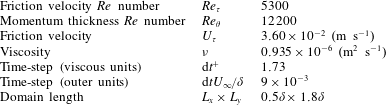
 $Re_{\unicode[STIX]{x1D70F}}=5300$
, while the resulting field of view (FOV) was approximately
 $0.5\unicode[STIX]{x1D6FF}\times 1.8\unicode[STIX]{x1D6FF}$
in the streamwise and wall-normal direction respectively (Table 1). The friction velocity was computed using the Clauser chart method (Clauser Reference Clauser1954), while the boundary-layer height was estimated based on Jones’ integral (Jones, Marusic & Perry Reference Jones, Marusic and Perry2001). The uncertainties involved in the computation of the mean quantities and Reynolds shear stress, following Sciacchitano & Wieneke (Reference Sciacchitano and Wieneke2016), were
 $\unicode[STIX]{x1D716}_{U}=0.8\,\%$
,
 $\unicode[STIX]{x1D716}_{V}=0.2\,\%$
and
 $\unicode[STIX]{x1D716}_{u^{\prime }v^{\prime }}=0.02\,\%$
, for the mean streamwise and wall-normal velocity components and the Reynolds shear stress respectively (percentages with respect to the free stream velocity,
 $U_{\infty }$
). Due to the high acquisition frequency, the dataset was additionally filtered in time, using a moving-average filter with a window length of 3 points in time resulting in an effective time step of
 $\text{d}t^{+}=5.1$
, following the temporal resolution limits discussed by Hutchins et al. (Reference Hutchins, Nickels, Marusic and Chong2009). Pixel-locking effects have been shown to influence the identification of UMZs, which is crucial to our analysis (see Kwon et al.
Reference Kwon, Philip, de Silva, Hutchins and Monty2014; de Silva, Marusic & Hutchins Reference de Silva, Marusic and Hutchins2014; de Silva et al.
Reference de Silva, Hutchins and Marusic2016). Thus, the temporal filtering applied to the data, also served to mitigate the bias error due to the pixel locking inherent in the PIV images. Further to that, and based on the initial vector overlap (50 %), a spatial two-dimensional Gaussian filter with a
 $3\times 3$
point kernel was also applied (with a standard deviation
 $\unicode[STIX]{x1D70E}_{G}^{+}=50$
), such that the effective spatial resolution of the data remained largely unaltered. After both spatial and temporal filtering, the resulting velocity PDF showed that the pixel-locking effects were mostly suppressed (see also de Silva et al.
Reference de Silva, Marusic and Hutchins2014).
Nominal flow conditions and domain size.

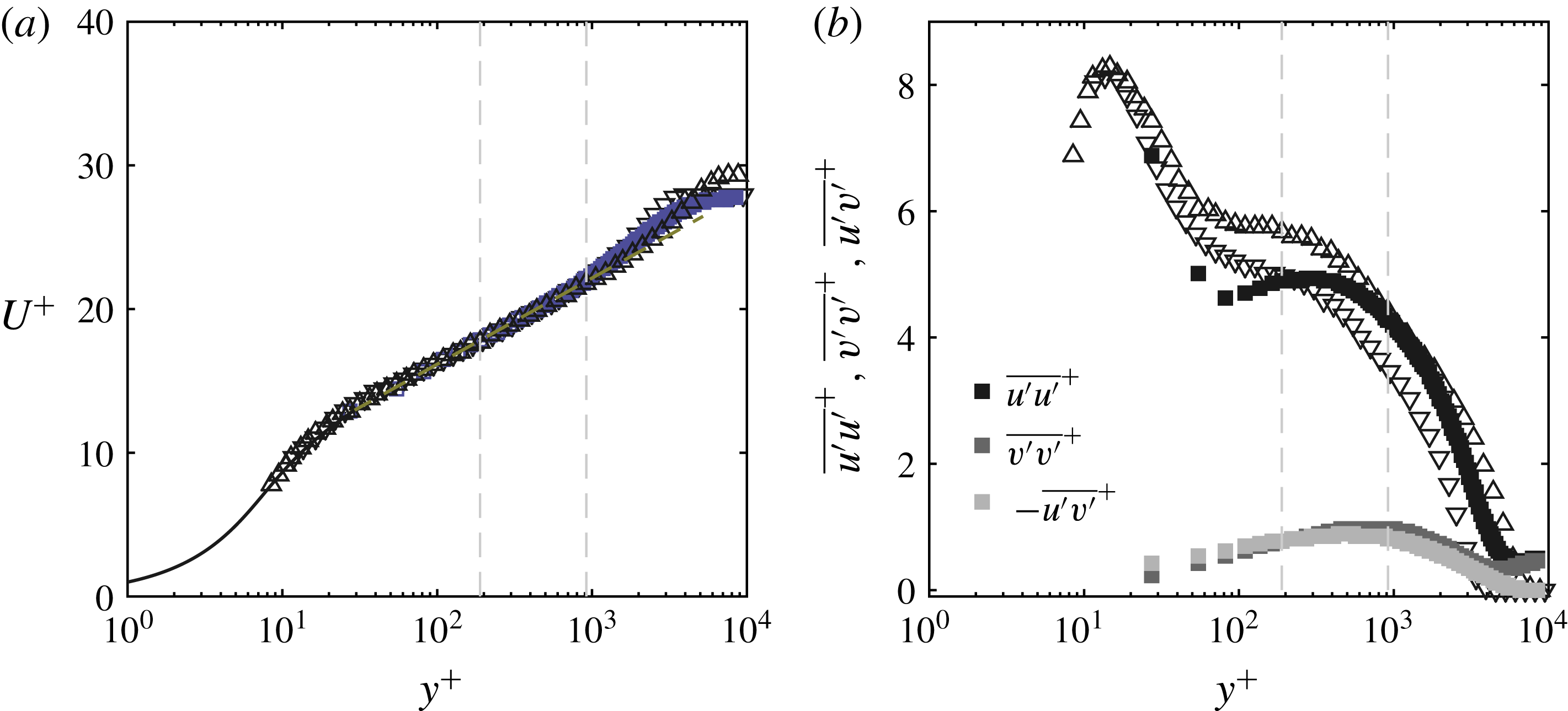
(a) Inner-normalised mean velocity profile. Solid black line indicates Spalding’s law of the wall for the near-wall region. (b) Inner-normalised turbulence intensity profiles of the streamwise and wall-normal components and Reynolds shear stress profile. Triangles are hot-wire data from Hutchins et al. (Reference Hutchins, Nickels, Marusic and Chong2009).

The mean velocity profile displayed a log region (
 $\unicode[STIX]{x1D705}=0.38$
,
 $B=4.1$
) for
 $200<y^{+}<0.18\unicode[STIX]{x1D6FF}$
(figure 1
a). For the computation of the momentum thickness,
 $\unicode[STIX]{x1D703}$
, Spalding’s law of the wall (Spalding Reference Spalding1961) was employed for the region from the wall up to the first independent velocity point (i.e. the first point not influenced by the wall in the image correlation process). Turbulence intensity profiles of the streamwise and wall-normal components, as well as the Reynolds shear stress profile, are shown in figure 1(b), together with streamwise turbulence intensity profiles from hot-wire data (Hutchins et al.
Reference Hutchins, Nickels, Marusic and Chong2009) of a turbulent boundary layer with a higher and lower Reynolds number (
 $Re_{\unicode[STIX]{x1D70F}}=3910$
and 7340). The profile of the current dataset lies in between those of the two hot-wire datasets for the largest part of the boundary layer. Spatial resolutions effects, inherent to PIV, can be seen close to the wall, however since large structures (UMZs) are of interest here, these effects are not expected to influence the presented results. The free stream turbulence intensity was approximately
 $3\,\%$
(typically elevated in water channels compared to wind tunnels).
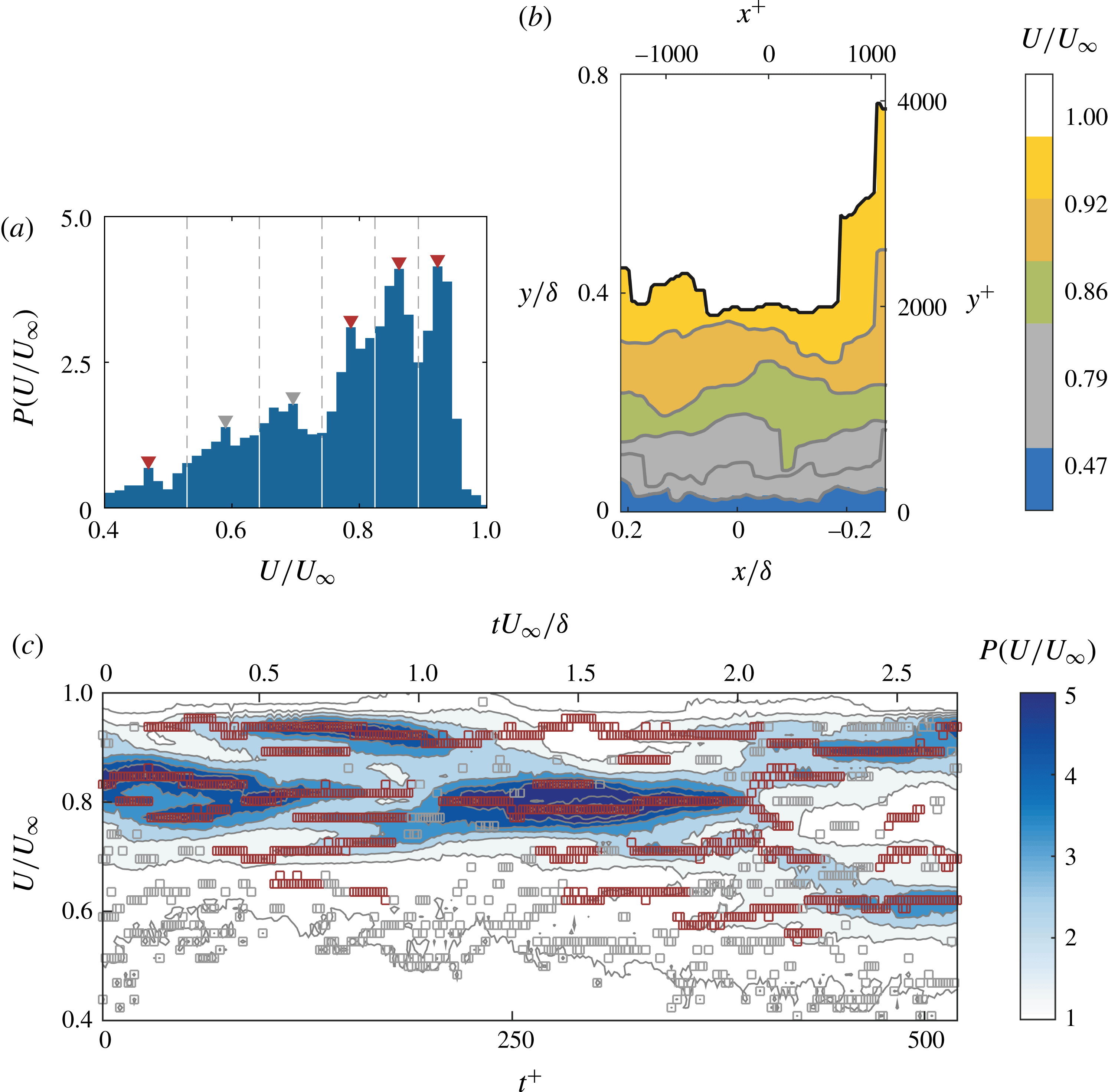
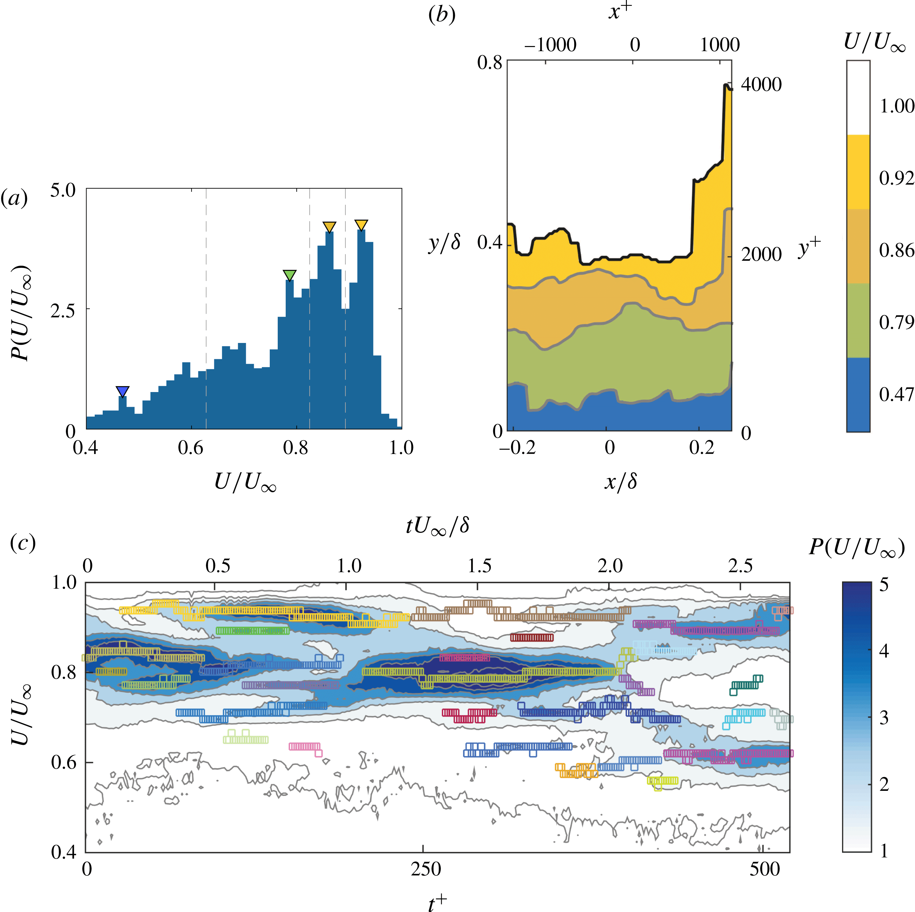
(a) The PDF of
 $U/U_{\infty }$
for an instantaneous velocity field. Triangles denote all detected modal velocities for this field, each corresponding to an instantaneous UMZ; dark red for time-coherent peaks and grey for short-lived ones. Grey dashed lines denote the velocity values that demark each zone. (b) Corresponding contour plot of each detected UMZ. Colours represent modal velocities of time-coherent zones; short-lived zones are denoted with grey. The TNTI is marked with solid black line and the boundaries of each UMZ with solid grey line. (c) Contour plot of the time evolution of the PDF of
 $U/U_{\infty }$
, for 300 consecutive images. Contour lines ranging from 0.3 to 7.5 with a spacing of 0.8. Grey and red squares represent short-lived and time-coherent peaks respectively.

3 Detection methods
3.1 Instantaneous zones
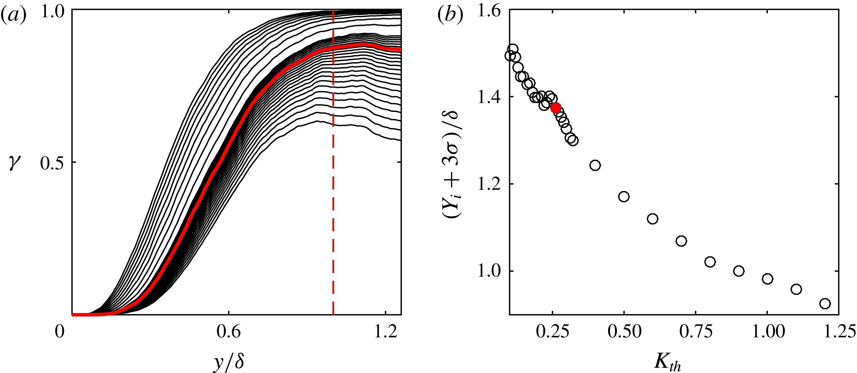
In order to identify the instantaneous UMZs and the layers that separate them, we follow the methodology used by Adrian et al. (Reference Adrian, Meinhart and Tomkins2000) and de Silva et al. (Reference de Silva, Hutchins and Marusic2016), extended to exploit the time-resolved information captured in the present experiment. The instantaneous method is based on detecting the local peaks of the PDF of the streamwise velocity component for every velocity snapshot. However, as suggested by de Silva et al. (Reference de Silva, Hutchins and Marusic2016), only the vectors below the turbulent/non-turbulent interface (TNTI) are included, so that the significantly higher outer peak of the non-turbulent region would not overshadow the ones of the UMZs. For the detection of the TNTI, we choose to use a kinetic energy deficit threshold, as described in Chauhan, Philip & Marusic (Reference Chauhan, Philip and Marusic2014a ), Chauhan et al. (Reference Chauhan, Philip, de Silva, Hutchins and Marusic2014b ) (for more details see appendix A). After the TNTI location is estimated, the vectors belonging to the turbulent region can be identified for every velocity snapshot, and the PDF of the streamwise velocity component can be constructed (see figure 2 a). It has been shown that points of local maxima represent the modal velocities that characterise each UMZ (Adrian et al. Reference Adrian, Meinhart and Tomkins2000; de Silva et al. Reference de Silva, Hutchins and Marusic2016). In order to define the edges of the UMZs in physical space, velocity contours at points of local minima in the PDF can be used. Because the zones and their edges are treated independently, it is not always certain that each peak would be bounded by two edges, so for the peaks that are unbounded, the mid-distance between two peaks is chosen as the edge location (see de Silva et al. Reference de Silva, Hutchins and Marusic2016). A representative example of this procedure can be seen in figure 2. Local peaks in the velocity PDF (triangles in figure 2 a) correspond to each zone’s modal velocity. The velocities at the points between neighbouring peaks (grey dashed lines in figure 2 a) are used to define the contour lines demarcating each UMZ in physical space (solid grey lines in figure 2 b). Repeating this process for consecutive snapshots, the temporal coherence of each detected peak can be analysed (figure 2 c). From a temporal perspective it can be seen that some modal peaks reside within our FOV for very short times (grey symbols in figures 2(a), 2(c) and grey coloured layers in figure 2 b), while others reside for much longer (red symbols in figures 2 a, 2 c and coloured layers in figure 2 b). A detailed discussion on this distinction follows in the next section.
There are some important considerations regarding the instantaneous detection process and the resulting number of peaks (
 $N_{UMZ}$
), that are worth discussing briefly here. Firstly, the streamwise extent of the data and consequently the number of vectors available, were shown by de Silva et al. (Reference de Silva, Hutchins and Marusic2016) to be important factors when detecting the modal velocities. In our case, the available streamwise extent is
 ${\approx}$
2600 viscous units (
 $0.5\unicode[STIX]{x1D6FF}$
), including on average 6500 vectors below the TNTI (depending on its vertical location). For the construction of the PDF, the vectors are distributed in 67 bins with size approximately equal to
 $0.5U_{\unicode[STIX]{x1D70F}}$
, for
 $U/U_{\infty }\in [0,1]$
. However, it should be noted that, due to spatial resolution effects, only the last 50 bins with
 $U/U_{\infty }\in [0.26,1]$
are relevant here; no peaks in the PDF are detected for lower velocities. We choose to use the full streamwise extent available for the detection process. However for completeness, we also repeated the process with a reduced streamwise extent of 2000 viscous units; even though there were instantaneous discrepancies in individual snapshots, the resulting statistics were very similar while the trends discussed in the following sections remained unaltered.
Aside from the streamwise extent and number of vectors used, the thresholds used in the peak-detection algorithm itself, are the most important factors in the resulting number of peaks. These include the allowed distance between two peaks
 $F_{d}$
, (in integer multiples of the bin width), the minimum height for a peak to be considered detectable,
 $F_{h}$
, and the difference in height of a given peak relative to its neighbouring points (prominence),
 $F_{p}$
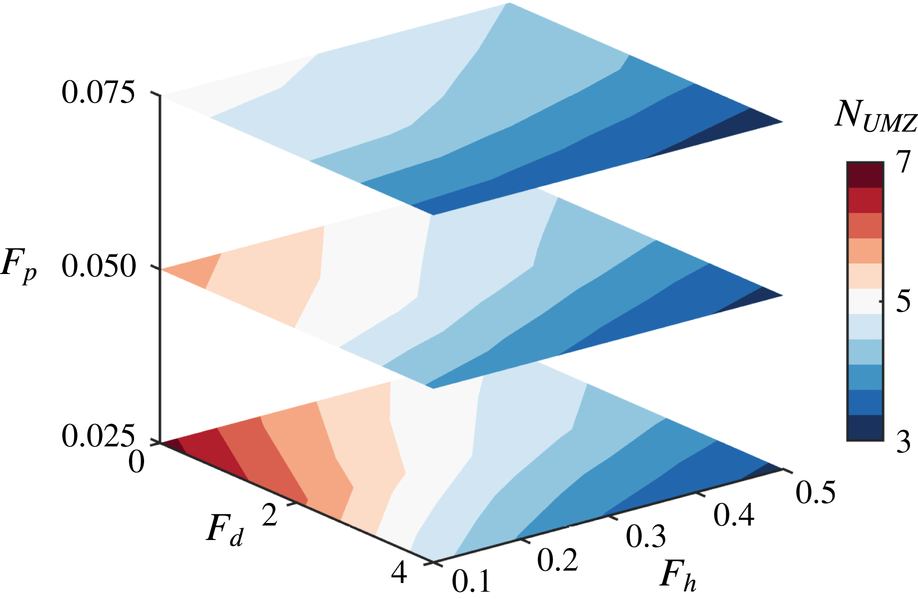
. Depending on these parameters, the resulting average number of detected peaks is found to vary significantly (figure 3). An increase of the minimum required prominence of the peaks with respect to their neighbours results in a gradual decrease of the average detected number of peaks (from 6 to almost 3), as expected. Similarly, when the allowed distance between peaks is significantly increased, no more than 4 peaks on average can be detected. When the peaks are allowed to be next to each other, however, the number of detected peaks can reach up to 7, although in that case differentiating between different UMZs would be almost impossible. Finally, the range of the minimum required peak heights tested here, seemed to have an imperceptible influence on the resulting number of peaks (increasing height leads to slightly lower
 $N_{UMZ}$
). It should be noted that the trends discussed in the following sections are robust to the chosen values for these thresholds and are meant to show relative changes rather than represent an absolute value of
 $N_{UMZ}$
(see also de Silva et al.
Reference de Silva, Hutchins and Marusic2016).
Contours of the average number of peaks detected, with varying minimum peak height,
 $F_{h}$
, minimum peak distance,
 $F_{d}$
, and minimum peak prominence from neighbouring points,
 $F_{p}$
, in the peak-detection algorithm.

In order to facilitate comparison with previous results, we choose a parameter set such that the average number of peaks follows the Reynolds number dependency found by de Silva et al. (Reference de Silva, Hutchins and Marusic2016). These include a minimum peak height of 0.3 with a prominence of at least 0.05 from neighbouring values, and a minimum distance of two bins between detected peaks. We apply this detection process to all the available velocity snapshots independently and, on average
 ${\approx}4.5$
peaks are detected for
 $Re_{\unicode[STIX]{x1D70F}}=5300$
, with a distribution that follows the results of de Silva et al. (Reference de Silva, Hutchins and Marusic2016).
3.2 Time-coherent zones
Following the process described above, we can successfully identify UMZs and their edges in all available snapshots, however tracking them in time becomes increasingly difficult for several reasons. From a physical perspective, even when identified correctly, not all modal velocities and zones that appear instantaneously necessarily last longer than a single snapshot in time. Furthermore, while identifying local maxima in independent distributions can be successful most of the time, following the same procedure in a time series does not always result in a smooth evolution of the detected peaks. For these reasons, to identify the peaks and edges in the time-resolved data available, we still use an instantaneous detection for each velocity snapshot, but we further set a temporal threshold (
 $\unicode[STIX]{x1D70F}^{+}\approx 20$
) to remove peaks that remain within the measurement plane for short times (referred to as residence times,
 $\unicode[STIX]{x1D70F}$
). Since the characteristic velocity (modal velocity) of each peak is the basis of its instantaneous detection, we also use it to evaluate its temporal coherence. More specifically, peaks that are detected in successive snapshots and vary their modal velocity within a band of
 $\pm 0.5U_{\unicode[STIX]{x1D70F}}$
(corresponding to a shift of a single bin in the velocity PDF in either direction) from one snapshot to the other, are considered coherent between these snapshots. The effect of this procedure can be seen by contrasting figures 2 and 4; short-lived peaks have been removed in the latter. A video representing the evolution of both short-lived and time-coherent peaks can be found in the supplementary material (movie 1) available at https://doi.org/10.1017/jfm.2018.126. Short-lived peaks are denoted with grey colours while the time-coherent peaks are coloured according to their modal velocity.
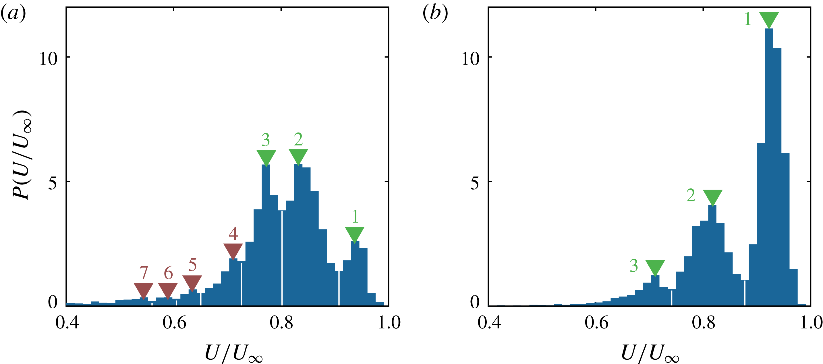
(a) The PDF of
 $U/U_{\infty }$
, (b) corresponding contour plot of each detected zone and (c) time evolution of the PDF of
 $U/U_{\infty }$
for the same velocity frames as in figure 2, when all short-lived peaks are removed. Coloured symbols and contours in (a) and (b) respectively, represent the modal velocity of each UMZ. The individual temporal evolution of each UMZ is separately coloured in (c) with contour lines ranging from 0.3 to 7.5 with a spacing of 0.8.

The chosen temporal threshold, taking into account the initial temporal filter applied (resulting in an effective time step of
 $\text{d}t^{+}=5.1$
), ensures that a UMZ is present in at least 4 consecutive snapshots. It is important to note that, a spatial filter has already been used for the detection of the UMZs, in the form of the instantaneous PDFs, which include all the vectors of each snapshot spanning
 $0.5\unicode[STIX]{x1D6FF}$
in the streamwise direction. Therefore, results presented here refer to structures spanning at least
 $0.5\unicode[STIX]{x1D6FF}$
in length (
 ${\approx}$
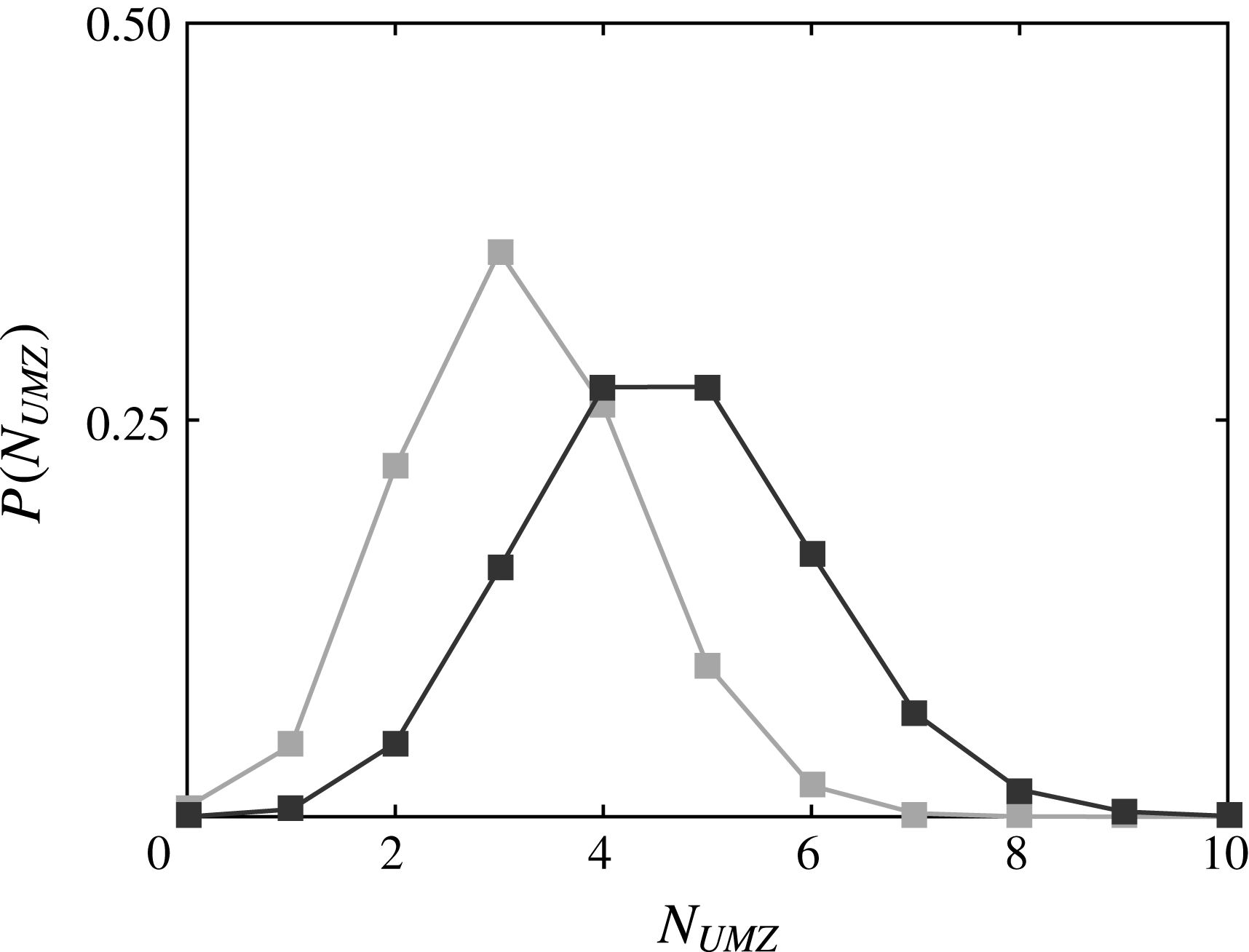
2600 viscous units). The removal of short-lived peaks leads to a significant decrease in the total number of peaks, without, however, altering the overall evolution of the number of zones. This can be seen in the PDF of
 $N_{UMZ}$
after removal of short-lived peaks (figure 5, grey symbols), which is centred around an average of 3.2 peaks.
The PDF of
 $N_{UMZ}$
, for all detected peaks (black symbols) and considering time-coherent peaks only (grey symbols).

In the following sections, the geometric characteristics of time-coherent UMZs and associated flow statistics are discussed in detail. It should be noted that this analysis was also performed for snapshot UMZs (i.e. before applying temporal threshold); while we feel the temporal filter more accurately represents the physics, the snapshot approach acts as a benchmark for comparison to earlier studies without time-resolved data. Appendix B discusses the results of the snapshot approach where they differ from the time-coherent approach.
4 Characteristics of time-coherent uniform momentum zones
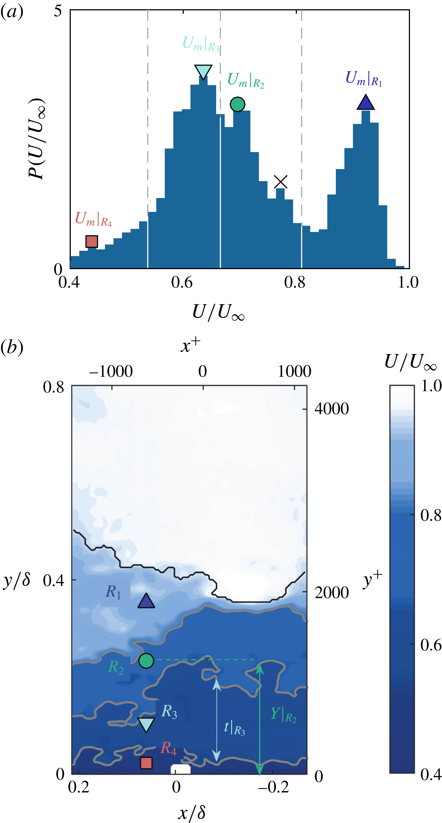
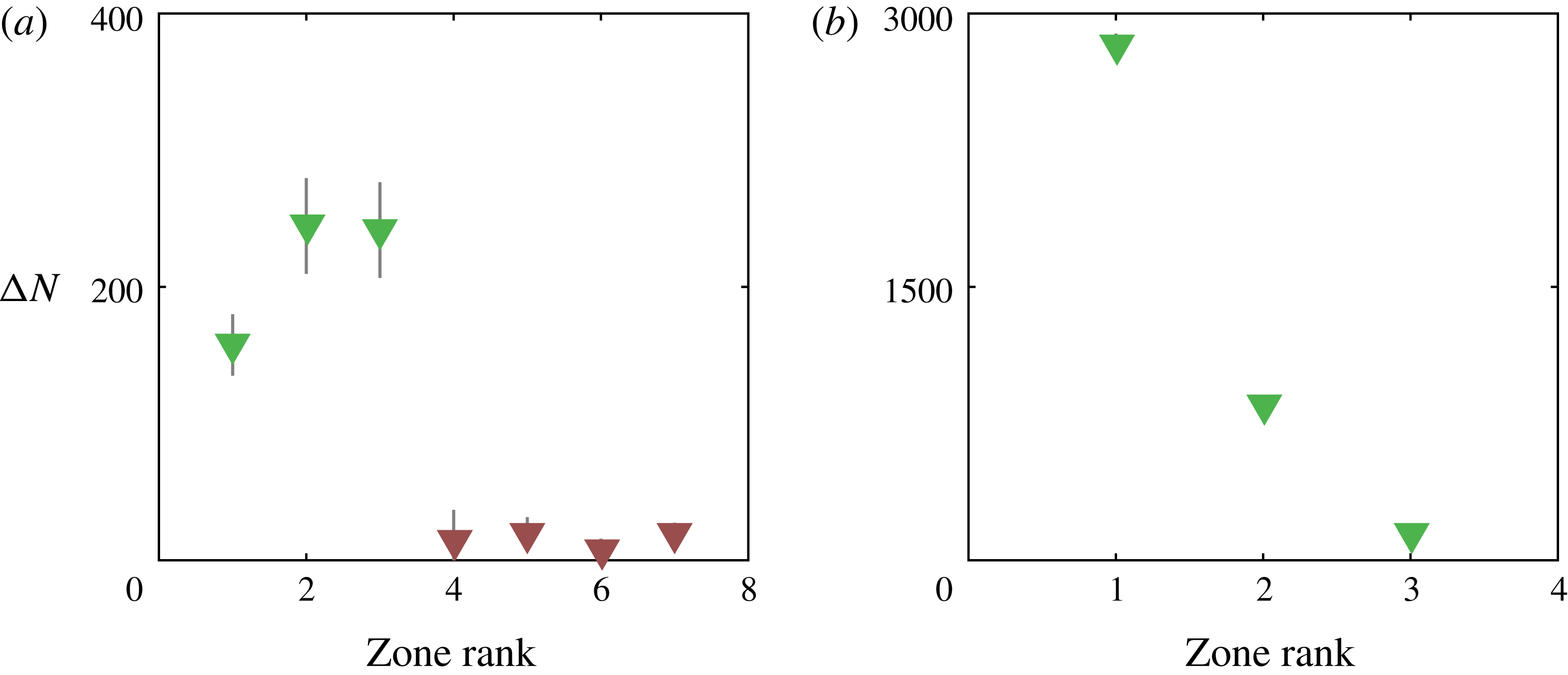
Classification system based on zone rank. The zone closest to the freestream is defined as rank one (blue triangle,
 $R_{1}$
) while the others below it follow in ascending order. (a) The pdf of
 $U/U_{\infty }$
for an instantaneous velocity field with
 $N_{UMZ}=4$
. Grey dashed lines mark the internal layers that distinguish the different UMZs and the modal velocity of each zone
 ${U_{m}|}_{R_{j}}$
, is marked with coloured symbols according to rank.
 $\times$
symbol denotes an instantaneously detected, short-lived peak that was discarded. (b) Velocity contours of the same velocity snapshot as in (a). Grey solid lines denote the boundaries of each zone while the TNTI is marked with black.

After detecting all UMZs and removing short-lived ones, statistical results of their main characteristics are presented in this section. These include the modal velocity associated with each UMZ,
 $U_{m}$
, the wall-normal location,
 $Y_{R_{j}}$
, and thickness,
 $t_{R_{j}}$
, of each zone. They are schematically shown in figure 6 for a single velocity snapshot. The thickness of the UMZs is defined as the average difference between the upper and lower boundary of each zone, while the wall-normal location is defined as the distance from the wall of the midpoint between the two boundaries.
Due to the large amount of data available and in order to represent these results in a clear fashion, a grouping of the UMZs is necessary. Two classification systems will be presented here. The first one, following de Silva et al. (Reference de Silva, Hutchins and Marusic2016), involves grouping all UMZs based on the inner-normalised momentum deficit of their associated modal velocities,
 $U_{MD}^{+}=(U_{\infty }-U_{m})/U_{\unicode[STIX]{x1D70F}}$
. Three different groups are defined, with
 $U_{MD_{1}}^{+}\in \,[0,6)$
for the first group and the one closest to the free stream,
 $U_{MD_{2}}^{+}\in [6,12)$
for the intermediate and
 $U_{MD_{3}}^{+}\in (12,18]$
for the third group that includes the zones closest to the wall. The subscript
 $MD_{i}$
will be used in the rest of the section to refer to this system, with
 $i=1,2,3$
denoting each group respectively. This classification distinguishes between zones closer to the wall (where the corresponding momentum deficit is high) and zones closer to the free stream (low momentum deficit levels). However, UMZs that are detected in the same snapshot and belong to the same momentum deficit class, might still exhibit different characteristics. For this reason, we introduce a second classification scheme, in which the number of groups, termed ‘ranks’, is equal to the number of UMZs present in each snapshot,
 $N_{UMZ}$
. This means that a snapshot with
 $N_{UMZ}=4$
, will also have 4 ranks (a representative illustration of this case can be seen in figure 6). The UMZ with the highest modal velocity in each snapshot belongs to the first rank and all others follow in ranks of ascending order, based on their modal velocity. The zone with the lowest modal velocity in each snapshot belongs to the last rank, equal to
 $N_{UMZ}$
. It then follows that the total number of ranks will be equal to the maximum
 $N_{UMZ}$
from all snapshots, which for time-coherent UMZs is
 $N_{UMZ}=8$
. Due to insufficient statistical convergence for the last two ranks (
 $N_{UMZ}=7$
and
 $8$
, see also figure 5), only the first six will be considered here. The subscript
 $R_{j}$
will be used to refer to this system, with
 $j=1,\ldots ,6$
denoting each rank. An example of how different zone ranks evolve in time can be found in the supplementary material (supplementary movie 2).
After all UMZs have been classified, their main characteristics are presented in the next subsections, for all groups of the two classification schemes. The influence of
 $N_{UMZ}$
on both the zones’ characteristics and the flow statistics is also discussed.
4.1 Modal velocity
The mean value and distribution of
 $U_{m}$
and their dependence on
 $N_{UMZ}$
are presented here, for all groups of the two classification systems described above.
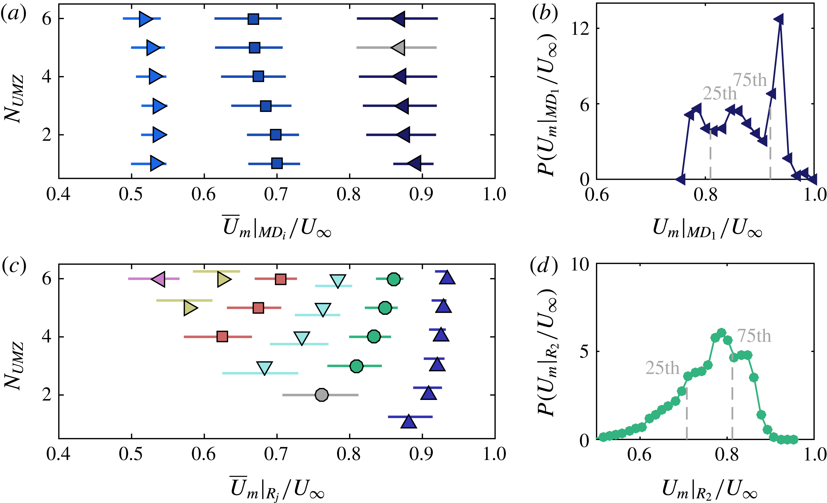
Modal velocities for the two classification systems and their dependence on
 $N_{UMZ}$
. (a,b) Classification based on momentum deficit,
 $U_{MD}^{+}$
. Modal velocities,
 ${U_{m}|}_{MD_{i}}$
for three momentum deficit groups:
 $U_{MD_{1}}^{+}\in [0,6)$
(◀ ),
 $U_{MD_{2}}^{+}\in (6,12]$
(▪),
 $U_{MD_{3}}^{+}\in (12,18]$
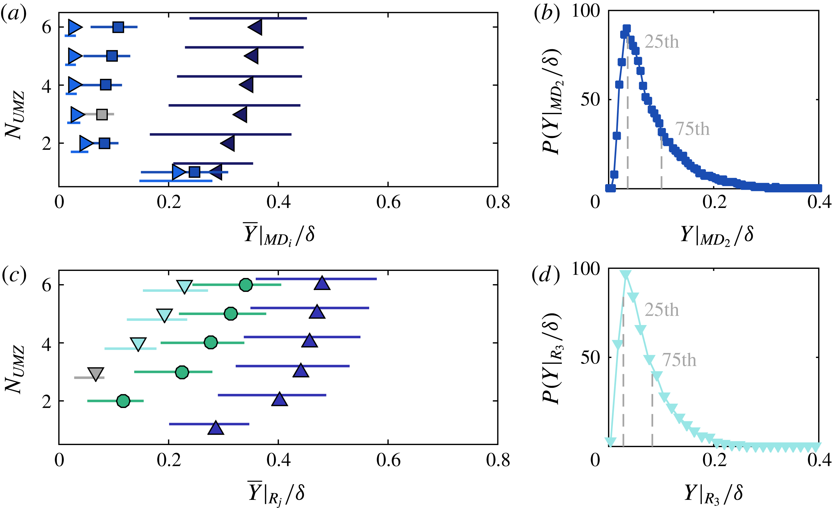
( ▶). Symbols denote mean values and solid lines the pdf extent between the 25th and 75th percentile (grey dashed lines on subfigure b). Grey coloured symbols denote the mean and extent of the example pdf shown in (b). UMZs with low momentum deficit (◀ ) show little variation with increasing
 $N_{UMZ}$
, while the group of the largest deficit ( ▶) moves to lower modal velocities as new zones appear close to the wall. (c,d) Classification based on zone rank. Modal velocities,
 ${U_{m}|}_{R}$
, for six zone ranks. Symbols as in figure 6. All ranks move to higher modal velocities as
 $N_{UMZ}$
increases.

For the first classification system (figure 7
a,b), based on the momentum deficit level of each zone, three different groups are defined, as was mentioned above. The first group with
 $U_{MD_{1}}^{+}\in [0,6)$
, includes the zones closest to the free stream. The average modal velocity,
 ${\overline{U}_{m}|}_{MD_{1}}$
(◀ in figure 7
a) of zones belonging to that group, and the spread around it (solid lines in figure 7
a), show virtually no change as
 $N_{UMZ}$
varies. This suggests that as
 $N_{UMZ}$
increases and more zones appear, the group of UMZs with low
 $U_{MD}^{+}$
remains largely unaltered. An example PDF of
 $U_{m}$
for zones belonging to this group when
 $N_{UMZ}=5$
, can be seen in figure 7(b) (some slight pixel-locking effects can still be seen in this figure that amplify the prominent modal velocities). The groups of intermediate (
 $U_{MD_{2}}^{+}\in [6,12)$
, squares in figure 7
a) and large (
 $U_{MD_{3}}^{+}\in [12,18)$
, ▶ in figure 7
a) momentum deficit levels show a slight decrease in the average modal velocity as
 $N_{UMZ}$
increases, while the distribution around that mean becomes wider. This behaviour indicates that, when
 $N_{UMZ}$
increases, the newest zones appear near the wall and therefore contribute to the classes of intermediate or large momentum deficit, while the class of zones closest to the free stream remains unaltered. In snapshots where only one zone is present (
 $N_{UMZ}=1$
), the momentum deficit of that single UMZ is still classified to either of the aforementioned groups. As can be seen in figure 7(a), all three groups are represented, suggesting that single UMZs could have
 $U_{MD}^{+}$
values ranging from 0 to 18. What is, however, not apparent is that, statistically, single UMZs tend to have low momentum deficit levels and mostly contribute to the first group (
 $U_{MD_{1}}^{+}\in [0,6)$
). As
 $N_{UMZ}$
increases and new zones appear at the wall, the other two groups become increasingly populated.
This process is clearer when the zones are classified based on their rank (figure 7
c,d). Here, the first group ( ▲ in figure 7
c), includes UMZs that have the largest modal velocity in each snapshot. When
 $N_{UMZ}=1$
, all single UMZs contribute only to that first group and it is now apparent that most of them have modal velocities close to the free stream, albeit with some significant variation (solid lines in figure 7
c), as was mentioned above. More generally for low
 $N_{UMZ}$
, all groups have modal velocities close to
 $U_{\infty }$
, with wide distributions, mostly skewed towards the free stream (a representative example can be seen in figure 7
d). As
 $N_{UMZ}$
increases, the mean modal velocities of all ranks are shown to move to higher values, while the spread around them becomes progressively narrower. Zones of higher rank, that are closer to the wall, show the largest modal velocity increase with increasing
 $N_{UMZ}$
, while the ones close to the free stream exhibit only a marginal rise. This supports the observations from the first classification scheme, where new zones were shown to appear near the wall and influence the group of the largest momentum deficit. It should also be noted here that, the appearance of newer zones of larger momentum deficit, close to the wall, is in agreement with the attached eddy model, which assumes that the origin of the vortical structures populating the boundary layer is at the wall (see Head & Bandyopadhyay Reference Head and Bandyopadhyay1981 and Perry & Chong Reference Perry and Chong1982).
4.2 Wall-normal location and thickness
Apart from the modal velocity, the UMZs of each group are characterised in physical space by their average wall-normal location,
 $\overline{Y}$
and thickness,
 $\overline{t}$
(see figure 6).
When the zones are classified based on their momentum deficit level (figures 8
a,b), the first group, with the lowest momentum deficit (◀ in figure 8
a), is at the largest distance from the wall and shows the largest variation in wall-normal location with
 $N_{UMZ}$
. More specifically, as
 $N_{UMZ}$
increases, the zones belonging to that group move further towards the free stream, to accommodate the new ones that appear near the wall. On the other hand, the group of zones with the largest momentum deficit ( ▶ in figure 8
a), is the one closest to the wall, and as
 $N_{UMZ}$
increases and the group becomes more populated, its average wall-normal location decreases further. This means that, although existing zones will tend to move outwards to accommodate the new ones appearing at the wall, the dominant factor in this group, as
 $N_{UMZ}$
increases, is the lower wall-normal location of the new zones that appear closer to the wall. It should also be noted here that, as was mentioned above, when
 $N_{UMZ}=1$
, most of the single UMZs belong to the first group, with the lowest momentum deficit. This however, leads to convergence issues for the statistics of the other two groups, reflected in the large deviations observed in
 $\overline{Y}|_{MD_{2}}$
and
 $\overline{Y}|_{MD_{3}}$
(figure 8
a), when
 $N_{UMZ}=1$
.
Wall-normal locations for the two classification systems and their dependence on
 $N_{UMZ}$
. Colours and symbols as in figure 7. (a,b) Wall-normal locations,
 $Y|_{MD_{i}}$
, for a classification based on momentum deficit. For an increase in
 $N_{UMZ}$
, the zones with the lowest momentum deficit (◀ ) move to higher wall-normal locations, to account for the newest ones that appear near the wall. (c,d) Wall-normal locations,
 $Y|_{R_{j}}$
, for a classification based on zone rank. Only the first three ranks are shown for clarity, however the trend is similar for all following ranks. All ranks move upwards while new zones of higher rank appear below them.

When the zones are classified based on their rank (figure 8
c,d), there is a monotonic increase in wall-normal location for zones of all ranks. This supports the observation that as
 $N_{UMZ}$
increases and zones of higher rank appear closer to the wall, existing UMZs of lower rank with higher modal velocities will move further away from the wall to accommodate for the new ones.
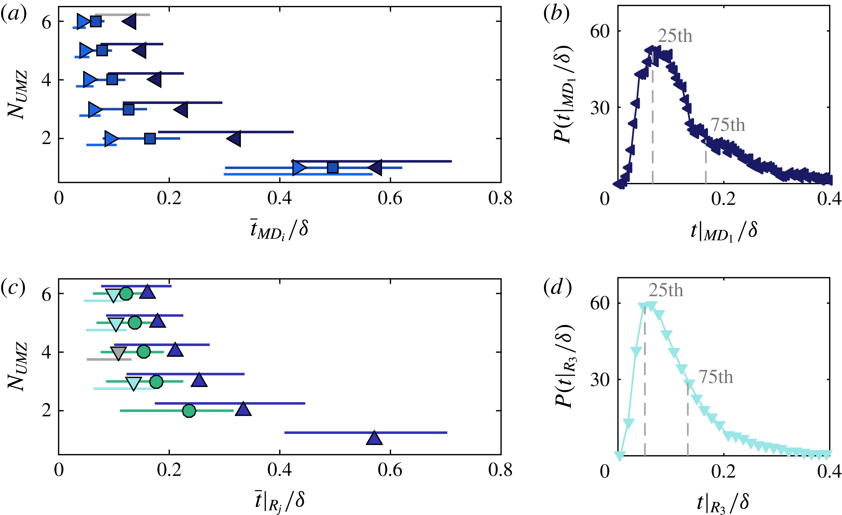
The mean thickness of the different UMZs (see figure 6
b for a schematic definition) is also presented for the two different classification systems (figure 9). When the zones are classified according to their momentum deficit level and in line with the observations from de Silva et al. (Reference de Silva, Hutchins and Marusic2016), the average thickness is higher for groups of zones with low momentum deficit levels and the distribution around that average is wider (figure 9
a,b). The mean thickness of all the groups and the fluctuations around it show a decreasing trend with increasing number of zones. Here again, the large values and wide distributions for
 $\overline{t}|_{MD_{2}}$
and
 $\overline{t}|_{MD_{3}}$
when
 $N_{UMZ}=1$
(figure 9
a), are due to poor convergence for these two groups when only one UMZ is present in our FOV.
A very similar behaviour of decreasing zone thickness when
 $N_{UMZ}$
increases, can also be seen when the zones are classified according to their rank (figure 9
c,d). An increasing number of zones, will compress the thickness of all the zones, although their wall-normal position will increase (figure 8
c,d).
Zone thickness for the two classification systems and its dependence on
 $N_{UMZ}$
. Colours and symbols as in figure 7. (a,b) Zone thickness,
 $t|_{MD}$
, for a classification based on momentum deficit. (c,d) Zone thickness,
 $t|_{R}$
, for a classification based on zone rank. Only the first three ranks are shown for clarity, however the trend is similar for all following ranks. Both systems show similar trends of decreasing thickness with increasing
 $N_{UMZ}$
. Zones closer to the wall have shorter wall-normal extent on average and a much narrower distribution around it.

4.3 Total number of zones
Based on the observations of the previous section, the total number of zones present in a given snapshot is a critical factor influencing UMZ characteristics. This influence could possibly indicate further structural differences of the flow, so here we present some basic statistical properties of the flow when conditioned on
 $N_{UMZ}$
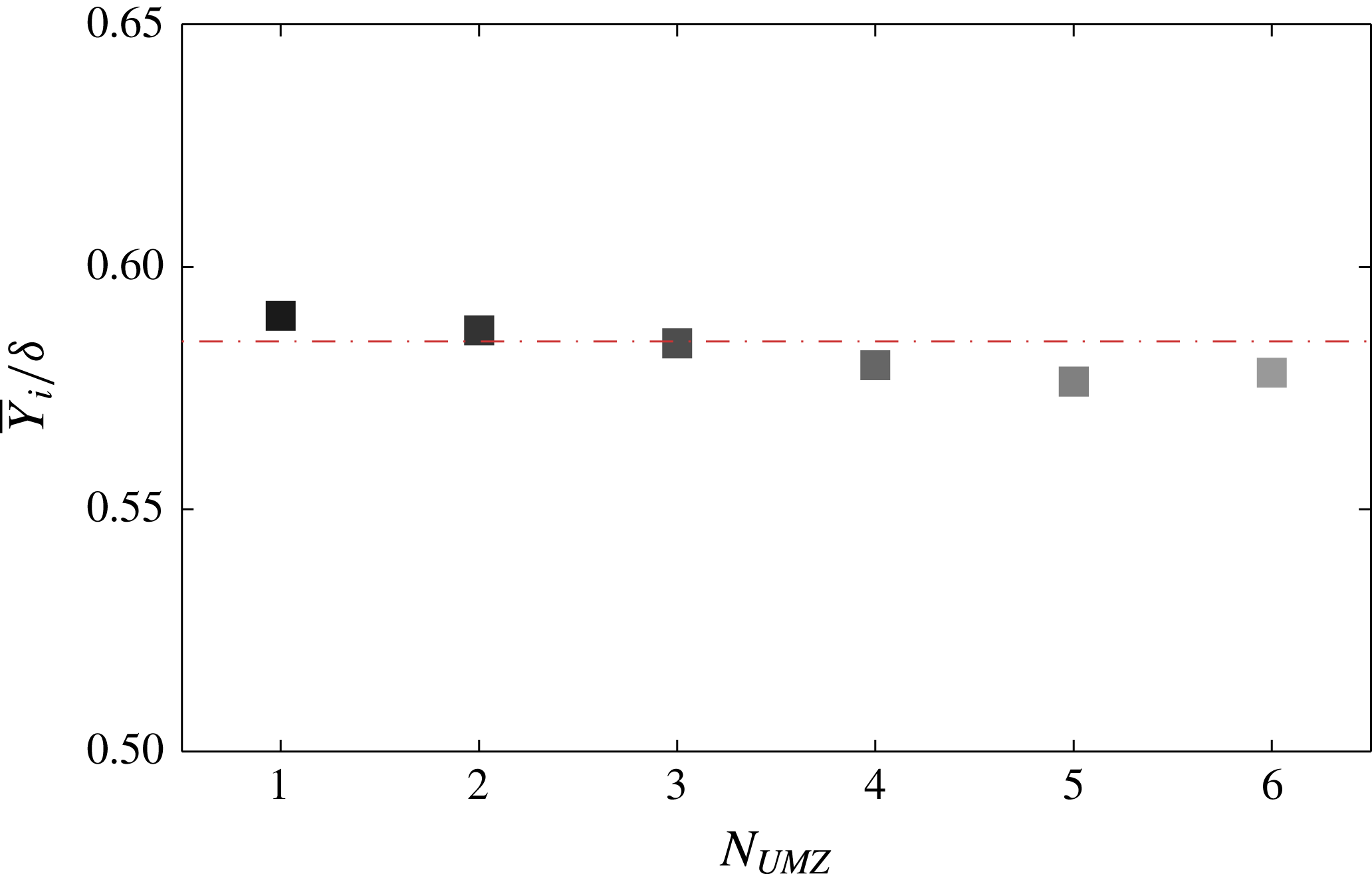
. As mentioned above, when the total number of zones increases, the thickness of all zones decreases, while their average wall-normal position increases. The combination of these two trends results in an almost constant TNTI, with only a slight decrease for an increasing
 $N_{UMZ}$
(figure 10). This is also the most notable difference we found between instantaneously detected and time-coherent peaks. More specifically, when all modal peaks are considered, and no temporal threshold is applied, the thickness of all zones still follows a decreasing trend for an increasing
 $N_{UMZ}$
however, their wall-normal position decreases as well. That leads to significantly lower TNTI location for a high number of zones (see appendix B for a more detailed discussion).
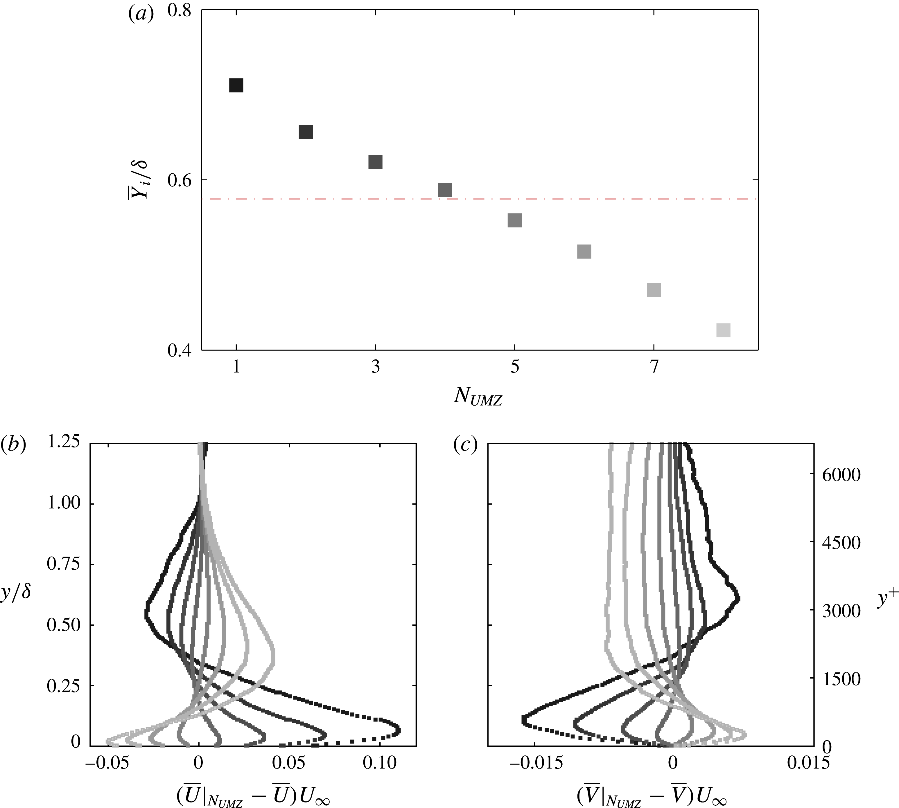
Variation of the mean location of the TNTI,
 $\overline{Y}_{i}$
, with the number of UMZs detected. Colour gradient from dark to light denotes increasing number of zones. Red dotted line denotes the global average location of the TNTI.

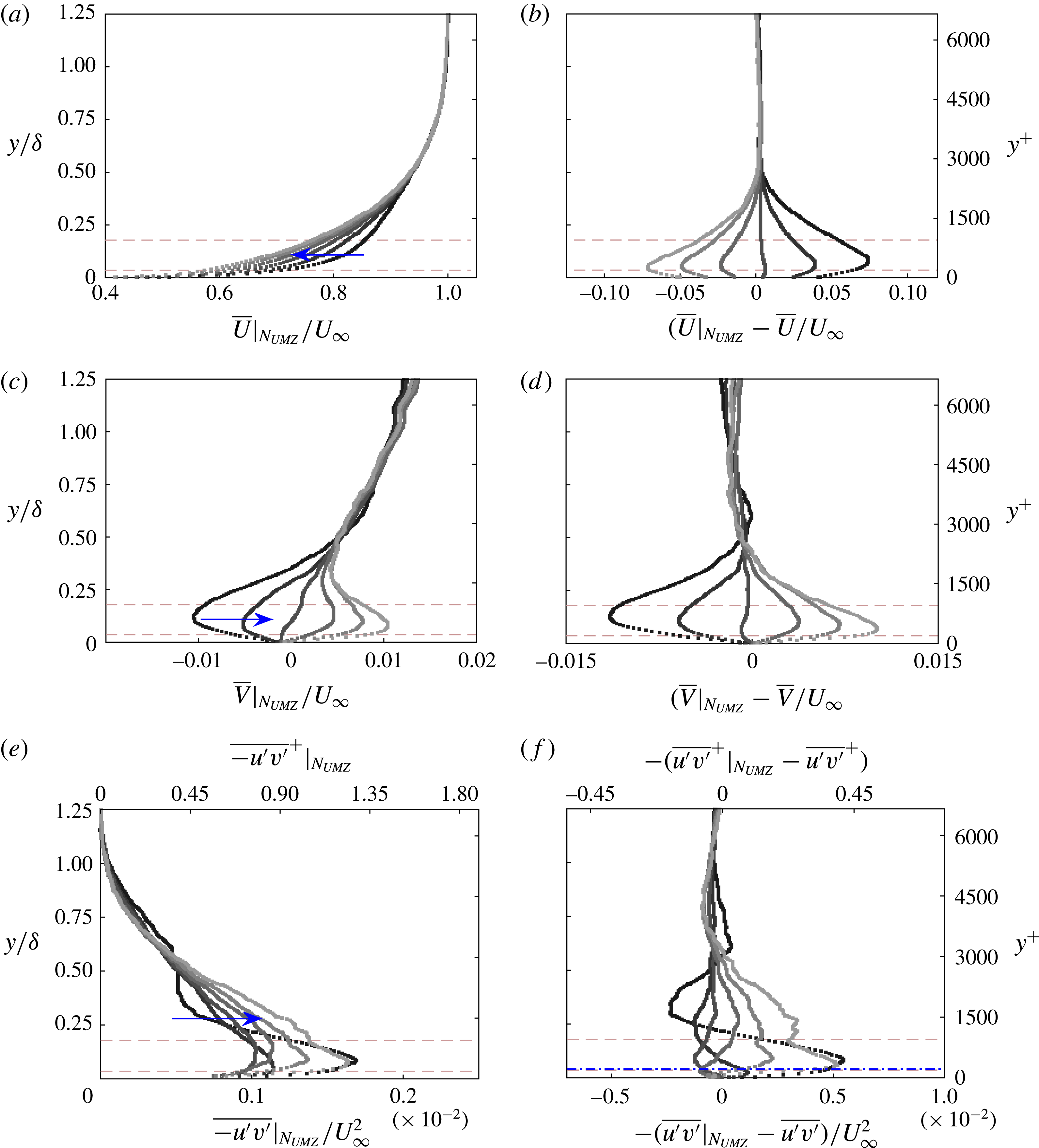
Conditionally averaged statistics with varying
 $N_{UMZ}$
. Blue arrows and lighter greyscales indicate increasing number of zones (from 1 to 6). Dashed lines denote the limits of the logarithmic region based on the global time-averaged streamwise velocity (see figure 1
a). (a) Outer-normalised mean streamwise velocity profile. (b) Difference from the global streamwise average,
 $\overline{U}$
. (c) Outer-normalised mean wall-normal velocity profile. (d) Difference from the global wall-normal average,
 $\overline{V}$
. (e) Root-mean-squared profile of the Reynolds shear stress. (f) Difference from the global Reynolds shear stress profile,
 $\overline{u^{\prime }v^{\prime }}$
. Blue dash-dot lines indicate the cross-over point.

Apart from the TNTI location, flow statistics also show a strong dependence on
 $N_{UMZ}$
. A large number of zones leads to a strong momentum deficit in the region near the wall (
 $y<0.25\unicode[STIX]{x1D6FF}$
) (figure 11
a,b). This is in line with the conclusions from the previous section, where it was shown that an increasing number of zones leads to a decrease of the mean modal velocity of the lower UMZs (figure 7
b), because new zones tend to appear closer to the wall therefore adding to the momentum deficit in that region. At the same time, within that region, the vertical velocity component is shown to be significantly increased compared to the global average,
 $\overline{V}$
(figure 11
c,d). This combined behaviour of
 $U$
and
 $V$
statistics indicates a large-scale
 $Q2$
event in the log region for a high
 $N_{UMZ}$
. When
 $N_{UMZ}$
is low, the opposite trends are observed in both the streamwise and the wall-normal velocity profiles. Close to the wall there is a strong downward motion (figures 11
c,d), pushing high-speed fluid to regions of lower momentum, thus creating a slight increase of
 $U$
, reflected in a fuller streamwise velocity profile when compared to the global average,
 $\overline{U}$
(figures 11
a,b). These two trends suggest the presence of a large-scale
 $Q4$
event in the log region for a low
 $N_{UMZ}$
. The region closer to the free stream shows no significant variation, in line with the almost constant average TNTI location (figure 10). It should also be noted here that from all profiles presented, the profile representing
 $N_{UMZ}=3$
(third profile from the right in figure 11), is averaged over the largest fraction of velocity snapshots (see also PDF in figure 5) and as such is the one closest to the global average.
Finally, conditional averages of the Reynolds shear stress profiles show that closer to the wall, there is increased turbulent activity when compared to the global average for low
 $N_{UMZ}$
, which then rapidly decreases and only slightly re-surges close to the free stream. In contrast, a high
 $N_{UMZ}$
is coupled with low turbulent activity very close to the wall, which then significantly increases in the logarithmic region and gradually reaches the global average farther away from the wall. This behaviour can potentially be linked with previously documented small-scale activity when conditioned to a large-scale log-layer structure (amplitude modulation). More specifically, Hutchins & Marusic (Reference Hutchins and Marusic2007b
) showed that the presence of large-scale high-speed events (‘superstructures’) in the logarithmic layer (corresponding to an outer spectral peak
 ${\approx}6\unicode[STIX]{x1D6FF}$
), creates an increase of small-scale activity very close to the wall, while low-speed log structures have the opposite effect. They further noticed that this behaviour is reversed after a certain distance from the wall (termed the ‘cross-over’ point) and that this point of reversal is Reynolds number dependent. Later, Mathis, Hutchins & Marusic (Reference Mathis, Hutchins and Marusic2009) supported this observation and proposed that the point where the correlation between the large-scale component with the envelope of the small-scale component crosses zero, happens within the logarithmic region, at an estimated
 $y_{c}^{+}\propto \sqrt{Re_{\unicode[STIX]{x1D70F}}}$
(blue dash-dot line in figure 11(f), located at
 $0.04\unicode[STIX]{x1D6FF}$
in the present data), an estimation also supported by Ganapathisubramani et al. (Reference Ganapathisubramani, Hutchins, Monty, Chung and Marusic2012). Similar results were presented by Dennis & Nickels (Reference Dennis and Nickels2011), who showed that increased Reynolds shear stress regions were correlated with long low-speed structures while the high-speed ones did not exhibit a similar correlation.
In the present case, when the number of zones is low, there is a significant increase of streamwise momentum in the log region that could signify the passage of high-speed structures. Following the amplitude modulation reasoning and noting that the majority of the available vectors are above the cross-over point (blue dash-dot line in figure 11
f), this would lead to a decrease in the amplitude of the small scales, as is indeed observed in the Reynolds shear stress profile (the only notable exception being the case of
 $N_{UMZ}=1$
for which a decrease in amplitude is observed outside of the log region). Below the cross-over point the situation reverses and the passage of a high-speed structure in the log region is expected to amplify small-scale activity. The current resolution does not provide sufficient data of that region, however it is possible that new zones are created there that are not detected using the available vectors. Conversely, when the number of zones is high, the log region is characterised by a significant momentum deficit, which in turn can be linked to low-speed structures and increased small-scale activity would be expected. Results again support this argument, with the Reynolds shear stress values being significantly increased compared to global average, when a large number of zones is present in the flow (figure 11
f).
4.4 Large-scale
 $Q2$
and
$Q4$
events in the log region


The above discussion on amplitude modulation is based on the assumption that the observed large-scale
 $Q2$
(
 $Q4$
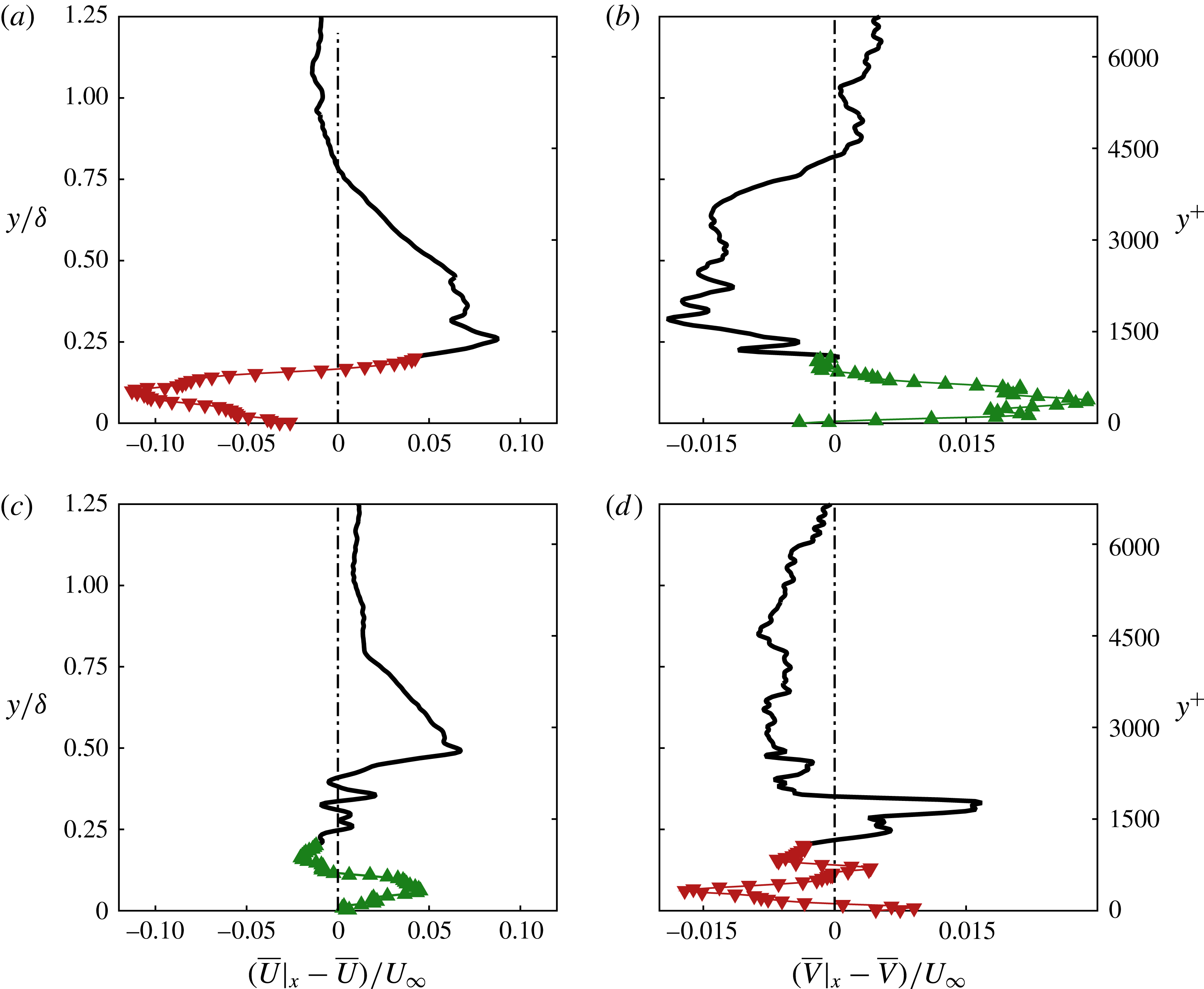
) events in the log region indicate the passage of low- (high)-speed structures that have a substantial coherence in space. Since the available velocity snapshots are time resolved, the time for which such events reside within our FOV can be computed and their spatial extent can be subsequently estimated. In order to assess this concept we first classify all available snapshots based on whether they match the resulting profiles on figure 11(b,d). More specifically, for every velocity snapshot, the deviation, in the log layer, of the
 $\overline{U}|_{x}$
and
 $\overline{V}|_{x}$
velocity profiles (averaged across the streamwise extent of the FOV) from the global means,
 $\overline{U}$
and
 $\overline{V}$
, is estimated. The signed integral between the resulting profiles (see figure 12) and the
 $y$
-axis is the basis of our definition for the log-layer events. We define as a large-scale
 $Q2$
event a combination of a negative integral
 $\overline{U}|_{x}-\overline{U}$
value and a positive integral
 $\overline{V}|_{x}-\overline{V}$
value, in the log region (a representative example is depicted on figure 12
a,b). The opposite behaviour (figure 12
c,d) is classified as a
 $Q4$
event. Overall, such events are found to account for
 $74\,\%$
of all instantaneous fields. This is in line with the results on three-dimensional structures in a turbulent boundary layer by Dennis & Nickels (Reference Dennis and Nickels2011), who documented a high correlation of increased streamwise momentum with a downwards motion and a momentum deficit region with an upwards movement.
It should be noted here that this definition of
 $Q2$
and
 $Q4$
events differs from the standard quadrant analysis in that we do not classify the events based on pointwise velocity fluctuations, but rather on Reynolds shear stress values averaged over the size of our FOV. In that sense a large-scale
 $Q2$
(
 $Q4$
) event as defined here, would indicate an average ejecting (sweeping) motion for an area covering the whole streamwise extent and up to the end of the log region in the wall-normal direction. However, individual vectors within that area could still be classified in either of the four quadrants based on pointwise Reynolds shear stress.
Streamwise-averaged velocity profiles for two different snapshots representing a large-scale
 $Q2$
(a,b) and
 $Q4$
(c,d) event at the log region. ▼ Denote average velocity values in the log region lower than the global average and ▲ average velocity values in the log region higher than the global average.

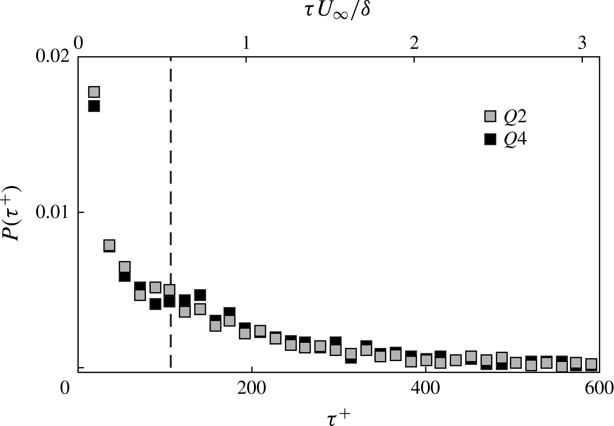
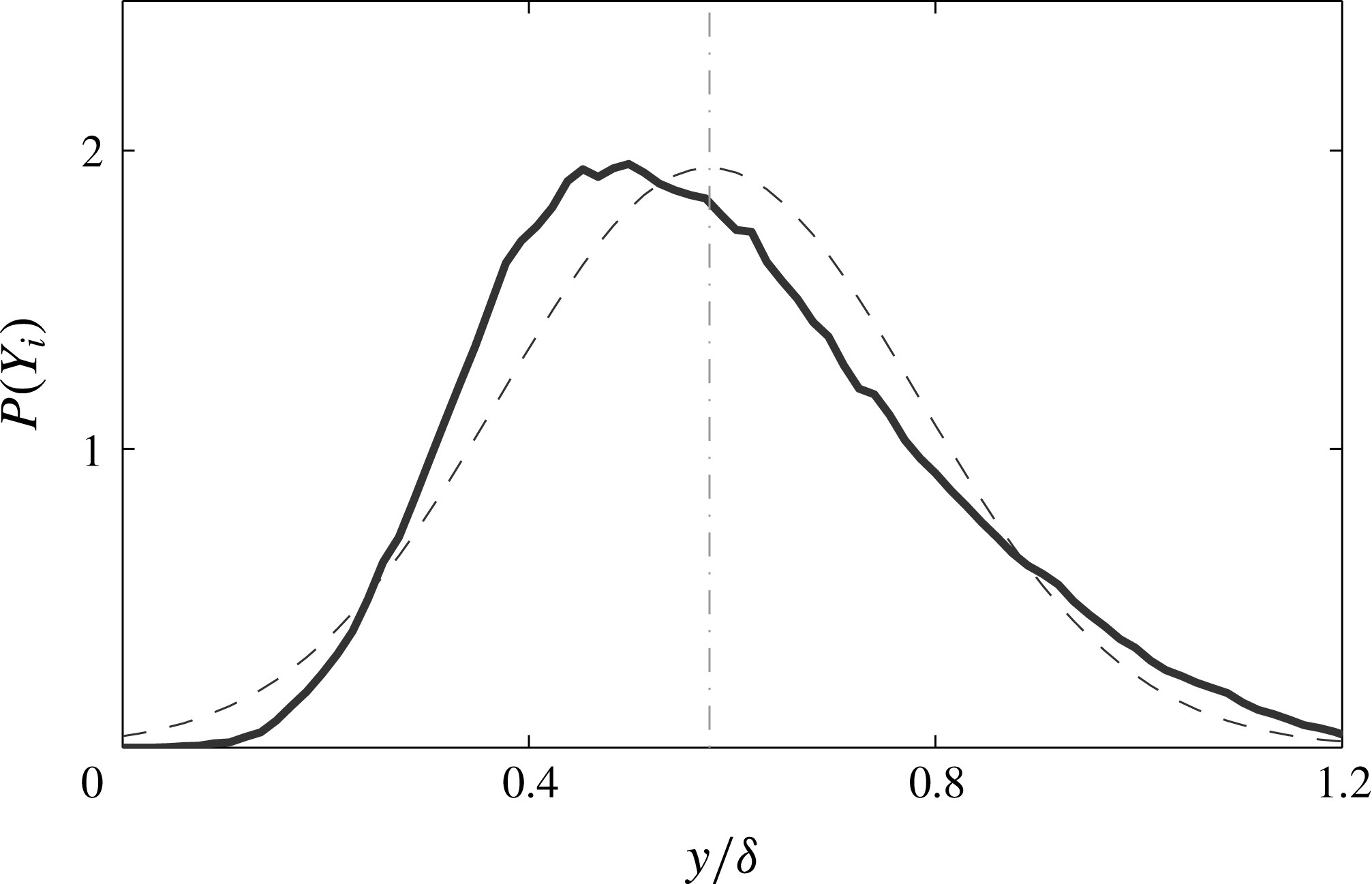
The PDF of residence times within the FOV for large-scale
 $Q2$
and
 $Q4$
events. Dashed lines denote the average residence times for both event types.

The resulting residence times (figure 13), show that on average, these profiles persist for
 $0.5\unicode[STIX]{x1D6FF}/U_{\infty }$
within the measurement domain (for both
 $Q2$
and
 $Q4$
events, dashed lines in figure 13) and the longest of them reach times of
 $3\unicode[STIX]{x1D6FF}/U_{\infty }$
(maximum recorded event of
 $6\unicode[STIX]{x1D6FF}/U_{\infty }$
). It should be stressed here that the profiles in figure 12 are a result of streamwise averaging and therefore indicate that the events considered are at least
 $0.5\unicode[STIX]{x1D6FF}$
long. Assuming moreover that the events move with approximately the local mean velocity (temporal mean at a wall-normal location of
 $y=0.1\unicode[STIX]{x1D6FF}$
for each event), the average time scales found indicate high-speed structures that are at least
 $0.9\unicode[STIX]{x1D6FF}$
long while low-speed ones are at least
 $0.8\unicode[STIX]{x1D6FF}$
long. While such an assumption on the convection velocities has long been disputed (see Fisher & Davies Reference Fisher and Davies1964; Zaman & Hussain Reference Zaman and Hussain1981; Kim & Hussain Reference Kim and Hussain1993; Davoust & Jacquin Reference Davoust and Jacquin2011, among others), recently, Geng et al. (Reference Geng, He, Wang, Xu, Lozano-Durán and Wallace2015) showed that in the logarithmic region of turbulent boundary layers, which is of interest here, the use of the streamwise mean as the convection velocity is a very good approximation. The maximum recorded residence times suggest the passage of structures of up to
 $6\unicode[STIX]{x1D6FF}$
, in line with reported scales of large-scale motions and superstructures in the logarithmic layer (see Ganapathisubramani et al.
Reference Ganapathisubramani, Longmire and Marusic2003; Tomkins & Adrian Reference Tomkins and Adrian2005; Hutchins & Marusic Reference Hutchins and Marusic2007b
; Dennis & Nickels Reference Dennis and Nickels2011, among others). On average however, both
 $Q2$
and
 $Q4$
events have similar but significantly shorter spatial extents. The main reason behind this is the much shorter temporal coherence of the vertical velocity
 $V$
when compared to the streamwise one. The reported long scales in the literature mainly refer to low or high streamwise velocity structures. In the present data, when only a high or low
 $U$
velocity event is tracked in time, the resulting residence times have a similar distribution to the
 $Q2$
and
 $Q4$
events (figure 13), but are on average twice as long (
 $1.2\unicode[STIX]{x1D6FF}/U_{\infty }$
), suggesting spatial extents closer to the documented values, albeit still shorter. Another reason for this is that our measurement domain is a streamwise wall-normal plane and that very long high and low momentum structures have been shown to alternate in the log region while also exhibiting a meandering motion in the spanwise direction (Hutchins & Marusic Reference Hutchins and Marusic2007a
,Reference Hutchins and Marusic
b
; Zheng & Longmire Reference Zheng and Longmire2014). Therefore, it can be argued that this presence of
 $Q2$
(
 $Q4$
) events, observed in the velocity profiles, signifies the passage of low (high) momentum structures through our field of view and their recorded time scale depends on their streamwise alignment with the measurement plane. A similar organisation of side-by-side
 $Q2$
and
 $Q4$
events in the logarithmic region of channels was also presented by Lozano-Duran, Flores & Jimenez (Reference Lozano-Duran, Flores and Jimenez2012), who showed that these events form a predominant structure which is completed by a vortex cluster primarily located within the
 $Q2$
event but extending slightly underneath the
 $Q4$
as well.
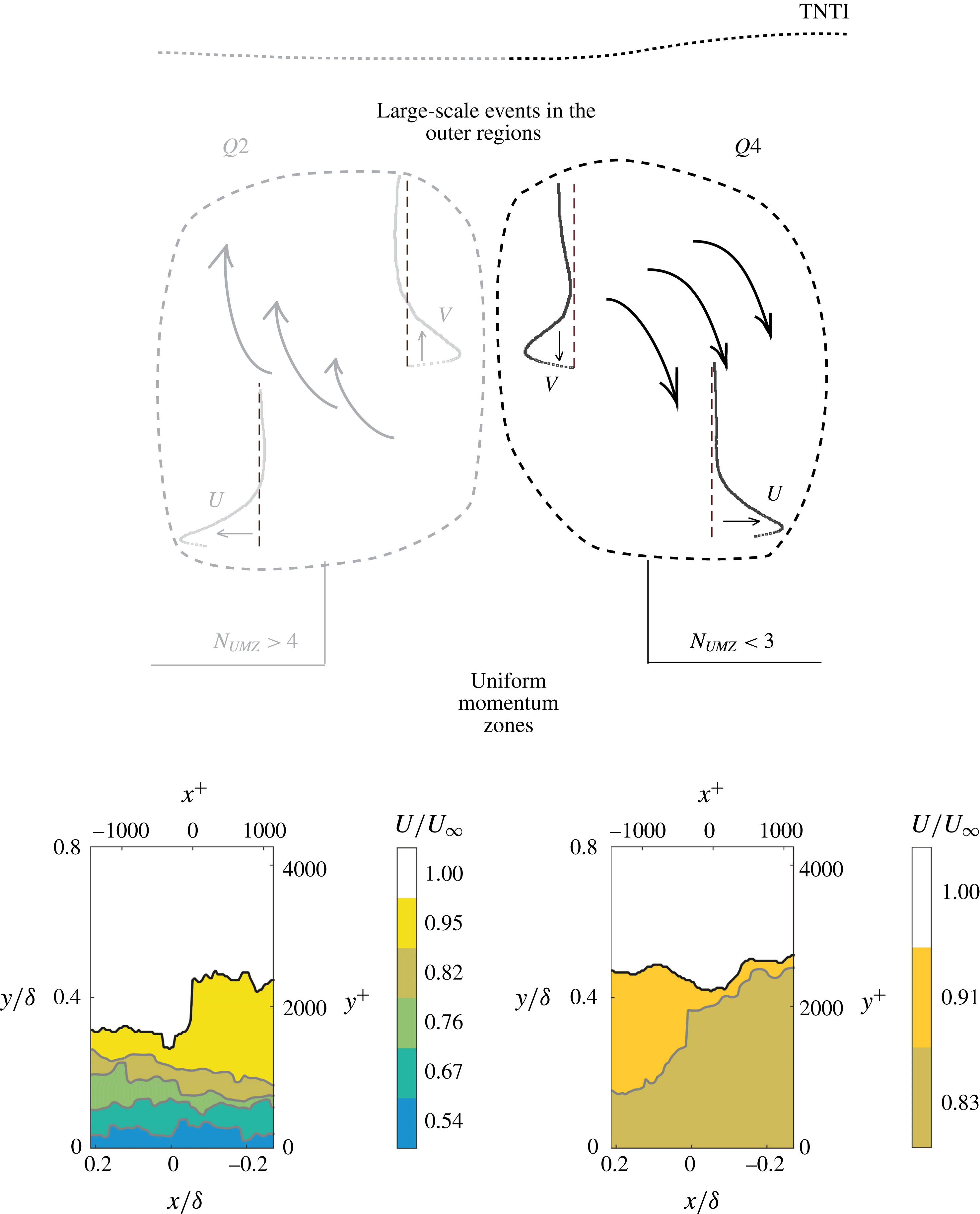
The conditionally averaged statistics presented above (figure 11), have shown that velocity profiles exhibit a large, sweep-like behaviour in the log region for cases of a low number of zones present in the flow, while large-scale ejection-like events dominate for high
 $N_{UMZ}$
. The TNTI location is shown to be almost constant when conditioned on the number of zones (figure 10) with only a slight decrease with increasing
 $N_{UMZ}$
, although this trend was much stronger for an instantaneous peak detection (appendix B). In order to further investigate the correlation between
 $N_{UMZ}$
,
 $\overline{Y}_{i}$
, and the presence of these high- or low-speed log structures, conditional averaging is used again. This time however, the latter two parameters are used as conditions, while the resulting variations in
 $N_{UMZ}$
are recorded.
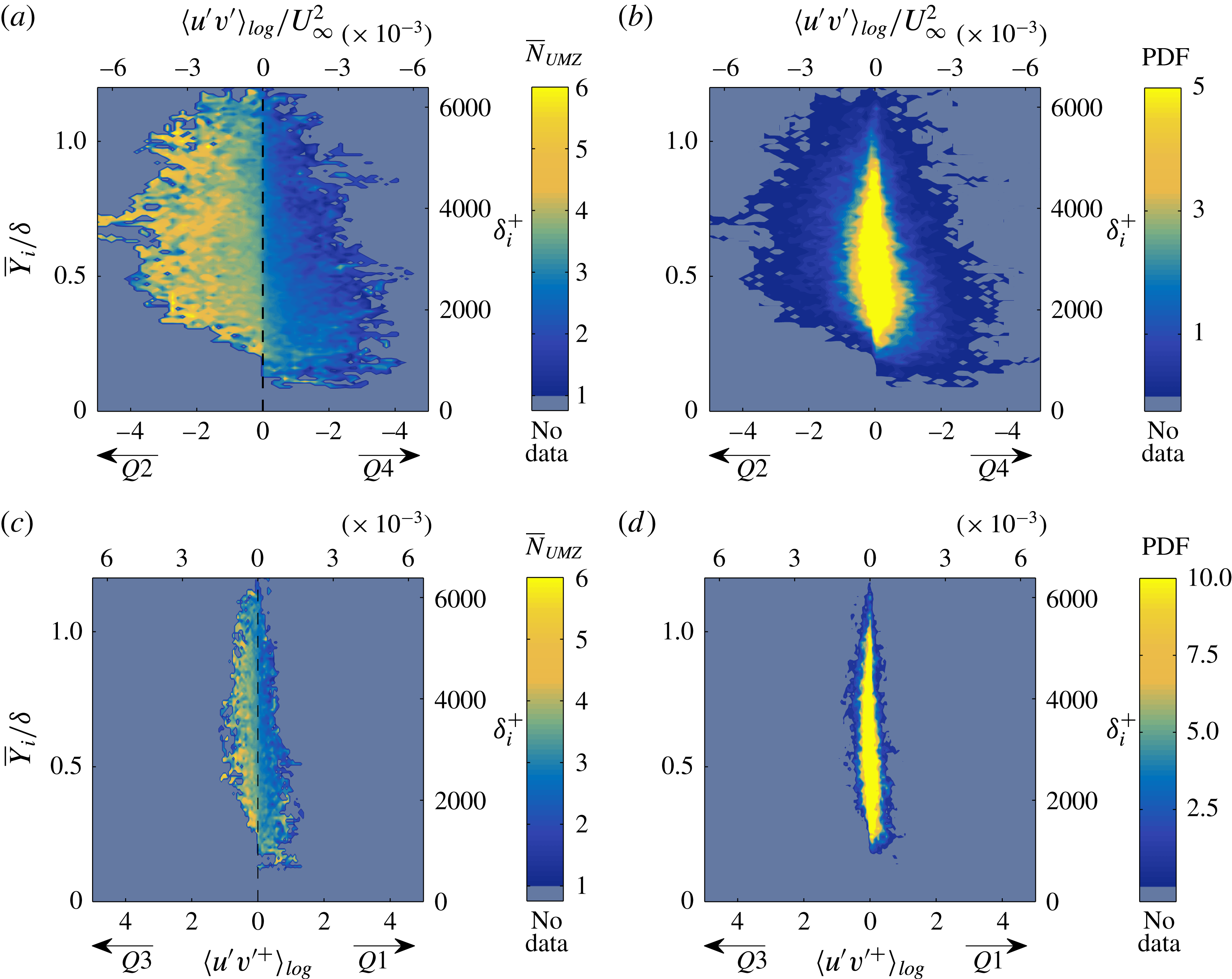
The PDF of the average number of zones present in the flow,
 $\overline{N}_{UMZ}$
, for varying TNTI location,
 $\overline{Y}_{i}$
and magnitude of log region events. Average number of zones (a) and PDF of realisations for large-scale
 $Q2$
,
 $Q4$
events in the log region (b). In total, they occur in
 $74\,\%$
of all cases. Average number of zones (c) and PDF of realisations (d) for large-scale
 $Q1$
,
 $Q3$
events in the log region (
 $26\,\%$
of all cases).

We follow the procedure discussed above to identity
 $Q2$
and
 $Q4$
events in the log region and we subsequently estimate their magnitude together with the instantaneous TNTI location in every snapshot. The joint PDF of these two parameters is computed, showing how many times a certain combination of events takes place (figure 14
b). The average number of zones over these realisations is subsequently estimated (figure 14
a) and the resulting map of
 $\overline{N}_{UMZ}$
shows that, indeed, a similar correlation as the one shown in figures 10 and 11 exists. More specifically, a
 $Q2$
event in the log layer results on average in a high number of zones (
 $\overline{N}_{UMZ}\geqslant 5$
), a number which tends to increase further with increasing ejection magnitude. The presence of a
 $Q4$
event on the other hand results in a low number of zones, in line with the conditional averages in figure 11. The TNTI location is again shown to have a limited effect on the resulting number of zones (see also figure 10). These results (figure 14
a,b), were based on the presence of either a
 $Q2$
- or
 $Q4$
-like large-scale event in the log region. Overall such events occur in
 $74\,\%$
of the total snapshots available and therefore the trends observed in figure 14(a,b) will be the ones dominating in a global sense. However, for completeness, a similar map of
 $\overline{N}_{UMZ}$
is presented for the other type of events, namely the
 $Q3$
(inward) and
 $Q1$
(outward) events (figure 14
c,d). The resulting PDFs show that these events are significantly weaker in magnitude and they mostly represent cases of average
 $N_{UMZ}$
. Even though there is no clear segregation of extremes like the one in figure 14(a) (instances with very low number of zones are almost non-existent), there is still a strong trend of increasing
 $\overline{N}_{UMZ}$
for low-speed structures present in the log region (
 $Q3$
events). Considering all quadrant events, an increase of the streamwise velocity is shown to be correlated with a decrease in the number of zones (
 $Q1$
and
 $Q4$
events), while a lower than average streamwise velocity has the opposite effect (
 $Q2$
and
 $Q3$
events). When the large-scale high-speed events are combined with a downwards motion there is a further decrease in the number of zones. Conversely, when the low-speed events are combined with an upwards motion (
 $Q2$
events), the number of zones increases further.
Finally, a comment should be made regarding the temporal coherence of the large-scale events in the log region and how it could affect the time scales of UMZs. As mentioned above, large-scale
 $Q2$
and
 $Q4$
events in the log layer that have average residence times of
 $0.5\unicode[STIX]{x1D6FF}/U_{\infty }$
, can potentially trigger the organisation of the flow into either low or high
 $N_{UMZ}$
, respectively. Individual UMZs however, represent flow regions that have an almost constant modal velocity, either higher or lower than the local mean, and as such are generally expected to have shorter time scales than the large-scale log events (which include regions of all flow velocities higher or lower than the local mean).
5 Time scales
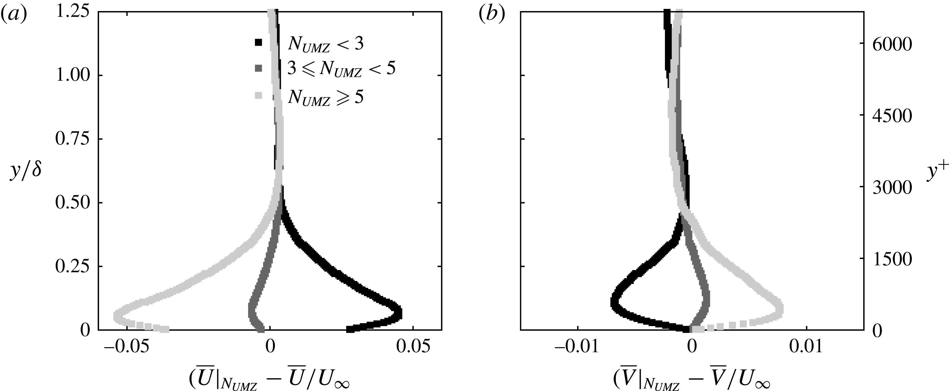
Apart from flow statistics, the time information available allows us to estimate time scales for the different events discussed above. In order to facilitate the discussion we define three characteristic groups:
 $N_{UMZ}<3$
, representing low number of zones;
 $3\leqslant N_{UMZ}<5$
average number of zones (
 $\overline{N}_{UMZ}\approx 3.2$
);
 $N_{UMZ}\geqslant 5$
large number of zones. The groups are defined in such a way that a low number of zones represents a large-scale
 $Q4$
event in the log region, while the high zone-number group represents a large-scale
 $Q2$
. Both velocity components are close to the global average for the average zone-number group (see figure 15
a,b).
Conditionally averaged velocities for each characteristic zone-number group. (a) Difference from global streamwise average. (b) Difference from global wall-normal average.

5.1 Number of zones
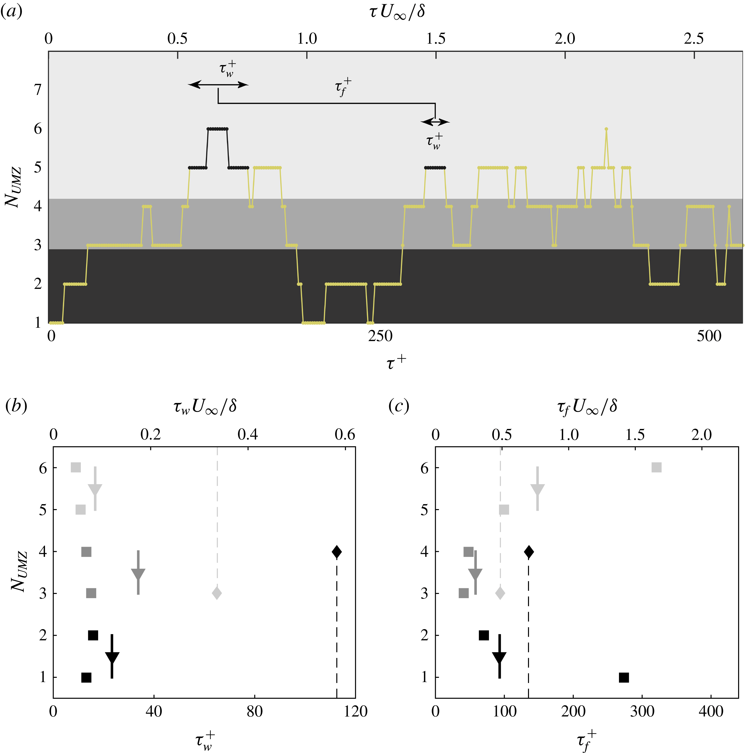
Since UMZs with short temporal coherence have been removed, we can estimate the time for which a certain zone-number structuring resides within our FOV, and how often this structuring reappears. This definition is shown schematically in figure 16(a) for an example of 300 consecutive images. The residence time of a certain number of zones or group of zones (the large number of zones group is highlighted here) inside the measurement plane is denoted with
 $\unicode[STIX]{x1D70F}_{w}^{+}$
, while
 $\unicode[STIX]{x1D70F}_{f}^{+}$
denotes the time after which the same
 $N_{UMZ}$
or group of zones reappears.
(a) Time evolution of
 $N_{UMZ}$
(time-coherent UMZs) for the same 300 consecutive images as in figure 4(c). Background colours denote the classification of
 $N_{UMZ}$
into the three groups defined in figure 15. Examples of how long a high number of zones resides within the measurement plane,
 $\unicode[STIX]{x1D70F}_{w}^{+}$
, and how often it reappears,
 $\unicode[STIX]{x1D70F}_{f}^{+}$
, denoted with black. (b,c) For how long, on average, the boundary layer is structured into a certain number of zones (b) and the frequency of repetition of this structuring (c). Each number of zones is marked with ◼ and each characteristic group with ▼. Solid lines mark the range of each group. Colours as in figure 15. ♦ Symbols denote the time (b) and frequency (c) for which the boundary layer is structured in an average or high number zones (light grey) or in a low or average number of zones (black), while dashed lines mark the range of each of these cases respectively.

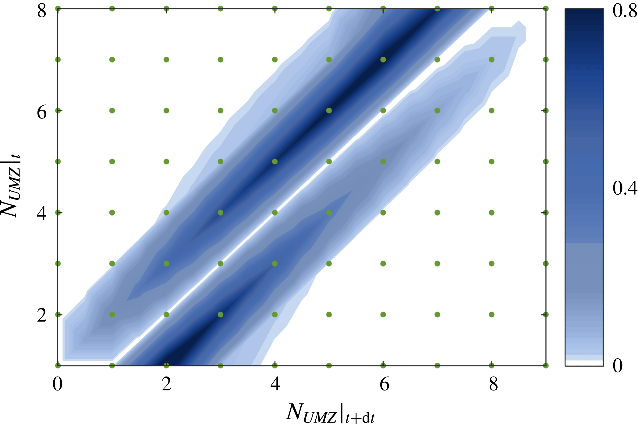
The PDF of the number of zones at time
 $t+\text{d}t$
, based on the number of zones at time
 $t$
. Green dots denote data points. Linear interpolation was used on a finer mesh for visual clarity.

The average residence time of the different zone-number states is found to be of the order of 10 viscous time units and exhibits only a very slight decreasing trend as
 $N_{UMZ}$
increases (figure 16
c). The frequency with which each number of zones appears in time reflects the PDF distribution of
 $N_{UMZ}$
(figure 5); increase in frequency is observed for an average number of zones, while both extremes appear progressively less often (figure 16
d). A change in the relative time scales is expectedly observed when instead of individual zones, the three characteristic zone-number groups are considered. The average zone-number group exhibits residence times almost twice as long as either of the high or low zone-number groups and it is also the most frequent state (as was expected from the PDF distribution of
 $N_{UMZ}$
). As can be seen in figure 16(a), the transition from the average state to either extreme is not monotonic. This implies that, starting at the most frequent state of an average
 $N_{UMZ}$
, there could be a shift towards an extreme (either high or low), a return to an average number of zones, and a shift again towards the same extreme. The time scales of all such transitions were reported above, however it was the presence of one extreme or the other that was shown in the previous section to be linked with large-scale structures in the log layer. Therefore, the residence time of a high or average zone-number state (
 ${\sim}0.33\unicode[STIX]{x1D6FF}/U_{\infty }$
) that does not get into a low zone behaviour (marked with

 ${\sim}0.58\unicode[STIX]{x1D6FF}/U_{\infty }$
) of a low or average number of zones, could indicate the presence of a high-speed structure that was previously shown to be linked with it.
Apart from the time scales, we can further investigate the evolution of this structuring process by finding the most probable number of UMZs at a time
 $t+\text{d}t$
, given that at time
 $t$
, the flow is organised into
 $N_{UMZ}$
. As was discussed, the time step
 $\text{d}t$
after which a change occurs, has a weak dependence on the number of zones at time
 $t$
and is of the order of 10 viscous time units. Results show that the division of an average number of zones (
 $3\leqslant N_{UMZ}<5$
) is the most preferable state (figure 17). Given a low
 $N_{UMZ}$
the most probable change will be towards a higher number, while given a high number of UMZs at time
 $t$
, the opposite trend is observed. For an average
 $N_{UMZ}$
, there is almost equal probability of moving towards either a lower or a higher number of zones. It is interesting to note that all zone-number changes are symmetric. For example a change from a structuring of
 $N_{UMZ}=5$
to one with
 $N_{UMZ}=3$
will happen approximately as many times as the reverse (
 $N_{UMZ}=3$
followed by
 $N_{UMZ}=5$
). Due to this symmetry, when estimating the most probable situation that preceded (at time
 $t-\text{d}t$
) each realisation at time
 $t$
, the results are almost identical to the ones presented in figure 17.
5.2 Individual UMZs
The analysis of the previous section was relevant to the time scales and evolution of the structuring process of the boundary layer into a given number of zones. However, the results did not include information on the temporal coherence of individual UMZs. Each zone is detected based on modal velocities that are present in each snapshot. Several of the detected peaks also appear in following snapshots, while others die away. Based on the change of each peak’s modal velocity in consecutive snapshots, individual UMZs can be tracked. As mentioned above, we only consider peaks that persist inside the FOV for times longer than
 $\unicode[STIX]{x1D70F}^{+}\approx 20$
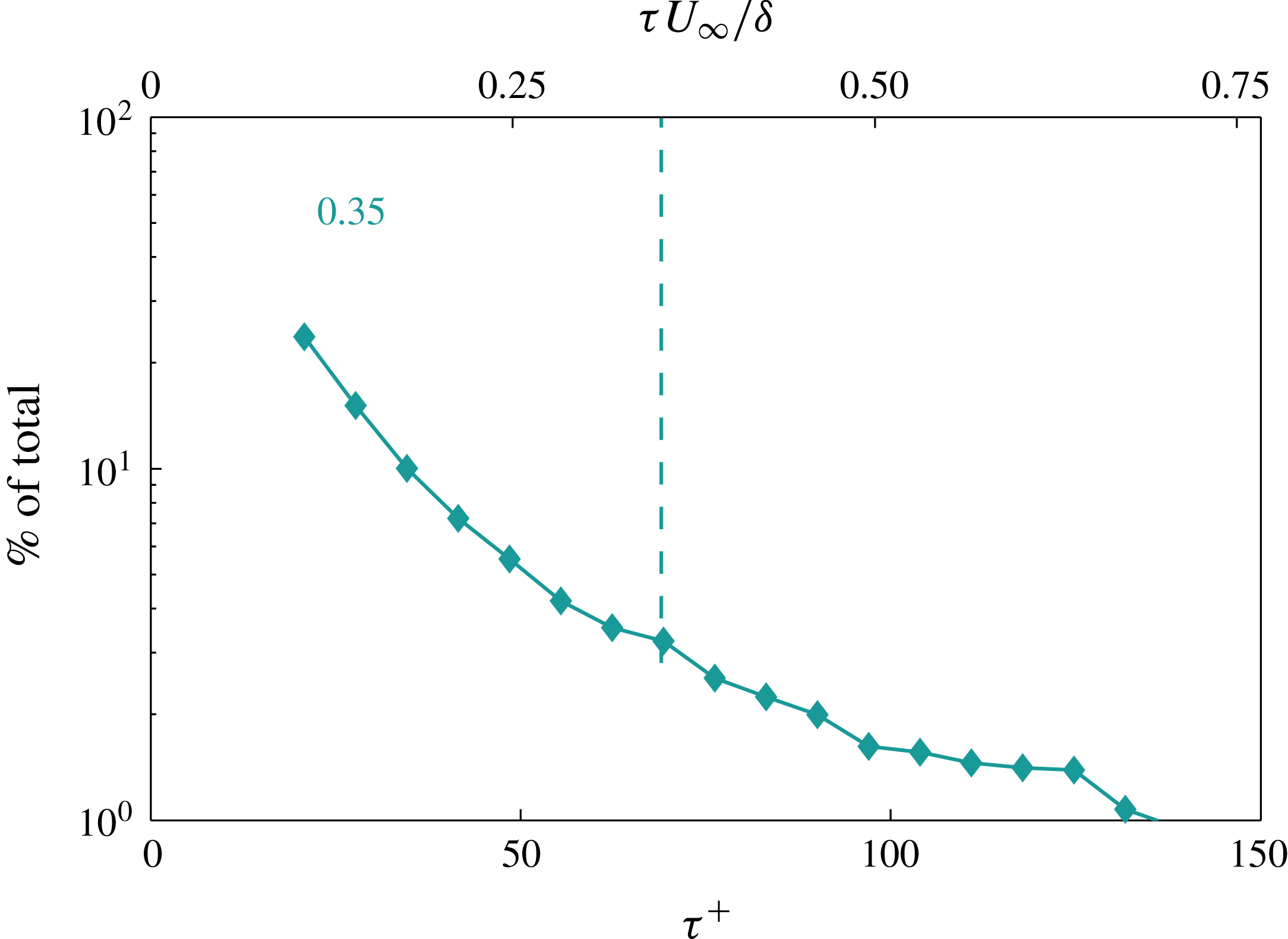
. For these peaks, the average residence time is
 ${\approx}0.35\unicode[STIX]{x1D6FF}/U_{\infty }$
and shows that these structures persist within our FOV for time scales shorter than
 $\unicode[STIX]{x1D6FF}/U_{\infty }$
(figure 18). As was mentioned in the previous section, UMZs are shown to be linked with large-scale structures in the log region, however their temporal coherence is based on the time that a single modal velocity persists within the measurement plane and as such are generally expected to have much shorter time scales than the corresponding log region events. The largest residence times found (
 $6-7\unicode[STIX]{x1D6FF}/U_{\infty }$
), show that there are cases where individual UMZs do indeed reach time scales that, assuming convection velocities that range from
 $0.5-0.9U_{\infty }$
, may indicate structures with lengths larger than
 $3\unicode[STIX]{x1D6FF}$
(LSMs) and reaching up to
 $6\unicode[STIX]{x1D6FF}$
(superstructures).
Frequency of appearance of time-coherent UMZs (in
 $\%$
of the total), depending on their residence time,
 $\unicode[STIX]{x1D70F}$
. Dashed line denotes average residence time.

Large-scale structures and superstructures are also known to meander in the spanwise direction and therefore it is likely for them to appear and disappear from our streamwise–wall-normal measurement plane, effectively breaking their observed time coherence and as such the residence times of UMZs as well, depending on their meandering amplitude and alignment with the FOV. Another explanation for the lack of longer residence times, comes from recent studies suggesting that the observed spectral peaks in the outer region that have been linked to the presence of very large structures, might be due to a sequence of structures that are repeated in time for very long distances, without necessarily an elongated spatial coherence: Kim & Adrian (Reference Kim and Adrian1999) and later Baltzer, Adrian & Wu (Reference Baltzer, Adrian and Wu2013) suggested that the large-scale motions (LSMs) observed in high
 $Re$
pipe flows align to form VLSMs, an observation later supported by Lee & Sung (Reference Lee and Sung2011) for superstructures in turbulent boundary layers. Following this reasoning, Hellström, Ganapathisubramani & Smits (Reference Hellström, Ganapathisubramani and Smits2015) and Ahn et al. (Reference Ahn, Lee, Lee, Kang and Sung2015) using experimental and numerical data of a pipe flow respectively, showed that the observed coherence of the very large structures in the frequency domain does not infer spatial coherence of the same size and that the emerging outer spectral peak reflects an alignment of smaller structures.
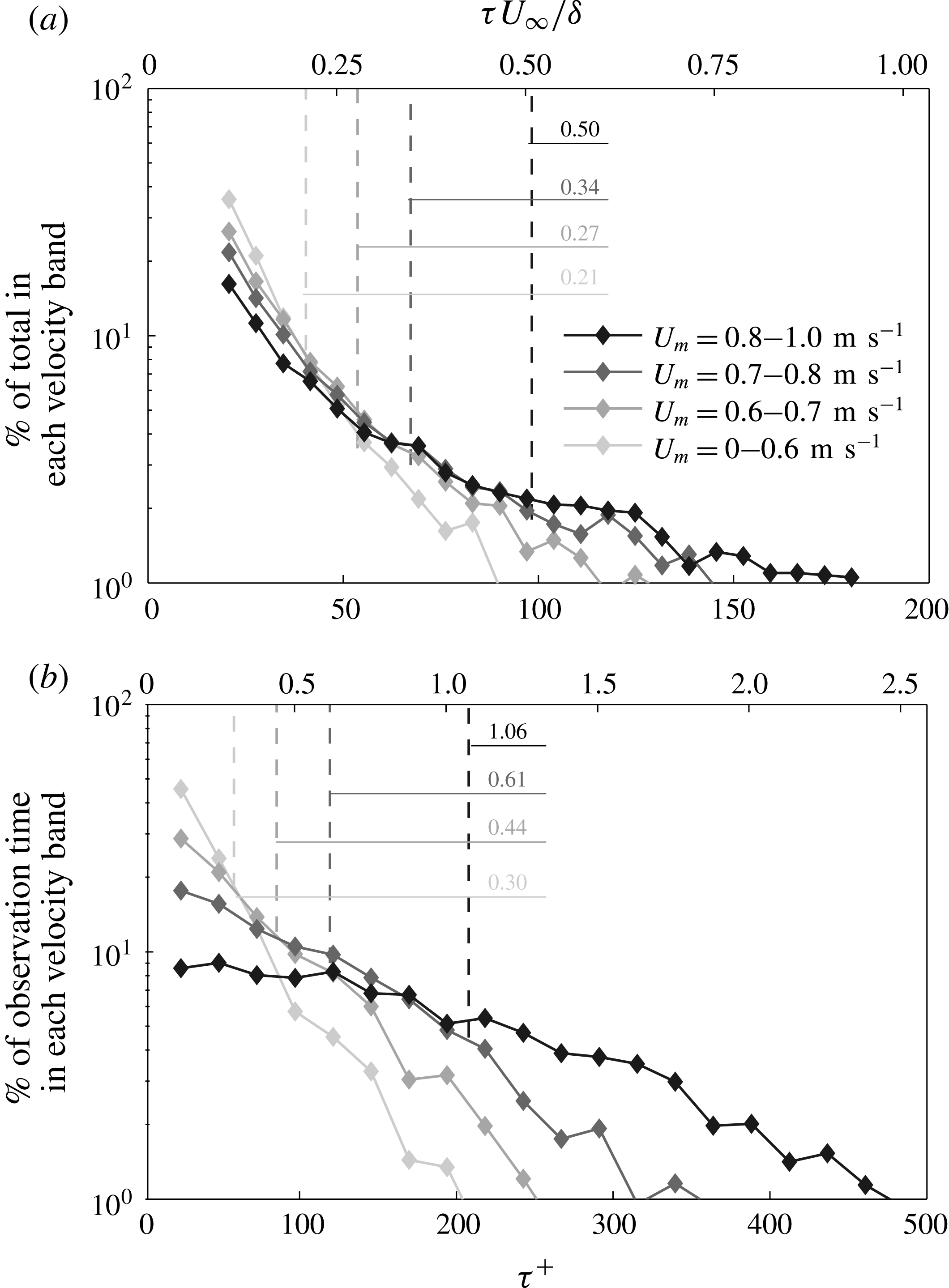
UMZs are classified according to whether they reach a modal velocity,
 $U_{m}$
belonging to each of the three shown velocity bands, at least once during their residence time
 $\unicode[STIX]{x1D70F}$
. (a) Frequency of appearance of UMZs within each velocity band (in
 $\%$
of the total UMZs within that band), depending on their residence time. Each UMZ might contribute to multiple bands, only once to each, according to the different modal velocities it corresponds to during its residence time. Dashed lines denote the average residence time of UMZs within each band. (b) Duration of observation of UMZs within each velocity band (in
 $\%$
of the total observation time of all UMZs within that band) according to their residence time. Each UMZ might contribute to multiple bands, every time it reaches a modal velocity belonging to any of them. Dashed lines denote the average observation time of UMZs in each group.

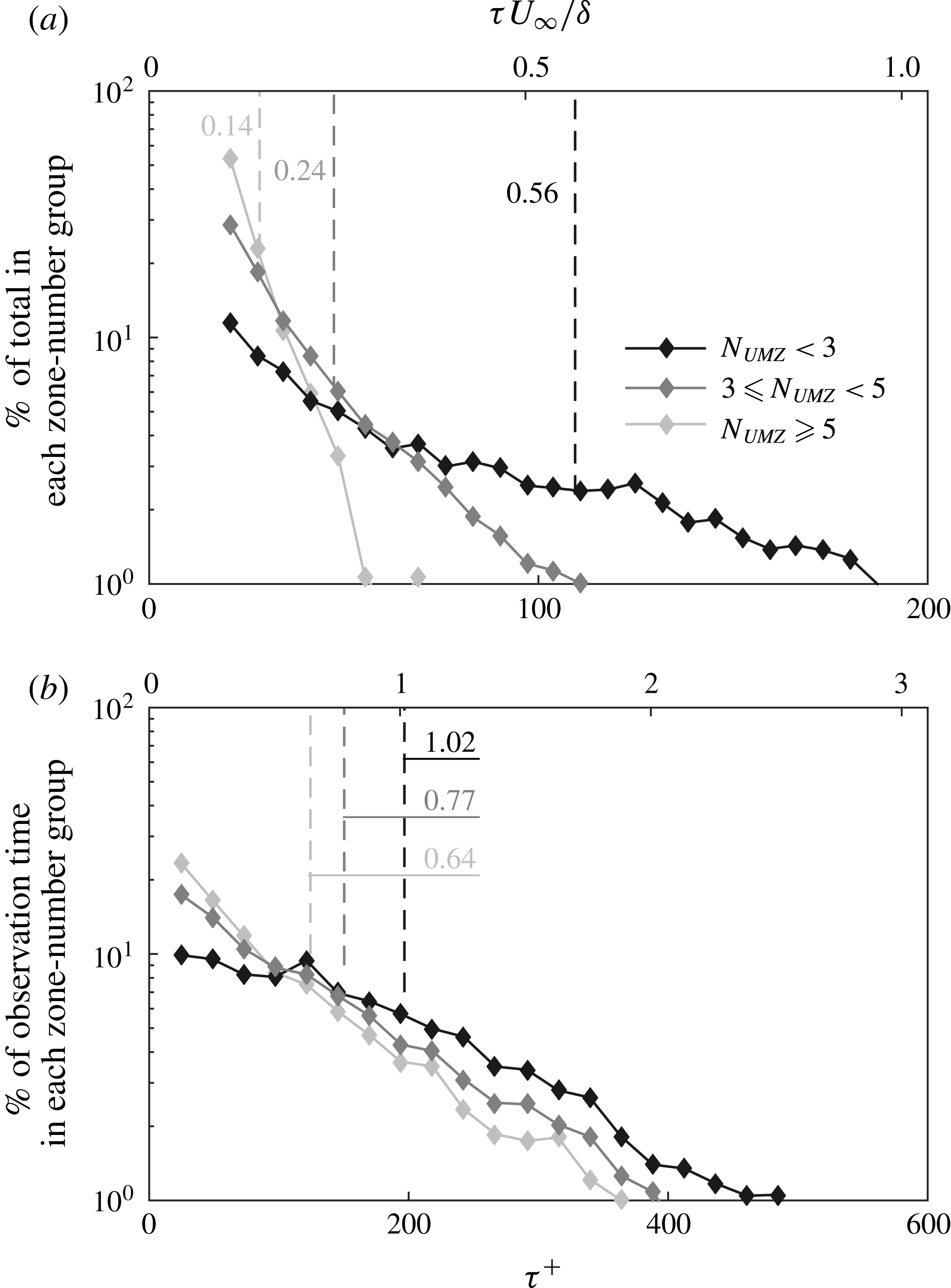
Throughout each zone’s residence time within the FOV, both their respective rank as well as the number of zones present at every snapshot vary. The naturally arising question is whether the modal velocity of each zone and the total number of zones present in the flow during each zone’s residence time have any influence on that characteristic time. The time sequence presented in figure 4(c) shows that zones with large modal velocities have larger time scales than the ones that appear closer to the wall. This is further supported from the residence time of structures that, during this time, have a modal velocity belonging to one of the four modal velocity groups shown in figure 19(a). Each zone might contribute to all groups (only once to each though), according to the different modal velocities it corresponds to during its residence time. Although each modal velocity band contains zones that persist within the measurement plane for various times, there is a clear increase of the average residence time (denoted with dashed lines), for zones closer to the free stream. Also, even though low modal velocity bands include some UMZs with long residence times, the majority of their observation time includes UMZs with shorter time scales (see figure 19
b). For example, 50 % of the total observation time of the lowest modal velocity group (denoted with light grey in figure 19) is spent on structures with residence times shorter than
 $\unicode[STIX]{x1D70F}^{+}=40$
. For the high modal velocity bands, the observation time is almost equally spent between structures of all time scales. This essentially means that for any individual snapshot, it is much more probable for a high modal velocity peak to have a long residence time than it is for a low modal velocity peak one. Furthermore, the mean observation times of each velocity group show that in any individual snapshot there is also a much higher probability of finding a peak that belongs in a high velocity group. That trend supports a hierarchical organisation of structures in the wall-normal direction (new slower zones appearing close to the wall, while older faster ones are located closer to the free stream) and is also in line with the schematic depiction of a hairpin packet organisation by Adrian et al. (Reference Adrian, Meinhart and Tomkins2000).
UMZs are classified according to whether they encounter any of the three shown zone-number groups, at least once during their residence time,
 $\unicode[STIX]{x1D70F}$
. (a) Frequency of appearance of UMZs, within each zone-number group (in
 $\%$
of the total within that group), depending on their residence time. Each UMZ might contribute to multiple groups, only once to each, according to the number of other zones appearing and dying away during its residence time. Dashed lines denote the average residence time of UMZs within each group. (b) Duration of observation of UMZs within each zone-number group (in
 $\%$
of the total observation time of all UMZs within that group) according to their residence time. Each UMZ might contribute to multiple groups, every time it encounters them. Dashed lines denote the average observation time of UMZs in each group.

When the residence times are grouped according to
 $N_{UMZ}$
the results show that zones appearing in snapshots where the boundary layer is organised into many layers are less coherent in time (mean residence times of
 $0.14\unicode[STIX]{x1D6FF}/U_{\infty }$
) and even the longer ones do not typically exceed residence times of
 $0.25\unicode[STIX]{x1D6FF}/U_{\infty }$
(figure 20
a). Also, in the high number of zones group, shorter-lived structures are shown to dominate the total time of peak observation (figure 20
b). This shows that for any snapshot belonging to a high zone-number group, there is a much higher possibility that any of the peaks present is a short-lived one. On the other hand, UMZs that exist in snapshots characterised by a low
 $N_{UMZ}$
, tend to persist much longer (on average almost 4 times longer than the high zone-number group), with maximum residence times exceeding
 $\unicode[STIX]{x1D6FF}/U_{\infty }$
and they are also shown to spend the majority of these residence times in the low zone-number group (figure 20
b). For example, zones with residence times of
 $\unicode[STIX]{x1D70F}^{+}=250$
account for 4.5 % of the total observation time of the low zone-number group, while only for 1 % of the total observation time of the high zone-number group. This trend can be mapped into a Reynolds number dependency following the scaling of the number of zones with
 $Re_{\unicode[STIX]{x1D70F}}$
(de Silva et al.
Reference de Silva, Hutchins and Marusic2016). More specifically, a low number of zones (
 $N_{UMZ}<3$
) would correspond to a
 $Re_{\unicode[STIX]{x1D70F}}\sim 10^{3}$
while a high number of zones to a
 $Re_{\unicode[STIX]{x1D70F}}\sim 10^{4}$
suggesting that the UMZs present in the flow tend to decrease in size and extent as the Reynolds number increases. A similar behaviour was reported by Vallikivi, Ganapathisubramani & Smits (Reference Vallikivi, Ganapathisubramani and Smits2015), who found that the wavelength of the outer spectral peak increases when normalised with inner variables and decreases in the case of an outer-scale normalisation, suggesting that the scales associated with it decrease in size as the Reynolds number increases. Another explanation for this time scale variation could come from the organisation of the flow in the log region. More specifically, it was shown above that a low number of zones is on average correlated with a large-scale
 $Q4$
event in the log layer, while a
 $Q2$
most often leads to a high number of zones. Lozano-Duran et al. (Reference Lozano-Duran, Flores and Jimenez2012) showed that, large-scale
 $Q4$
events exist in pairs with
 $Q2$
structures and that low-speed events are often engulfed by high-speed ones and are significantly smaller in length and width. This documented difference in size, could be the reason for the much larger time scales observed when the number of zones is low.
6 Summary and discussion
The previous findings can be summarised in a conceptual model of the flow (figure 21), that combines the conditional velocity profiles, with the resulting number of UMZs in the flow and their time scales. Two extreme cases are presented, namely the flow organisation into a high (light grey) and low (dark colours) number of zones. As was discussed in previous sections, the former corresponds to a large-scale ejecting motion in the logarithmic layer. The turbulent activity within the log region in that case is significantly higher, due to the presence of a large-scale low momentum event. A flow organisation into a low number of zone is linked on the other hand with a high-speed event in the log region, which is responsible (according to amplitude modulation concepts) for a decrease in turbulent activity within that region.
Conceptual model summarising the results. Large-scale events in the outer layers together with the corresponding flow statistics (see also figure 11) and the most probable resulting number of zones. Light grey colour represents a large-scale
 $Q2$
event and a corresponding high number of zones, while black denotes a low number of zones linked with a large-scale
 $Q4$
event in the log region. Representative examples of snapshots with a high and low number of zones are also depicted. The TNTI location in both snapshots is marked with solid black line.

Several studies have shown that these log-layer structures exist in side-by-side pairs that meander in the spanwise direction (Hutchins & Marusic Reference Hutchins and Marusic2007b ; Dennis & Nickels Reference Dennis and Nickels2011; Lee & Sung Reference Lee and Sung2011; Lozano-Duran et al. Reference Lozano-Duran, Flores and Jimenez2012; Zheng & Longmire Reference Zheng and Longmire2014, among others). Using a similar conceptual model, we can represent the two very distinct flow states discussed above, with different spanwise locations within this coalition of structures (solid light grey and black lines in figure 21).
7 Conclusions
The structuring of a turbulent boundary layer into uniform momentum zones was analysed using time-resolved planar PIV. The main geometrical characteristics and time evolution of the zones were presented and it was shown that the total number of zones in the flow is linked with different large-scale events in the log layer. More specifically, a high number of zones is usually linked with a large-scale
 $Q2$
event. The low-speed fluid moving upwards creates increased small-scale activity above the cross-over point, in line with previous amplitude modulation findings. Conversely, a low number of uniform momentum zones corresponds to a large-scale
 $Q4$
event in the log region and decreased turbulent activity away from the wall. Earlier studies have reported the existence of alternating large high- and low-speed structures in the log region that meander in the spanwise direction (Hutchins & Marusic Reference Hutchins and Marusic2007a
; Dennis & Nickels Reference Dennis and Nickels2011; Jiménez Reference Jiménez2013, among others). Based on these observations, the organisation of the boundary layer into a low or high number of zones can be considered the result of a high- or low-momentum structure moving through the measurement plane respectively.
In terms of temporal evolution, it was shown that the presence of a given number of zones is a viscous-scaled phenomenon in time. Time scales of individual UMZs (tracked in time based on their modal velocities), indicate that there is a scaling of the residence times of UMZs with wall-normal location as suggested by Adrian et al. (Reference Adrian, Meinhart and Tomkins2000), with older, larger zones being located closer to the free stream and moving faster. Furthermore, the events with the longest residence times belonged in their majority to a low zone-number structuring, while the zones present in high zone-number cases, exhibited shorter time scales. This behaviour reflects a decrease of temporal coherence for conditions that simulate a higher Reynolds number flow. Finally, for all detected UMZs (and assuming an appropriate convection velocity), the corresponding spatial extents were shown to be much shorter than the large-scale structures found in boundary layers, thus indicating either very long structures meandering in the spanwise direction or a streamwise alignment of much shorter events. Based on these observations, future research could be directed at datasets of much longer streamwise extent in order to facilitate such a distinction. Also, similar analysis of time-resolved spanwise – wall-normal velocity snapshots could elucidate the spanwise behaviour and extent of UMZs and potentially provide a physical description of what could only be a conceptual interpretation here.
Acknowledgements
The authors acknowledge the financial support of the European Research Council (ERC grant agreement no. 277472), and the Engineering and Physical Sciences Research Council of the United Kingdom (EPSRC grant ref. no. EP/L006383/1 and RCUK Doctoral training grant no. 1360741). R.d.K. is partially supported by a Leverhulme Early Career Fellowship and R.J.H. is partially funded by NSERC (Natural Sciences and Engineering Research Council of Canada). A.L. is supported by the Zonta International Foundation (Amelia Earhart fellowship). The experimental dataset used in this study is openly available from the University of Southampton repository at: https://doi.org/10.5258/SOTON/D0160.
Supplementary movies
Supplementary movies are available at https://doi.org/10.1017/jfm.2018.126.
Appendix A. Turbulent/non-turbulent interface detection
The detection of the TNTI has been, in itself, the focus of a variety of studies over the years and many different methods have been developed, mainly corresponding to the experimental or numerical method used to acquire the data. While details on the subject are out of the scope of this work, a brief outline on the chosen detection method follows for completeness.
Since only velocity information is available in a two-dimensional domain and based on the limitations of using a vorticity threshold on a noisy free stream, we chose to use a kinetic energy deficit threshold, as described in Chauhan et al. (Reference Chauhan, Philip and Marusic2014a
,Reference Chauhan, Philip, de Silva, Hutchins and Marusic
b
). A local instantaneous kinetic energy deficit,
 $K$
, over a
 $3\times 3$
region, on a coordinate system moving with the free stream velocity,
 $U_{\infty }$
, is given by:
 $$\begin{eqnarray}K=100\times \frac{1}{9U_{\infty }^{2}}\mathop{\sum }_{m,n=-1}^{1}[(U_{m,n}-U_{\infty })^{2}+V_{m,n}^{2}].\end{eqnarray}$$
Above the TNTI, i.e. at the free stream,
 $U\approx U_{\infty }$
and
 $V\approx 0$
, therefore
 $K$
is expected to be very small, whereas below the interface and towards the wall, where the turbulent fluctuations are more energetic, the value of
 $K$
rapidly increases. A threshold,
 $K_{th}$
can then be computed, using the average turbulent kinetic energy in the free stream from all the available velocity snapshots, above which the flow is considered turbulent. For the present data, the average kinetic energy deficit computed in the free stream was 0.16. Based on this threshold, a binary representation of the flow is computed for which, regions with a local
 $K$
below the threshold are assumed to be non-turbulent (and are assigned a value of 1), while regions with
 $K>K_{th}$
are considered turbulent (and are assigned a value of 0). Then the interface location is estimated as the shortest continuous contour line with a value of 0.5. However, the ultimate choice of a momentum deficit threshold (starting from the average value in the free stream), is subject to a number of considerations, in order for the TNTI definition to be consistent with the boundary layer thickness (Chauhan et al.
Reference Chauhan, Philip, de Silva, Hutchins and Marusic2014b
). In the present work, because of higher turbulence intensity levels in the free stream – mostly due to the different medium used (water) – a higher threshold is required, chosen such that the average TNTI statistics were comparable with those from Chauhan et al. (Reference Chauhan, Philip, de Silva, Hutchins and Marusic2014b
), while also taking into account the proposed considerations. More specifically, based on the variation of both the intermittency profiles as well as the TNTI statistics with
 $K_{th}$
, a threshold of
 $K_{th}=0.26$
was chosen, such that the resulting intermittency profile (marked with red in figure 22
a) was approximately constant above
 $\unicode[STIX]{x1D6FF}$
, while also
 $\overline{Y}_{i}+3\unicode[STIX]{x1D70E}_{i}<1.4\unicode[STIX]{x1D6FF}$
, and
 $\overline{Y}_{i}\approx 0.6\unicode[STIX]{x1D6FF}$
. Using this threshold, the PDF of the vertical TNTI location showed a positive skewness towards the wall (figure 23) a behaviour attributed to the aforementioned increased turbulence intensity. The mean location of the TNTI was found to be at
 $\overline{Y}_{i}=0.58\unicode[STIX]{x1D6FF}$
. Lower values of
 $K_{th}$
were also tested and while the above statistics varied (see figure 22
a,b), the final choice of the threshold was found to be inconsequential to the results presented in the main sections of this work.
(a) Variation of the intermittency profile with
 $K_{th}$
. Fully turbulent flow at
 $\unicode[STIX]{x1D6FE}=0$
, while no turbulent activity is considered at the limit of
 $\unicode[STIX]{x1D6FE}=1$
. Solid red line marks the chosen threshold
 $K_{th}=0.26$
and dashed red line denotes the boundary layer thickness above which the kinetic energy deficit profile should be approximately constant. (b)
 $\overline{Y}_{i}+3\unicode[STIX]{x1D70E}_{i}$
. Solid red circle denotes the chosen threshold
 $K_{th}=0.26$
.

The PDF of TNTI location,
 $Y_{i}$
. Dashed line denotes the corresponding Gaussian distribution with
 $\unicode[STIX]{x1D707}=\overline{Y}_{i}$
,
 $\unicode[STIX]{x1D70E}=\unicode[STIX]{x1D70E}_{i}$
. Dotted-dashed line denotes
 $\overline{Y}_{i}=0.58\unicode[STIX]{x1D6FF}$
.

Finally, it should be noted here that, the process described above did not always result in a continuous contour covering the streamwise extent of the FOV in its entirety. Since these cases counted for a relatively small percentage (
 $5\,\%$
) of the total number of images (which included more than
 $405\,000$
snapshots), these instances were not included in any of the presented results.
Appendix B. Number of modal peaks detected – influence of bin count and time coherence
Apart from the parameters discussed in § 3 that have an influence on
 $N_{UMZ}$
, the temporal coherence of UMZs within the measurement plane is another important factor that should be considered. As was already mentioned, for all the results presented in this study, UMZs that have a temporal coherence shorter than
 $\unicode[STIX]{x1D70F}^{+}\approx 20$
are removed. This leads to an expected decrease in the average number of peaks detected (see figure 5), and also to some notable differences in the conditional averages presented in figures 10 and 11. More specifically, for an instantaneous peak detection, the average TNTI location,
 $\overline{Y}_{i}$
, shows a strong variation with the number of zones,
 $N_{UMZ}$
(figure 24
a). Interestingly, a low
 $\overline{Y}_{i}$
leads to a large
 $N_{UMZ}$
and vice versa. This can also be seen in the conditionally averaged profiles of
 $U$
and
 $V$
which, in the outer region exhibit a
 $Q2$
-like behaviour for a low
 $N_{UMZ}$
, while a
 $Q4$
motion is observed for a high
 $N_{UMZ}$
.
Flow statistics variation with
 $N_{UMZ}$
before removal of short-lived peaks. Colour gradient from dark to light denotes increasing number of zones. (a) Variation of the mean location of the TNTI,
 $\overline{Y}_{i}$
. Red dotted line denotes the global average location of the TNTI. (b,c) Difference of conditionally averaged streamwise and wall-normal velocity profiles from their respective global averages.

The PDF of
 $U/U_{\infty }$
for two independent velocity snapshots, representing a lower and a higher than average TNTI location and how that influences the detection of modal peaks. Red and green triangles denote peaks with streamwise extent below and above the defined threshold respectively. White lines mark the local minimum between two consecutive peaks. (a)
 $\overline{Y}_{i}=0.46\unicode[STIX]{x1D6FF}$
. (b)
 $\overline{Y}_{i}=0.98\unicode[STIX]{x1D6FF}$
.

This variation could be traced back to the physical description of the zones. UMZs are defined as local peaks of the streamwise velocity PDF. If the free stream velocity is considered relatively constant within all available snapshots, a low TNTI leads to a very fast transition of low velocities near the wall to free stream values at the edge of the boundary layer. In such cases, a much smaller amount of vectors of the same velocity band can form a detectable UMZ, thus enabling the formation of multiple zones, smaller in size, that are also expected to have smaller time scales. The use of a temporal threshold to remove short-lived peaks, would therefore act as a balance for the large increase in
 $N_{UMZ}$
observed for low TNTI locations. Additionally, a higher than average TNTI location, is in many cases a result of snapshots with elevated free stream turbulence intensity, the presence of which might interrupt the time coherence of the peaks detected below it. Removal of short-lived peaks will therefore tend to balance the TNTI variation further, leading to an almost constant TNTI location for all
 $N_{UMZ}$
(figure 10).
Based on these observations, it is important to check whether this variation potentially stems from a bias of the instantaneous detection procedure, due to the decrease in bin counts and increase of detection noise in the case of low
 $\overline{Y}_{i}$
.
The detection of a local peak is based on its prominence with respect to the neighbouring points. For each peak, this can be represented as the difference in bin counts, between the peak itself, and the neighbouring local minimum
 $\unicode[STIX]{x0394}N=N_{peak}-N_{min}$
. Since the number of vectors in each bin,
 $N$
, is a result of a counting procedure, it is associated with a Poisson distribution and therefore its uncertainty estimate is the standard deviation of the Poisson distribution for the counted value,
 $\sqrt{N}$
. Following a linear propagation analysis (JCGM 2008), the corresponding uncertainty on the difference of bin counts can then be estimated as
 $\sqrt{N_{peak}+N_{min}}$
. So, the certainty with which a peak is detected depends on whether its prominence from the neighbouring bins is greater than the uncertainty involved in its detection. It should be noted here that, since each peak is bounded by two local minima, the greater of the two is chosen in order to account for the worst-case scenario.
A typical example of a low TNTI (figure 25(a),
 $\overline{Y}_{i}=0.46\unicode[STIX]{x1D6FF}$
), shows that in total, seven peaks are detected instantaneously, of which only the first three (marked with green triangles) are time coherent. On the other hand, a higher than average TNTI location (figure 25(a),
 $\overline{Y}_{i}=0.98\unicode[STIX]{x1D6FF}$
) leads to the detection of three peaks that are all time coherent.
Difference in vector counts,
 $\unicode[STIX]{x0394}N=N_{peak}-N_{min}$
, between the modal peaks in figure 25 and the greater of the two local minima that surround them. Grey lines mark the uncertainty on the detection of each peak, defined as
 $\sqrt{N_{peak}+N_{min}}$
. (a)
 $\overline{Y}_{i}=0.46\unicode[STIX]{x1D6FF}$
. (b)
 $\overline{Y}_{i}=0.98\unicode[STIX]{x1D6FF}$
.

As expected, when the TNTI is low, there is a significant decrease in the bin count, especially for the peaks that are short lived (red triangles in figure 26 a), for which the corresponding uncertainty is comparable although still lower than the prominence of the peaks. For the time-coherent peaks, although the uncertainty is increased, it is still an order of magnitude less than the peak prominence, ensuring that these peaks are well defined. On the other hand, when the TNTI is far away from the wall, the number of vectors for each detected peak is much larger (an order of magnitude larger for the peaks closest to the free stream), and the corresponding uncertainty is statistically insignificant for the detection of the peaks (figure 26 b).
The previous two cases show that instantaneously, a peak-detection algorithm will distinguish local maxima in the streamwise velocity PDF, based on the relative parameters discussed in § 3. However, the number of vector counts for each peak with respect to its neighbouring minimum is another crucial parameter that influences the confidence bound with which each peak is detected. In cases where the TNTI is located very close to the wall and only a small number of velocity vectors are available below it, more peaks are detected on average but with much higher uncertainty levels. Therefore, care should be taken especially for the short-lived modal peaks, since in some cases their prominence with respect to neighbouring points is of the order of their detection uncertainty. Interestingly, time coherence of the peaks seems to ensure a prominence much greater than the relevant uncertainty, even in cases where the TNTI is very close to the wall.