1. Introduction
A point vortex transforms into a hollow vortex when the pressure at its core falls below the vapour pressure of the surrounding liquid. This phenomenon is observed in various natural and industrial applications, such as tornadoes, tip vortex cavitation on marine propellers, vortex rope cavitation in the draft tubes of Francis turbines, and the formation of hollow vortices in high-speed industrial mixers and separators. The interior of a hollow vortex typically contains vapour or air, with a density much lower than that of the surrounding liquid. As a result, the interaction between the core contents and the liquid boundary is negligible, allowing the pressure within the hollow region to be treated as constant. Outside the core, the flow is assumed to be incompressible and irrotational.
Theoretical investigations of hollow vortices date back over a century to the foundational works of Hicks (Reference Hicks1883) and Pocklington (Reference Pocklington1895). Since then, more advanced and generalised models have been developed that account for non-trivial core dynamics, complex boundary conditions, and external influences, including background vorticity (Saffman Reference Saffman1992).
In recent years, the hollow vortex model has received much attention, and a number of analytical solutions have been developed to describe hollow vortices in various configurations. Notable contributions include the work of Baker, Saffman & Sheffield (Reference Baker, Saffman and Sheffield1976), who obtained exact steady solutions for a linear array of hollow vortices. Lin & Landweber (Reference Lin and Landweber1977) constructed a one-parameter family of exact solutions corresponding to Lavrentiev’s bubble separation model around a blunt two-dimensional body. Telib & Zannetti (Reference Telib and Zannetti2011) presented an analytical solution for steady inviscid separated flows, modelling the separation region as a hollow vortex. Llewellyn Smith & Crowdy (Reference Llewellyn Smith and Crowdy2012) analysed both the shape and stability of an isolated, steady hollow vortex subjected to a straining field. Zannetti & Lasagna (Reference Zannetti and Lasagna2013) investigated the Pocklington hollow vortex, replacing stagnation points with a Chaplygin cusp body. More recently, Green (Reference Green2015) studied a co-travelling hollow vortex pair and a single row of hollow vortices in a channel, extending several classical configurations. Christopher & Llewellyn Smith (Reference Christopher and Llewellyn Smith2021) – hereafter CLS2021 – examined the equilibrium shapes of vortices in corner geometries, further enriching the theory of hollow vortex structures.
All of the studies mentioned above do not account for surface tension in the formulation of the problem. Surface tension introduces additional complexity because the velocity magnitude along the free surface is no longer constant, due to the pressure jump that depends on the local curvature of the interface. Most studies that account for surface tension are related to waves on free surfaces or at the interface between two immiscible liquids (see Christodoulides & Dias Reference Christodoulides and Dias1994; Dias & Iooss Reference Dias and Iooss1996). Dias & Kharif (Reference Dias and Kharif1999) provided a comprehensive review, emphasising the bifurcation, stability and evolution of capillary–gravity waves, covering both steady and unsteady free-surface flows, including solitary waves, periodic waves and jet flows.
The number of studies on hollow vortices with surface tension is relatively small. Early work by Joukowski (Reference Joukowski1891) incorporated surface tension into Bernoulli’s equation, yielding fully nonlinear solutions in terms of rational functions for flows such as a bubble between two parallel plates. Subsequent efforts extended this approach to flows past cylindrical shells and bubbles, as shown by McLeod (Reference McLeod1955). Crapper (Reference Crapper1957) developed an exact solution for capillary wave trains in irrotational flows of infinite depth. This was later generalised to finite depth by Kinnersley (Reference Kinnersley1976).
Notable additional contributions include the work of Shankar (Reference Shankar1992), who studied a non-rotating hollow vortex with surface tension in a uniform stream. He applied a conformal mapping from the exterior of the unit circle in the auxiliary
 $\zeta \hbox{-}$
plane to the exterior of the bubble in the physical
 $z\hbox{-}$
plane, expressed in the form of a Laurent series. The unknown coefficients were determined by enforcing the Bernoulli equation on the bubble surface. This led to an infinite nonlinear system of equations that, in general, must be solved numerically. Shankar then proposed analytical asymptotic solutions by assuming an elliptical bubble shape. Shapes with
 $m\hbox{-}$
fold symmetry for
 $m\gt 2$
were not investigated.
Crowdy (Reference Crowdy1999) analysed a related problem of a non-rotating hollow vortex with twofold symmetry in an unbounded flow domain. To solve it, he introduced a method based on reformulating the Bernoulli condition as analyticity requirements on the conformal map, the complex potential, and a composite function constructed from them (Crowdy Reference Crowdy2000). Wegmann & Crowdy (Reference Wegmann and Crowdy2000) extended the exact twofold symmetry solutions of Crowdy (Reference Crowdy1999) to the case of general
 $m\hbox{-}$
fold symmetry. They obtained an infinite discrete set of circulation values at which
 $m\hbox{-}$
fold symmetric solutions exist. The core of their method is the reformulation of the bubble-shape problem as a conformal mapping problem combined with a functional equation for the mapping derivative, balancing hydrodynamic pressure and surface tension. They obtained closed-form solutions of this functional equation using rational functions, which yield rippled bubble shapes. The solution contains a continuous parameter that governs the shape of the bubble and plays the role of surface tension.
To the best of the authors’ knowledge, no equilibrium solutions for hollow vortices with surface tension are known in flow domains containing solid boundaries. Motivated by this gap, the present study investigates the boundary-value problem for a hollow vortex with surface tension in a corner geometry.
We apply the integral hodograph method to derive the complex velocity potential of the flow, satisfying fully nonlinear boundary conditions on both the free surface and the solid boundary of the corner. The velocity magnitude along the free surface is included in explicit form. We seek a hollow vortex that is symmetric about the corner bisector. This gives us the possibility to reduce the formulation of the problem from a doubly connected domain to a simply connected region in half of the flow domain. By imposing the dynamic boundary condition, we derive a singular integral equation for the velocity magnitude along the free surface, which is reduced to a system of nonlinear equations and solved using a collocation method. The results demonstrate how surface tension induces wave quantisation along the free surface, revealing equilibrium configurations not previously reported.
The problem is formulated in § 2, where the governing equations are derived. The parametric study of the vortex shape is presented in § 3.
2. Formulation of the problem
A sketch of the physical domain is shown in figure 1(a). We consider half of the flow domain inside a corner with interior half-angle
 $\alpha$
, bounded by a solid wall
 $AC$
along the positive
 $x$
-axis and the line of symmetry
 $AC^{\prime}$
. We have
 $0 \lt \alpha \lt \pi$
; in the special case
 $\alpha = \pi /2$
, the corner transforms into the upper half-plane bounded by a straight wall. The straight wall may be replaced by a symmetric hollow vortex in the lower half-plane, in which case the resulting flow without surface tension corresponds to the Pocklington dipole. The flow in a corner has no intrinsic length scale; therefore, we introduce a reference length
 $D$
, defined as the distance between the corner apex (point
 $A$
) and the centroid of the hollow vortex (point
 $Z_D$
), as shown in figure 1(a), or
 $D=|Z_D|$
. The coordinates of the centroid
 $Z_D$
and the area of the cavity are determined as
 \begin{equation} Z_D=\frac {1}{2A{\rm i}} \oint _C Z^2\, {\rm d}\overline{z}, \quad \overline{A}=\frac {1}{2{\rm i}}\oint _{\overline{C}} \overline {Z}\,{\rm d}Z, \end{equation}
where the contour
 $\overline {C}$
is taken around the whole flow region.
(a) The physical plane and (b) the parameter or
 $ \zeta$
-plane. Owing to the symmetry of the flow about the bisector line, only half of the flow domain is considered.

The complex potential for the flow around a corner without a vortex is given by
 $w = C_1 z^{(\pi /2\alpha)}$
, and the corresponding complex velocity is
 $ {\rm d}w/{\rm d}z = (\pi /2\alpha) C_1 z^{(\pi /2\alpha)-1}$
, where
 $C_1$
is a constant. It is evident that for
 $\alpha \neq \pi /2$
, there is no characteristic velocity: the velocity at infinity,
 $|z| \to \infty$
, tends to zero for
 $\pi /2 \lt \alpha \lt \pi$
, and it tends to infinity for
 $0 \lt \alpha \lt \pi /2$
. For the case
 $\alpha = \pi /2$
, the velocity at infinity is finite. If a point vortex of circulation
 $\varGamma$
is introduced at distance
 $D$
from the plane, then the velocity at infinity required to bring this vortex to rest, and so to induce a steady state, is
 \begin{equation} U = -\frac {\varGamma }{4\pi D}. \end{equation}
A hollow vortex is a steady, constant-pressure, two-dimensional region within an inviscid, incompressible and irrotational flow. Applying Bernoulli’s equation on the vortex boundary and incorporating the Young–Laplace relation for the pressure jump
 $p-p_c=\tau K$
, yields
 \begin{equation} V^2 + \frac {2\tau K}{\rho } = V_O^2 + \frac {2\tau K_O}{\rho }, \end{equation}
which relates the velocity magnitude and curvature between an arbitrary point on the boundary and a chosen reference point
 $O$
. Here,
 $V$
and
 $K$
denote the local velocity magnitude and the signed curvature of the boundary, respectively, while
 $V_O$
and and
 $K_O$
are their corresponding values at
 $O$
. The parameters
 $\tau$
,
 $\rho$
and
 $p_c$
denote the surface tension coefficient, the fluid density, and the pressure inside the vortex, respectively.
By expressing the velocity
 $V_O$
in terms of the circulation using
 $\varGamma =V_O D \gamma _D$
, the non-dimensional Bernoulli equation takes the form
 \begin{equation} v^2 + \frac {2 \kappa \gamma _D^2 }{{\textit{We}}_{\varGamma }} = 1 + \frac {2 \kappa _O\gamma _D^2 }{{\textit{We}}_{\varGamma }}, \end{equation}
where
 $v=V/V_O$
,
 $\kappa = KD$
,
 $\gamma _D$
is non-dimensional circulation, and
 $\textit{We}_{\varGamma }$
is the Weber number based on the circulation
 $\varGamma$
and the reference length
 $D$
:
 \begin{equation} {\textit{We}}_{\varGamma } = \frac {\rho \varGamma ^2}{\tau D}. \end{equation}
Alternative reference parameters could be the velocity magnitude at point
 $O$
and one of the lengths, the length
 $D$
or the length
 $L$
that is the distance between the corner point
 $A$
and the stagnation point
 $B$
(see figure 1). Then (2.4) takes the form
 \begin{equation} v^2 + \frac {2 \kappa }{{\textit{We}}} = 1 + \frac {2 \kappa _O}{{\textit{We}}}, \end{equation}
where
 $\textit{We} \in \{ {\textit{We}}_D, {\textit{We}}_L \}$
depending on the chosen reference length:
 \begin{equation} {\textit{We}}_D=\frac {\rho V_O^2 D}{\tau }, \quad {\textit{We}}_L=\frac {\rho V_O^2 L}{\tau }. \end{equation}
The relations between the Weber numbers are
 \begin{equation} {\textit{We}}_\varGamma ={\textit{We}}_D\, \gamma _D^2 = {\textit{We}}_L\, \gamma _L^2 \frac {L}{D}, \end{equation}
where
 $\gamma _L$
is non-dimensional circulation based on the reference length
 $L$
.
For
 $\alpha = \pi /2$
, the velocity at infinity
 $U$
is finite, and it is related to the velocity at point
 $O$
through the Bernoulli integral. Introducing the cavitation number
 \begin{equation} \sigma =\frac {2(p_\infty -p_c)}{\rho U^2}, \end{equation}
where
 $p_\infty$
and
 $p_c$
are the pressures at infinity and in the cavity, respectively, we obtain
 \begin{equation} U/V_O=v_\infty =\sqrt {\frac {1+2\kappa _O/{\textit{We}}}{1+\sigma }}. \end{equation}
2.1. Complex potential of the flow with a hollow vortex
The solution for the hollow vortex problem is obtained using the integral hodograph method, which is based on constructing expressions for the complex velocity and the derivative of the complex potential, both defined in an auxiliary parameter plane. In this formulation, the first quadrant of the parameter plane is chosen, where the imaginary axis corresponds to the free surface of the vortex, and the real axis represents the solid wall
 $AC$
and the intervals of the line of symmetry
 $OA$
and
 $C^\prime E$
, forming the closed contour
 $OABCC^\prime E$
.
According to the conformal mapping theorem, one has the freedom to specify the images of three boundary points arbitrarily in the parameter plane. These are:
 $O$
(
 $\zeta = 0$
),
 $CC^\prime$
(
 $\zeta = 1$
) and
 $E$
(
 $\zeta = \infty$
), as shown in figure 1(b). The positions of points
 $A$
(
 $\zeta = a$
) and
 $B$
(
 $\zeta = b$
) will be determined later based on physical considerations.
Let us assume that the magnitude of the velocity,
 $v(\eta) = \left | {\rm d}w/{\rm d}z \right |$
, is known as a function of the coordinate
 $\eta$
along the imaginary axis in the
 $\zeta$
-plane, which corresponds to the free streamline
 $OE$
. Additionally, the argument of the complex velocity,
 $\chi (\xi) = \arg ( {\rm d}w/{\rm d}z)$
, is known as a function of the coordinate
 $\xi$
along the real axis in the
 $\zeta$
-plane. Using these definitions, we can formulate the following boundary-value problem in the first quadrant for the function of the complex velocity:
 \begin{equation} \left | \frac {{\rm d}w}{{\rm d}z} \right |_{\zeta = {\rm i}\eta } = v(\eta), \quad 0 \lt \eta \lt \infty , \quad \xi = 0, \end{equation}
 \begin{equation} \arg \left ( \frac {{\rm d}w}{{\rm d}z} \right)_{\zeta = \xi } = \begin{cases} -(\alpha - {3\pi }/{2}), & 0 \leqslant \xi \lt a, \quad \eta = 0, \\ \pi , & a \leqslant \xi \lt b, \quad \eta = 0, \\ 0, & b \leqslant \xi \leqslant 1, \quad \eta = 0, \\ -(\alpha - \pi/2), & 1 \leqslant \xi \lt \infty , \quad \eta = 0, \end{cases} \end{equation}
where we have used the symmetry of the flow with respect to the corner bisector, implying that the velocity direction is perpendicular to the line of symmetry.
By employing the integral formula (Semenov & Cummings Reference Semenov and Cummings2007; Semenov & Yoon Reference Semenov and Yoon2009) for solving the mixed boundary-value problem (2.11) and (2.12), we obtain the following expression for the complex velocity:
 \begin{align} \frac {{\rm d}w}{{\rm d}z} & = v_0\left ( \frac {\zeta - 1}{\zeta + 1} \frac {\zeta + a}{\zeta - a} \right)^{{\alpha }/{\pi } -{1}/{2}} \frac {\zeta - b}{\zeta + b} \notag \\&\quad \times \exp \left [ - \frac {\rm i}{\pi } \int _0^\infty \frac {{\rm d} \ln v}{{\rm d}\eta } \ln \left ( \frac {{\rm i}\eta - \zeta }{{\rm i}\eta + \zeta } \right) {\rm d}\eta - {\rm i} \left ( \alpha - \frac {\pi }{2} \right) \right]. \end{align}
It can be easily verified that for
 $\zeta = {\rm i}\eta$
, the modulus of
 ${\rm d}w/{\rm d}z$
equals the function
 $v(\eta)$
, and for
 $\zeta = \xi$
, the argument of
 ${\rm d}w/{\rm d}z$
takes values according to (2.12). Thus the boundary conditions on both the real and imaginary axes of the first quadrant are satisfied.
To determine the derivative of the complex potential,
 ${\rm d}w/{\rm d}\zeta$
, we introduce the unit vectors
 $\boldsymbol{n}$
and
 $\boldsymbol{\tau }$
, which are normal and tangential to the boundary of the flow domain, respectively. The normal vector
 $\boldsymbol{n}$
is directed outwards from the fluid region, while the arc length coordinate
 $s$
increases along the contour
 $OEC^{\prime}CBA$
, as shown in figure 1(a).
With this notation, the differential of the complex potential along the boundary can be written as
 \begin{equation} {\rm d}w = (v_s + i v_n)\, {\rm d}s = v\,{\rm e}^{i\omega }\, {\rm d}s, \end{equation}
where
 $s$
is the arc length measured from point
 $O$
,
 $\omega = \arg (v_s + i v_n)$
, and
 $v_s$
and
 $v_n$
are the tangential and normal components of the velocity, respectively.
The argument of the derivative of the complex potential in the
 $\zeta$
-plane is given by
 \begin{equation} \vartheta (\zeta) = \arg \left (\frac {{\rm d}w}{{\rm d}\zeta }\right) = \arg \left (\frac {{\rm d}w}{{\rm d}s}\right) + \arg \left (\frac {{\rm d}s}{{\rm d}\zeta }\right) = \omega (\zeta) + \begin{cases} 0, & 0 \lt \xi \lt \infty ,\quad \eta = 0, \\ \pi /2, & \xi = 0,\quad 0 \lt \eta \lt \infty , \end{cases} \end{equation}
where
 $\omega (\zeta) = \arg ({\rm d}w/{\rm d}s)$
.
Because the flow is steady, we have
 $v_n = 0$
along the free surface and the solid wall. Along the symmetry lines
 $OA$
and
 $C^{\prime}E$
, the tangential component vanishes,
 $v_s = 0$
. Based on the definitions of
 $\boldsymbol{n}$
and
 $\boldsymbol{\tau }$
in figure 1(a), the function
 $\omega (\zeta)$
varies along the boundary as follows:
 \begin{equation} \omega (\zeta) = \arg \left ( \frac {{\rm d}w}{{\rm d}s} \right) = \begin{cases} \pi /2, & 0 \lt \xi \lt a,\quad \eta = 0,\quad v_s = 0,\ v_n \gt 0, \\ \pi , & a \lt \xi \lt b,\quad \eta = 0,\quad v_s \lt 0,\ v_n = 0, \\ 0, & b \lt \xi \lt 1,\quad \eta = 0,\quad v_s \gt 0,\ v_n = 0, \\ 3\pi /2,& 1 \lt \xi \lt \infty ,\quad \eta = 0,\quad v_s = 0,\ v_n \lt 0, \\ 0, & \xi = 0,\quad 0 \lt \eta \lt \infty ,\quad v_s \gt 0,\ v_n = 0. \end{cases} \end{equation}
By substituting (2.16) into (2.15), we can determine the jumps in the function
 $\vartheta (\zeta)$
at points
 $A$
,
 $B$
and
 $C$
:
 \begin{equation} \varDelta _A = \frac {\pi }{2}, \quad \varDelta _B = -\pi , \quad \varDelta _C = \frac {3\pi }{2}. \end{equation}
By substituting the piecewise function
 $\vartheta (\zeta)$
from (2.15) and (2.16) into the integral formula for solving the uniform boundary-value problem for a complex function in the first quadrant (Semenov & Cummings 2006; Semenov & Yoon Reference Semenov and Yoon2009), and evaluating the integrals over each step change, we obtain the function of the derivative of the complex potential in the form
 \begin{equation} \frac {{\rm d}w}{{\rm d}\zeta } = Q\,\frac {\zeta ^2 - b^2}{\left ( \zeta ^2 - a^2 \right)^{1/2} \left (1 - \zeta ^2\right)^{3/2}}, \end{equation}
where
 $Q$
is a real constant.
Once the functions for the complex velocity and the derivative of the complex potential are determined, the relation between the parameter plane and the physical plane can be obtained as
 \begin{equation} z(\zeta) = z_O + \int _0^\zeta \frac {{\rm d}z}{{\rm d}\zeta }\, {\rm d}\zeta = z_O + \int _0^\zeta \frac {{\rm d}w/{\rm d}\zeta }{{\rm d}w/{\rm d}z}\,{\rm d} \zeta , \end{equation}
where
 $z_O$
is the coordinate of point
 $O$
, and the derivative of the mapping function is given by
 \begin{align} \frac {{\rm d}z}{{\rm d}\zeta } &= \frac {Q}{v_0} \frac {(\zeta + b)^2}{\left ( \zeta ^2 - a^2 \right)^{1/2} (1 - \zeta ^2)^{3/2}} \left ( \frac {\zeta + 1}{\zeta - 1} \frac {\zeta - a}{\zeta + a} \right)^{{\alpha }/{\pi } -{1}/{2}} \notag \\ & \quad\times \exp \left [ \frac {{\rm i}}{\pi } \int _0^\infty \frac {{\rm d} \ln v}{{\rm d}\eta } \ln \left ( \frac {{\rm i}\eta - \zeta }{{\rm i}\eta + \zeta } \right) {\rm d}\eta + {\rm i}\left ( \alpha - \frac {\pi }{2} \right) \right]. \end{align}
Equation (2.20) contains the parameters
 $a$
,
 $b$
and
 $Q$
, as well as the function
 $v(\eta)$
, all of which must be determined from physical considerations and the dynamic boundary condition.
2.2. System of equations for the unknowns
 $a$
,
$b$
and
$Q$


The parameters
 $Q$
and
 $a$
are determined from the given characteristic length
 $D$
(i.e. the non-dimensional distance to the centroid is unity) and the given corner angle
 $\alpha$
. Substituting (2.19) into (2.1), obtain the equation to determine the parameter
 $Q$
:
 \begin{equation} |z_D|=\left | \frac {1}{2\overline {A}} \int _0^\infty \left ( z^2(\zeta)\frac {{\rm d}\overline {z}}{{\rm d}\zeta }\right)_{\zeta ={\rm i}\eta } {\rm d}\eta \right |= 1, \end{equation}
where the area of the vortex is
 \begin{equation} \overline {A}=\frac {1}{2}\int _0^\infty \left (\overline {z}(\zeta)\frac {{\rm d}z}{{\rm d}\zeta }\right)_{\zeta ={\rm i}\eta }{\rm d}\eta . \end{equation}
When using
 $L$
as the characteristic length, the parameter
 $Q$
is fixed by requiring that the (horizontal) distance from the corner
 $A$
to the stagnation point
 $B$
be unity:
 \begin{equation} \text{Re}(z_B - z_A) = 1. \end{equation}
The condition for the corner angle takes the form
 \begin{equation} \arctan \left ( \frac { \text{Im}(z_{E} - z_O)}{ \text{Re}(z_{E} - z_O)} \right) = \alpha , \end{equation}
where
 \begin{equation} z_{A,B,E} = z_O + \int _0^{\zeta _{A,B,E}} \frac {{\rm d}z}{{\rm d}\zeta } \, {\rm d}\zeta \quad \text{and}\quad \zeta _A = a,\ \zeta _B = b,\ \zeta _{E} = {\rm i}\infty . \end{equation}
For
 $\alpha = \pi /2$
, the parameter
 $b$
is determined from the condition for the velocity at infinity (2.10). Substituting
 $\zeta = 1$
into the expression for the complex velocity (2.13), we obtain
 \begin{equation} \left ( \frac {{\rm d}w}{{\rm d}z}\right)_{\zeta =1} = \frac {1 - b}{1 + b} \exp \left [ \frac {1}{\pi } \int _0^\infty \frac {{\rm d} \ln v}{{\rm d}\eta } \, \bigl (\pi - 2 \arctan \eta \bigr) \, {\rm d}\eta \right] = \sqrt {\frac {1 + 2\kappa _O/{\textit{We}}}{1 + \sigma }}. \end{equation}
For
 $\alpha \neq \pi /2$
, the parameter
 $b$
is regarded as a free parameter of the solution.
The circulation
 $\gamma$
is obtained by integrating the derivative of the complex potential (2.18) along the imaginary axis of the
 $\zeta \hbox{-}$
plane. Substituting
 $\zeta =i\eta$
, we obtain
 \begin{equation} \varGamma =2\,\text{Re} \left (\int _0^{\infty } \left .\frac {{\rm d}w}{{\rm d}\zeta }\right |_{\zeta ={\rm i}\eta }{\rm i}\,{\rm d}\eta \right)=-2Q\int _0^\infty \frac {\eta ^2+b^2}{(\eta ^2+a^2)^{1/2}(1+\eta ^2)^{3/2}}\, {\rm d}\eta , \end{equation}
where the factor
 $2$
accounts for the circulation on the symmetric part of the hollow vortex.
2.3. Integral equation in the functions
$v(\eta)$

The slope of the free surface is obtained as
 $\delta = \arg ( {\rm d}z/{\rm d}\zeta)$
from (2.20) evaluated at
 $\zeta = {\rm i}\eta$
, yielding
 \begin{align} \delta (\eta) & = \left ( \alpha - \frac {\pi }{2} \right) + \left ( \frac {2\alpha }{\pi } - 1 \right) \arctan \frac {(a-1)\eta }{a+\eta ^2} + 2 \arctan \frac {\eta }{b} \notag \\ &\quad + \frac {1}{\pi } \int _0^\infty \frac {{\rm d} \ln v}{{\rm d}\eta ^{\prime}} \ln \left | \frac {\eta ^{\prime} - \eta }{\eta ^{\prime} + \eta } \right | {\rm d}\eta ^{\prime}. \end{align}
The arc length coordinate along the free surface is obtained by integrating (2.20) along the imaginary axis:
 \begin{equation} s(\eta) = \int _0^\eta \frac {{\rm d}s}{{\rm d}\eta ^{\prime}} \, {\rm d}\eta ^{\prime}, \quad \frac {{\rm d}s}{{\rm d}\eta } = \left | \frac {{\rm d}z}{{\rm d}\zeta } \right |_{\zeta = {\rm i}\eta } =Q\,\overline {\frac {{\rm d}s}{{\rm d}\eta }}, \end{equation}
where
 \begin{equation} \overline {\frac {{\rm d}s}{{\rm d}\eta }}= -\frac {1}{v(\eta)} \frac {\eta ^2 + b^2}{\left ( \eta ^2 + a^2 \right)^{1/2} \left (1 + \eta ^2 \right)^{3/2}} . \end{equation}
The curvature of the free surface is then given by
 \begin{equation} \kappa = \frac {{\rm d}\delta }{{\rm d}s} = \frac {{\rm d}\delta /{\rm d}\eta }{{\rm d}s/{\rm d}\eta }. \end{equation}
Differentiating (2.28) and substituting (2.31) into the dynamic boundary condition (2.6) yields the integral equation for the function
 ${\rm d} \ln v / {\rm d}\eta$
:
 \begin{align} \frac {1}{\pi } \int _0^\infty \frac {{\rm d} \ln v}{{\rm d}\eta ^{\prime}} \frac {2\eta ^{\prime}}{\eta ^{\prime2} - \eta ^2} \, {\rm d}\eta ^{\prime} &= \left ( \frac {2\alpha }{\pi } - 1 \right)\left ( \frac {2}{1 + \eta ^2} - \frac {2a}{a^2 + \eta ^2} \right)\notag \\ &\quad + \frac {2b}{b^2 + \eta ^2} - \left (\overline {\kappa }_O + Q\textit{We}\, \frac {1 - v^2}{2}\right) \overline {\frac {{\rm d}s}{{\rm d}\eta }}, \end{align}
where
 $\overline {\kappa }_O \equiv Q\,\kappa _O$
denotes the curvature at point
 $O$
(i.e. at
 $\eta =0$
) scaled by
 $Q$
, and is given by
 \begin{equation} \overline {\kappa }_O = -\frac {2a\,v_O}{b^2} \left [ \left ( \frac {2\alpha }{\pi } - 1 \right) \frac {a - 1}{a} + \frac {1}{b} - \frac {1}{\pi } \int _0^\infty \frac {{\rm d} \ln v}{{\rm d}\eta ^{\prime}} \frac {{\rm d}\eta ^{\prime}}{\eta ^{\prime}} \right]. \end{equation}
3. Results and discussion
For verification purposes, we consider the limiting case
 $ {\textit{We}} = \infty$
, corresponding to a constant velocity magnitude on the free surface, i.e.
 $ v(\eta) \equiv v_O$
. Under this condition, the solution is obtained in closed form, since the integral in (2.13) and (2.20) vanishes, leaving only a rational term. Only one parameter,
 $ a$
, has to be determined from the nonlinear (2.24), and then the scale factor
 $ Q$
is obtained from (2.21) divided by (2.23).
Hollow vortices without surface tension. The present calculations (dashed cyan lines) are compared with the results of CLS2021 (solid blue lines) for three corner angles: (a)
 $2\alpha = 90^\circ$
, (b)
 $2\alpha = 180^\circ$
, and (c)
 $2\alpha = 270^\circ$
. Each vortex is scaled such that its centroid is at unit distance from the corner. The stagnation points of the point vortex are in red.

The obtained results are compared with those of CLS2021 in figure 2. The present calculations (dashed cyan lines) are overlaps with the results of CLS2021 (solid blue lines) for three corner angles. The free parameter
 $ b$
was adjusted to achieve optimal agreement between the two sets of results: figure 2(a),
 $b =0.355$
,
 $0.43$
,
 $0.525$
,
 $0.655$
,
 $0.9$
ordered from larger to smaller contours; figure 2(b),
 $b = 0.275$
,
 $0.33$
,
 $0.4$
,
 $0.505$
,
 $0.819$
; figure 2(c),
 $b=0.26$
,
 $0.303$
,
 $0.353$
,
 $0.43$
,
 $0.74$
. It can be conjectured that the present solution, derived for the simply connected half-domain using elementary functions, is equivalent to the CLS2021 solution for the doubly connected full domain, which was obtained using the Schottky–Klein prime function. For figure 2(b), the parameter
 $b$
is related to the cavitation number
 $\sigma$
. Noting that
 $\textit{We} = \infty$
and
 $v(s) \equiv v_O$
, we obtain from (2.26) that
 \begin{equation} \sigma =\left (\frac {1 + b}{1 - b}\right)^2 - 1. \end{equation}
3.1. Numerical method for solving the integral equation for
$ v(\eta)$

For finite Weber numbers
 $ {\textit{We}} \lt \infty$
, the solution of the integral (2.32) is sought on a fixed set of nodes
 $ \eta _j$
,
 $ j = 1, \ldots , N$
, distributed along the imaginary axis of the first quadrant in such a way as to provide a higher density of points
 $ s_j = s(\eta _j)$
near points
 $ O$
and
 $ E$
. By applying linear interpolation to the function
 $ \ln v(\eta)$
on the intervals
 $ (\eta _{j-1}, \eta _j)$
, the integral (2.32) is reduced to a system of nonlinear equations for the unknowns
 $ v_j$
, where
 $ j = 2m$
,
 $ m = 1, \ldots , M$
,
 $ M = N/2$
:
 \begin{align} \frac {1}{\pi } \sum _{j=2}^{N} \frac {1}{\Delta \eta _j} \ln \left ( \frac {v_j}{v_{j-1}} \right) \ln \left ( \frac {\eta _j^2 - \bar {\eta }_m^2}{\eta _{j-1}^2 - \bar {\eta }_m^2} \right) ={}& \left ( \frac {2\alpha }{\pi } - 1 \right) \left ( \frac {1}{1 + \bar {\eta }_m^2} - \frac {a}{a^2 + \bar {\eta }_m^2} \right) + \frac {2b}{b^2 + \bar {\eta }_m^2} \nonumber \\ &{}- \left (\overline {\kappa }_O + Q \textit{We}\, \frac {1 - v^2(\bar {\eta }_m)}{2}\right) \overline {\frac {{\rm d}s}{{\rm d}\eta }}(\bar {\eta }_m). \end{align}
The velocities
 $ v_j$
for
 $ j = 2m - 1$
are determined using linear interpolation of the values
 $ v_{2m}$
over the intervals
 $ (\eta _{2m-2}, \eta _{2m})$
. The collocation points are defined as
 $\bar {\eta }_m = q \eta _{2m-1} + (1 - q) \eta _{2m}$
, where the parameter
 $ q$
is chosen within the interval
 $ 0 \lt q \lt 1$
.
The solution procedure is organised as follows. We initialise
 $a$
and
 $Q^*$
from (2.21)/(2.23) and (2.24) under the assumption
 $v(\eta)\equiv 1$
, which corresponds to the case without surface tension. With
 $Q=Q^*$
held fixed, we solve the nonlinear system (3.2) by Newton’s method. Within each Newton step,
 $a$
is updated from (2.24). Next, the scale factor
 $Q$
is updated in an outer Newton loop enforcing equation (2.21)/(2.23). Each outer iteration restarts by resolving the system (3.2). The iterations continue until convergence is achieved.
Effect of discretisation resolution on the 8th wave mode of the hollow vortex near a flat wall: (a) free-surface configurations, and (b) the corresponding curvature differences
 $\kappa - \kappa ^*$
, as functions of the arc length coordinate
 $S$
normalised by the total perimeter of the vortex
 $P$
.

The total number of discretisation points
 $ N$
is chosen in the range from
 $200$
to
 $800$
. Figure 3 demonstrates the high accuracy of the solution for the free-surface shape in the case of the 8-wave mode of the hollow vortex. The red curve corresponding to
 $ N = 400$
completely overlaps with the green curve for
 $ N = 800$
. The chosen case features a very thin, finger-like free surface at the sides of the hollow vortex, where the curvature and velocity magnitude attain high values and vary rapidly, making them particularly challenging to resolve accurately.
3.2. Hollow vortex near a flat wall
It is well known that surface tension excites capillary waves on an unbounded free surface, where the wavelength varies continuously with the Weber number (Greenhill Reference Greenhill1886). On a free surface of finite length, however, only a discrete set of wave modes can be accommodated, leading to quantisation. Figure 4 illustrates this for a flat wall configuration (
 $2\alpha =180^\circ$
). In figure 4(a), we use the characteristic length
 $L$
and the initial scale factor
 $Q_{in}=Q^*$
. For
 $\textit{We}_L=10^9$
(dashed) and for large but finite
 $\textit{We}_L$
, the arc length (perimeter) of the free surface changes only slightly; the wavy profiles have nearly the same perimeter as the initial waveless limit. Figure 4(b) uses the characteristic length
 $D$
. In this case, the
 $\textit{We}_D=10^9$
contour (dashed) has a markedly shorter perimeter than the wavy solutions at
 $\textit{We}_D\approx 10$
. To obtain the same wave patterns for
 $\textit{We}_D = {\textit{We}}_L\,L/D$
, we set the initial scale to
 $Q_{in}=1.3\,Q^*$
, which brings the initial perimeter closer to that of the wavy patterns.
Quantisation of free-surface waves under continuous variation of the Weber number: (a) characteristic length
 $L$
, initial scale factor
 $Q=Q^*$
; (b) characteristic length
 $D$
, initial scale factor
 $Q=1.3\,Q^*$
. The self-intersection observed in the curves shown in orange indicates that the contour extends onto the second Riemann sheet, which is generally considered unphysical.

Within the ranges of Weber numbers shown in figure 4, the number of waves remains constant, and the surface shape exhibits only minor variations. As the Weber number is increased further, the number of waves increases by one on the upper side of the hollow vortex, accompanied by a sudden change in the surface shape. As the number of waves continues to increase, their amplitude gradually decreases and becomes nearly imperceptible, and the free surface approaches the limiting case corresponding to infinite Weber number, shown by the dashed line.
It is worth noting that the wave patterns preserve the positions of the wave troughs – where the curvature reaches its maximum – at the left- and right-hand sides of the hollow vortex. This holds true for different numbers of waves, including the waveless case corresponding to zero surface tension. This observation suggests that the wave quantisation on the lower side of the vortex, adjacent to the flat wall, and the upper, opposite side can be slightly different. Additionally, the wave amplitude near the flat wall is significantly smaller than that on the opposite side of the free surface.
For relatively low Weber numbers in the range
 $ {\textit{We}}_L \in [13.6, 16.4]$
, self-intersection of the free surface occurs. Mathematically, this self-intersection does not represent a singularity, as the flow continues smoothly onto a second Riemann sheet. However, from a physical perspective, such solutions are not meaningful. A similar phenomenon was observed in Crapper’s analytical solution for capillary waves on an unbounded free surface.
Relation between the Weber numbers
 $\textit{We}_{L}$
,
 $\textit{We}_{D}$
and
 $\textit{We}_{\varGamma }$
, the circulation
 $\gamma _{D}$
, and the scale factor
 $Q$
. Calculations are performed for a fixed parameter
 $b = 0.33$
, with the initial scale factor given by
 $Q_{\textit{in}} = c_{\textit{in}} Q^{*}$
in the range
 $0.95 \lt c_{\textit{in}} \lt 1.05$
.

In figure 5, the relations between the Weber numbers
 $\textit{We}_{L}$
,
 $\textit{We}_{D}$
and
 $\textit{We}_{\varGamma }$
, the circulation
 $\gamma _{D}$
, and the scale factor
 $Q$
(right-hand axis) are shown for the cases presented in figure 4. The initial scale factor
 $Q_{\textit{in}} = c_{\textit{in}} Q^{*}$
was slightly varied in the range
 $0.95 \lt c_{\textit{in}} \lt 1.05$
to obtain solutions over the full range of
 $\textit{We}_{L}$
. Continuous variations of the parameters correspond to the same wave mode, whereas the jumps indicate transitions between different wave modes. The Weber number
 $\textit{We}_{D}$
increases with
 $\textit{We}_{L}$
, exhibiting small discontinuities associated with abrupt changes in the centroid’s
 $y$
-coordinate when the mode shifts. The Weber number
 $\textit{We}_{\varGamma }$
also increases with
 $\textit{We}_{L}$
, but remains nearly constant over continuous intervals due to the compensating decrease in circulation. Finally, the scale factor
 $Q$
correlates with the circulation
 $\gamma _{D}$
, which depends on the overall size (perimeter) of the vortex.
The influence of the initial scale factor
 $Q_{\textit{in}}$
follows from (3.2), in which
 $Q$
and the Weber number
 $\textit{We}$
appear only through the product
 $\textit{We}\,Q$
. Hence in the initial solve of (3.2) with
 $Q=Q_{\textit{in}}$
, a larger
 $Q_{\textit{in}}$
is effectively equivalent to a larger
 $\textit{We}$
. As seen in figure 4, for fixed
 $Q_{\textit{in}}$
, an increase in
 $\textit{We}$
yields solutions with more waves on the vortex free surface; accordingly, at fixed
 $\textit{We}$
, increasing
 $Q_{\textit{in}}$
produces the same increase in the number of waves. A notable observation is that the selected wave pattern obtained in this initial solve with
 $Q=Q_{\textit{in}}$
is preserved during the subsequent outer iterations that update
 $Q$
by enforcing (2.21)/(2.23). The updated values of
 $Q$
, whether larger or smaller, do not change the number of waves; the algorithm converges to a solution that satisfies the scale-factor condition while retaining the initially selected mode.
(a–f) Wave quantisation for three values of the Weber number:
 $ {\textit{We}}_D = 8, 4, 2$
. The dashed line corresponds to the limiting case
 $ \textit{We}_D = 10^9$
. We use the parameter
 $b = 0.33$
and the initial scale factor
 $ Q_{\textit{in}} = c_{\textit{in}} Q^*$
.

The effect of the initial value of
 $Q_{\textit{in}}$
is shown in figure 6 for three values of the Weber number. The figure presents a series of quantised waves for a hollow vortex near a flat wall, computed for a fixed parameter
 $b = 0.33$
and various initial scale factors
 $Q_{\textit{in}} = c_{\textit{in}} Q^*$
. It is seen that gradually increasing
 $c_{\textit{in}}$
leads to a subsequent increase in the number of waves. The same wavenumbers occur in figure 6(a,c,e) and figure 6(b,d,f), respectively, for the same value of the product
 $\textit{We}_D\,c_{\textit{in}}$
. The amplitude of the waves decreases with increasing
 $\textit{We}_D\,c_{\textit{in}}$
, as seen in figure 6(b,d,f). For smaller Weber numbers, however, the rate of decrease is somewhat slower due to the stronger influence of surface tension. This trend is consistent with the limiting case of zero surface tension, in which the hollow vortex becomes a smooth, waveless shape shown by the dashed line (also see figure 2
b).
The results presented in figure 6 may raise the question of the uniqueness of the solution for the given physical parameters
 $ D$
,
 $ \alpha$
,
 $ \varGamma$
and the Weber number
 $\textit{We}_D$
. In the case of zero surface tension, the velocity along the vortex surface is constant, and the solution parameters
 $ a$
,
 $ b$
and
 $ Q$
are uniquely determined by the prescribed quantities
 $ D$
,
 $ \alpha$
and
 $ \varGamma$
via (2.21), (2.24) and (2.27). When surface tension is non-zero, the velocity magnitude
 $v(\eta)$
is obtained from the integral equation (2.32), whose solution depends on an additional parameter
 $ Q_{\textit{in}}$
. Consequently, (2.21), (2.24) and (2.27) can be satisfied for different functions
 $ v(\eta)$
, corresponding to distinct wave patterns on the free surface.
(a,c,e,g) Free surface configurations and (b,d,f,h) corresponding curvature differences
 $\kappa - \kappa ^*$
obtained for several values of the parameter
 $b$
: (a,b) 0.42, (c,d) 0.54, (e,f) 0.64, (g,h) 0.75. The Weber number corresponds to the initial scale factor
 $ Q_{\textit{in}} = Q^*$
(i.e.
 $c_{\textit{in}}=1$
). The dashed lines indicate the free surface without surface tension, which curvature is denoted as
 $\kappa ^*{{(s)}}$
. The vertical and horizontal scales in (e) and (g) are twice those used in (a) and (c).

Free-surface configurations for several values of the parameter
 $ b$
, which is related to the cavitation number
 $ \sigma$
by (2.26), are shown in figure 7. A larger cavitation number corresponds to a larger value of
 $ b$
and a smaller size of the hollow vortex, as can be seen in figure 7(a,c,e,g). For the relatively large Weber number
 $ \textit{We}_D = 13.2$
(red line) in figure 7(a), the free surface lies close to the dashed line representing the limit of infinite Weber number, and no surface waves are observed. However, oscillatory behaviour is evident in the curvature
 $ \kappa$
relative to
 $ \kappa ^*$
, which corresponds to the infinite Weber number case. Thus although the wave amplitude on the free surface is very small, the corresponding variations in curvature are visible in figure 7(b). For a smaller Weber number
 $ \textit{We}_D = 8.4$
(blue line), the deformation of the free surface becomes apparent in figure 7(a), together with pronounced oscillations of the curvature in figure 7(b). The wavelength and amplitude of the blue curve are larger than those of the red curve corresponding to the higher Weber number. A further reduction of the Weber number to
 $ \textit{We}_D = 6.1$
(magenta line) produces only two waves on the upper and lower sides of the hollow vortex, as seen in figure 7(a). No converged solutions were obtained for smaller Weber numbers at
 $ b = 0.42$
.
For a larger parameter value,
 $ b = 0.54$
, curvature oscillations induced by surface tension are evident in figure 7(d). As the Weber number decreases, the wavelength of the free-surface waves shortens, and the curvature exhibits a smaller number of minima: eight, five and four for
 $ \textit{We}_D = 12.4$
(red line),
 $ \textit{We}_D = 8.1$
(blue line) and
 $ \textit{We}_D = 6.5$
(magenta line), respectively. The minima at
 $ s = \pm 0.5$
correspond to the same upper point on the free surface at
 $ x = 0$
. Further increases in
 $ b$
lead to a reduction of the vortex, as shown in figure 7(e,g). In these cases, only waves with shorter wavelengths (corresponding to larger Weber numbers) can exist on the free surface. For
 $ b = 0.64$
, the smallest Weber number for which a converged solution is obtained is
 $ \textit{We}_D = 6.6$
, while for
 $ b = 0.75$
it is
 $ \textit{We}_D = 10.6$
.
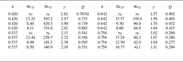
The computed parameters corresponding to the cases shown in figure 7 are summarised in table 1. The circulation increases slightly with decreasing Weber number for a fixed value of
 $b$
, but it decreases significantly as
 $b$
increases and the size of the hollow vortex decreases. The circulation is directly correlated with the scale factor
 $Q$
.
Computed parameters for the cases shown in figure 7.

3.3. Hollow vortex in a corner
Figure 8 illustrates the equilibrium configurations of hollow vortices in a corner with a half-angle
 $ \alpha = \pi /4$
for several values of the parameter
 $ b$
. Although the cavitation number is not defined for
 $ \alpha \neq \pi /2$
, the parameter
 $ b$
still governs the overall size of the vortex in the same manner as in the flat-wall case (
 $ \alpha = \pi /2$
). As
 $ b$
increases, the vortex becomes smaller and the free surface flattens: the amplitude of the shorter waves decreases, and only waves of with larger wavelength are observed as the Weber number decreases. This behaviour indicates a stronger influence of inertial forces relative to surface tension. The olive-coloured curve corresponds to the limiting configuration with self-intersection for which a converged solution can still be obtained.
Free-surface configurations in the corner
 $2\alpha =\pi /2$
for different Weber numbers and for several values of the parameter
 $ b$
: (a) 0.33, (b) 0.42, (c) 0.64. The initial scale factor is
 $ Q_{\textit{in}} = Q^*$
(i.e.
 $c_{\textit{in}}=1$
).

The same as in figure 8 for the corner angle
 $2\alpha =3\pi /2$
and
 $ b$
values (a) 0.33, (b) 0.42, (c) 0.64.

The overall behaviour of the free-surface configurations in figure 9 for the corner with
 $ 2\alpha = 3\pi /2$
is similar to that observed in the previous cases, except for the configuration shown in figure 9(a). The overall size of the vortex increases, relative to the unit distance from the corner to the centroid, as the Weber number decreases.
4. Conclusions
A wave quantisation phenomenon induced by surface tension has been identified on the free surface of a steady hollow vortex in an irrotational flow confined within a corner geometry. By applying the integral hodograph method, we derived analytical expressions for the complex velocity, the complex potential, and the conformal mapping in the parameter plane. This approach reduces the original boundary-value problem to a singular integral equation for the velocity magnitude along the free surface, once the dynamic boundary condition is imposed.
The formulation involves a free parameter
 $b \in (0, 1)$
, which controls the size of the hollow vortex. As
 $b \to 1$
, the vortex size diminishes, and the solution approaches that of a point vortex. Conversely, as
 $b \to 0$
, the free surface extends towards the stagnation point, which location tends to infinity if the centroid of the vortex cavity is chosen as the characteristic length.
Remarkably, the solution is not unique. For the given values of
 $ D$
,
 $ \alpha$
,
 $ \varGamma$
and
 $ \textit{We}$
, multiple wave modes may exist on the vortex cavity. Conversely, the same wave mode can persist over a range of Weber numbers. Within a specific wave form, variations in the Weber number have only a minor effect on the overall shape of the free surface. The maximum curvature of the free surface consistently occurs near the stagnation points. Neither surface tension nor the quantisation condition significantly affects the location of these high-curvature regions, which act as anchoring points for the wave patterns.
In the limiting case
 $\textit{We} \to \infty$
, the velocity magnitude along the free surface becomes constant, simplifying the problem and allowing an analytical solution in terms of elementary functions. Comparisons with the solution of Christopher & Llewellyn Smith (Reference Christopher and Llewellyn Smith2021) (CLS2021), which was obtained using the Schottky–Klein prime function, suggest that these solutions are equivalent, despite the differing mathematical formulations.
Similar quantised wave patterns can be obtained for other corner angles
 $0\lt 2\alpha \lt 2\pi$
. The results are shown for the
 $2\alpha =\pi /2$
and
 $3\pi /2$
. The stability of hollow vortices with surface tension remains an open question and requires further investigation. However, as pointed out by CLS2021 for the case without surface tension, we may expect the following trend: the family of vortex solutions is likely stable for
 $2\alpha \lt \pi$
, neutrally stable for
 $2\alpha = \pi$
, and unstable for
 $2\alpha \gt \pi$
. Confirming this behaviour in the presence of surface tension would provide valuable insight into the dynamical properties of quantised hollow vortices.
In this work, we considered only half of the flow region, which restricts the study to symmetric solutions only, following CLS2021 and Crowdy, Llewellyn Smith & Freilich (Reference Crowdy, Llewellyn Smith and Freilich2012). It should be noted that the CLS2021 approach, based on the Schottky–Klein prime functions (Crowdy Reference Crowdy2020), encompasses the entire flow region and is potentially applicable to the identification of asymmetric solutions as well. Whether an asymmetric steady configuration of the hollow vortex can exist remains an open question.
Acknowledgements
Y.A.S. would like to thank the Isaac Newton Institute for Mathematical Sciences, Cambridge, for financial support and hospitality during the programme ‘The mathematics of multiphase flows with applications’, when work on this paper was undertaken. This work was supported by EPSRC grant EP/V521929/1.
Funding
This work is supported by the National Natural Science Foundation of China (nos W2541018, 52521009, 52192693, 52192690, 52350410468, W2433140), for which the authors are most grateful.
Declaration of interests
The authors report no conflict of interest.